Automatic acoustic detection of birds through deep learning: the first Bird Audio Detection challenge

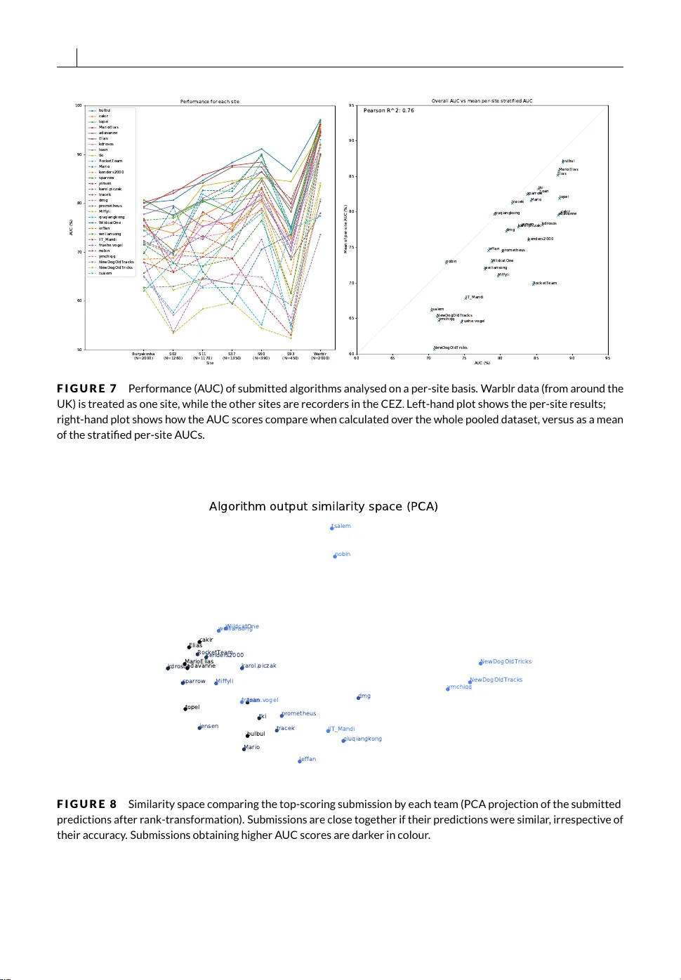
O R I G I N A L A R T I C L E Automatic acoustic detection of birds through deep learning: the fi rst Bird Audio Detection challenge Dan Stowell 1 | Mik e Wood 2 | Hanna P amuła 3 | Y annis Stylianou 4 | Hervé Glotin 5 1 Machine Listening Lab, Centre for Digital Music, Queen Mary University of London. 2 Ecosystems and Environment Research Centre, School of Environment and Life Sciences, University of Salford. 3 Department of Mechanics and Vibroacoustics, AGH University of Science and T echnology , 30-059 Kraków 4 Computer Science Department, University of Crete. 5 LSIS UMR CNRS, University of T oulon, Inst. Univ . de France Correspondence Dan Stowell, Machine Listening Lab, Centre for Digital Music, Queen Mary University of London, London, UK. Email: dan.stowell@qmul.ac.uk Funding information EPSRC fellowship EP /L020505/1; NER C grant NE/L000520/1; ERASMUS+; AGH Research Grant No 15.11.130.642 Assessing the presence and abundance of birds is impor- tant for monitoring speci fi c species as well as over all ecosys- tem health. Many birds are most readily detected by their sounds, and thus passive acoustic monitoring is highly appro- priate. Y et acoustic monitoring is often held back by practi- cal limitations such as the need for manual con fi guration, re- liance on example sound libraries, low accuracy , low robust- ness, and limited ability to generalise to novel acoustic con- ditions. Here we report outcomes from a collaborative data challenge showing that with modern machine learning in- cluding deep learning, general-purpose acoustic bird detec- tion can achieve very high retrieval rates in remote monitor- ing data — with no manual recalibration, and no pre-training of the detector for the target species or the acoustic con- ditions in the target environment. Multiple methods were able to attain performance of around 88% A UC (area under the ROC curve), much higher performance than previous general-purpose methods. We present new acoustic moni- toring datasets, summarise the machine learning techniques proposed by challenge teams, conduct detailed performance evaluation, and discuss how such approaches to detection can be integrated into remote monitoring projects. Ke ywords: bird, sound, machine learning, deep learning, passive acoustic monitoring 1 2 S TO W EL L E T A L ., A U T O M AT I C A C O U S T I C D E T E C T I O N O F B I R D S 1 | I N T R O D U C T I O N Worldwide, bird populations hav e exhibited steep declines since the 1970s, largely due to changes in land management RSPB ( 2013 ); North American Bird Conservation Initiative ( 2016 ). Bird populations are also expected to change in number and distribution as the impacts of climate change play out in coming years ( Johnston et al. , 2013 ). It is thus crucial to monitor avian populations, for the purposes of conservation, scienti fi c research and ecosystem management. This has traditionally been performed via manual surveying, often including the use of volunteers to help address the challenges of scale ( Johnston et al. , 2014 ; Kamp et al. , 2016 ). However , manual observation remains limited, especially in areas that are physically challenging to access, or night-time behaviour . Many bird species are readily detectable by their sounds, often more so than by vision, and so with modern remote monitoring stations able to capture continuous audio recordings the prospect opens up of massive-scale spatio-temporal monitoring of birds ( Aide et al. , 2013 ; Furnas and Callas , 2015 ; Hill et al. , 2017 ; Matsubayashi et al. , 2017 ; Frommolt , 2017 ; Knight et al. , 2017 ). The fi rst wav e of such technology performs automatic recording but not automatic detection, relying on manual after-the-fact study of sound recordings ( Furnas and Callas , 2015 ; Frommolt , 2017 ). Later projects have employed some form of automatic detection, which might be based on low-complexity signal processing such as energy thresholds or template matching ( T owsey et al. , 2012 ; Colonna et al. , 2015 ), or on machine learning algorithms ( Aide et al. , 2013 ). However , when used for fi eld deployments, practitioners face a common hurdle. With the current state of the art, all methods require manual tuning of algorithm parameters, customisation of template libraries and/ or post-processing of results, often necessitating some degree of expertise in the underlying method. The methods are not inherently able to generalise to new conditions—whether those conditions be differing species balances, noise conditions, or recording equipment. Many methods also exhibit only moderate accuracy , which is tolerable in small surveys but leads to unfeasible amounts of false-negatives and -positives in large surveys ( Marques et al. , 2012 ). A further common limitation is the lack of robustness in particular to weather noise: sounds due to rain and wind are commonly observed to dramatically affect detector performance, and as a result surveys may need to treat weather-affected recording periods as missing data. Recent decades have witnessed e xtremely strong growth in the abilities of machine learning. The advances are due to increased dataset sizes and computational power but also due to deep learning methods that can learn to make predictions in e xtremely nonlinear problem settings, such as speech recognition or visual object recognition ( LeCun et al. , 2015 ). These methods have indeed been applied to bioacoustic audio tasks ( Goëau et al. , 2016 ; Salamon and Bello , 2017 ; Knight et al. , 2017 ), and it is clear that their use could enable many organisations to work more cheaply and ef fi ciently ( Joppa , 2017 ). However , even with the strong performance of modern machine learning there remain important questions about generalisability ( Knight et al. , 2017 ). Machine learning work fl ows use a “training set” of data from which the algorithm “learns” , optionally a “validation set” used to determine when the learning has achieved a satisfactory level, and then a “testing set” which is used for the actual evaluation, to estimate the algorithm ’s typical performance on unseen data. Such evaluation is typically performed in matched conditions , meaning the training and testing sets are drawn from the same pool of data, and thus general properties of the datasets—such as the number of positive versus negative cases—are expected to be similar . This enables users to test that the algorithm can generalise to new items drawn from the same distribution. However , in practical deployments of machine learning the new items are rarely drawn from the same distribution: conditions drift, or the tool is applied to new data for which no training data are available ( Sugiyama and Kawanabe , 2012 ; Knight et al. , 2017 ). This is one reason that accuracy results obtained in research papers might not translate to the fi eld. In order to address such problems, we designed a public evaluation campaign focused on a highly-general version of the bird detection task, intended speci fi cally to encour age detection methods which are able to generalise well: agnostic S TO W E L L E T A L ., A U TO M AT I C A C O U S T I C D E T E C T I O N O F B I R D S 3 to species, and able to work in unseen acoustic environments. In this work we present the new acoustic datasets we collated and annotated for the purpose, the design of the challenge, and its outcomes, with new deep learning methods able to achieve strong results despite the dif fi cult task. We analyse the submitted system outputs for their detection ability as well as their robust calibration, we perform a detailed error analysis to inspect the sound types that remain dif fi cult for machine learning detectors, and apply the leading system to a separate held-out dataset of night fl ight calls. We conclude by discussing the new state of the art represented by the deep learning methods that ex celled in our challenge, the quality of their outputs and the feasibility of deployment in remote monitoring projects. 2 | M A T E R I A L S A N D M E T H O D S T o conduct the evaluation campaign we designed a detection task to be solved—speci fi c but illustrative of general- purpose detection issues—gathered multiple datasets and annotated them, and then led a public campaign evaluating the results submitted by various teams. After the campaign, we performed detailed analysis of the system outputs, inspecting questions of accuracy , generality and calibration. Our aim to facilitate general-purpose robust bird detection, agnostic to any speci fi c application, was key to how we designed the challenge speci fi cation. The task of ‘ detecting’ birds in audio can be operationalised in multiple ways: for example, a system that emits a trigger signal in continuous time representing the onset of each bird call, a system that identi fi es regions of pix els in a spectrogram representation (time-frequency ‘box es’), or a system that estimates the number of calling individuals in a given time region ( Benetos et al. , 2018 ). F or any given application, the choice of approach will depend on the requirements for downstream processing. We selected an option which we consider gave wide relevance, while also being a task that could be solved by diverse methods, from simple energy detection, through to template matching or machine learning. This was that audio should be divided into ten-second clips, and the task speci fi cation would be to label each clip with a binary label indicating the presence or absence of birds. This approach quantises time such that any positive detection should be time-localisable within ± 10 seconds, which is suf fi cient for most purposes. It also restricts such that there is no indication of the absolute number of bird calls detected within a positively-labelled clip; however this is hard to ground-truth accurately . Also via statistical ecology methods relative abundances may still be inferred from the distribution of positive detections ( Marques et al. , 2012 ). A concrete advantage of this approach was that it was much quicker to gather manual data annotations than would be the case for more complex labelling. 2.1 | Datasets We gathered and annotated datasets from multiple sources. The purpose of this was twofold: fi rstly to provide better evaluation of the generality of algorithms, and secondly to provide challenge participants with development data (e.g. to perform trial runs, or to train machine learning algorithms) in addition to testing data. We used audio data from remote monitoring projects and also from crowdsourced audio recordings. These two dataset types differ from each other in many ways, for example: remote monitoring audio was passively gathered, while crowdsourced audio recordings were actively captured; the ratio of positive and negative items was different; remote monitoring used fi xed and known recording equipment, while crowdsourcing used uncontrolled equipment. These differences were deliberately introduced for their use in ensuring that the challenge would be a strong test of generalisation. 4 S TO W E L L E T A L ., A U TO M AT I C A C O U S T I C D E T E C T I O N O F B I R D S Codename Habitat Radiation Buryako vka (TBC) Low S2 Deciduous forest Medium S11 Meadow area Medium S37 Pine forest High S60 Shrub area Low S93 Mixed forest High T A B L E 1 Recording locations in Chernobyl dataset. Chernobyl dataset: Our primary remote-monitoring dataset was collected in the Chernobyl Ex clusion Zone (CEZ) for a project to investigate the long-term effects of the Chernobyl accident on local ecology ( Wood and Beresford , 2016 ; Gashchak et al. , 2017 ). The project had captured over 10,000 hours of audio since June 2015, across various CEZ environments, using Wildlife Acoustics SM2 units. For the present work we selected six of recording locations representing different environments (T able 1 ), and from those selected a deterministic subsample: continuous 5-minute audio segments at hourly intervals, across multiple days. Annotators manually labelled all time intervals in which birds were heard (using Rav en Pro software), and then we split recordings and metadata automatically into ten-second segments. The number of fi les per location is uneven because of limited annotator time, giving us 6,620 items in total. No weather fi ltering or other rejection of dif fi cult regions was applied. W arblr dataset: Our fi rst crowdsourced dataset came from a UK-wide project W arblr . W arblr is a software app available for Android and Apple smartphones, which offers automatic bird species classi fi cation (using the method of Stowell and Plumbley ( 2014a )) for members of the public via the submission of ten-second audio recordings. We extracted a dataset of 10,000 audio fi les gathered in 2015–2016. The audio fi les were thus actively collected, recorded on diverse mobile phone devices, and likely to contain various human noise such as speech and handling noise. No assumptions can be made that the data were a representative sample of geographic locations, weather conditions, or bird species. Metadata for the fi les indicated that they covered all the UK seasons, many times of day (with a bias towards weekends and mornings) and geographically spread all around the UK, with a bias toward population centres. All recordings were selected that fell within the time window of available data, limited to a maximum of 10,000. No selection or fi ltering of the data were performed beyond the self-selection inherent in crowdsourcing. Although the data included automatic estimates of which bird species were present, these were not precise enough to be converted to ground-truth data for the detection challenge. We thus performed manual annotation, with each item being labelled as positive or negative according to the challenge speci fi cation. Most items were single- annotated, although we were able to obtain double-annotation for a small number of items, which allowed us to estimate inter-rater reliability . Annotation was performed by experienced listeners using headphone listening and a simple web interface. free fi eld1010 dataset: Our second crowdsourced dataset was an existing public dataset called free fi eld1010 Stowell and Plumbley ( 2014b ). This consists of 7690 audio clips selected from the Freesound online audio archive. T o create this dataset the audio clips had been selected such that they were labelled with the ‘ fi eld-recording’ tag in the database, and trimmed to ten seconds duration. The data were of different origin than Warblr: they covered a global geographic range, and the recording devices used were almost never documented, but likely to include hand-held audio recorders as used by pro-amateur sound recordists, as well as some mobile phones and some higher-end S TO W E L L E T A L ., A U TO M AT I C A C O U S T I C D E T E C T I O N O F B I R D S 5 recording devices. The Freesound database is crowdsourced and thus largely uncontrolled. These data did not come with labels suitable for our challenge; instead, each item came with a set of freely-chosen tags to indicate the content generally . We investigated the ‘birdsong’ tag, one of the most commonly used (2.6% of items), but found this insuf fi ciently accurate. We therefore had these audio annotated through the same process as the W arblr data. PolandNFC dataset: The last dataset contains recordings from one author’s (HP) project of monitoring autumn noc- turnal bird migration. The recordings were collected every night, from September to November 2016 on the Baltic Sea coast, near Darlowo, Poland. We used Song Meter SM2 units with weather-resistant, directional Night Flight Calls microphones from Wildlife Acoustics Inc., mounted on 3–5 m poles. The amount of collected data (>3200 h of recordings) e xceeded what human expert can annotate manually in reasonable time. Therefore we subjectively chose and manually annotated the subset consisting of 22 half-hour recordings from 15 nights with different weather conditions and background noise including wind, rain, sea noise, insect calls, human voice and deer calls. No other selection criterion or weather fi ltering was applied. Manual annotation was performed by visual inspection of a spectrogram and listening to the audio fi les. Only the passerine migrant calls were annotated (voices in 5–10 kHz range ), so it may happen that some low pitched bird species (e.g. resident owl calls) obtained no-bird label. However , such calls were extremely rare in described dataset, so this did not bias results signi fi cantly . The selected recordings were then split into 1 s clips. The chosen clip length, different from other datasets, was chosen due to nocturnal bird calls typical duration (10–300 ms). More details about the dataset structure (and analysis of the effect of audio clip duration) may be found in Pamuła et al. ( 2017 ). All sound fi les used in the public challenge were normalised in amplitude and sav ed as 16-bit single-channel PCM at 44.1 kHz sampling rate, 1 and are available under open licences (see Data Accessibility statement). Our data annotation process was designed after early community discussions about how the challenge should be conducted. We resolved that the annotations should re fl ect plausible annotation conditions as encountered in applications. In particular , they should be well-annotated, yet any mislabellings discovered in the groundtruth data as the challenge progressed should not be eliminated, since training data in practice do contain some errors and are not subject to the same scrutiny as in a data challenge. A good detection algorithm must be able to cope with a small level of imprecision in the annotation data. However , it was possible at the end of the challenge to perform further analysis and inspect the degree of machine errors and human errors. T o make good use of annotator time we used mismatch between automatically inferred decisions and manual annotations to search for mislabelled items in the dataset. For this we used the mean decision from the strongest three submissions to the challenge. All items in the testing set with a negative groundtruth label but a mean decision greater than 0.2, and all items with a positive groundtruth label but a mean decision less than 0.3, were examined and relabeled if needed. One might expect the threshold for re-validation to be 0.5: the asymmetry is because systems generally e xhibited a bias towards low con fi dence, as will be seen later (Section 3.1 ). This re-validation process re fi ned the testing set, but also allowed us to calculate a value for the inter-rater agreement for manual annotation, which we will express as an AUC for comparison against the results of automatic detection. Note that the re-validation process requires the time of e xpert listeners, and so it was not feasible to perform mass crowdsourcing on the whole collection. 1 Normalisation via the sox tool using gain -n -2 . 6 S TO W E L L E T A L ., A U TO M AT I C A C O U S T I C D E T E C T I O N O F B I R D S 2.2 | Baseline classi fi ers T o establish baseline performance against which to compare new methods, we used two existing machine-learning based classi fi cation algorithms. The fi rst (code-named smacpy ) was the same baseline classi fi er as used in a 2013 challenge on “detection and classi fi cation of acoustic scenes and events” (“DCASE”) ( Stowell et al. , 2015 ). This baseline classi fi er represents a well-studied method used in many audio classi fi cation tasks: audio is converted to a representation called mel frequency cepstral coef fi cients (MFCCs), and the distributions of MFCCs are then modelled using Gaussian mixture models (GMMs). Such an approach is simple, ef fi cient and adaptable to many sound recognition tasks. It has been superseded for accuracy in general-purpose sound recognition by more advanced methods ( Stowell et al. , 2015 ). We selected it to provide a common low-comple xity baseline, and also because its simplicity meant it might successfully avoid over fi tting to the training data, i.e. avoid becoming overspecialised, given that the training and test data would have different characteristics. The second baseline (code-named sk fl ) was a recent and more powerful classi fi er introduced for bird species recog- nition ( Stowell and Plumbley , 2014a ). This was the strongest audio-only bird species classi fi er in a 2014 international evaluation campaign. Relative to smacpy it innovated in both the feature representation and the classi fi cation algorithm. The feature representation was an automatically-learnt data transformation: two layers of “unsupervised feature learning” applied to Mel spectrogram input. For classi fi cation the method used a random forest, an ensemble learning method based on decision trees that has emerged as powerful and robust for many tasks in machine learning ( Breiman , 2001 ). Both of these components are known to work well with dif fi cult classi fi cation scenarios, such as multi-modal classes, unbalanced datasets, and outliers. We thus selected this second baseline as a representative of modern and fl exible machine learning, designed for bird sounds. In principle it could be more vulnerable to over fi tting than the fi rst baseline. However , because of the inherent dif fi culty of the task, we expected sk fl to perform more strongly than smacpy , and to provide a high performing baseline. Python code for each of the baseline classi fi ers has previously been published ( Stowell and Plumbley , 2014a ; Stowell et al. , 2015 ). Initial results using the baseline classi fi ers were published online as a guide to the challenge participants. 2 2.3 | The public challenge Conduct of the public challenge followed the design of previous successful contests on related topics ( Stowell et al. , 2015 ; Goëau et al. , 2016 ). Having already determined the need for the challenge from remote monitoring liter ature and practitioners ( Stowell et al. , 2016 ), we announced intentions and led community discussion on the task design via a dedicated mailing list. We collated our audio datasets into three portions: development data to be publicly shared (7,690 items of free fi eld1010 plus 8,000 items from W arblr), testing data whose true labels were to be kept private (10,000 items from Chernobyl plus 2,000 items from Warblr), and a separate set not used for the challenge itself but for further study of algorithm generalisation (PolandNFC). Providing two distinct development data sets allowed participants to test generalisation from one to the other , as part of their own algorithm development process, while k eeping some datasets fully private allowed us to evaluate generalisation without concern that algorithms might have been con fi gured to the speci fi cs of a given dataset. The public development datasets were distributed in September 2016, both audio and groundtruth annotations. T eams could then begin to develop methods and train their systems. In December 2016 we released the testing data 2 http://machine- listening.eecs.qmul.ac.uk/ 2016 / 10 /bird- audio- detection- baseline- generalisation/ S TO W E L L E T A L ., A U TO M AT I C A C O U S T I C D E T E C T I O N O F B I R D S 7 (audio only), with a one month deadline for the submission of inferred detection labels. The short time horizon of one month was intended to minimise the opportunity for overly adapting the methods to the characteristics of the testing data. During this period, teams could make multiple submissions, but limited to a maximum of one per day . "Preview" results, calculated from 15% of the testing data, were provided in an interactive online plot, in order to give appro ximate feedback on performance (Figure 2 ). Participants were allowed to run their software on their own machines and then to submit merely the outputs (as opposed to the software code), which our online system would then score without revealing the groundtruth labels for the testing data. Given that this open approach has potential vulnerabilities—such as recruiting manual labellers rather than developing automatic methods—we required the highest-scoring teams to send in their code which we inspected and re-ran on our own systems, to ensure a fair outcome. Aside from intrinsic motivation, incentives for participants were cash prizes: one for the strongest scoring system , and one judges’ award decided according to the use of interesting or novel methodology . This was done to stimulate conceptual development in the fi eld, as opposed to the mere application of off-the-shelf deep learning. Participants were further required to submit technical notes describing their method, and later were invited to submit peer-reviewed conference papers to a special session at the European Signal Processing Conference (EUSIPCO) 2017. Of these, 8 challenge-related papers were accepted and presented. The challenge organisation was thus designed to achieve the following: public benchmarking of methods against a common task and data, speci fi cally tailored to fully-automatic con fi guration-free bird detection in unseen conditions; public documentation of the methods used to achieve leading results; and greater attention from machine learning researchers on data analysis tasks in environmental sound monitoring. 2.4 | Evaluation Our goal was to evaluate algorithms for their ability to perform general-purpose bird detection, within the selected format of binary decisions for ten-second audio clips. A strong algorithm is one that can reliably separate the two classes “bird(s) present” and “no bird present” . However , since our evaluation was general and not targeted at a speci fi c application, we wished to generalise over the possible tradeoffs of precision versus recall (the relative cost of false- positive detections versus false-negative detections). This strongly motivated our design such that participants should return probabilistic or graded outputs—a real-valued prediction for each audio clip rather than simply a 1 or 0—and our evaluation would use the well-studied area under the ROC curve (AUC) as the primary quality metric. The AUC measure has numerous qualities that mak e it well-suited to evaluation such classi fi cation tasks: it generalises over all the possible thresholds that one might apply to real-valued detector outputs; unlike raw accuracy , it is not affected by “unbalanced” datasets having an uneven mixture of positive and negative items; chance performance for AUC is always 50% irrespective of dataset; and it has a probabilistic interpretation, as the probability that a given algorithm will rank a randomly-selected positive instance more highly than a randomly-selected negative instance ( Fawcett , 2006 ). The ranking interpretation just mentioned highlights another aspect of the AUC statistic: it treats detector outputs essentially as rank ed values and is thus invariant to any monotonic mapping of the outputs, in particular to whether the outputs are well-calibrated probabilities or not. Well-calibrated, in this context, implies that when a detector outputs "0.75" for an item, this matches the empirical probability that in three out of four such cases the item is indeed a positive instance ( Niculescu-Mizil and Caruana , 2005 ). Thus AUC does not evaluate calibration. But the need for calibration depends on the application: if a detector is being used to select a subset of strong detections, or to rank items for further manual inspection, there may be no need for calibration. However if the detections are to be used in some probabilistic model e.g. for modelling a population 8 S TO W E L L E T A L ., A U TO M AT I C A C O U S T I C D E T E C T I O N O F B I R D S distribution, it is desirable for a detector to output well-calibrated probabilities. If a detector performs well in the sense evaluated by A UC, then its outputs can be mapped to probabilities by a post-processing step ( Niculescu-Mizil and Caruana , 2005 ). Hence, we used AUC as our primary measure of quality , and separately we analysed the calibration of the submitted algorithms using the method of calibration plots , which are histogram plots comparing outputs against empirical probabilities ( Niculescu-Mizil and Caruana , 2005 ). 2.5 | F urther analysis via PolandNFC dataset After the challenge concluded we took the highest-scoring algorithm and applied it to the PolandNFC dataset, an unseen and dif fi cult dataset containing night fl ight calls, often brief and distant. We used this in two ways: (a) trained on a held-out portion (72.7 %) of the PolandNFC data and tested on the remaining 27.3%; (b) tr ained using the main challenge development data and again tested on the 27.3% of the PolandNFC data. This allowed us to evaluate further the generalisation capability learnt by the network. For variant (a), the training dataset consisted of sixteen 30 min recordings collected over 11 nights (split into 28,784 1 s clips), and the testing dataset had six recordings from 4 nights (split into 10,793 1 s clips). T raining and testing recording dates were disjoint sets. The testing set was held the same across variant (a) and (b) to ensure comparability of results. Important to note is the speci fi c structure of the PolandNFC dataset—it contains mostly negatively annotated examples (only 3.2 % for testing and 1.6 % for training set were positive ). 3 | R E S U LT S In re-validating the testing set we examined those items with the strongest mismatch between manual and automatic detection, to determine which was in error: 500 presumed negative and 1243 presumed positive items. This showed inter-rater disagreement in 16.6% of such cases—predominantly , the most ambiguous cases with barely-audible bird sounds with amplitude close to the noise threshold. Note that this percentage is not representative of disagreement across the whole dataset, but only on the ‘contro versial’ cases. We also observed that a strong mismatch according to the automatic detectors did not necessarily imply human mislabelling: some perceptually obvious data items could be consistently misjudged by algorithms. We will discuss algorithm errors further below. Through re-validation the inter-rater reliability , measured via the AUC, was measured as 96.7%. This value provides an approximate upper limit for machine performance since it re fl ects the extent of ambiguity in the data according to human listeners’ perception. The two baseline classi fi ers gave relatively good performance on the development data, the strongest at over 85% AUC in matched conditions, but generalised poorly . The simpler GMM-based baseline classi fi er showed consistently lower results than the more advanced classi fi er , as expected. It also showed strong resistance to over fi tting in the sense that its performance on its training set was a very good predictor of its performance on a matched-conditions testing set. However , this was not suf fi cient to allow it to generalise to mismatched conditions, in which its performance degraded dramatically (Figure 1 ). The more advanced baseline classi fi er also degraded when tested in mismatched conditions, though to a lesser extent, attaining 79% AUC. 3.1 | Challenge outcomes Thirty different teams submitted results to the challenge, from various countries and research disciplines, with many submitting multiple times during the one-month challenge period (Figure 2 ). Around half of the teams also submitted S TO W E L L E T A L ., A U TO M AT I C A C O U S T I C D E T E C T I O N O F B I R D S 9 F I G U R E 1 T ests using baseline classi fi ers on the two development datasets. The middle column shows testing results under matched conditions, as commonly reported in machine learning; the rightmost column shows testing results under mismatched conditions, i.e. training with one dataset and testing with the other . system descriptions, of which the majority were based on deep learning methods, often convolutional neural networks (CNNs) (Figure 3 ). T o preprocess the audio for use in deep learning, most teams used a spectrogram representation, often a "mel spectrogram " , which is a spectrogram with its frequency axis warped to an approximation of human nonlinear frequency-band sensitivity . Many teams also used data augmentation, meaning that they arti fi cially increased the amount of training data by copying and modifying data items in small ways, such as adding noise or shifting the audio in time. These strategies are in line with other work using machine learning for bird sound ( Goëau et al. , 2016 ; Salamon and Bello , 2017 ). Most teams were able to achieve over 80% A UC, but none over 90%: the strongest score was 88.7% AUC, attained by team ‘bulbul’ (Thomas Grill) on the fi nal day of challenge submission (Figure 4 ). The team has given further details of their approach in a short conference publication ( Grill and Schlüter , 2017 ) and with open-source code available online. 3 Inspecting the highest-scoring entries, and estimating their variation through bootstrap sampling, we found that four teams’ results were within the con fi dence interval of the highest score (Figure 5 ). AUC scores are summary statistics of ROC plots. Inspecting the detail of the ROC plots for these four highest- scoring systems and for the lowest-scoring system (Figure 6 ), we fi nd some tendency for the curves to be biased towards an asymmetry (close to the left-hand edge of the plot but not the upper edge). This implies a spread of ‘ dif fi culty’ for the test items: there were some positive items that were easy to detect without incurring extr a false-positives as a side-effect, while many remained dif fi cult to detect. The most balanced of the ROC plots inspected was that of ‘cakir’ , implying that this system had a more balanced distribution of its discriminative power across the easy and dif fi cult cases. Since the testing data consisted of items from multiple ‘sites’ —i.e. known sites in the Chernobyl Exclusion Zone, plus the W arblr (UK) data considered as a separate single site—we were able to calculate the AUC scores on a per-site basis (Figure 7 , left). These showed a strong site-dependency of algorithm performance. Whereas Warblr data could be detected with an AUC of over 95%, Chernobyl sites showed varying dif fi culty for the detectors over all, some as low as 80% even for the leading algorithms. However , the overall A UC was very highly predictive of the aver age of the per-site AUCs (Pearson R 2 = 0 . 76 ; Figure 7 , right). Note that the two AUC calculations are not independent and so some correlation is e xpected. The observed correlation validates that the over all AUC is usable as a summary of the 3 https://jobim.ofai.at/gitlab/gr/bird_audio_detection_challenge_ 2017 /tree/master 10 S TO W E L L E T A L ., A U TO M AT I C A C O U S T I C D E T E C T I O N O F B I R D S 4 5 6 7 8 9 10 11 12 13 14 15 16 17 18 19 20 21 22 23 24 25 26 27 28 29 30 31 Day of challenge 40 50 60 70 80 90 100 AUC score (%) Preview scores (all) F I G U R E 2 Timeline of preview scores attained by every submission for each team. Error bars are estimated by bootstrap sampling. per-site performance. The ‘bulbul’ system remained the strongest performer even under the per-site analysis. The rank ordering of systems was not highly preserved: for example the second-placed ‘ cakir’ system would hav e been rank ed tenth if using the aver age per-site AUC. Applying PCA to the system outputs, we recovered an abstract ‘similarity space’ of systems, which showed that some of the lowest-scoring systems formed two outlier clumps in terms of their predictions, while the stronger systems formed something of a continuum (Figure 8 ). The very strongest scoring systems did not cluster tightly together , indicating that there remains some diversity in the strategies implicit in these high-performing detectors. We measured calibration curves separately for the Warblr and Chernobyl testing data (Figure 9 ). Calibration was generally better for W arblr , as one might expect given the availability of Warblr training data. Notably , the highest- scoring submission ‘bulbul’ had by far the worst calibr ation on the Chernobyl data: around 80% of cases it assigned a prediction value of 0.25 were indeed positive (versus around 30% on the Warblr data). The second-highest-scoring submission ‘cakir’ e xhibited quite different behaviour , remaining relatively well calibrated even when assessing the unseen Chernobyl data. 3.2 | Error analysis We inspected the 500 data items for which the predictions of the strongest systems exhibited mismatch with the re-validated ground truth, to characterise typical errors made by ev en the strongest machine learning systems in bird audio detection (T able 2 ). Such inspection is heuristic, relying on perceptual judgment to estimate the causes of errors; however repeated tendencies give us indications about the performance of the current state of the art. F or false negatives, by far the most common observation was that positive items contained very faint bird sound (e.g. distant), often needing multiple listens to be sure it was present. These faint sounds had low SNR and were often S TO W E L L E T A L ., A U TO M AT I C A C O U S T I C D E T E C T I O N O F B I R D S 11 F I G U R E 3 Overview of the methods used by the submitted systems, and their scores. 12 S TO W E L L E T A L ., A U TO M AT I C A C O U S T I C D E T E C T I O N O F B I R D S 5 7 12 13 19 20 21 22 23 26 28 29 31 Day of challenge 70 75 80 85 90 95 AUC score (%) Elias IIT_Mandi Mario MarioElias Miffyli NewDogOldTracks NewDogOldTricks RocketTeam WildcatOne adavanne bulbul cakir dmg fruehe.vogel jensen karol.piczak kdrosos kenders2000 leffan nobin prometheus qiuqiangkong sparrow tki toan topel tracek tsalem weiliansong ymchiqq Final scores (each team's top submission) F I G U R E 4 Final scores attained by the highest-performing submission for each team. Error bars are estimated by bootstrap sampling. also quite reverberated. Low SNR was also a factor in the third most common presumed cause, noise masking. This category included general broadband ‘pink’ noise sources including wind and rivers. There were other more speci fi c categories of sound that appeared to act as masker or distractor causing systems to overlook the bird sound: insect noise was common in the CEZ data, while human sounds such as speech, whistling, or TV s were present in the W arblr data. The second most common presumed cause of false negatives was howev er the presence of extremely short calls: often a single “chink” sound, which might perhaps be overlook ed or confused with rain-drop sounds. Some sounds were presumed to be missed because they were unusual for the dataset (e.g. goose honking), although this was not seen as a major factor . False positives occurred at a much lower rate in the top 500 most mismatched items. They appeared to be caused in roughly equal proportion by insects, human sounds, and rain sounds (individual drops or diffuse rainfall). 3.3 | F urther analysis via PolandNFC dataset results We then applied the highest-scoring method (‘bulbul’) to the separate and unseen acoustic monitoring dataset Poland- NFC. The bulbul algorithm performed its inference in two stages: the fi rst stage applied the pre-trained neural network to make initial predictions; the second stage allowed the neural network to adapt to the observed data conditions, by feeding back the most con fi dent predictions as new training data ( Grill and Schlüter , 2017 ). We evaluated the outputs from each stage (T able 3 ). AUC results were of high quality and were most strongly affected by the choice of training data, the matched-conditions training yielding much more accurate predictions. The second stage adaptation offered some improvement in the case where the training set came from mismatched conditions. However in matched-conditions training the second stage actually incurred a slight reduction in performance. Calibration plots for this test show that the detector was also better calibrated when trained in matched conditions, and that the second stage re-training did not have a strong effect on calibration (Figure 10 ). S TO W E L L E T A L ., A U TO M AT I C A C O U S T I C D E T E C T I O N O F B I R D S 13 5 9 11 12 14 19 21 22 23 24 29 30 31 Day of challenge 87.0 87.5 88.0 88.5 89.0 89.5 90.0 AUC score (%) Final scores (top 20 submissions only) Elias MarioElias adavanne bulbul cakir topel F I G U R E 5 Final scores attained by the 20 highest-scoring submissions. Error bars are estimated by bootstrap sampling. 0.0 0.2 0.4 0.6 0.8 1.0 False Positive Rate 0.0 0.2 0.4 0.6 0.8 1.0 True Positive Rate ROC plots (selected) bulbul cakir topel MarioElias tsalem F I G U R E 6 ROC plots for the systems attaining the four highest and one lowest AUC score. 14 S TO W E L L E T A L ., A U TO M AT I C A C O U S T I C D E T E C T I O N O F B I R D S Buryakovka (N=2000) S02 (N=1260) S11 (N=1170) S37 (N=1350) S60 (N=390) S93 (N=450) Warblr (N=2000) Site 50 60 70 80 90 100 AUC (%) Performance for each site bulbul cakir topel MarioElias adavanne Elias kdrosos toan tki RocketTeam Mario kenders2000 sparrow jensen karol.piczak tracek dmg prometheus Miffyli qiuqiangkong WildcatOne leffan weiliansong IIT_Mandi fruehe.vogel nobin ymchiqq NewDogOldTracks NewDogOldTricks tsalem 60 65 70 75 80 85 90 95 AUC (%) 60 65 70 75 80 85 90 95 Mean of per-site AUC (%) bulbul cakir topel MarioElias adavanne Elias kdrosos toan tki RocketTeam Mario kenders2000 sparrow jensen karol.piczak tracek dmg prometheus Miffyli qiuqiangkong WildcatOne leffan weiliansong IIT_Mandi fruehe.vogel nobin ymchiqq NewDogOldTracks NewDogOldTricks tsalem Pearson R^2: 0.76 Overall AUC vs mean per-site stratified AUC F I G U R E 7 Performance (A UC) of submitted algorithms analysed on a per-site basis. W arblr data (from around the UK) is treated as one site, while the other sites are recorders in the CEZ. Left-hand plot shows the per-site results; right-hand plot shows how the AUC scores compare when calculated over the whole pooled dataset, versus as a mean of the strati fi ed per-site AUCs. bulbul cakir topel MarioElias adavanne Elias kdrosos toan tki RocketTeam Mario kenders2000 sparrow jensen karol.piczak tracek dmg prometheus Miffyli qiuqiangkong WildcatOne leffan weiliansong IIT_Mandi fruehe.vogel nobin ymchiqq NewDogOldTracks NewDogOldTricks tsalem Algorithm output similarity space (PCA) F I G U R E 8 Similarity space comparing the top-scoring submission by each team (PCA projection of the submitted predictions after rank-tr ansformation). Submissions are close together if their predictions were similar , irrespective of their accuracy . Submissions obtaining higher AUC scores are darker in colour . S TO W E L L E T A L ., A U TO M AT I C A C O U S T I C D E T E C T I O N O F B I R D S 15 0.0 0.2 0.4 0.6 0.8 1.0 Mean predicted value 0.0 0.2 0.4 0.6 0.8 1.0 Fraction of positives Calibration plots (reliability curve), Warblr bulbul cakir topel MarioElias adavanne Elias kdrosos toan tki RocketTeam Mario kenders2000 sparrow jensen karol.piczak tracek dmg prometheus 0.0 0.2 0.4 0.6 0.8 1.0 Mean predicted value 0.0 0.2 0.4 0.6 0.8 1.0 Fraction of positives Calibration plots (reliability curve), Chernobyl bulbul cakir topel MarioElias adavanne Elias kdrosos toan tki RocketTeam Mario kenders2000 sparrow jensen karol.piczak tracek dmg prometheus F I G U R E 9 Calibration plots for the strongest submission by each team, separately for the Warblr test data ( fi rst plot) and Chernobyl test data (second plot). For legibility we have limited this to the submissions attaining at least 80% AUC. A submission whose outputs are well-calibrated probabilities should yield a line close to the identity diagonal. Category False positives False negatives Clear 1 68 Dontknow 7 40 Faint (e.g. v distant) 0 179 Short call 0 69 Noise-masking (inc wind, river) 0 67 Insect 26 52 Human (speech, laughter , tv , imitation) 31 13 Rain (inc drops) 26 5 Unusual bird sound 0 29 Misc distractor 0 11 Misc mammal 2 0 T A B L E 2 Inferred reasons for mistakes made by the strongest-performing systems, annotated for the 500 items for which the systems showed the strongest deviation from groundtruth. Note that the count data sum to more than 500, since multiple reasons could potentially be attributed to each item. “Clear” means the item was perceptually clear and should have been correctly labelled; “Dontknow” means that no obvious reason for a mistake is evident, even if the item is not particularly clear; all other rows are categories of presumed reasons for machine errors. 16 S TO W E L L E T A L ., A U TO M AT I C A C O U S T I C D E T E C T I O N O F B I R D S AUC (%) T raining data First stage Second stage Challenge (mismatched) 83.9 (+/ - 0.4) 87.76 (+/ - 0.07) PolandNFC (matched) 94.95 (+/- 0.01) 93.78 (+/ - 0.01) T A B L E 3 Performance obtained when applying the highest-scoring challenge system to remote monitoring audio data from Poland, av erage of results from two runs of the system. 0.0 0.2 0.4 0.6 0.8 1.0 Mean predicted value 0.0 0.2 0.4 0.6 0.8 1.0 Fraction of positives Calibration plots (reliability curve) BAD_PL_testing_labels_first_stage first stage second stage 0.0 0.2 0.4 0.6 0.8 1.0 Mean predicted value 0.0 0.2 0.4 0.6 0.8 1.0 Fraction of positives Calibration plots (reliability curve) PL_PL_testing_labels_first_stage first stage second stage F I G U R E 1 0 Calibration plots obtained when applying the highest-scoring challenge system to remote monitoring audio data from Poland (cf . Figure 9 ). First plot: Challenge (mismatched) training; second plot: PolandNFC (matched) training. S TO W E L L E T A L ., A U TO M AT I C A C O U S T I C D E T E C T I O N O F B I R D S 17 4 | D I S C U S S I O N T wo broad observations emerge from this study: 1. Machine learning methods, primarily deep learning, are able to achieve very high recognition rates on remote moni- toring acoustic data, despite weather noise, low SNRs, wide variation in bird call types, and even with mismatched training data. The AUC results presented here are a dramatic advance in the state of the art, and machine learning methods are of practical use in remote monitoring projects. 2. However , there remains a signi fi cant gap between performance in matched conditions and in mismatched conditions. T rue generalisation remains dif fi cult, and further work is needed. Projects are thus recommended to obtain some amount of matched-conditions training data where possible, and to treat automatic detection results with some caution especially with regard to the calibration of the outputs if they are to be treated as probabilities or if a fi xed detection threshold is used. (Post-processing such as Platt scaling can ameliorate calibration issues ( Niculescu- Mizil and Caruana , 2005 ).) If a ranked-results approach is used (e.g. keeping the strongest N detections), which circumvents questions of calibration, then performance can remain strong even in mismatched conditions (Fig 7; T able 3 ). In practical applications there are differing tradeoffs of precision versus recall, of false negatives versus false positives. The AUC statistics summarise over these but tell us that whatev er position on the ROC curve is chosen, the improvement in the state of the art which we report can give a much better tradeoff (Fig 6), which corresponds for example to a much lower amount of manual postprocessing time in fi ltering out false-positive results ( Pamuła et al. , 2017 ). The strongest machine learning methods in this study were convolutional and/or recurrent neural nets (CNNs, RNNs, or CRNNs), as has been observed in other domains ( LeCun et al. , 2015 ). In order to ensure methods could work in conditions different from those in the training data, various participants explored self-adaptation, in which a trained network is fi ne-tuned upon exposure to the new conditions (without needing any additional ground-truth information) ( Grill and Schlüter , 2017 ; Çakır et al. , 2017 ; Adavanne et al. , 2017 ). Participants reported mixed results of this, some observing no bene fi t. We found little bene fi t of self-adaptation for matched conditions; however , in cases where matched-conditions training data is not available, we found that it can reduce the adverse effect of the mismatch (T able 3 ). A further practical question is the feasibility of implementation on low-power devices for long-term deployment in the fi eld. Deep learning experiments often require hardware acceleration, primarily for the training phase. After training, deep learning algorithms can be deployed onto smaller embedded units ( Mac Aodha et al. , 2018 ). However , the self-adaptation methods considered here are essentially additional rounds of training, albeit conducted with unlabelled data, and thus would incur quite some cost for use in the fi eld. A pragmatic version of this would be to perform training or ‘pre-training’ using mismatched data, then collecting a small amount of matched data from the target fi eld conditions to perform self-adaptation, before fi xing the algorithm parameters for use on-device. Our error analysis showed that the most common error for the present generation of algorithms appears to be false-negatives due to the failure to detect faint/ distant bird sound. The next most salient concern is robustness to masking noise (wind, river , insects, speech). There were many entries which were very hard to decide, as a listener: faint, short, and masked sounds together constitute a large portion of items. This perceptual dif fi culty , re fl ected in inter-rater disagreements, reminds us that some cases may be inherently ambiguous and thus may always be dif fi cult for machine recognition. However , there is still a fair proportion (more than 1 in 10 of the top 500 items inspected) for 18 S TO W E L L E T A L ., A U TO M AT I C A C O U S T I C D E T E C T I O N O F B I R D S which the sound recording was judged to be perceptually clear , meaning that the reason for those false negatives is due to a detector failing to model bird sound correctly , providing scope for algorithm improvements. A further speci fi c cause of detector errors stems from the ambiguity between very short ‘chink’ bird calls and sounds such as individual rain drops which hav e similar effects in a spectrogram. A related issue was observed in bats, with the very short calls of species in the Myotis genus being the most dif fi cult to disambiguate according to Walters et al. ( 2012 ). If the observable attributes of multiple sources overlap entirely then it is not possible to distinguish them even in principle. However , at least in our case human listeners can tell the difference, whether from context or from fi ne detail of signals. We thus expect that future work on higher-resolution input features—such as waveform data rather than spectrogram data—will be able to improve on this issue. Hutto and Stutzman ( 2009 ) previously performed an analysis of human sound detection of birds. Their comparison was between humans and “autonomous recording units”: however , note that in the latter case the detection was performed manually by inspecting spectrograms and listening to recordings, contrasted against a human listener in the fi eld. Their results are thus not directly comparable to ours; howev er they too found that distant bird sounds were the predominant cause of missed detections for remote sensing units. Furnas and Callas ( 2015 ) likewise studied in- fi eld versus audio-based detection using manual annotation, with similar results. They noted that detection probability could vary according to situational factors such as elevation and tree canopy cover . Digby et al. ( 2013 ) compared evaluated automated detection in audio against in- fi eld manual detection, for a single species (the little spotted kiwi, Apteryx owenii ), fi nding detection rates of around 40% with a relatively simple detection algorithm; despite this, they concluded that the high ef fi ciency of automatic methods led to a large reduction in person-hours and thus was recommended. They found that wind noise e xerted a larger in fl uence on automatic detection than on manual detection. Over all, our study design via a data challenge has been successful in moving forward the state of the art in acoustic remote monitoring. The design as a binary classi fi cation task, evaluated by A UC, is recommended as a way to generalise over some diversity in requirements among remote monitoring projects, with the calibration analysis as an important addition to AUC evaluation. The use of multiple test sets sourced from different projects is a robust approach for general-purpose evaluation of algorithms, and we further recommend the use of per-site strati fi ed A UC to account for per-site differences. 4 This complements the task-speci fi c evaluation that a well-resourced individual project should undertake (cf . Knight et al. ( 2017 )). Going beyond the “yes/ no ” binary classi fi cation task, in some cases is desirable to identify individual bird calls: the binary classi fi cation paradigm can in fact enable this, through a procedure of “weakly supervised learning” ( Mor fi and Stowell , 2017 ; Mor fi and Stowell , 2018 ; Kong et al. , 2017 ). In future evaluations we recommend the explor ation of such approaches, combining broad-scale detection with the elucidation of fi ner detail. 4 The second edition of the Bird Audio Challenge, launched at time of writing, incorporates these recommendations, using per-site strati fi ed AUC as well as adding further test sets to the challenge. http://dcase.community/challenge 2018 /task- bird- audio- detection S TO W E L L E T A L ., A U TO M AT I C A C O U S T I C D E T E C T I O N O F B I R D S 19 A C K N O W L E D G M E N T S We would like to thank Paul Kendrick for preparation and annotation of Chernobyl data, Luciana Barçada for annotation of Chernobyl data, and Julien Ricard for programming and administering the challenge submission website. We also thank the many challenge participants for their enthusiastic effort. A U T H O R C O N T R I B U T I O N S DS, MW , YS and HG designed the data challenge study and its analysis; DS, MW and HP provided datasets; HG led the creation of the challenge submission website; DS and HP performed tests of machine learning systems; DS, HG and HP analysed the results; DS led the writing of the manuscript, with some sections by HP . All authors contributed critically to the drafts and gave fi nal approval for publication. D A T A A C C E S S I B I L I T Y • De velopment datasets: both audio and annotations are available under CC -BY -4.0 licences. warblrb10kaudio: https://archive.org/details/warblrb 10 k_public ff1010bird audio: https://archive.org/details/ff 1010 bird Annotations: https://doi.org/ 10 . 6084 /m 9 .figshare. 3851466 .v 1 • T esting data (Chernobyl/warblrb10k): audio public, but annotations held back for future challenges. Audio: https://archive.org/details/birdaudiodetectionchallenge_test • P olandNFC data: held back, in preparation for future challenge. • Source code for baseline classi fi ers: GMM ‘smacpy’ classi fi er (MIT licence): https://github.com/danstowell/smacpy . sk fl feature-learning is available as supplementary information in Stowell and Plumbley ( 2014a ) (MIT licence). • Source code for the online submission website (MIT licence): https://github.com/julj/submission • Source code and papers for various of the systems submitted by challenge teams are available via http://c 4 dm. eecs.qmul.ac.uk/events/badchallenge_results/ (various licences). R E F E R E N C E S Adavanne, S., Parascandolo, G., Drossos, K., Virtanen, T . et al. (2017) Convolutional recurrent neural networks for bird audio detection. In Proceedings of EUSIPCO 2017 . Special Session on Bird Audio Signal Processing. Aide, T . M., Corrada-Br avo, C., Campos-Cerqueira, M., Milan, C., Vega, G. and Alvarez, R. (2013) Real-time bioacoustics moni- toring and automated species identi fi cation. PeerJ , 1 , e103. Benetos, E., Stowell, D. and Plumbley , M. D. (2018) Approaches to complex sound scene analysis. In Computational Analysis of Sound Scenes and Events , chap. 8, 215–242. Springer . Breiman, L. (2001) Random forests. Machine Learning , 45 , 5–32. Çakır , E., Par ascandolo, G., Heittola, T ., Huttunen, H. and Virtanen, T . (2017) Convolutional recurrent neural networks for poly- phonic sound event detection. IEEE T r ansactions on Audio, Speech and Language Processing, Special Issue on Sound Scene and Event Analysis . ArXiv preprint Colonna, J. G., Cristo, M., Salvatierra, M. and Nakamura, E. F . (2015) An incremental technique for real-time bioacoustic signal segmentation. Expert Systems with Applications . 20 S TO W E L L E T A L ., A U TO M AT I C A C O U S T I C D E T E C T I O N O F B I R D S Digby , A., T owsey , M., Bell, B. D. and T eal, P . D. (2013) A practical comparison of manual and autonomous methods for acoustic monitoring. Methods in Ecology and Evolution , 4 , 675–683. Fawcett, T . (2006) An introduction to ROC analysis. Pattern Recognition Letters , 27 , 861–874. Frommolt, K. -H. (2017) Information obtained from long-term acoustic recordings: applying bioacoustic techniques for moni- toring wetland birds during breeding season. Journal of Ornithology , 1–10. Furnas, B. J. and Callas, R. L . (2015) Using automated recorders and occupancy models to monitor common forest birds across a large geographic region. The Journal of Wildlife Management , 79 , 325–337. URL: http://dx.doi.org/ 10 . 1002 /jwmg. 821 . Gashchak, S., Gulyaichenk o, Y ., Beresford, N. A. and Wood, M. D. (2017) European bison (bison bonasus) in the chornobyl ex clusion zone (ukraine) and prospects for its revival. Proceedings of the Theriological School , 15 , 58–66. Goëau, H., Glotin, H., V ellinga, W . -P ., Planqué, R. and Joly , A. (2016) LifeCLEF bird identi fi cation task 2016: The arrival of deep learning. In Working Notes of CLEF 2016-Conference and Labs of the Evaluation forum, Évora, Portugal, 5-8 September , 2016. , 440–449. Grill, T . and Schlüter , J. (2017) T wo convolutional neural networks for bird detection in audio signals. In Proceedings of EUSIPCO 2017 . Special Session on Bird Audio Signal Processing. Hill, A. P ., Prince, P ., Covarrubias, E. P ., Doncaster , C. P ., Snaddon, J. L. and Rogers, A. (2017) AudioMoth: Evaluation of a smart open acoustic device for monitoring biodiversity and the environment. Methods in Ecology and Evolution . URL: https:// doi.org/ 10 . 1111 % 2 F 2041 - 210 x. 12955 . Hutto, R. L . and Stutzman, R. J . (2009) Humans versus autonomous recording units: a comparison of point-count results. Jour- nal of Field Ornithology , 80 , 387–398. Johnston, A., Ausden, M., Dodd, A. M., Bradbury , R. B., Chamberlain, D. E., Jiguet, F ., Thomas, C. D., Cook, A. S., Newson, S. E., Ockendon, N. et al. (2013) Observed and predicted effects of climate change on species abundance in protected areas. Nature Climate Change , 3 , 1055–1061. Johnston, A., Newson, S. E., Risely , K., Musgrove, A. J., Massimino, D., Baillie, S. R. and Pearce-Higgins, J. W . (2014) Species traits explain variation in detectability of uk birds. Bird Study , 61 , 340–350. Joppa, L . N. (2017) Comment: The case for technology investments in the environment. Nature . URL: https://www.nature. com/articles/d 41586 - 017 - 08675 - 7 . Kamp, J., Oppel, S., Heldbjerg, H., Nyegaard, T . and Donald, P . F . (2016) Unstructured citizen science data fail to detect long- term population declines of common birds in denmark. Diversity and Distributions . Knight, E., Hannah, K., Fole y , G., Scott, C., Brigham, R. and Bayne, E. (2017) Recommendations for acoustic recognizer per- formance assessment with application to fi ve common automated signal recognition programs. Avian Conservation and Ecology , 12 . Kong, Q., Xu, Y . and Plumbley , M. (2017) Joint detection and classi fi cation convolutional neural network on weakly labelled bird audio detection. In Proceedings of EUSIPCO 2017 . Special Session on Bird Audio Signal Processing. LeCun, Y ., Bengio, Y . and Hinton, G. (2015) Deep learning. Nature , 521 , 436–444. Mac Aodha, O., Gibb, R., Barlow, K. E., Browning, E., Firman, M., Freeman, R., Harder , B., Kinsey , L ., Mead, G. R., Newson, S. E., Pandourski, I., Parsons, S., Russ, J., Szodora y-Par adi, A., Szodoray-Par adi, F ., Tilova, E., Girolami, M., Brostow, G. and Jones, K. E. (2018) Bat detective—deep learning tools for bat acoustic signal detection. PL OS Computational Biology , 14 , 1–19. URL: https://doi.org/ 10 . 1371 /journal.pcbi. 1005995 . Marques, T . A., Thomas, L ., Martin, S. W ., Mellinger , D. K., Ward, J. A., Moretti, D. J., Harris, D. and T yack, P . L. (2012) Estimating animal population density using passive acoustics. Biological Reviews . S TO W E L L E T A L ., A U TO M AT I C A C O U S T I C D E T E C T I O N O F B I R D S 21 Matsubayashi, S., Suzuki, R., Saito, F ., Murate, T ., Masuda, T ., Y amamoto, K., Kojima, R., Nakadai, K. and Okuno, H. G. (2017) Acoustic monitoring of the great reed warbler using multiple microphone arrays and robot audition. Journal of Robotics and Mechatronics , 29 , 224–235. Mor fi , V . and Stowell, D . (2017) Deductive re fi nement of species labelling in weakly labelled birdsong recordings. In Proc ICASSP 2017 , 656–660. Mor fi , V . and Stowell, D. (2018) Deep Learning for Audio T r anscription on Low-Resource Datasets. ArXiv e-prints . Niculescu-Mizil, A. and Caruana, R. (2005) Predicting good probabilities with supervised learning. In Proceedings of the 22nd international conference on Machine learning , 625–632. ACM. North American Bird Conservation Initiative (2016) State of North America’s birds 2016. T ech. rep. , Ottawa, Ontario. URL: http://www.stateofthebirds.org/ 2016 /state- of- the- birds- 2016 - pdf- download/ . Pamuła, H., Kłaczynski, M., Remisiewicz, M., Wszołek, W . and Stowell, D. (2017) Adaptation of deep learning methods to noc- turnal bird audio monitoring. In LXIV Open Seminar on Acoustics (OSA) 2017 . Piekary ˙ Sla ¸ skie, Poland. RSPB (2013) The state of nature in the uk and its overseas territories. T ech. rep. , RSPB and 24 other UK organisations. URL: http://www.rspb.org.uk/ourwork/projects/details/ 363867 - the- state- of- nature- report . Salamon, J. and Bello, J. P . (2017) Deep convolutional neural networks and data augmentation for environmental sound classi- fi cation. IEEE Signal Processing Letters , 24 , 279–283. Stowell, D., Giannoulis, D., Benetos, E., Lagrange, M. and Plumbley , M. D. (2015) Detection and classi fi cation of acoustic scenes and ev ents. IEEE T ransactions on Multimedia , 17 , 1733–1746. Stowell, D. and Plumbley , M. D. (2014a) Automatic large-scale classi fi cation of bird sounds is strongly improved by unsuper- vised feature learning. PeerJ , 2 , e488. — (2014b) An open dataset for research on audio fi eld recording archives: free fi eld1010. In Proceedings of the Audio Engineering Society 53rd Conference on Semantic Audio (AES53) . Audio Engineering Society . Stowell, D., Wood, M., Stylianou, Y . and Glotin, H. (2016) Bird detection in audio: a survey and a challenge. In Proceedings of MLSP 2016 . Sugiyama, M. and Kawanabe, M. (2012) Machine learning in non-stationary environments: Introduction to covariate shift adaptation . MIT press. T owsey , M., Planitz, B., Nantes, A., Wimmer , J. and Roe, P . (2012) A toolbox for animal call recognition. Bioacoustics , 21 , 107– 125. W alters, C. L., Freeman, R., Collen, A., Dietz, C., Brock Fenton, M., Jones, G., Obrist, M. K., Puechmaille, S. J., Sattler , T ., Siemers, B. M. et al. (2012) A continental-scale tool for acoustic identi fi cation of european bats. Journal of Applied Ecology , 49 , 1064– 1074. Wood, M. and Beresford, N. (2016) The wildlife of chernobyl: 30 years without man. Biologist , 63 , 16–19.