Domain Adaptation: Learning Bounds and Algorithms

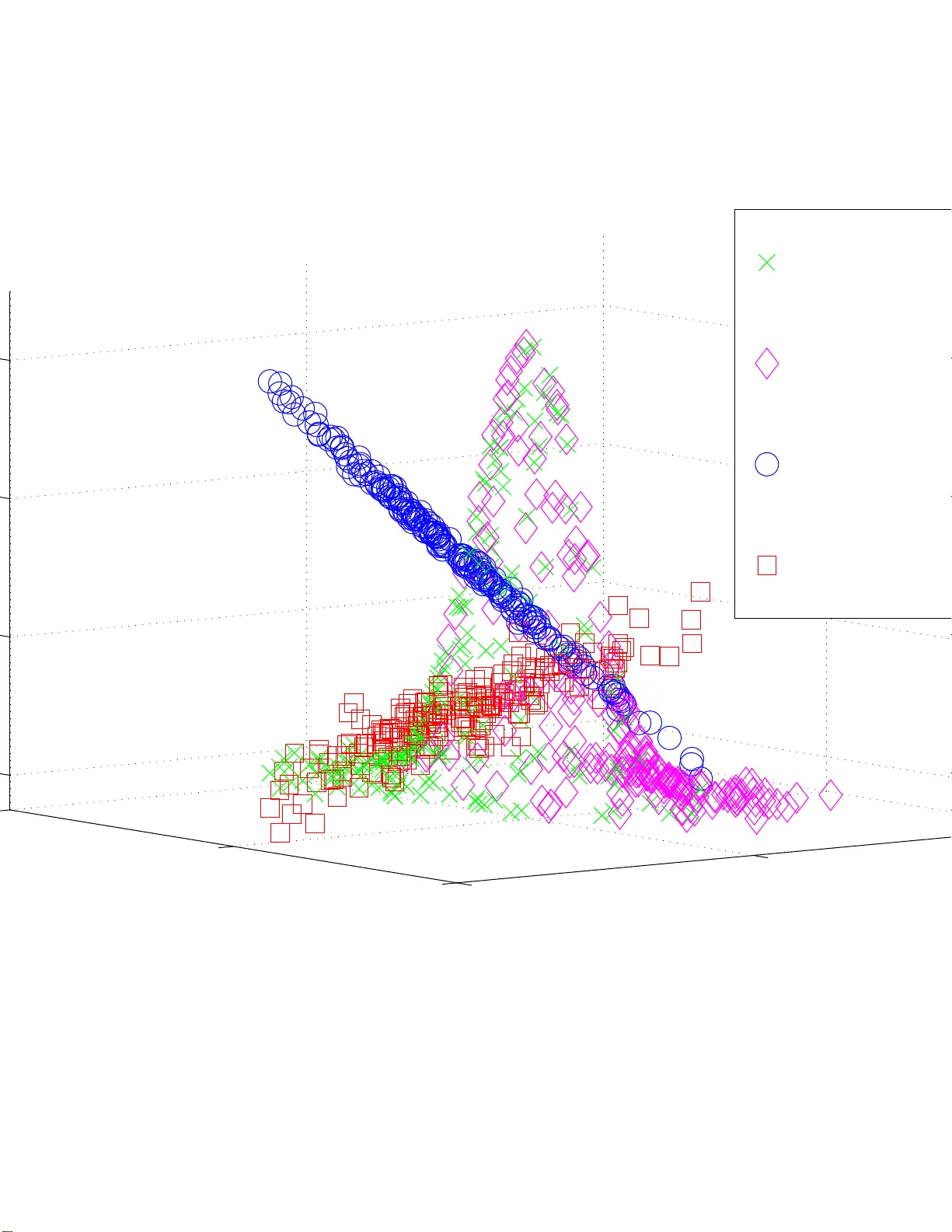
Domain Adaptation: Learn ing Bounds and Algorithms Y ishay Mansour Google Research and T el A viv Univ . mansour@tau.a c.il Mehryar Mohri Courant Institute and Google Research mohri@cims.ny u.edu Afshin Rostamizadeh Courant Institute New Y ork Univ ersity rostami@cs.ny u.edu Abstract This pa per addresses the g eneral pr oblem of do- main adap tation which arises in a variety of appli- cations w h ere the distribution o f th e labeled sam- ple av ailable somewhat dif fers from that of the test data. Building on previous work by Ben-David et al. (2007 ), we introduce a n ovel distance be- tween distributions, discr epancy d istance , that is tailored to ada p tation prob lems with arb itrary loss function s. W e giv e Rademacher complexity bounds for estimating the discrepa ncy distance from finite samples for different loss functions. Using this dis- tance, we derive nov el generalizatio n bound s for domain adap tation fo r a wide family of loss func- tions. W e a lso present a series o f novel a daptation bound s for large classes o f r egularization-b ased al- gorithms, including sup port vector machine s and kernel rid ge regression based on the empirical dis- crepancy . T his motiv ates our analysis of th e prob - lem of min imizing the empirical discrepan cy for various lo ss fu nctions for wh ich we also give n ovel algorithm s. W e rep ort the r e sults of p reliminary experiments that d e monstrate th e b enefits of our discrepancy min imization alg orithms for domain adaptation . 1 Intr oduction In the standard P AC mod el (V alian t, 1984) and other the- oretical mod els of learn ing, trainin g a nd test in stances ar e assumed to b e drawn from the same d istribution. This is a natural assumptio n since, wh en the training and test distri- butions substantially d iffer , th ere c an b e no ho pe f o r gen- eralization. Howe ver , in practice, there are several crucial scenarios where th e two distributions are more similar and learning can be mor e effective. On e such scenario is th at of domain adap tation , the main topic of ou r analysis. The pro blem of do main ad a ptation arises in a variety of applications in natu ral langu a g e p rocessing ( D r edze et al., 2007; Blitzer et a l. , 200 7; Jiang & Zh ai, 20 07; Chelb a & Acero, 200 6; Daum ´ e I II & Marcu, 200 6), speech p r ocessing (Legetter & W oodland, 1 995; Gau vain & Ch in -Hui, 19 94; Pietra et al., 199 2; Rosenf eld, 1996; Jelinek, 1998 ; Roark & Bacchiani, 200 3), compu ter vision (Mart´ ınez, 20 0 2), and many other areas. Quite often, little or no lab eled data is av ailable fr om the tar get do main , but lab eled d ata from a sour ce domain somewhat similar to the target as well a s large amounts of unlabeled data from the target domain are at one’ s disposal. The do main ad aptation p roblem then co nsists o f lev eraging th e source labeled and target unlabeled data to derive a hypoth esis p erform in g well on the target do main. A numb er o f different adap tation techniqu es have bee n introdu c ed in the past by the p u blications just m entioned and o ther similar work in the co ntext of specific app lica- tions. For example, a standar d tech nique used in statistical languag e modelin g and other gener ativ e models for part- of- speech tagging or parsing is based on th e maximu m a po s- teriori adaptatio n which uses the source data as prior knowl- edge to estimate th e mo del p arameters ( Roark & Bacchian i, 2003) . Similar tech n iques and other more refined o nes h av e been used fo r training max imum entropy models for lan - guage mod eling or co nditiona l m odels (Pietra et al., 199 2; Jelinek, 1998; Chelba & Acer o, 20 0 6; Da um ´ e III & Marcu, 2006) . The first theoretical an alysis of the d o main adaptation problem was presented by Ben -David et al. (2007) , wh o gave VC-dimension-b ased g eneralization boun ds for adap - tation in classification tasks. Perhaps, the m ost sign ifican t contribution of this work was th e definition and application of a distance betwe en distributions, th e d A distance, that is particularly relev ant to th e problem of domain adaptation and that can be estimated from finite sam ples fo r a finite VC di- mension, as previously shown by Kifer et al. (200 4). This work was later extend ed b y Blitzer et al. (2008 ) wh o also gave a boun d o n the erro r rate of a hypoth esis derived fro m a weighted co mbination of the source da ta sets for the specific case of empirical r isk minim ization. A theoretical study of domain adap tation was p r esented by Mansour et a l. ( 2009) , where the analy sis deals with the related but distinct case o f adaptation with mu ltiple sources, and wh e re the target is a mixture of the source distributions. This paper p resents a novel theoretical and alg orithmic analysis of the problem of domain ad aptation. It builds on the work of Ben-David et al. (2007 ) an d extend s it in se v- eral ways. W e introdu ce a novel distanc e , the discrepancy distance , th at is tailored to com paring distributions in a dap- tation. This distan c e coincides with the d A distance for 0-1 classification, but it c an be used to co mpare distributions for more gen eral tasks, includin g regression , and with other loss function s. As already pointed out, a crucial advantage of the d A distance is that it can b e estimated fr om finite samples when the set of region s used has finite VC-dim e nsion. W e prove that the same ho lds for the discre p ancy distance and in fact g iv e d ata-depen dent versions o f that stateme nt with sharper bound s based on the Rademache r comp lexity . W e g iv e new gener alization bo unds fo r dom ain ad apta- tion and p o int out some of their benefits by co mparin g them with previous b ound s. W e furth e r co mbine th ese with th e proper ties of the discrepa n cy distance to derive data-depen dent Rademacher com plexity learning boun d s. W e a lso pr esent a series o f novel results fo r large cla sses of regularization - based algorithm s, including sup port vector mac h ines ( SVMs) (Cortes & V apn ik, 1995 ) and kernel ridg e regression (KRR) (Saunder s et al., 1 998) . W e comp are th e po intwise loss of the hypoth esis return ed by these algorith ms when tra in ed o n a sample d rawn from the target do main distribution, versus that of a hypoth esis selected b y these algorithm s wh en tr a in - ing on a sample drawn from the sour ce distribution. W e show that th e difference of the se po in twise losses can be bo unded by a term that depends directly on the empirical discrepancy distance of the source and target distributions. These lear ning bo unds motivate the idea of replacing th e empirical source distribution with another distribution with the same supp ort but with th e smallest discrepan cy with re- spect to the target empir ical distribution, which can be viewed as reweighting the loss on each lab e le d p oint. W e analyz e the p r oblem of determinin g th e distribution m inimizing th e discrepancy in both 0 -1 classification and square loss regres- sion. W e show how the prob lem can be ca st as a linear pro- gram (LP) fo r the 0-1 loss and de riv e a specific efficient com- binatorial algo rithm to solve it in dimension on e. W e also giv e a p olynom ial-time a lgorithm for solving this prob lem in the case of the squ a r e loss by proving that it can b e cast as a semi-d efinite p rogra m (SDP). Finally , we repor t the re- sults of pr e liminary exper im ents showing th e benefits of our analysis and discrepan cy m in imization algo rithms. In section 2, we describe the learn ing set-up for domain adaptation a nd introdu ce the no tation and Radem acher com - plexity con cepts needed for the p resentation of our results. Section 3 in troduce s th e discrep ancy distance and a nalyzes its p roperties. Section 4 presents our g e neralization bo unds and o ur th eoretical guarantee s fo r regular ization-b a sed algo - rithms. Section 5 describ es and a nalyzes our discrep ancy minimization a lgorithms. Section 6 repo rts th e results of o u r preliminar y experiments. 2 Pr eliminaries 2.1 Learning Set-U p W e consider the familiar supervised lear n ing setting where the learn ing algo r ithm receives a sample of m labeled points S = ( z 1 , . . . , z m ) = (( x 1 , y 1 ) , . . . , ( x m , y m )) ∈ ( X × Y ) m , where X is the in put space and Y the label set, which is { 0 , 1 } in classification and some measurab le subset of R in regression. In the doma in ada ptation pr oblem , the training sample S is dr awn acc ording to a sour ce distribution Q , while test points are drawn a c cording to a tar get distribution P th at may somewhat d iffer f rom Q . W e deno te b y f : X → Y the target labeling function . W e shall also discuss cases where the so u rce labelin g fun ction f Q differs from th e target d o - main labeling fu nction f P . Clearly , this dissimilarity will need to be small for adaptation to be possible. W e will assume that the learner is p rovided with an unla- beled samp le T dr awn i.i.d. acco rding to the target distribu- tion P . W e denote b y L : Y × Y → R a lo ss fu nction d efined over p airs of labels and b y L Q ( f , g ) the expec te d loss for any two fun c tions f , g : X → Y and any distribution Q over X : L Q ( f , g ) = E x ∼ Q [ L ( f ( x ) , g ( x ))] . The domain adaptation prob lem consists of selecting a hypoth esis h out o f a h ypoth esis set H with a small expected loss accordin g to the target d istribution P , L P ( h, f ) . 2.2 Rademacher Co mplexity Our gener alization boun ds will be b a sed on the following data-dep e ndent measure of th e complexity of a class of func - tions. Definition 1 (Rademacher Complexity) Let H b e a set of r eal-valued fu nctions defined over a set X . Given a sam- ple S ∈ X m , the em p irical Ra demacher comp lexity o f H is defined as follows: b R S ( H ) = 2 m E σ h sup h ∈ H   m X i =1 σ i h ( x i )      S = ( x 1 , . . . , x m ) i . (1) The expectation is taken over σ = ( σ 1 , . . . , σ n ) wher e σ i s ar e in d epende nt unifo rm random va riables ta king valu es in {− 1 , +1 } . The Ra demacher c o mplexity of a hypo thesis set H is d efined a s the expectation of b R S ( H ) over all samples of size m : R m ( H ) = E S  b R S ( H )   | S | = m  . (2) The Rademac her com plexity measure s the ab ility of a class of function s to fit n oise. Th e empirical Rade macher c om- plexity has the a d ded advantage that it is d ata-depen dent and can b e measu red fro m finite sam ples. I t can lead to tighter bound s than those based on o ther mea su res of complexity such as the VC-dimension (K oltchinskii & Panchen ko, 2 0 00). W e will deno te by b R S ( h ) the empir ical average of a hy - pothesis h : X → R and by R ( h ) its expectatio n over a sample S drawn accordin g to the distribution consider ed. The f ollowing is a version of th e Radem acher complexity bound s by Koltchinskii an d Panchenko ( 2000 ) and Bartlett and Mendelson (2 002) . For com pleteness, the f ull proof is giv en in the App endix. Theorem 2 (Radema c her Bo und) Let H b e a class of fu n c- tions ma pping Z = X × Y to [0 , 1] a nd S = ( z 1 , . . . , z m ) a fi n ite samp le drawn i.i.d. acco r ding to a distribution Q . Then, for any δ > 0 , with pr obability at lea st 1 − δ over samples S of size m , the follo wing in equality holds for all h ∈ H : R ( h ) ≤ b R ( h ) + b R S ( H ) + 3 s log 2 δ 2 m . (3) 3 Distances between Distributions Clearly , f o r g eneralization to be possible, the distribution Q and P m u st no t be too dissimilar, thu s so me measur e of the similarity of these distributions will be critical in the deriv a- tion o f our generaliza tion bound s or the design of ou r algo- rithms. This sectio n d iscusses this q uestion and introdu ces a discr epancy d istance relev ant to the context o f adaptation. The l 1 distance yields a straig htforward bound on the d if- ference of the error of a hypo thesis h with respect to Q versus its error with respect to P . Proposition 1 Assume th at the loss L is bou n ded, L ≤ M for some M > 0 . Then, for any hy p othesis h ∈ H , |L Q ( h, f ) − L P ( h, f ) | ≤ M l 1 ( Q, P ) . (4) This provides us with a first adaptation bo u nd sugg esting that f or small values of the l 1 distance betwee n the sou rce and target distributions, the average loss of hypo thesis h tested on the target domain is clo se to its average loss o n the source domain. Howe ver , in general, th is b ound is no t info rmative since the l 1 distance can be large even in fav orable adaptation situations. Instead , o ne c a n u se a distance between distribu- tions better suited to the learnin g task. Consider for example the case of classification with the 0-1 loss. Fix h ∈ H , and let a denote the suppor t of | h − f | . Observe that |L Q ( h, f ) − L P ( h, f ) | = | Q ( a ) − P ( a ) | . A natural distance between distributions in this con text is th us one based on the supr e mum of the right-h and side over all regions a . Since the target hy pothesis f is no t known, the region a shou ld be taken as the support of | h − h ′ | for any two h, h ′ ∈ H . This leads us to the fo llowing definition of a distance originally introdu c e d b y Devroye et al. ( 1996) [pp. 27 1 - 272] un der the name of generalized K olmogor ov-S mirnov distance , later by Kifer et al. (2004 ) as the d A distance , and introd u ced and applied to the analysis of adaptatio n in classification by Ben-David et al. ( 2007) and Blitzer et al. (2008 ). Definition 3 ( d A -Distance) Let A ⊆ 2 | X | be a set of sub sets of X . Th en, the d A -distance between two distributions Q 1 and Q 2 over X , is defin ed a s d A ( Q 1 , Q 2 ) = sup a ∈ A | Q 1 ( a ) − Q 2 ( a ) | . (5) As just d iscussed, in 0-1 c la ssification , a natur al cho ice for A is A = H ∆ H = {| h ′ − h | : h, h ′ ∈ H } . W e intro duce a distance between d istributions, discr epancy distance , that can be used to comp are d istributions fo r m ore general tasks, e.g., regression. Our cho ice of the terminolog y is par tly mo - ti vated by the relation ship of this notion with th e discrep ancy problem s arising in com binatorial co ntexts (Chazelle, 2000). Definition 4 (Discrepancy Dista nce) Let H be a set of func- tions mappin g X to Y a nd let L : Y × Y → R + define a loss function over Y . The discr epancy distan ce dis c L between two distributions Q 1 and Q 2 over X is d efined b y disc L ( Q 1 , Q 2 ) = max h,h ′ ∈ H    L Q 1 ( h ′ , h ) − L Q 2 ( h ′ , h )    . The d iscrepancy distanc e is clearly symmetric and it is no t hard to verify that it verifies th e triangle in equality , regard - less of the loss f unction u sed. I n general, however , it does not define a distance : we may h ave disc L ( Q 1 , Q 2 ) = 0 fo r Q 1 6 = Q 2 , e ven for non-trivial hypo thesis sets such as that o f bound ed linear fun ctions an d standard continu o us loss fu nc- tions. Note th at for the 0-1 classification loss, the discrepan cy distance coin cides with the d A distance with A = H ∆ H . But the discrep ancy distance helps u s compar e distributions for other losses such as L q ( y , y ′ ) = | y − y ′ | q for some q and is more general. As shown by Kifer et al. (20 04), an impo rtant ad van- tage of the d A distance is that it can be estimated fr o m finite samples wh en A has finite VC-dimen sio n. W e pr ove that the same holds for the disc L distance and in fact give data- depend ent versions of that statement with sharper bou nds based on the Rademach e r complexity . The fo llowing th eorem shows that for a boun ded loss function L , the discrepan cy distan ce disc L between a distri- bution and its empirical distribution can b e bo unded in terms of the empirical Rademach er complexity of the c la ss of func- tions L H = { x 7→ L ( h ′ ( x ) , h ( x )) : h, h ′ ∈ H } . In par ticu- lar , when L H has finite pseud o-dimen sion, this imp lies that the discrepancy distan c e con verges to zer o as O ( p log m/m ) . Proposition 2 Assume that the lo ss functio n L is b o unded by M > 0 . Let Q be a distribution over X and let b Q deno te the co rr esponding empirical distribution fo r a samp le S = ( x 1 , . . . , x m ) . Then, fo r any δ > 0 , with pr obability at lea st 1 − δ over samp le s S of size m drawn according to Q : disc L ( Q, b Q ) ≤ b R S ( L H ) + 3 M s log 2 δ 2 m . (6) Proof: W e scale the loss L to [0 , 1] by dividing by M , and denote th e new class b y L H / M . By Theorem 2 applied to L H / M , fo r any δ > 0 , with probability at least 1 − δ , th e following inequ ality holds for all h, h ′ ∈ H : L Q ( h ′ , h ) M ≤ L b Q ( h ′ , h ) M + b R S ( L H / M ) + 3 s log 2 δ 2 m . The emp irical Rademacher com plexity has the p roperty that b R ( αH ) = α b R ( H ) for any h ypothe sis class H and pos- iti ve re al number α (Bartlett & Mendelson , 200 2). Th us, R S ( L H / M ) = 1 M R S ( L H ) , which pr oves the p roposition . For the specific case of L q regression lo sses, th e boun d can be made more explicit. Corollary 5 Let H be a hypo thesis set bounde d by some M > 0 for the lo ss functio n L q : L q ( h, h ′ ) ≤ M , for all h, h ′ ∈ H . Let Q b e a distribution over X and let b Q de- note the corresponding empirical distribution for a sample S = ( x 1 , . . . , x m ) . Then, for any δ > 0 , with pr obability at least 1 − δ over samples S of size m drawn according to Q : disc L q ( Q, b Q ) ≤ 4 q b R S ( H ) + 3 M s log 2 δ 2 m . (7) Proof: The function f : x 7→ x q is q -Lipschitz for x ∈ [0 , 1] : | f ( x ′ ) − f ( x ) | ≤ q | x ′ − x | , (8) and f (0) = 0 . For L = L q , L H = { x 7→ | h ′ ( x ) − h ( x ) | q : h, h ′ ∈ H } . Th us, by T alag rand’ s contractio n lem ma (Ledou x & T alagrand, 199 1), b R ( L H ) is bounde d by 2 q b R ( H ′ ) with H ′ = { x 7→ ( h ′ ( x ) − h ( x )) : h, h ′ ∈ H } . Then, b R S ( H ′ ) can be written and bou nded as f ollows b R S ( H ′ ) = E σ  sup h,h ′ 1 m | m X i =1 σ i ( h ( x i ) − h ′ ( x i )) |  ≤ E σ [sup h 1 m | m X i =1 σ i h ( x i ) | ] + E σ [sup h ′ 1 m | m X i =1 σ i h ′ ( x i ) | ] = 2 b R S ( H ) , using the definition of the Rad e m acher variables and the su b - additivity o f the supremu m f unction. This proves the in- equality b R ( L H ) ≤ 4 q b R ( h ) an d the corollary . A very similar p r oof gives the following r esult for classi- fication. Corollary 6 Let H be a set of classifiers mapping X to { 0 , 1 } and let L 01 denote th e 0-1 lo ss. Then, with the notatio n o f Cor olla ry 5, for an y δ > 0 , with p r ob ability at least 1 − δ over samp le s S of size m drawn according to Q : disc L 01 ( Q, b Q ) ≤ 4 b R S ( H ) + 3 s log 2 δ 2 m . (9) The factor o f 4 can in fact b e r e duced to 2 in th ese corollar- ies when using a more fav orable con stant in the c o ntraction lemma. The f ollowing corollar y shows that the discrepa n cy distance can be estimated from finite samples. Corollary 7 Let H be a hypo thesis set bounde d by some M > 0 fo r the loss function L q : L q ( h, h ′ ) ≤ M , for all h, h ′ ∈ H . Let Q be a distrib ution over X a n d b Q the cor- r esponding empirical distribution for a sample S , a nd let P be a d istrib ution over X an d b P the co rr esponding empiri- cal distribution for a sam p le T . Then, fo r any δ > 0 , with pr o bability at least 1 − δ over samples S o f size m drawn according to Q and samples T o f size n drawn accor ding to P : disc L q ( P, Q ) ≤ disc L q ( b P , b Q )+ 4 q  b R S ( H )+ b R T ( H )  + 3 M s log 4 δ 2 m + s log 4 δ 2 n ! . Proof: By th e tr iangle inequality , we can write disc L q ( P, Q ) ≤ disc L q ( P, b P ) + disc L q ( b P , b Q )+ disc L q ( Q, b Q ) . (10) The result then follows by the application of Coro llary 5 to disc L q ( P, b P ) and disc L q ( Q, b Q ) . As with Coro llary 6, a similar resu lt hold s for the 0-1 lo ss in classification. 4 Domain Adaptation: G eneralization Bounds This section presents generalization bounds for d omain adap- tation g iv en in terms of the discrepa n cy distance just defined. In the context of ad aptation, two ty p es o f questions arise: (1) we m ay ask, as for standar d gen eralization, how the av erage loss of a h ypothesis on the target distribution, L P ( h, f ) , differs f r om L b Q ( h, f ) , its empirical error based on the empirical distribution b Q ; (2) another natural question is, given a specific learnin g al- gorithm, by how mu c h does L P ( h Q , f ) d eviate from L P ( h P , f ) where h Q is the h y pothesis retu rned by the algorithm when tr ained on a sample drawn from Q a nd h P the one it would have retur ned by training on a sam- ple drawn fro m the true target distribution P . W e will p r esent theo retical g uarantee s ad dressing both qu es- tions. 4.1 Generalizatio n bounds Let h ∗ Q ∈ arg min h ∈ H L Q ( h, f Q ) a n d similarly let h ∗ P be a minimizer of L P ( h, f P ) . Note that these m inimizers may not be unique. For ad aptation to suc ceed, it is n atural to assume th at the av erage loss L Q ( h ∗ Q , h ∗ P ) between the best- in-class hypo theses is small. Un der that assum ption and fo r a small discrepancy d istance, th e following theor e m provides a useful b o und o n th e error of a hyp othesis with respect to the target d omain. Theorem 8 Assume that the lo ss fun ction L is symmetric and obeys th e triangle inequ ality . Then, for any h ypothesis h ∈ H , the following holds L P ( h, f P ) ≤ L P ( h ∗ P , f P ) + L Q ( h, h ∗ Q ) + disc L ( P, Q ) + min {L Q ( h ∗ Q , h ∗ P ) , L P ( h ∗ Q , h ∗ P ) } . (11) Proof: W e show two inequalities, th e combin ation of which proves th e theorem . Fix h ∈ H . By the trian gle in equality proper ty of L and the definition of the discrepancy disc L ( P, Q ) , the following hold s L P ( h, f P ) ≤ L P ( h, h ∗ Q ) + L P ( h ∗ Q , h ∗ P ) + L P ( h ∗ P , f P ) ≤ L Q ( h, h ∗ Q ) + disc L ( P, Q ) + L P ( h ∗ Q , h ∗ P ) + L P ( h ∗ P , f P ) . Similarly , using same arguments, we have L P ( h, f P ) ≤ L P ( h, h ∗ P ) + L P ( h ∗ P , f P ) ≤ L Q ( h, h ∗ P ) + disc L ( P, Q ) + L P ( h ∗ P , f P ) ≤ L Q ( h, h ∗ Q ) + L Q ( h ∗ Q , h ∗ P ) + disc L ( P, Q ) + L P ( h ∗ P , f P ) . W e comp a re (11 ) with the main adaptation boun d given by Ben-David et al. (2007) and Blitzer et al. (200 8): L P ( h, f P ) ≤ L Q ( h, f Q ) + disc L ( P, Q )+ min h ∈ H  L Q ( h, f Q ) + L P ( h, f P )  . (12) It is very instru ctiv e to com pare the two boun d s. Intuitively , the b o und of T h eorem 8 has o nly on e error ter m that in volves the target fun c tion, while the boun d of (12) ha s three ter ms in volving the target function . One extreme case is when there is a sing le hy pothesis h in H and a sing le target fu nction f . In this case, The o rem 8 gives a b ound of L P ( h, f ) + disc( P, Q ) , while the boun d sup plied by (12 ) is 2 L Q ( h, f ) + L P ( h, f ) + disc( P , Q ) , which is larger than 3 L P ( h, f ) + disc( P, Q ) when L Q ( h, f ) ≤ L P ( h, f ) . One can even see that the bound of (12 ) mig ht becom e vacuous fo r mod erate values of L Q ( h, f ) and L P ( h, f ) . While this is clearly an extreme case, an error with a factor of 3 can arise in more realistic situations, especially when the distance between th e target fun ction an d th e hypo thesis class is significant. While in g eneral the two b o unds are inc omparab le, it is worthwh ile to compar e them using som e relatively p lau- sible assum ptions. Assume that the discr epancy d istance between P a nd Q is small and so is the average lo ss be- tween h ∗ Q and h ∗ P . These are natura l assumptions f o r ad ap- tation to be possible. Then, Theo rem 8 ind icates that the regret L P ( h, f P ) − L P ( h ∗ P , f P ) is e ssentially bo unded b y L Q ( h, h ∗ Q ) , the av erage loss with respect to h ∗ Q on Q . W e now consid er several special cases of interest. (i) When h ∗ Q = h ∗ P then h ∗ = h ∗ Q = h ∗ P and the boun d of Theorem 8 becom e s L P ( h, f P ) ≤ L P ( h ∗ , f P ) + L Q ( h, h ∗ ) + disc( P, Q ) . (13) The boun d of (12) becom es L P ( h, f P ) ≤ L P ( h ∗ , f P ) + L Q ( h, f Q )+ L Q ( h ∗ , f Q ) + disc( P, Q ) , where the right-h and side essentially inclu des the sum of 3 erro rs and is always larger than the righ t- hand side of (13) since by the triangle inequ a lity L Q ( h, h ∗ ) ≤ L Q ( h, f Q ) + L Q ( h ∗ , f Q ) . (ii) When h ∗ Q = h ∗ P = h ∗ ∧ disc( P , Q ) = 0 , the bound o f Theorem 8 becom e s L P ( h, f P ) ≤ L P ( h ∗ , f P ) + L Q ( h, h ∗ ) , which coincides with the standard generalization bound. The bound o f (1 2) does not coincide with the standar d bound and leads to: L P ( h, f P ) ≤ L P ( h ∗ , f P ) + L Q ( h, f Q ) + L Q ( h ∗ , f Q ) . (iii) When f P ∈ H (co nsistent case), th e boun d o f (12) sim- plifies to, |L P ( h, f P ) − L Q ( h, f P ) | ≤ disc L ( Q, P ) , and it can also b e d erived using the proo f of The orem 8. Finally , clearly Theor em 8 leads to bound s based on the em- pirical erro r o f h on a sample drawn accor d ing to Q . W e giv e the boun d related to th e 0-1 loss, others can be derived in a similar way f rom Corollaries 5-7 and o ther similar corol- laries. T he result follows Theo r em 8 co mbined with Cor ol- lary 7, an d a standard Rademach er classification bound (The- orem 14) (Bartlett & Mend e lson, 200 2). Figure 1: In this example, the gray regions are assumed to have zero sup port in th e target distribution P . Thus, ther e exist con sistent hypo th eses such as the linea r separator dis- played. Howe ver , f or th e sou rce d istribution Q no linear sep- aration is possible. Theorem 9 Let H be a family of fun ctions map ping X to { 0 , 1 } and let the rest of the assumptio ns be a s in Cor o l- lary 7. Th en, for a n y hypo thesis h ∈ H , with pr obability at least 1 − δ , the following a daptatio n generalization bou nd holds for the 0-1 loss: L P ( h, f P ) − L P ( h ∗ P , f P ) ≤ L b Q ( h, h ∗ Q )+ disc L 01 ( b P , b Q ) + (4 q + 1 2 ) b R S ( H )+ 4 q b R T ( H )+ 4 s log 8 δ 2 m + 3 s log 8 δ 2 n + L Q ( h ∗ Q , h ∗ P ) . (14) 4.2 Guarantees for regularizatio n-based alg orithms In this section , we first assume that the h y pothesis set H in - cludes the target fun ction f P . N o te that this does no t imply that f Q is in H . Even when f P and f Q are restriction s to supp( P ) and supp( Q ) of the same labeling fun c tion f , we may have f P ∈ H and f Q 6∈ H and the source pro blem could be non-re alizable. Figur e 1 illu strates th is situation. For a fixed loss f unction L , we den ote by R b Q ( h ) the em- pirical error of a hyp othesis h with respect to an empir ical distribution b Q : R b Q ( h ) = L b Q ( h, f ) . Let N : H → R + be a fu nction d efined over the hypo thesis set H . W e will as- sume that H is a conve x subset of a vector space and that the loss fun ction L is con vex with re sp ect to each of its argu- ments. Regular ization-based algor ith ms minimize an obje c - ti ve of th e fo rm F b Q ( h ) = b R b Q ( h ) + λN ( h ) , (15) where λ ≥ 0 is a trade-off p arameter . This family of al- gorithms includes suppor t vector machines ( SVM) (Cortes & V ap n ik, 19 95), suppo rt vector regre ssion (SVR) (V apn ik, 1998) , kern el ridge regression (Saunde r s et al., 199 8), and other algorith ms such as those based on the r elativ e entropy regularization ( Bo usquet & E lisseef f, 2002) . W e deno te by B F the Bregman d iv ergence associated to a conve x fun ction F , B F ( f k g ) = F ( f ) − F ( g ) − h f − g , ∇ F ( g ) i (16) and define ∆ h as ∆ h = h ′ − h . Lemma 10 Let th e h ypothesis set H be a vector sp ace. As- sume tha t N is a pr oper closed conve x fun c tion and th at N and L ar e differ entiable. Assume that F b Q admits a minimizer h ∈ H and F b P a minimizer h ′ ∈ H and that f P and f Q co- incide on th e supp ort of b Q . Then, th e following bound holds, B N ( h ′ k h ) + B N ( h k h ′ ) ≤ 2disc L ( b P , b Q ) λ . (17) Proof: Since B F b Q = B b R b Q + λB N and B F b P = B b R b P + λB N , and a Bregman diver gence is n on-negative, the f ollowing in - equality holds: λ  B N ( h ′ k h ) + B N ( h k h ′ )  ≤ B F b Q ( h ′ k h ) + B F b P ( h k h ′ ) . By the definition of h and h ′ as the minimizers of F b Q and F b P , ∇ b Q F ( h ) = ∇ b P F ( h ′ ) = 0 and λ  B F b Q ( h ′ k h ) + B F b P ( h k h ′ )  = b R b Q ( h ′ ) − b R b Q ( h ) + b R b P ( h ) − b R b P ( h ′ ) =  L b P ( h, f P ) − L b Q ( h, f P )  −  L b P ( h ′ , f P ) − L b Q ( h ′ , f P )  ≤ 2disc L ( b P , b Q ) . This last ineq uality holds sinc e b y assumption f P is in H . W e will say that a loss function L is σ -admissible wh en there exists σ ∈ R + such th at fo r any two hyp otheses h, h ′ ∈ H and for all x ∈ X , and y ∈ Y ,   L ( h ( x ) , y ) − L ( h ′ ( x ) , y )   ≤ σ   h ( x ) − h ′ ( x )   . (18) This assumption ho lds for the hinge loss with σ = 1 an d for the L q loss with σ = q (2 M ) q − 1 when th e hypoth e sis set and the set of ou tput labels are bo unded by some M ∈ R + : ∀ h ∈ H , ∀ x ∈ X , | h ( x ) | ≤ M and ∀ y ∈ Y , | y | ≤ M . Theorem 11 Let K : X × X → R be a positive- d efinite sym- metric kernel such that K ( x, x ) ≤ κ 2 < ∞ for all x ∈ X , and let H be th e repr oducin g kernel Hilb ert space associ- ated to K . A ssume that the loss func tion L is σ -ad missible. Let h ′ be the hypothesis r eturned b y the r egularization a lgo- rithm ba sed on N ( · ) = k·k 2 K for the empirical d istribution b P , and h the one r eturned for the empirica l distribution b Q , and that and tha t f P and f Q coincide on supp( b Q ) . Then, for all x ∈ X , y ∈ Y ,   L ( h ′ ( x ) , y ) − L ( h ( x ) , y )   ≤ κσ s disc L ( b P , b Q ) λ . (19) Proof: For N ( · ) = k·k 2 K , N is a prop er closed conve x func- tion an d is differentiable. W e hav e B N ( h ′ k h ) = k h ′ − h k 2 K , thus B N ( h ′ k h ) + B N ( h k h ′ ) = 2 k ∆ h k 2 K . When L is differ - entiable, by Lemma 10, 2 k ∆ h k 2 K ≤ 2disc L ( b P , b Q ) λ . ( 20) This result can also be shown directly without assum ing that L is d ifferentiable b y using the conv exity of N and the mini- mizing pr o perties of h and h ′ with a proof that is lon g er th an that of Lemma 10. Now , by the rep roduc ing pr o perty o f H , for all x ∈ H , ∆ h ( x ) = h ∆ h, K ( x, · ) i and b y the Cauch y-Schwarz in- equality , | ∆ h ( x ) | ≤ k ∆ h k K ( K ( x, x )) 1 / 2 ≤ κ k ∆ h k K . By the σ -admissibility of L , fo r all x ∈ X , y ∈ Y , | L ( h ′ ( x ) , y ) − L ( h ( x ) , y ) | ≤ σ | ∆ h ( x ) | ≤ κσ k ∆ h k K , which, comb in ed with ( 20), p roves the stateme n t o f the the- orem. Theorem 11 provides a g uarantee o n the pointwise dif- ference of the loss for h ′ and h with probab ility o ne, which of course is stronger th a n a bo und on th e difference be tween expected lo sses or a prob abilistic statemen t. The result, as well as the proof , also sugg ests that the d iscrepancy distance is the “right” measure of difference of distributions for th is context. Th e theore m applies to a variety of algorithms, in particular SVMs com bined with arbitr a ry PDS kernels and kernel rid ge regression. In g eneral, the functions f P and f Q may not coincide on supp( b Q ) . For adaptation to be possible, it is r easonable to assume howe ver that L b Q ( f Q ( x ) , f P ( x )) ≪ 1 and L b P ( f Q ( x ) , f P ( x )) ≪ 1 . This can be v iewed as a condition o n the prox imity o f the labeling function s (the Y s), while the discrepancy d istan ce relates to the d istributions on th e input space (the X s). The following result g e neralizes T heorem 11 to this setting in the case of the square loss. Theorem 12 Un der the assumptions of Theor em 11 , but with f Q and f P potentially d iffer en t on supp( b Q ) , when L is th e squar e loss L 2 and δ 2 = L b Q ( f Q ( x ) , f P ( x )) ≪ 1 , the n, for all x ∈ X , y ∈ Y ,   L ( h ′ ( x ) , y ) − L ( h ( x ) , y )   ≤ 2 κM λ  κδ + q κ 2 δ 2 + 4 λ disc L ( b P , b Q )  . (21) Proof: Proceeding as in the proo f of Le m ma 1 0 an d u sing the definition of the square loss and th e Cauchy-Schwarz in- equality giv e λ  B F b Q ( h ′ k h ) + B F b P ( h k h ′ )  = b R b Q ( h ′ ) − b R b Q ( h ) + b R b P ( h ) − b R b P ( h ′ ) =  L b P ( h, f P ) − L b Q ( h, f P )  −  L b P ( h ′ , f P ) − L b Q ( h ′ , f P )  + 2 E b Q [( h ′ ( x ) − h ( x ))( f P ( x ) − f Q ( x )] ≤ 2disc L ( b P , b Q ) + 2 r E b Q [∆ h ( x ) 2 ] E b Q [ L ( f P ( x ) , f Q ( x ))] ≤ 2disc L ( b P , b Q ) + 2 κ k ∆ h k K δ. Since N ( · ) = k·k 2 K , the inequa lity can be rewritten as λ k ∆ h k 2 K ≤ disc L ( b P , b Q ) + κδ k ∆ h k K . (22) Solving th e secon d-degree p olyno mial in k ∆ h k K leads to the equiv alent con straint k ∆ h k K ≤ 1 2 λ  κδ + q κ 2 δ 2 + 4 λ disc L ( b P , b Q )  . (23) The result then follows by th e σ - admissibility of L as in the proof of Theorem 11, with σ = 4 M . Using the same proof schema, similar b ound s can be de- riv ed fo r other loss functions. When the assumption f P ∈ H is r elaxed, the following theorem holds. Theorem 13 Un der the assumptions of Theor em 11 , but with f P not nece ssarily in H an d f Q and f P potentially differ- ent on supp( b Q ) , when L is the squa r e loss L 2 and δ ′ = L b Q ( h ∗ P ( x ) , f Q ( x )) 1 / 2 + L b P ( h ∗ P ( x ) , f P ( x )) 1 / 2 ≪ 1 , then, for all x ∈ X , y ∈ Y ,   L ( h ′ ( x ) , y ) − L ( h ( x ) , y )   ≤ 2 κM λ  κδ ′ + q κ 2 δ ′ 2 + 4 λ disc L ( b P , b Q )  . (24) Proof: Pro ceeding as in th e proo f of Theor em 12 and us- ing the definition of the square loss an d the Cauchy -Schwarz inequality give λ  B F b Q ( h ′ k h ) + B F b P ( h k h ′ )  =  L b P ( h, h ∗ P ) − L b Q ( h, h ∗ P )  −  L b P ( h ′ , h ∗ P ) − L b Q ( h ′ , h ∗ P )  − 2 E b P [( h ′ ( x ) − h ( x ))( h ∗ P ( x ) − f P ( x )] + 2 E b Q [( h ′ ( x ) − h ( x ))( h ∗ P ( x ) − f Q ( x )] ≤ 2 disc L ( b P , b Q ) + 2 r E b P [∆ h ( x ) 2 ] E b P [ L ( h ∗ P ( x ) , f P ( x ))] + 2 r E b Q [∆ h ( x ) 2 ] E b Q [ L ( h ∗ P ( x ) , f Q ( x ))] ≤ 2 disc L ( b P , b Q ) + 2 κ k ∆ h k K δ ′ . The rest of the pro o f is identical to that o f Th eorem 1 2. 5 Discre pancy Minimization Algorithms The discrepan cy distance disc L ( b P , b Q ) appear ed as a critical term in several of the bou n ds in the last section. In par ticular , Theorem s 11 and 12 su g gest th at if we cou ld select, instead of b Q , som e other empirical distribution b Q ′ with a smaller empirical discrep ancy disc L ( b P , b Q ′ ) an d use that fo r train ing a regular ization-based algor ith m, a b etter guar antee would be obtained on the difference of pointwise loss betwee n h ′ and h . Sin ce h ′ is fixed, a sufficiently smaller discrepan cy would actu ally lead to a hy pothesis h with po intwise loss closer to that of h ′ . The trainin g sample is given and we do not have any con- trol over the sup port of b Q . Bu t, we can sear ch for the distri- bution b Q ′ with the minimal empirical discrepancy distanc e: b Q ′ = arg min b Q ′ ∈Q disc L ( b P , b Q ′ ) , (25) where Q denotes the set of distributions with suppor t supp( b Q ) . This lead s to a n optimiz a tion problem th at we shall study in detail in the case of sev eral loss functions. Note that using b Q ′ instead of b Q for training can be vie wed as r eweighting the cost of an erro r o n each tra ining po int. The distribution b Q ′ can be used to em phasize some points or d e-emph asize others to red u ce the emp irical d iscrepancy distance. This bear s some similarity with the r eweighting or importance weig hting idea s used in statistics and machin e learning f or samp le bias corr ection techn iques (Elkan , 2001 ; Cortes et al., 200 8 ) and o ther pu rposes. Of course, the o b- jectiv e o ptimized h ere based on the discrepancy distance is distinct from that of previous reweighting techn iques. W e will d e note by S Q the sup port of b Q , b y S P the sup- port of b P , and by S their unio n supp( b Q ) ∪ supp( b P ) , with | S Q | = m 0 ≤ m and | S P | = n 0 ≤ n . In vie w of th e definition of the discrepancy d istance, pro b - lem (25) can be written as a min-m ax prob lem: b Q ′ = a rgmin b Q ′ ∈Q max h,h ′ ∈ H |L b P ( h ′ , h ) − L b Q ′ ( h ′ , h ) | . (26) As with all min-max problem s, the pro blem has a natural game theore tica l interpre ta tio n. Howe ver , her e , in general, we cann o t perm ute the min and max operators since the conv exity-type assumptions of the minimax theorems do not hold. Nevertheless, since the max - min value is alw ays a lower bo und f or the m in-max, it p rovides us with a lower bound on the value of th e ga me, that is th e minimal discrep - ancy: max h,h ′ ∈ H min b Q ′ ∈Q |L b P ( h ′ , h ) − L b Q ′ ( h ′ , h ) | ≤ min b Q ′ ∈Q max h,h ′ ∈ H |L b P ( h ′ , h ) − L b Q ′ ( h ′ , h ) | . (27 ) W e will later make use of this inequality . Let us now examin e the m inimization problem (25) and its algorith mic solution s in the case o f classification with the 0-1 lo ss and r egression with the L 2 loss. 5.1 Classification, 0 -1 Loss For the 0-1 loss, the prob lem of finding the best distribution b Q ′ can be reform ulated as the following min- max p rogra m: min Q ′ max a ∈ H ∆ H   b Q ′ ( a ) − b P ( a )   (28) subject to ∀ x ∈ S Q , b Q ′ ( x ) ≥ 0 ∧ X x ∈ S Q b Q ′ ( x ) = 1 , (2 9) where we have iden tified H ∆ H = {| h ′ − h | : h, h ′ ∈ H } with the set of regions a ⊆ X that ar e the suppo rt of an element of H ∆ H . This pr oblem is similar to the min -max resource allocation problem that arises in task op tim ization (Karabati et al., 2001) . I t can b e rewritten a s th e following linear prog r am (LP): min Q ′ δ (30) subject to ∀ a ∈ H ∆ H, b Q ′ ( a ) − b P ( a ) ≤ δ (31) ∀ a ∈ H ∆ H, b P ( a ) − b Q ′ ( a ) ≤ δ (32) ∀ x ∈ S Q , b Q ′ ( x ) ≥ 0 ∧ X x ∈ S Q b Q ′ ( x ) = 1 . (3 3) The n umber of constraints is p ropor tional to | H ∆ H | but it can b e reduc ed to a finite number by observ ing th at two sub- sets a, a ′ ∈ H ∆ H con ta in ing th e same elements of S lead to redund ant constrain ts, since   b Q ′ ( a ) − b P ( a )   =   b Q ′ ( a ′ ) − b P ( a ′ )   . (34) (a) (b) Figure 2: Illustration of the discrepancy minimiza tio n algo- rithm in dimension one. (a) Sequ e nce o f labeled (red) and unlabeled (blue) points. ( b) The weight assigne d to each la- beled p oint is the su m of the weigh ts o f the con secutive blue points on its right. Thus, it suffices to keep one ca n onical memb er a fo r each such equivalence class. The necessary number of co nstraints to be c o nsidered is p ropor tional to Π H ∆ H ( m 0 + n 0 ) , the shattering co efficient of order ( m 0 + n 0 ) o f the hypothesis class H ∆ H . By the Sau er’ s lemma, this is bou nded in terms of the VC-dimensio n o f the class H ∆ H , Π H ∆ H ( m 0 + n 0 ) ≤ O (( m 0 + n 0 ) V C ( H ∆ H ) ) , which can be bo unded by O (( m 0 + n 0 ) 2 V C ( H ) ) since it is not har d to see th at V C ( H ∆ H ) ≤ 2 V C ( H ) . In cases where we can test efficiently whether there exists a co n sistent hy pothesis in H , e.g . , for half-spaces in R d , we can generate in time O (( m 0 + n 0 ) 2 d ) all consistent labeling of th e samp le po ints by H . (W e remark that co mputing the discrepancy with the 0-1 loss is closely related to agnostic learning. The imp lications of this fact will b e described in a longer version o f this p a per .) 5.2 Computing the Discrepancy in 1 D W e co nsider the case wher e X = [0 , 1] and d erive a simp le algorithm for m inimizing th e discrepan cy for 0-1 loss. Let H b e the class of all prefixes (i.e., [0 , z ] ) and su ffix es (i.e., [ z , 1] ) . Our class o f H ∆ H in cludes all the intervals (i. e., ( z 1 , z 2 ] ) and their complem ents (i.e., [0 , z 1 ] ∪ ( z 2 , 1] ) . W e start with a gener al lower b ound o n the discrepancy . Let U d enote th e set of un labeled r e gions , th at is the set of regions a such that a ∩ S Q = ∅ and a ∩ S P 6 = ∅ . If a is an unlabeled region, then | b Q ′ ( a ) − b P ( a ) | = b P ( a ) f o r any b Q ′ . Thus, by the ma x-min inequality (27), the fo llowing lower bound holds for the minimu m discrepan cy: max a ∈ U b P ( a ) ≤ min b Q ′ ∈Q max h,h ′ ∈ H |L b P ( h ′ , h ) − L b Q ′ ( h ′ , h ) | . (35) In particu lar , if there is a large un labeled region a , we cann ot hope to achieve a small empirical discrepancy . In the one-d imensional case, we giv e a simple linear-time algorithm that does not r e q uire an LP and show that the lower bound (35) is reac hed. Thus, in that ca se, the min a nd max operator s commu te and the min imal d iscrepancy distance is precisely min a ∈ U b P ( a ) . Giv en our definition of H , the u nlabeled regions are op en intervals, o r co m plements of these sets, containing only points from S P with endp oints defined by elemen ts of S Q . Let us den ote by s 1 , . . . , s m 0 the elemen ts o f S Q , b y n i , i ∈ [1 , m 0 ] , the numb er o f co nsecutive unlab eled poin ts to the rig ht of s i and n = P n i . W e will make an additional technical assumption th at there are no unlabeled points to the lef t of s 1 . Our algo rithm consists of definin g th e weig ht b Q ′ ( s i ) as follows: b Q ′ ( s i ) = n i /n. (36) This requires first sorting S Q ∪ S P and then comp u ting n i for each s i . Figure 2 illustrates the algo r ithm. Proposition 3 Assume that X co nsists of the set of poin ts on the r eal line a nd H the set o f half-spac es on X . Then, for any b Q an d b P , b Q ′ ( s i ) = n i /n min imizes the empirical discr ep- ancy and c a n be computed in time O (( m + n ) log( m + n )) . Proof: Conside r an interval [ z 1 , z 2 ] that maxim iz e s th e dis- crepancy of b Q ′ . The case of a co mplement of an interval is the same, since the discrepancy of a h ypothesis and its nega- tion are identical. Let s i , . . . , s j ∈ [ z 1 , z 2 ] be the subset o f b Q in th at interval, and p i ′ , . . . , p j ′ ∈ [ z 1 , z 2 ] be the subset of b P in that interval. T h e discrepa ncy is d = | P j k = i b Q ′ ( s k ) − j ′ − i ′ n | . By ou r d efinition of b Q ′ , we have that P j k = i b Q ′ ( s k ) = 1 n P j k = i n k . Let p i ′′ be the maximal point in b P wh ich is less than s i and j ′′ the minimal poin t in b P larger th an s j . W e have that j ′ − i ′ = ( i ′′ − i ′ ) + P j − 1 k = i n k + ( j ′′ − j ′ )) . Therefo re d = | ( i ′′ − i ′ ) + ( j ′′ − j ′ ) − n j | = | ( i ′′ − i ′ ) − ( n j − ( j ′′ − j ′ )) | . Since d is maximal and bo th te r ms are no n-negative, one of them is zero. Since j ′ − j ′′ ≤ n j and i ′′ − i ′ ≤ n i , the discrepancy of b Q ′ meets the lower bou nd o f (35) and is thu s optimal. 5.3 Regression, L 2 loss For the sq u are loss, the pr oblem of findin g the best distribu- tion can be written as min b Q ′ ∈Q max h,h ′ ∈ H    E b P [( h ′ ( x ) − h ( x )) 2 ] − E b Q ′ [( h ′ ( x ) − h ( x )) 2 ]    . If X is a subset of R N , N > 1 , and th e hy pothesis set H is a set of boun ded linear fun ctions H = { x 7→ w ⊤ x : k w k ≤ 1 } , then, the problem can be rewritten as min b Q ′ ∈Q max k w k≤ 1 k w ′ k≤ 1    E b P [(( w ′ − w ) ⊤ x ) 2 ] − E b Q ′ [(( w ′ − w ) ⊤ x ) 2 ]    = min b Q ′ ∈Q max k w k≤ 1 k w ′ k≤ 1    X x ∈ S ( b P ( x ) − b Q ′ ( x ))[( w ′ − w ) ⊤ x ] 2    = min b Q ′ ∈Q max k u k≤ 2    X x ∈ S ( b P ( x ) − b Q ′ ( x ))[ u ⊤ x ] 2    = min b Q ′ ∈Q max k u k≤ 2    u ⊤  X x ∈ S ( b P ( x ) − b Q ′ ( x )) xx ⊤  u    . (37) W e n ow simp lify th e n otation an d denote by s 1 , . . . , s m 0 the elements of S Q , b y z i the distribution weig ht at po in t s i : z i = b Q ′ ( s i ) , and b y M ( z ) ∈ S N a sym m etric matrix that is an affine fun ction of z : M ( z ) = M 0 − m 0 X i =1 z i M i , (38) where M 0 = P x ∈ S P ( x ) xx ⊤ and M i = s i s ⊤ i . Since p rob- lem (3 7) is inv ariant to th e no n-zero bo und on k u k , we can equiv alently write it with a bo und of on e and in view of the notation just introd uced give its equiv alent fo r m min k z k 1 =1 z ≥ 0 max k u k =1 | u ⊤ M ( z ) u | . (39) Since M ( z ) is symmetric, ma x k u k =1 u ⊤ M ( z ) u is the m ax- imum eigenv alue λ max of M ( z ) an d the p roblem is equ iva- lent to the following maximum eigenv alue min imization for a symmetric matrix: min k z k 1 =1 z ≥ 0 max { λ max ( M ( z )) , λ max ( − M ( z )) } , (40) This is a conv ex o ptimization p roblem since the maximum eigenv alue of a matrix is a c o n vex function of th at matrix and M is an affine fun ction of z , a n d since z b elongs to a simplex. The prob lem is equivalent to the following semi- definite prog r amming (SDP) pro b lem: min z ,λ λ (41) subject to λ I − M ( z )  0 (42) λ I + M ( z )  0 (43) 1 ⊤ z = 1 ∧ z ≥ 0 . (44) SDP pro blems can be solved in p olyno m ial time using ge n- eral interio r p oint method s (Nesterov & Ne m irovsky , 1 994) . Thus, using the general expression of the complexity of inte- rior point methods for SDPs, the following re su lt h olds. Proposition 4 Assume that X is a subset of R N and tha t the hyp othesis set H is a set of boun ded linea r fu nctions H = { x 7→ w ⊤ x : k w k ≤ 1 } . Then, fo r any b Q and b P , the discr epancy minimizing distribution b Q ′ for the squar e loss can be found in time O ( m 2 0 N 2 . 5 + n 0 N 2 ) . It is worth notin g tha t th e uncon strained version of this prob - lem (no constrain t o n z ) and other close pr oblems seem to have been studied by a nu m ber o f o p timization pub lications (Fletcher, 1 985; O verto n, 198 8; Jarre, 1 993; Helmberg & Oustry , 20 00; Alizadeh, 1995 ) . Th is suggests possibly mo re efficient specific algorithm s than general in terior point meth - ods f or solvin g this prob le m in the con strained case as well. Observe also that the matr ices M i have a specific structure in our case, they are rank- one matr ice s an d in many ap p li- cations qu ite sparse, which could b e f urther exploited to im- prove e fficiency . 6 Experiments This section re ports the r esults of pr eliminary experim ents showing th e be nefits of ou r d iscr e pancy minimization algo - rithms. Our results confirm tha t ou r algo rithm is effecti ve in practice and pro duces a distribution that reduces the em- pirical discrepancy distance, wh ich allows us to train on a sample closer to the target d istribution with respec t to this metric. T h ey also de m onstrate the accuracy bene fits of this algorithm with respect to the target d omain. Figures 3(a)-( b) show the empir ical ad vantages of using the distribution b Q ′ returned by th e discrepancy minimizing algorithm described in Prop osition 3 in a c ase wher e sou rce 0 20 40 60 80 100 0.4 0.5 0.6 0.7 0.8 0.9 1 # Training Points Classification Accuracy w/ min disc w/ orig disc (a) (b) Figure 3: Examp le of application of the discrepancy mini- mization algor ith m in dim e nsions o ne. ( a) Source and target distributions Q a n d P . ( b) Classification accu racy empiri- cal results plotted as a function of the numbe r of training points for both the unweig hted case (u sing orig inal empiri- cal distribution b Q ) and the weighted ca se (using distribution b Q ′ returned b y our discrepan cy minimizin g algor ithm). The number of unlabeled poin ts u sed was ten times th e number of labeled. Erro r bar s show ± 1 standard deviation. −10 0 10 −10 0 10 −3 −2 −1 0 1 x 2 x 1 f(x 1 ,x 2 ) P Q w/ orig disc w/ min disc 1000 1500 2000 2500 0.085 0.09 0.095 0.1 0.105 # Training Points Mean Squared Error (a) (b) Figure 4: (a) An ( x 1 , x 2 , y ) plo t of b Q ( m agenta), b P (g reen), weighted ( red) an d unweighte d ( blue) h ypothe sis. (b) Com- parison o f mean- squared error for the h ypoth esis trained on b Q (top), tr ained on b Q ′ (middle) and on b P (b ottom) over, a varying numb e r of train ing p oints. and target distributions are shifted Gaussians: th e source d is- tribution is a Gau ssian centered at − 1 and the target d istribu- tion a Gaussian centered at +1 , bo th with standard d eviation 2. The hyp othesis set used was the set o f ha lf -spaces and the target f unction selected to be the interval [ − 1 , 1] . Thus, training on a sample drawn form Q genera tes a separato r at − 1 and errs on abou t half of the test poin ts produ ced by P . I n contr a st, trainin g with the distribution b Q ′ minimizing the em pirical discr e p ancy yields a hy pothesis separ ating the points at +1 , thereby dram a tica lly red ucing the err or r a te. Figures 4(a) -(b) show the ap plication of th e SDP derived in ( 4 1) to deter mining the distribution min im izing the em- pirical discrep ancy for r id ge r egression. In Figu re 4(a), the distributions Q a n d P are Gaussians c e n tered at ( √ 2 , √ 2) and ( − √ 2 , − √ 2) , both with c ovariance m a tr ix 2 I . The tar- get func tion is f ( x 1 , x 2 ) = (1 − | x 1 | ) + (1 − | x 2 | ) , thus the o ptimal linear prediction de r iv ed from Q h as a negative slope, while the optimal pred ictio n with respect to the target distribution P in fact has a p ositiv e slope. Figure 4 (b) shows the per forman ce o f ridge regression when the example is ex- tended to 16-d imensions, befor e and after m inimizing the discrepancy . In this hig her-dimension setting and even with se veral thousand p oints, using ( http://sedumi.ie.lehigh.edu/ ), ou r SDP p roblem cou ld be solved in abo ut 15s using a single 3GHz processor with 2GB RAM. T he SDP algorithm yields distribution we ights th at decrease the d iscrepancy and assist ridge regression in selecting a m ore appropr iate hy pothesis for the target distribution. 7 Conclusion W e p r esented an extensi ve theoretical and an algorithmic anal- ysis o f d omain adaptatio n. Our an alysis and algo rithms are widely applicable and can benefit a variety of adaptation tasks. More efficient versions of these algorithms, in some instances efficient app roximatio ns, sho uld further extend the applica- bility of our technique s to large-scale adap tation p roblem s. A Proof of Theor em 2 Proof: Let Φ( S ) b e defined by Φ( S ) = sup h ∈ H R ( h ) − b R ( h ) . Chan ging a po int o f S affects Φ( S ) by at most 1 /m . Thus, by McDiarmid ’ s inequality ap plied to Φ( S ) , for any δ > 0 , with probab ility at least 1 − δ 2 , the following hold s for all h ∈ H : Φ( S ) ≤ E S ∼ D [Φ( S )] + s log 2 δ 2 m . (45) E S ∼ D [Φ( S )] can be b o unded in terms o f the empir ical Rade- macher complexity as fo llows: E S [Φ( S )] = E S  sup h ∈ H E S ′ [ R S ′ ( h )] − R S ( h )  = E S  sup h ∈ H E S ′ [ R S ′ ( h ) − R S ( h )]  ≤ E S , S ′  sup h ∈ H R S ′ ( h ) − R S ( h )  = E S , S ′  sup h ∈ H 1 m m X i =1 ( h ( x ′ i ) − h ( x i ))  = E σ, S , S ′  sup h ∈ H 1 m m X i =1 σ i ( h ( x ′ i ) − h ( x i ))  ≤ E σ, S ′  sup h ∈ H 1 m m X i =1 σ i h ( x ′ i )  + E σ, S  sup h ∈ H 1 m m X i =1 − σ i h ( x i )  = 2 E σ, S  sup h ∈ H 1 m m X i =1 σ i h ( x i )  ≤ 2 E σ, S  sup h ∈ H   1 m m X i =1 σ i h ( x i )    = R m ( H ) . Changing a point of S affects R m ( H ) by at most 2 /m . Th us, by McDiarmid’ s inequality applied to R m ( H ) , with pro ba- bility at least 1 − δ / 2 , the following hold s: R m ( H ) ≤ b R S ( H ) + s 2 lo g 2 δ m . (46) Combining this inequality with Inequality (45) and the bound on E S [Φ( S )] ab ove yields d ir ectly the statement of the th eo- rem. B Rademacher Classification Bound Theorem 14 (Ra demacher Cla ssificat ion Bound) Let H be a family of fun c tions mapp ing X to { 0 , 1 } and let L 01 denote the 0 -1 loss. Let Q be a distribution over X . Th en, for an y δ > 0 , with pr obability at least 1 − δ , the fo llo wing inequ ality holds for all samples S of size m drawn acc o r ding to Q : L 01 Q ( h, h ∗ Q ) ≤ L 01 b Q ( h, h ∗ Q ) + b R S ( H ) / 2 + s log 1 δ 2 m . (47) C Discrepancy Minimization with Ker nels and L 2 loss Here, we show how to generalize the re su lts o f Section 5.3 to the high- dimension al case where H is the reprod ucing ker- nel Hilb ert space associated to a positive d efinite symmetr ic (PDS) kernel K . Proposition 5 Let K be a PDS kernel a nd let H den ote the r epr odu cing kernel Hilbe rt space associated to K . Then, for any b Q a nd b P , the pr oblem of determining the discrepancy minimizing distribution b Q ′ for the sq uar e loss can be cast an SDP dependin g on ly on the Gram matrix of the kernel function K a nd solved in time O ( m 2 0 ( m 0 + n 0 ) 2 . 5 + n 0 ( m 0 + n 0 ) 2 ) . Proof: Let Φ : X → H be a f eature mappin g associated with K . Let p 0 = m 0 + n 0 . Here, we deno te by s 1 , . . . , s m 0 the elements of S Q and by s m 0 +1 , . . . , s p 0 the element o f S P . W e also defin e z i = b Q ′ ( s i ) for i ∈ [1 , m 0 ] , and for conv enience z i = 0 fo r i ∈ [ m 0 + 1 , m 0 + n 0 ] . Th en, by Proposition 4, the pr oblem of find ing the o ptimal distribution b Q ′ is equiv alent to min k z k 1 =1 z ≥ 0 { λ max ( M ( z )) , λ max ( − M ( z )) } , (48) where M ( z ) = P p 0 i =1 ( b P ( s i ) − z i )Φ( s i )Φ( s i ) ⊤ . L et Φ de- note the matrix in R N × p 0 whose co lumns are the vector s Φ( s 1 ) , . . . , Φ( s m 0 + n 0 ) . Then, ob serve that M ( z ) can be rewritten as M ( z ) = ΦAΦ ⊤ , (49) where A is the diago n al matr ix A = diag( b P ( s 1 ) − z 1 , . . . , b P ( s p 0 ) − z p 0 ) . (50) Fix z . Th ere exists t 0 ∈ R such that, for all t ≥ t 0 , B = A + t I is a positive defin ite symm etric ma tr ix. For any su ch t , let N ′ ( z ) deno te N ′ ( z ) = ΦBΦ ⊤ . (51) Since B is p ositiv e defin ite, there exists a diagonal matr ix B 1 / 2 ∈ R p 0 × p 0 such that B = B 1 / 2 B 1 / 2 . Th us, we can write N ′ ( z ) as N ′ ( z ) = YY ⊤ with Y = ΦB 1 / 2 . YY ⊤ and Y ⊤ Y h av e the sam e cha racteristic p olynom ial mo dulo multiplication b y X N − p 0 . Thus, since Φ ⊤ Φ = K , the Gram matr ix o f kernel K for the sample S , N ′ ( z ) has the same same characteristic poly n omial modu lo multiplica tio n by X N − p 0 as N ′′ ( z ) = YY ⊤ = B 1 / 2 KB 1 / 2 . (52) Now , N ′′ ( z ) can be rewritten as N ′′ ( z ) = ZZ ⊤ with Z = B 1 / 2 K 1 / 2 . Using the fact that ZZ ⊤ and Z ⊤ Z hav e the same ch aracteristic poly nomial, this shows that N ′ ( z ) has the same chara cteristic polyn o mial modulo mu ltip lication by X N − p 0 as N ′′′ ( z ) = K 1 / 2 BK 1 / 2 . (53) Thus, assumin g withou t loss of generality that N > p 0 , the following equ ality between polyn omials in X holds for all t ≥ t 0 : det( X I − ΦBΦ ⊤ ) = X N − p 0 det( X I − K 1 / 2 BK 1 / 2 ) . (54) Both dete r minants are also polyno m ials in t . Thu s, for every fixed v alue of X , this is an equality between two p olyno mials in t for all t ≥ t 0 . Thus, the equ ality h olds for all t , in particular f or t = 0 , which implies th at M ( z ) = ΦAΦ ⊤ has the same non -zero e igenv alues as M ′ ( z ) = K 1 / 2 AK 1 / 2 . Thus, prob lem (48) is equivalent to min k z k 1 =1 z ≥ 0 { λ max ( M ′ ( z )) , λ max ( − M ′ ( z )) } . (55) Let A 0 denote the diagonal matrix A 0 = dia g( P ( s 1 ) , . . . , P ( s p 0 )) , (56) and fo r i ∈ [1 , m 0 ] , let I i ∈ R p 0 × p 0 denote the diag onal matrix wh o se diago n al en tr ies are all zero excep t f rom th e i th one which equals one. Then , M ′ ( z ) = M ′ 0 − m 0 X i =1 z i M ′ i (57) with M ′ 0 = K 1 / 2 A 0 K 1 / 2 and M ′ i = K 1 / 2 I i K 1 / 2 for i ∈ [1 , m 0 ] . Thus, M ′ ( z ) is an affine fu nction of z a n d pro blem (55) is a conv ex op timization pro blem that can be cast as an SDP , as d escribed in Section 5.3, in terms of the Gram m atrix K of the kernel f unction K . D Standard Form of SDP Problem In this section we explicitly formu late bo th the inequ ality and standard fo rm of the semidefin ite pro gram pre sen ted in equation (41) . First we write the ine q uality for m: min z ,λ λ (58) subject to X i z i M i − λ I  M 0 (59) X i − z i M i − λ I  − M 0 (60) X i z i = 1 (61) − z i ≤ 0 , ∀ i. (62) Note that the se veral linear ineq ualities can be written as a single linear matrix ineq uality (L MI) by using a large block diagona l matrix . The dual o f this pr o blem is then in standard form: max A , B , γ ,α − tr ( AM 0 ) + tr ( BM 0 ) − α (63) subject to tr ( AM i ) − tr ( BM i ) + α − γ i = 0 , ∀ i ( 64) − tr ( AI ) − tr ( BI ) = − 1 (65) A  0 , B  0 , γ  0 (66) The stan dard f o rm pr o blem can be straig ht-for wardly pre- sented to a standard solver, such as SeDuMi. T he variable z i can be r etrieved as the Lagr ange mu ltiplier fo r i th equality constraint. Refer ences Alizadeh, F . (1995). Interior point methods in semidefinite programming wit h applications to combinatorial optimization. SIAM Jou rnal on Optimization , 5 , 13–51. Bartlett, P . L., & Mendelso n, S. (2002). Rademacher and Gaus- sian complexities: Risk bounds and structural results. Jou rnal of Mach ine Learning Resear c h , 3 , 2002. Ben-David, S., Blitzer , J., Crammer, K . , & Pereir a, F . (2007). Anal- ysis of representations f or domain adaptation. Pr oceedings of NIPS 2006 . Blitzer , J., Crammer , K., Kulesza, A., Pereir a, F . , & W ortman, J. (2008). Learning bounds for domain adaptation. Proc eedings of NIPS 2007 . Blitzer , J., Dredze, M., & Pereira, F . (2007). Biographies, Bolly- wood, Boom-boxes and Blenders: Domain Adaptation for Sen- timent Classification. ACL 2007 . Bousquet, O., & Elisseeff, A. (2002). Stability and generalization. JMLR , 2 , 499–526. Chazelle, B. (2000). The discr epancy method: rand omness and complexity . New Y ork: Cambridge Uni versity Pr ess. Chelba, C., & Acero, A. ( 2006). Adaptation of maximum entropy capitalizer: L ittle data can help a lot. Computer Speech & Lan- guag e , 20 , 382–39 9. Cortes, C., Mohri, M., Riley , M., & Rostamizadeh, A. (2008). Sam- ple selection bias correction theory . P roceed ings of ALT 2008 . Springer , Heidelberg, Germany . Cortes, C., & V apnik, V . (1995). Support-V ector Networks. Ma- chine Learning , 20 . Daum ´ e III, H., & Marcu, D. (2006). Domain adaptation for statis- tical classifiers. Jou rnal of Artificial Intelligence Resear ch , 26 , 101–12 6. De vroye , L. , Gy ¨ orfi, L., & Lugosi, G. (1996). A pr obabilistic theory of pattern r ecog nition . Springer . Dredze, M., B l itzer , J. , T alukdar , P . P . , Ganchev , K., Graca, J., & Pereira, F . (2007). Frustratingly Hard Domain Adaptation for Parsing. CoNLL 2007 . Elkan, C. (2001). The foundations of cost-sensitiv e learning. IJCAI (pp. 973–978). Fletcher , R. (1985). On minimizing the maximum eigen v alue of a symmetric matrix. SIAM J. Contr ol and Optimization , 23 , 493– 513. Gauv ain, J.-L., & Chin-Hui (1994). Maximum a posteriori estima- tion for multiv ariate gaussian mixture observ ations of markov chains. IEEE Tr ansac tions on Speech and Audio Pr ocessing , 2 , 291—-298. Helmberg, C., & Oustry , F . (2000). Bundle methods to minimize the maximum eigen value function. In Handboo k of semidefinite pro- gramming : Theory , algorithms, and applications . Kluwer Aca- demic Publishers, Boston, MA. Jarre, F . (1993). An interior-point method for minimizing the max- imum eigen v alue of a linear combination of matrices. SIAM J. Contr ol Optim. , 31 , 1360–137 7. Jelinek, F . (1998). Statistical Methods for Speec h Recognition . T he MIT Press. Jiang, J., & Zhai, C. (2007). Instance W eighting for Domain Adap- tation in NLP . Pr oceeding s of ACL 2007 ( pp. 264–271). Asso- ciation for Computational L inguistics. Karabati, S., Kouv elis, P ., & Y u, G. (2001). A min-max-sum re- source al l ocation problem and it s application. Operations Re- sear ch , 49 , 913–922. Kifer , D. , Ben-David, S., & Gehrke, J. (2004). Detecting change i n data streams. P roceed ings of the 30th International Confer ence on V ery L ar g e Data B ases . K oltchinskii, V ., & Panchenk o, D. (2000). Rademac her processes and bounding the risk of function learning. In High dimensional pr oba bility ii , 443–459. preprint. Ledoux, M., & T alagrand, M. (1991 ). Prob ability in Banach spaces: isoperimetry and pr ocesses . Springer . Legetter , C. J., & W oodland, P . C. (1995). Maximum likelihood lin- ear regression for speaker adaptation of continuous density hid- den marko v models. Computer Speech and L angua ge , 171–185 . Mansour , Y ., Mohri, M., & Rostamizadeh, A. (2009). Domain adaptation with multiple sources. Advances in Neural Informa- tion Pro cessing Systems (2008) . Mart ´ ınez, A. M. (2002). Recognizing imprecisely localized, par- tially occluded, and expression variant faces from a single sam- ple per class. IEE E T rans. P attern A nal. Mach. Intell. , 24 , 748– 763. Nesterov , Y ., & Nemirovsk y , A. (1994). Interior point polyno- mial methods in con ve x pr o gramming : Theory and applications . SIAM. Overton, M. L. (1988). On minimizing the maximum eigen v alue of a symmetric matrix. SIAM J. Matrix Anal. Appl. , 9 , 256–2 68. Pietra, S. D. , P ietra, V . D., Mercer , R. L. , & Roukos, S. (1992). Adapti ve language modeling using minimum discriminant esti- mation. HLT ’91: Procee dings of the workshop on Speech and Natural Languag e (pp. 103–106). Roark, B., & Bacchiani, M. (2003). Supervised and unsuper - vised PCFG adaptation to novel domains. Pr oceedings of HLT - NAA CL . Rosenfeld, R. (1996). A Maximum Entropy Approach to Adap- tiv e Statist i cal L anguage Modeling. C omputer Speech and Lan- guag e , 10 , 187–22 8. Saunders, C., Gammerman, A., & V ov k, V . (1998). Ridge Regres- sion L earning Algorithm in Dual V ariables. ICML (pp. 515– 521). V aliant, L. G. (1984). A theory of the learnable . ACM Press N ew Y ork, NY , USA. V apnik, V . N. (1998). Statistical learning theory . John W iley & Sons. 0 500 1000 1500 2000 0 0.05 0.1 0.15 # Training Points Weighte d Unweigh ted 0 20 40 60 80 100 120 140 160 180 200 .4 .5 .6 .7 .8 .9 1 # training points Classification Accuracy Weigh. Unwei. −5 0 5 −10 0 0 0.2 0.4 0.6 x 2 x 1 targe t sourc e no we ight weigh t