Characteristics of Optimal Solutions to the Sensor Location Problem

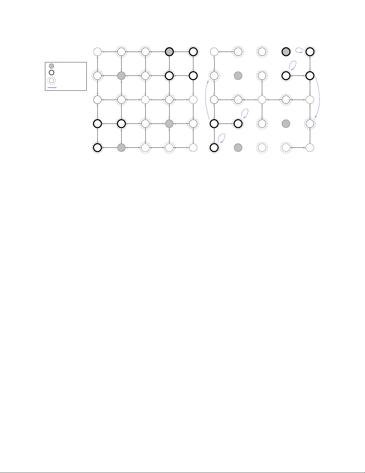
Characteristics of Optimal Solutions to the Sensor Lo cation Problem Da vid. R. Morrison Univ ersit y of Illinois at Urbana-Champaign Champaign, IL Susan. E. Martonosi Harv ey Mudd College 301 Platt Blvd. Claremon t, CA 91711 (909) 607-0481 martonosi@hmc.edu Submitted for publication on Octob er 3, 2010 Abstract: In Bianco et al. (2001), the authors present the Sensor Lo cation Problem: that of lo cating the minim um n um b er of traffic sensors at in tersections of a road net w ork suc h that the traffic flo w on the en tire net w ork can be determined. They offer a necessary and sufficient condition on the set of monitored no des in order for the flow everywhere to b e determined. In this pap er, w e present a counterexample that demonstrates that the condition is not actually sufficient (though it is still necessary). W e present a stronger necessary condition for flow calculabilit y , and show that it is a sufficient condition in a large class of graphs in which a particular subgraph is a tree. Many t ypical road net w orks are included in this category , and we sho w ho w our condition can b e used to inform traffic sensor placement. 1 1 In tro duction T raffic congestion is a significan t problem in most ma jor cities in the world. An imp ortant first step in mitigating road congestion is to kno w the distribution of cars on eac h road of the net w ork. This can b e ac hiev ed by using traffic sensors to count cars trav eling in to and out of an in tersection. Ho w ev er, placing sensors on every in tersection is not only prohibitively expensive, it is also inefficient: if some sensors were remo v ed, traffic flow through those intersections might still b e calculated by applying flo w conserv ation laws and kno wledge of the fraction of cars turning in eac h direction at eac h intersection. In fact, even a v ertex co v er is inefficient for these reasons. Thus, we wan t to lo cate the minimum num ber of sensors such that we can still determine the distribution of cars in the entire net w ork. This problem w as introduced in Bianco et al. (2001) and named the Sensor Lo cation Problem, (SLP). Bianco et al. (2001) present a necessary and sufficient condition on the set M of monitored intersections suc h that the traffic flow on the entire net w ork is calculable. W e present a counterexample demonstrating that the condition, while necessary , is not sufficient. Using the insigh ts pro vided by the coun terexample, w e dev elop a stronger necessary condition that, while not sufficient in general, is sufficient in a large class of net w orks in which a particular unmonitor e d sub gr aph , to be defined in this paper, is a tree. W e presen t sev eral examples of road net w orks, including the standard grid net w ork, to whic h this sufficien t condition can b e used to confirm that the flo w can b e completely specified. Moreov er w e present examples for which the condition is not sufficient, but where the failure of the necessary condition also pro vides useful information ab out the netw ork. First, w e review the terminology and notation used in Bianco et al. (2001). Then, w e present our coun terexample in Section 3, and develop a matrix representation for the problem in Section 4. Section 5 deriv es a graph-theoretic necessary condition for flow calculability , and Section 6 demonstrates that this condition is sufficien t in the case when eac h unmonitored subgraph is a tree. In Section 7 w e pro vide examples of how this new condition could b e used for decision supp ort by traffic engineers. W e offer concluding remarks in Section 8. 2 Definitions Let the road net work b e represen ted b y a directed graph G = ( V , A ), where V is a set of intersections and A is a set of “tw o-w a y” directed arcs (roads). That is, if u, v ∈ V and uv ∈ A , then v u ∈ A , but the traffic flo w on arc uv need not equal that on arc vu . W e represen t the traffic flowing ov er the roads by a net work 2 flo w function f : A → R that satisfies the flow conserv ation law at each vertex v ∈ V : X e ∈ v − f e − X e ∈ v + f e + S v = 0 , (1) where v − is the set of arcs with head at v , v + is the set of arcs with tail at v , and S v is the balancing flow at v ertex v . The sources and sinks of traffic, called cen troids , are the vertices with non-zero balancing flo ws; the set of all such centroids we denote B . Because flow is conserved at each vertex, we hav e P v ∈ V S v = 0. W e assume that while the set B is known, the v alues of the balancing flows for vertices in B are unknown. T o determine the net w ork flo w function f , sensors are placed at v arious in tersections in the road net work. W e denote the set of monitored v ertices b y M . If an in tersection is monitored, then the n umber of cars en tering and lea ving the intersection along each road connected to the in tersection is rev ealed. W e denote the set of vertices directly adjacent to vertices in M via an arc in A as A ( M ). W e finally assume kno wledge of the turning ratios at every intersection in the net w ork. The turning ratio c v u for arc v u at v ertex v is simply the p ercent of incoming traffic to v that leav es along arc v u . That is, f v u = c v u X e ∈ v − f e . (2) Define the turning factor of arc v u with resp ect to given reference arc vw to b e the ratio of their turning ratios: α v u = c v u c v w . (3) Then we can write the flow f v u of any outgoing arc v u from v in terms of f v w as f v u = α v u f v w . (4) The v alues for the turning ratios can be obtained from historical data about traffic patterns if a v ailable, or can b e determined easily by monitoring existing traffic patterns for a short time. When a set M of v ertices is monitored, the flow on all arcs b etw een v ertices in M and betw een M and A ( M ) are known, as well as the balancing flows at eac h cen troid in M . Applying the turning ratios, we also kno w the flo w on all arcs betw een v ertices in A ( M ). W e call the set of arcs connecting vertices in M and A ( M ), on which the flow can b e computed directly from monitoring M and applying turning ratios, the com bined cutset of M : 3 Definition 2.1 (Bianco et al. (2001)) . The com bined cutset of M , C M , is the set of ar cs in the sub gr aph of G induc e d by M ∪ A ( M ) . As an aside, we can also use the turning ratios to determine outgoing flow from vertices in A ( M ) to v ertices neither in A ( M ) nor M ; these arcs are not part of the combined cutset, but will b e used later. W e are now ready to define the Sensor Lo cation Problem (SLP): Definition 2.2 (Sensor Lo cation Problem, Bianco et al. (2001)) . Given a two-way dir e cte d gr aph G = ( V , A ) , a network flow function f and a set of c entr oids B , what is the smal lest set M of monitor e d vertic es such that know le dge of al l turning r atios, the values of f on inc oming and outgoing ar cs of M and b alancing flows S v on M uniquely determines f and the b alancing flows S v everywher e on G ? W e fo cus on the v erification version of SLP and seek a condition to v erify that a proposed set M uniquely determines f and the balancing flows. 3 A prop osed condition and coun terexample W e see from the definition of the combined cutset of M that these are arcs ov er which the problem of determining the flow has already b een solved directly from monitoring. Th us, we can remo v e C M from the graph, and try to use the remaining flow coming out of A ( M ), turning ratios and flow balance equations to determine the flow everywhere else in the graph. W e therefore define the unmonitored subgraph of G to b e the subgraph G 0 that remains when C M has b een remo v ed from the graph: G 0 = ( V − M , A − C M ). This subgraph contains all arcs ov er which the flow is not completely determined by monitoring. The unmonitored subgraph is often, but not alwa ys, disconnected. W e call the i th connected comp onen t of the unmonitored subgraph the i th unmonitored comp onen t and lab el it G 0 i . W e lab el the set of cen troids in that comp onen t B i , and the set of (originally) adjacent vertices in that comp onen t A i ( M ). Bianco et al. (2001) present a pro of of the following condition on the set M in order for the flow function f to b e uniquely determined. While this is a necessary condition, we present an example that demonstrates it is not actually sufficient in general. Theorem 3.1 (Bianco et al. (2001)) . Given a set of monitor e d vertic es M , the flow on a digr aph G c an b e uniquely determine d everywher e if and only if for every unmonitor e d c omp onent G i of G , | B i | ≤ | A i ( M ) | . 4 In their pro of of this theorem, the authors compare the num ber of unknown arc and balancing flow v ariables to the num ber of flow balance and turning ratio equations when this condition holds. They argue (correctly) that the n um b er of equations m ust b e at least the n umber of unkno wns, whic h happ ens only if | B i | ≤ | A i ( M ) | . How ever, in their argument that the condition is sufficient, they neglect the p ossibilit y that some of the resulting equations might b e linearly dep enden t, and thus the solution will not b e unique. T o see this, consider the follo wing example (shown in Figure 1). Let δ + ( u ) be the outgoing degree of v ertex u , and supp ose that the turning ratios c uv = 1 /δ + ( u ) for all arcs uv (the flows on all outgoing arcs from v ertex u are equal). By monitoring v ertex a , the unmonitored subgraph G 0 induced b y removing the com bined cutset has only a single connected comp onen t, consisting of the v ertices b, c, d, e, f and the arcs b et ween them. A ( M ) in this component is { b, d } , and B − M = { e, f } . Thus | A ( M ) | = | B − M | = 2, and b y T heorem 3.1, we should b e able to determine f and the vector S of balancing flows uniquely . Monitored Vertex Centroid Vertex Adjacent Vertex S = ? e S = ? f 4 4 4 4 4 4 4 4 4 4 ? ? a c d b e f Figure 1: A counterexample to the flow calculation theorem (Theorem 3.1). If w e monitor vertex a in the ab o v e graph, the graph with cutset C M = { ab, ba, ad, da } remov ed satisfies the conditions in Theorem 3.1. Howev er, we cannot calculate f ed or f f d from the known information. Ho w ev er, supp ose we observe 4 units of flow along arcs ab, ba, ad, and da . W e apply the flow balance equation and knowledge of the turning ratios sequen tially at each vertex until we get stuck. Consider vertex b . It is not a cen troid, so S b = 0, and since flows on all outgoing arcs are equal, f bc = f ba = 4. T o preserve balance of flo w, f cb = 4 as w ell. By a similar logic, we obtain f cd = f dc = 4 at v ertex c and f de = f d f = 4 at v ertex d . W e cannot determine f ed and f f d b ecause b oth e and f are cen troids, and their balancing flo ws 5 are unknown. Balancing flows in the netw ork must sum to zero, so S f = − S e , leaving us with the following system of equations having three unknowns and three equations, as predicted by Theorem 3.1. f ed + f f d = 8 f ed − S e = 4 f f d + S e = 4 (5) Notice, how ever, that these equations are linearly dep endent and th us fail to admit a unique solution. Therefore, the condition provided in Theorem 3.1 is not sufficient. Unfortunately , there are many suc h coun terexamples, including cases when the graph is a tree or when the inequality in the theorem is strict. F ortunately , the subsequent work of Bianco et al. (2001) and Bianco et al. (2006) is correct despite the erroneous Theorem 3.1. Nonetheless, it is still v aluable to understand why the theorem is incorrect and to formulate a new theorem that guarantees the calculability of traffic flows on a monitored graph. T o better understand the circumstances under whic h Theorem 3.1 fails, we next examine the problem via the graph’s incidence matrix. 4 SLP and Inv ertible Matrices Let E b e the | V | × | A | incidence matrix where the ( u, e ) th en try is − 1 if v ertex u is the tail of arc e , 1 if it is e ’s head, and 0 if e is not incident to u . Let f b e the | A | -length vector of unknown arc flo ws and S the | V | -length vector of balancing flows. The system of linear flow conserv ation constraints at each vertex then tak es the form E f + S = x , (6) where x = 0 . Notice that the sum of these equations yields the balancing flow constraint P u ∈ V S u = 0, so w e do not need to add this constraint to system (6). This system does not include the known turning ratios or the observ ed flo w along monitored arcs, and th us contains more unknown v ariables than are necessary . W e can therefore reduce this system of equations to a more compact representation, as follows: 1. F or each vertex u ∈ V , we designate an arbitrary outgoing arc e u to b e the canonical arc for vertex u . Since we kno w the turning ratios of the graph, the flow ov er an y arc uv is f uv = α uv f e u . This reduces the num b er of flow v ariables from | A | to | V | , and we can mo dify the unkno wn flow vector f to 6 include only the | V | canonical arcs. 2. Having expressed the flo w on any arc uv in terms of the flow on e u , the flow balance matrix E collapses in to a square matrix ˆ E , where ro w u still corresp onds to the balance equation at vertex u , and column v corresponds to the canonical arc for vertex v , e v . The ( u, v ) th en try of ˆ E is given by ˆ E u,v =            α v u if u and v are connected − P w adjacent to u α uw if u = v 0 if u and v are not connected 3. W e also augment ˆ E with | B | columns for the unknown balancing flows at the centroids. The column corresp onding to the cen troid at v ertex u has a 1 in the u th ro w and 0’s everywhere else. Lik ewise, w e create a single ( | V | + | B | )-length vector g =    f S    of unknown canonical arc and balancing flows. Equation (6) then b ecomes ˆ Eg = x , (7) where x is still the zero vector. W e next incorp orate the known flow v alues obtained by monitoring vertices in M . 4. F or eac h v ertex m ∈ M , the flow along m ’s c anonical arc and the balancing flow (if m is a centroid) are kno wn. W e can remov e row m from the matrix ˆ E . W e also remov e column m , corresp onding to v ertex m ’s canonical arc. Next, we up date the right-hand side vector x with the known flow v alues by subtracting f e m times the remov ed m th column from x . This is equiv alent to subracting α mu f e m from the u th en try of x for each vertex u adjacent to m . If m is a centroid, w e also remov e the column of ˆ E corresp onding to its balancing flow. W e lik ewise remov e the entry from g corresponding to f e m (and S m if m is a centroid), and remov e the m th en try from x . 5. F or each v ertex a ∈ A ( M ), the outgoing flow from a to an y vertex m ∈ M is monitored, so b y turning ratios, w e can deduce the flow ov er a ’s canonical arc. W e therefore remov e column a from ˆ E and subtract f e a = 1 α am f am times column a from the right-hand side vector x . This is equiv alen t to subtracting α au f e a from the u th en try of x for eac h vertex u adjacent to a and adding P w adjacent to a α aw f e a to the a th en try of x . W e remo v e the en try from g corresp onding to f e a . 7 S = ? d S = ? f S = ? b f b a c d S = −5 e out = 4 in = 9 e 1 3 2 4 1 2 Adjacent Vertex Centroid Vertex Monitored Vertex Figure 2: A netw ork in which the set of centroids is B = { b, d, e, f } , and vertex e is monitored, revealing the flows indicated on the arcs into and out of e . In this case, we can calculate the flow everywhere on the graph, as demonstrated b y equation (9) having a unique solution. W e name the resulting co efficien t matrix for the system of equations the flo w calculation matrix F and rewrite for the last time our original system of equations Fg = x . (8) If equation (8) has a unique solution (whic h occurs when the columns of F are linearly indep endent), then we can uniquely determine the flow everywhere on the graph. F or example, consider the graph in Figure 2, with M = { e } and flows on monitored arcs as indicated in the figure. W e choose arcs ab, ba, ca, db, ed and f b to b e our canonical representativ es for each v ertex. W e also assume that all turning ratios are equal except at vertex e (so α uv = 1 for all uv 6 = e ), where monitoring has revealed the turning factors to b e α ef = 2 and α ec = 1. The corresp onding reduced system of equations is: 8            − 2 1 0 0 0 1 − 3 1 0 0 1 0 0 0 0 0 1 0 1 0 0 1 0 0 1                       f ab f ba S b S d S f            =            − 3 − 6 5 1 8            (9) It is easy to c hec k that rank( F ) = 5, and th us the columns are linearly indep enden t; this implies that equation (8) is solv able for the graph in Figure 2. 5 A new necessary condition The flow is uniquely calculable if and only if the matrix F has full column rank. An obvious necessary (but insufficien t) condition is for F to ha ve at least as man y rows as columns. F has | V | − | M | − | A ( M ) | + | B − M | columns and | V | − | M | rows. Therefore, w e require | B − M | ≤ | A ( M ) | . The necessary condition prov ed in Bianco et al. (2001) is stronger: | ( B − M ) i | ≤ | A ( M ) i | for all connected comp onents i in the unmonitored subgraph induced by removing the arcs in the combined cutset. In fact, we can pro v e an even stronger necessary condition that relies solely on the top ology of the graph. This condition correctly identifies that the example of Figure 1 will not yield a unique solution, whereas the original condition | ( B − M ) i | ≤ | A ( M ) i | could not predict this. Our difficulty in calculating the flow arose when we reac hed vertex d . Although we knew the flow exiting v ertex d along the arcs tow ard e and f , we were unable to determine the flow entering d b ecause b oth e and f were centroids, contributing unkno wn balancing flows. T raffic originating or terminating at vertices e and f got “mixed up” at vertex d and could not b e uniquely differentiated. This observ ation leads us to define a B -path, which we use to correct Theorem 3.1. Definition 5.1. A B-path is a p ath starting at a c entr oid and ending at a vertex in A ( M ) . This is a similar, but less restrictiv e, definition than that giv en for MB-feasible paths in Bianco et al. (2006). Using this definition, w e presen t the follo wing theorem, which pro vides a stronger necessary condition for flo w calculabilit y . Theorem 5.2 (Statemen t A) . L et G = ( V , A ) b e a two-way dir e cte d gr aph with c entr oid set B , and let M b e a set of monitor e d vertic es. The flow on ar cs in G and the b alancing flow at the vertic es in B c an b e uniquely determine d everywher e only if ther e exists a set P of | B − M | vertex disjoint B -p aths. 9 Monitored Vertex Centroid Vertex Adjacent Vertex B−path b c d f e a b c d f e Figure 3: The graph from Figure 1), together with a set of B -paths. How ever, any two B -paths m ust pass through vertex d , so there is no set of | B − M | disjoint B -paths asso ciated with M . This is a stronger necessary condition than that giv en in Theorem 3.1 b ecause it is not satisfied by our coun terexample in Figure 1. W e see in Figure 3 that an y set of t wo B -paths will be forced to intersect at v ertex d . Thus, the num ber of disjoin t B -paths is smaller than | B − M | and we are unable to calculate the flo w. T o pro v e Theorem 5.2, w e m ust translate its statement related to the topological structure of the net w ork in to our algebraic framework describ ed earlier. W e note first that the num b er of vertex-disjoin t B -paths cannot b e larger than the size of a minim um disconnecting set C b et ween B − M and A ( M ), b y Menger’s theorem. Thus, we require | C | ≥ | B − M | . (In fact, the size of the minimum disconnecting set will never strictly exceed | B − M | ). Next, we partition the graph G into its unmonitored comp onents by remo ving the combined cutset. If u and v are in different partitions in the graph, then there was no path from u to v in G except through M or along an a 1 a 2 edge for some a 1 and a 2 ∈ A ( M ). Because all rows and columns corresponding to M and all columns corresp onding to A ( M ) ha v e b een remov ed from the matrix, vertex u ’s flo w balance equation will not include any e v or S v terms, and e u and S u will not app ear in vertex v ’s flow balance equation. Thus, we can rearrange the flo w calculation matrix F into blo ck form b y collecting ro ws and columns corresponding to vertices in each unmonitored component, and pro ve the theorem for each comp onen t independently . W e 10 rephrase our original theorem accordingly: Theorem 5.2 (Statement B) . L et G, B , and M b e as in The or em 5.2 (Statement A), with the gr aph p artitione d into unmonitor e d c omp onents and the flow c alculation matrix p artitione d into blo cks as describ e d. F or e ach unmonitor e d c omp onent i , let C i b e the minimum vertex cut b etwe en ( B − M ) i and A ( M ) i . (If ( B − M ) i is empty, then let C = ∅ ). rank( F i ) = # { c olumns of F i } (and henc e the flow on G 0 i is c alculable) only if | C i | = | ( B − M ) i | . Pr o of. F or ease of notation, we drop the subscript i and henceforth refer to all sets in the context of a given unmonitored comp onen t i . W e assume the comp onen t contains at least one centroid, otherwise the theorem is true trivially because both B − M and C are empt y . Within component i , w e call V M the set of v ertices that are not in M or A ( M ) and are connected to M b y some path that do es not pass through C (i.e. they are on the M side of the c ut C ). Similarly , we call V B the set of vertices not in B − M that are on the B − M side of the cut. Note that C, A ( M ) , and B − M could all o v erlap, as sho wn in Figure 4; we lab el these intersections as sho wn, where X A ( M ) ,C = ( A ( M ) ∩ C ) \ ( B − M ), X A ( M ) = A ( M ) \ ( C ∪ ( B − M )), etc. Note that since C is b y definition a v ertex cut b et w een B − M and A ( M ), the set X A ( M ) ,B − M = ( A ( M ) ∩ ( B − M )) \ C is empt y . V B X A(M),C X B−M X C,B−M X A(M),C,B−M X C M X A(M) V M B − M C A(M) Figure 4: The partition of the vertex set for Theorem 5.2. V M is the set of unaccounted-for vertices on the M side of the cut, and V B is the set of unaccounted-for vertices on the B − M side of the cut. Bold arro ws indicate p ossible connections b etw een sets. Some of these sets may be empty—in particular, note that by definition, there can b e no vertices in (( B − M ) ∩ A ( M )) \ C , since C must separate B − M and A ( M ). The shaded-in regions corresp ond to the columns included in the submatrix F ∗ . Let us consider a submatrix F ∗ of F that contains only the columns corresp onding to canonical arcs for v ertices in X B − M and V B and to balancing flows at v ertices in X B − M , X C,B − M and X A ( M ) ,C,B − M . These 11 are the shaded regions of Figure 4. Since F has linearly indep enden t columns, F ∗ has full column rank, and K ≤ R − Z , (10) where K is the num b er of columns of F ∗ , R the num b er of rows and Z the num ber of zero ro ws. By construction, K = | X B − M | + | V B | + | B − M | and R = | X A ( M ) | + | X A ( M ) ,C | + | X A ( M ) ,C,B − M | + | X B − M | + | X C | + | X C,B − M | + | V M | + | V B | . Next w e determine Z . As w e see in Figure 4, there are no arcs from vertices in V M or X A ( M ) to v ertices in X B − M or V B b y definition of the cut C . Moreov er, v ertices in V M and X A ( M ) are not centroids. Therefore, the rows in F ∗ corresp onding to v ertices in V M or X A ( M ) are all zero, and Z ≥ | V M | + | X A ( M ) | . Applying inequalit y (10) and canceling common terms, w e see that | B − M | ≤ | X C | + | X A ( M ) ,C | + | X C,B − M | + | X A ( M ) ,C,B − M | = | C | . Because | C | can never exceed | B − M | , w e ha v e | C | = | B − M | .  As an example, we w alk through the construction of the F ∗ -matrix for our original counterexample of Figure 1. W e start with the flo w calculation matrix F in the system of equations Fg = x : b :              1 0 0 0 0              c : − 2 0 0 0 0 d : 1 1 1 0 0 e : 0 − 1 0 1 0 f : 0 0 − 1 0 1            f cb f ed f f d S e S f            =            4 − 8 12 − 4 − 4            (11) When we remo v e the cutset asso ciated with monitored vertex a , the minimum v ertex cut b et ween A ( M ) = { b, d } and B − M = { e, f } is C = { d } . | C | 6 = | B − M | , so w e should not b e able to calculate the flo w. W e generate the F ∗ submatrix using the sets X A ( M ) = { b } , V M = { c } , X A ( M ) ,C = { d } , and X B − M = { e, f } : 12 Monitored Vertex Centroid Vertex Adjacent Vertex B−path b e c a d Figure 5: In this graph, monitoring vertex e creates 2 disjoint B -paths, satisfying the conditions of Theorem 5.2. How ev er, the F matrix do es not ha ve linearly indep enden t columns, and thus we cannot calculate the flow on the graph. F ∗ = ed f d S e S f b :              0 0 0 0              c : 0 0 0 0 d : 1 1 0 0 e : − 1 0 1 0 f : 0 − 1 0 1 (12) Notice that the first tw o rows of the matrix are 0, whic h means that the rank of this submatrix can’t b e any higher than 3. This implies that the rank of F cannot equal the num b er of columns, and thus the flow on the graph cannot b e calculated. 6 A sufficien t condition for trees Next we turn to the question of sufficiency . Unfortunately , the condition is not sufficien t for graphs in general, but is sufficien t in the case of netw orks whose unmonitored comp onen ts are all trees. Figure 5 pro vides an example of a general graph in whic h there are | B − M | vertex-disjoin t B -paths, but the matrix E M still do es not ha v e linearly indep enden t columns and the flow on the graph cannot b e calculated. W e see that the unmonitored subgraph of this example, whic h we obtain by removing M ’s combined cutset (in this case, the arcs ce, ec, de, and ed ), is not a tree. How ever, the follo wing theorem states that as long as the unmonitored 13 comp onen ts of a graph are all trees, our condition is sufficient to guarantee the calculability of traffic flo w. Theorem 6.1. L et G, B , and M b e as in The or em 5.2, with the flow c alculation matrix p artitione d into blo cks as describ e d. F or e ach unmonitor e d c omp onent i , let C i b e the minimum vertex cut b etwe en ( B − M ) i and A ( M ) i . If the i th c omp onent is a tr e e, then rank( F i ) = # { c olumns of F i } (that is, the flow on blo ck i is c alculable) if and only if | C i | = | ( B − M ) i | . Prior to proving this theorem, we first prov e the following lemma: Lemma 6.2. L et G b e a two-way dir e cte d tr e e with known turning r atios, c ontaining no c entr oids and having r o ot vertex r . Supp ose that G is attache d at r to a gr aph ˆ G at vertex v with known flow value f v r . Then f rv = f v r and the flow on G c an b e determine d. Pr o of. W e prov e this by induction on the n um b er n of vertices in G . As a base case, supp ose n = 1, then G con tains only the leaf no de r . Because r is not a cen troid, its balancing flo w is zero, so f rv = f v r , and the flo w on G has b een determined. Supp ose the statement is true for an y tree of size strictly less than n and let G hav e size n . Consider the v ertex r ∈ G which is attac hed to graph ˆ G at v ertex v . Because G is a tree with no cen troids, flow is conserv ed, so f rv = f v r , and all other outgoing flo ws of r can be determined using turning ratios. Moreov er, r is connected to deg( r ) subtrees of G each of size strictly less than n and ha ving ro ot v ertices v i , i = 1 ... deg( r ) with known incoming flow v alues f rv i . So the flow on eac h subtree can also b e determined, and f v i r = f rv i . W e hav e therefore found the flow on the en tire graph.  Th us, on a subtree with no centroids, the flow can be computed kno wing only a single incoming arc to the tree. W e now pro v e Theorem 6.1. Pr o of. Theorem 5.2 handles the necessary condition. Let n = | ( B − M ) i | . Because | C i | = | ( B − M ) i | , | A ( M ) i | m ust also be at least n , and there exists a pairing b etw een a subset of A ( M ) i and the v ertices in ( B − M ) i suc h that the set of paths b etw een all pairs a i ∈ A ( M ) i and b i ∈ ( B − M ) i are vertex disjoint. (If | A ( M ) i | > n , then the “extra” vertices in A ( M ) i will act like centroids with known balancing flo w equal to the incoming flow from M and can b e treated like any other non-cen troid.) W e will induct on n to show ho w to propagate the flow calculation through the graph. If n = 0, then our partition consists of a tree having no centroids that, in the original graph, is connected to a vertex in M . The flow along an incoming arc to G 0 i from M is known due to monitoring, so our Lemma 6.2 tells us that the flow along every arc in G 0 i can b e determined. 14 1 deg(a ) a 1 deg(a ) T 2 1 deg(a ) T T 1 a b m a b a b 1 1 i i 2 2 b w Figure 6: The tree structure induced by the pairing of centroids and adjacent vertices in Theorem 6.1. Note that no path from a vertex a j ∈ A ( M ) to its pair b j ∈ B − M can cross any other vertex in A ( M ). This allows us to treat each subtree separately when calculating the flow along it. Supp ose the theorem is true for an y partition ha ving | ( B − M ) i | < n unmonitored centroids, and consider a partition having | ( B − M ) i | = n . Without loss of generality , consider centroid b 1 and its matching adjacen t v ertex a 1 . Let T 1 , ..., T deg ( a 1 ) b e the subtrees of T ro oted at a 1 ’s neigh b ors t 1 , ..., t deg ( a 1 ) , and assume that T 1 ∪ { a 1 } is the tree containing the ( a 1 , b 1 ) pair (See Figure 6). Ev ery subtree maintains the original pairing of vertices in A ( M ) i and ( B − M ) i b ecause these pairings corresp onded to vertex-disjoin t paths which could not pass through a 1 . Moreo v er, eac h subtree T j , j 6 = 1 has strictly fewer than n such pairings and satisfies the induction h yp othesis. The flow on these subtrees can b e calculated. It remains to determine the flow on the edges b et ween a 1 and t j : f a 1 t j is an outgoing flow from a 1 whic h is known b y monitoring and application of turning ratios. f t j a 1 can b e expressed in terms of the flow on t j ’s canonical edge. Thus, there is still a unique solution for the flo w on T j ∪ { a 1 } , and all incoming flow to a 1 from trees T 2 , ..., T deg ( a 1 ) has been determined. Next we consider the tree T 1 ∪ { a 1 } , by propagating flow calculations along the path from a 1 to b 1 . The outgoing flo w from a 1 along the path is kno wn b y applying turning ratios. If a 1 = b 1 , then in fact T 1 is empt y . a 1 ’s incoming and outgoing flows can b e use d to find its balancing flo w, and the flow on G 0 i has b een completely determined. If a 1 6 = b 1 , the incoming edge to a 1 from the next v ertex on the path to b 1 is the only edge incident to a 1 whose flow has not yet b een determined; it can b e determined by flow conserv ation. By 15 a similar logic, we can propagate these flow calculations along the path from a 1 to b 1 un til we reach the first v ertex w ha ving degree greater than 2. All outgoing flo ws of w are known b y applying turning ratios to the kno wn outgoing flow from w to the vertex preceding w in the path. Each branch of w that do es not contain b 1 is once again a subtree that maintains the (strictly fewer than n ) original ( B − M ) i and A ( M ) i pairings. By our induction hypothesis, the flo w on this branch can be determined and b y the same reasoning as ab ov e, the flow on the edges b etw een w and the branch can also b e determined. Flow conserv ation determines the incoming flow to w from the next vertex on the path to b 1 . W e contin ue this wa y until v ertex b 1 is reached. All outgoing flows from b 1 are determined by applying turning ratios to the kno wn outgoing flow from b 1 in to the vertex preceding b 1 in the path. The flow on branches stemming from b 1 can b e determined by our induction h yp othesis, and the balancing flo w at b 1 is simply the difference betw een all outgoing and incoming flo ws at b 1 . The flo w on the tree has b een calculated.  An obvious corollary is the following: Corollary 6.3. If G is a two-way dir e cte d tr e e with c entr oid set B and monitor e d vertex set M , the flow on G c an b e c alculate d if and only if ther e exist at le ast | B − M | vertex-disjoint p aths b etwe en A ( M ) and B − M . This suggests that it is the presence of cycles in unmonitored subgraphs that can occasionally lead to difficulties in uniquely determining the flow. 7 Applications to traffic sensor placemen t While it might at first seem restrictiv e to require the unmonitored subgraph to be a tree in order to guarantee flo w calculabilit y , we sho w in this section that this is not the case. In fact, a broad collection of road netw orks can hav e trees as unmonitored subgraphs. Moreo v er, even for those netw orks whose unmonitored subgraphs con tain cycles, our condition can still provide useful information ab out the placemen t of traffic sensors. Consider the traffic netw ork shown in Figure 7(a). This is a traditional grid net w ork found in many cities, and it has tw ent y-five intersections, of which seven are considered to b e cen troids. A traffic planner migh t b e interested in monitoring four in tersections on the netw ork to calculate the traffic flow throughout it. If she places the monitors on the four v ertices shaded in Figure 7(a), then the unmonitored subgraph is as sho wn in Figure 7(b). The condition of Theorem 3.1 that | B − M | i ≤ | A ( M ) i | is satisfied on both unmonitored comp onen ts, but the rightmost comp onen t violates our necessary condition of Theorem 5.2 16 Monitored Vertex Centroid Vertex Adjacent Vertex B−path (a) Original road netw ork X (b) Unmonitored subgraph obtained by removing the combined cutset C M Figure 7: A road net w ork with four monitored v ertices (shaded) and seven centroid v ertices (bold). The unmonitored subgraph has tw o comp onen ts. The leftmost component has three cen troids and five vertices in A ( M ), satisfying the necessary condition of Theorem 3.1. All centroids hav e a corresp onding B-path, but b ecause this unmonitored comp onen t is not a tree, we cannot be certain that the flow is calculable on this region of the net w ork. The rightmost comp onen t has four cen troids and fiv e vertices in A ( M ), satisfying the necessary condition of Theorem 3.1. Ho w ev er, the centroid lab eled X do es not hav e its own B-path in this unmonitored comp onen t, and hence the traffic flo w is not calculable in this region of the netw ork, by Theorem 5.2 (Statement A). (Statemen t A) because the centroid mark ed by X do es not ha ve its o wn B-path. Therefore, we are able to conclude that flo w is not calculable in this region of the netw ork. The leftmost unmonitored comp onent satisfies our necessary condition, but because this comp onent is not a tree, we are unable to conclude that the flow is calculable in this region. If the traffic planner simply rearranges tw o of the monitored vertices, as shown in Figure 8, she is easily able to construct a netw ork whose unmonitored subgraph is a tree. The sufficient condition of Theorem 6.1 is satisfied, and she can conclude that by placing the monitors in this orientation, the traffic flow on the net w ork will b e completely calculable. It is worth p ointing out that unmonitored subgraphs migh t b e trees even on v ery large graphs with only a small fraction of monitored vertices. W e considered an 18 × 18 grid net w ork (324 vertices) on which 72 v ertices were monitored and all unmonitored subgraphs were trees satisfying the sufficient condition for flo w calculabilit y given by Theorem 6.1. More generally , it could b e expanded to a 3 k × 3 k graph for any integer k having 12 k monitored vertices. Many more examples of large traffic net w orks can b e found for whic h Theorem 6.1 applies. And as we hav e seen in Figure 7, even when the unmonitored subgraph is not a tree, 17 Monitored Vertex Centroid Vertex Adjacent Vertex B−path (a) Original road netw ork (b) Unmonitored subgraph obtained by removing the combined cutset C M Figure 8: A road net w ork with four monitored v ertices (shaded) and seven centroid v ertices (bold). This net w ork is identical to that of Figure 7 except that t w o of the monitored vertices hav e changed p osition. In this mo dified graph, the unmonitored subgraph is a tree, and every centroid has its o wn B-path. Thus, Theorem 6.1 guarantees the traffic flow is fully calculable on this netw ork. failure to satisfy the necessary condition of Theorem 5.2 signals the need either to increase the num b er of sensors, or to rearrange their p ositions until the flow is calculable. 8 Conclusions W e ha v e corrected an error in an earlier theorem regarding when a prop osed set of vertices M in a tw o- w a y directed graph is a v alid monitoring set for determining the flo w on the en tire graph. The top ological insigh ts of our counterexample led us to pro v e a new, stronger, necessary condition that is also sufficient on an y unmonitored subgraph of the net work that is a tree. W e then sho w ed b y example the broad arra y of netw orks in which this condition could be used by traffic engineers to determine the placement of traffic sensors. References Bianco, Lucio, Giusepp e Confessore, and Monica Gen tili. 2006. Com binatorial asp ects of the sensor lo cation problem. A nnals of Op er ations R ese ar ch 144(1):201–234. 18 Bianco, Lucio, Giusepp e Confessore, and Pierfrancesco Rev erb eri. 2001. A net w ork based mo del for traffic sensor lo cation with implications on O/D matrix estimates. T r ansp ortation Scienc e 35(1):50–60. 19