Incentive-aware Contextual Pricing with Non-parametric Market Noise

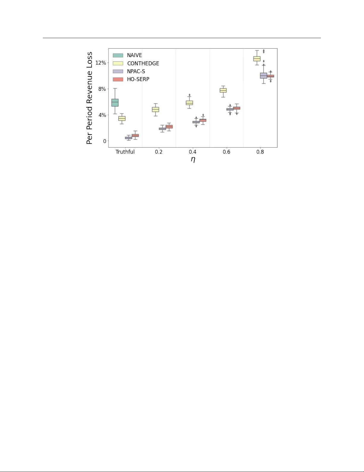
Incen tiv e-a w are Con textual Pricing with Non-parametric Mark et Noise Negin Golrezaei Sloan School of Management, Massac husetts Institute of T echnology , golrezae@mit.edu P atrick Jaillet Department of Electrical Engineering and Computer Science, Massac husetts Institute of T echnology , jaillet@mit.edu Jason Cheuk Nam Liang Operations Research Center, Massac husetts Institute of T echnology , jcnliang@mit.edu W e consider a dynamic pricing problem for repeated contextual second-price auctions with m ultiple strategic buy ers who aim to maximize their long-term time discoun ted utility . The seller has limited information on buy ers’ ov erall demand curves whic h dep ends on a non-parametric market-noise distribution, and buyers ma y p oten tially submit corrupted bids (relative to true v aluations) to manipulate the seller’s pricing p olicy for more fav orable reserve prices in the future. W e fo cus on designing the seller’s learning p olicy to set contextual reserv e prices where the seller’s goal is to minimize regret compared to the reven ue of a b enc hmark clairvo yan t p olicy that has full information of buy ers’ demand. W e prop ose a p olicy with a phased-structure that incorp orates randomized “isolation" p eriods, during which a buyer is randomly c hosen to solely participate in the auction. W e show that this design allo ws the seller to control the num b er of perio ds in which buyers significan tly corrupt their bids. W e then prov e that our p olicy enjoys a T -p eriod regret of e O ( √ T ) facing strategic buyers. Finally , w e conduct numerical simulations to compare our prop osed algorithm to standard pricing p olicies. Our numerical results show that our algorithm outp erforms these p olicies under v arious buy er bidding b eha vior. Key wor ds : online advertising, pricing, online learning, mechanism design,strategic agents 1. In tro duction W e study the problem of designing pricing p olicies for highly heterogeneous items against strategic agen ts. The motiv ation comes from the av ailability of massive amount of real-time data in online platforms and in particular, online adv ertising markets, where the seller has access to detailed information ab out item features/contexts. In suc h environmen ts, designing optimal p olicies inv olv es learning buy ers’ demand (which is a mapping from item features and offered prices to the likelihoo d of the item b eing sold) under limited understanding of buyers’ behavior. Our k ey goal is to dev elop effectiv e and robust dynamic pricing p olices that facilitate such a complex learning pro cess for very general non-parametric con textual demand curves facing strategic buy ers. F ormally , w e study the setting wherein an y p erio d t o ver a finite time horizon T , the seller sells one item to buyers via running a second price auction with a reserv e price. The item is characterized b y a d -dimensional con text vector x t , public to the seller and buyers. W e consider an in terdep endent con textual v aluation mo del in whic h a buy er’s v aluation for the item is the sum of common and 1 2 priv ate components. The common component determines the expected willingness-to-pa y of buyers and is the inner pro duct of the feature vector and a fixed “mean v ector" β that is homogeneous across buy ers; the priv ate comp onen t, which captures buyers’ idiosyncratic preferences, is indep enden tly sampled from an unknown non-p ar ametric noise distribution F . W e note that such a linear v aluation mo del is v ery common in the literature of dynamic pricing; e.g. see Golrezaei et al. (2018), Ja v anmard and Nazerzadeh (2016), Kanoria and Nazerzadeh (2017) and Ja v anmard (2017). Under this in terdep enden t contextual v aluation mo del, we study a str ate gic setting where buy ers in tend to maximize long-term discoun ted utilit y and ma y consequently submit c orrupte d , i.e., un truthful, bids. The motiv ation of this strategic setting comes from the rep eated buyer-seller in teractions when the seller do es not p ossess full information on buy ers’ demand and aims to learn it using buy ers’ submitted bids. In a single-shot second price auction, where there is no rep eated in teractions b etw een the seller and buy ers, bidding truthfully is a buyer’s w eakly dominant action. Ho wev er, this is no longer the case in our rep eated second price auction setting: rep eated auctions ma y incentivize the buy ers to submit corrupted bids, rather than their true v aluations, in order to manipulate seller’s future reserv e prices; e.g. by underbidding, buy ers may trick the seller to lo wer future reserv e prices. In this work, w e would lik e to design a reserve price p olicy for the seller who do es not kno w the mean v ector β and the noise distribution F . The p olicy dynamically learns/optimizes con textual reserve prices while b eing robust to corrupted data (bids), submitted by strategic buy ers. In particular, our ob jective is to minimize our policy’s regret computed against a clairvo yan t b enc hmark p olicy that kno ws b oth β and F . Designing lo w-regret p olicies in our setting in volv es ov ercoming the follo wing c hallenges: (i) The demand curv e is constantly shifting due to the change in contexts ov er time. (ii) The shap e of the demand curve is unkno wn due to the lack of information on the market noise distribution F whic h may not enjo y a parametric functional form. F urthermore, we do not imp ose the Monotone Hazar d R ate (MHR) 1 assumption on F . While the MHR assumption is common in the related literature and can significantly simplify reserv e price optimization (see e.g. Remark 1), it has b een sho wn to fail in practice (see Celis et al. (2014), Golrezaei et al. (2017)). (iii) As stated earlier, in our strategic setting, buy ers may take adv antage of the seller’s lack of knowledge about buy ers’ demand and submit corrupted bids to manipulate future reserv e prices. Main con tribution. W e dev elop a policy called Non-Par ametric Contextual Policy against Str ate gic Buyers (NP A C-S) that enables the seller to efficiently learn the optimal contextual reserv e prices while b eing robust against buyers’ corrupted bids. Our p olicy design incorporates t wo simple y et effective features, namely a phase d structur e and r andom isolation . First, NP AC-S partitions the 1 Distribution F is MHR if f ( z ) 1 − F ( z ) is n on-decreasing in z , where f is the corresponding pdf. 3 en tire horizon in to consecutiv e phases, and then estimates the mean vector and the distributions of the second-highest and highest v aluations only using data from the previous phase. This reduces the buy ers’ manipulating p ow er on future reserve prices as past corrupted bids prior to the previous phase will not affect future pricing decisions. Second, the NP A C-S p olicy incorporates randomized isolation p eriods, that is, in eac h p erio d with some probability the seller chooses a particular buy er at random and let her b e the single participant of the auction during this p erio d. In these isolation p eriods, the isolated buyer faces no comp etition from other buy ers, and hence may incur large utility loss if a significan tly corrupted bid is submitted. 2 F or our main theoretical results, w e show that in virtue of our isolation perio ds in our design of NP A C-S, the n umber of past p erio ds with large corruptions is O ( log ( t )) for any p erio d t via lev eraging the fact that buyers aim to maximize their long-term discounted utility . F urthermore, w e presen t no vel high probabilit y b ounds for our estimation errors in β and F whic h are estimated b y ordinary least squares and empirical distributions, resp ectiv ely , with the presence of corrupted bids. Finally , in Theorem 1, we show that the NP A C-S p olicy ac hieves a regret of ˜ O ( d √ T ) for general non-parametric distributions F against a clairvo yan t b enc hmark p olicy . Related literature. Here w e discuss related works that study dynamic pricing against strategic buy ers with sto chastic v aluations, 3 and refer readers to App endix A for broader related w orks. Both Amin et al. (2013, 2014) study a dynamic pricing problem in a p osted price auction against a single strategic buy er. Amin et al. (2013) addresses the non-contextual sto c hastic v aluation setting, where as Amin et al. (2014) studies a linear con textual v aluation mo del, but with no market noise disturbance. Amin et al. (2014) prop oses an algorithm that achiev es e O ( T 2 / 3 ) regret in con trast with our regret of e O ( √ T ) using the NP A C-S p olicy . W e point out that this is b ecause the seller in their setting only observ es the outcome of the auction (i.e. bandit feedback), while in our setting w e assume that seller can examine all submitted bids. Our setting is more complex compared to Amin et al. (2013, 2014) as w e handle the con textual pricing problem against m ultiple strategic buy ers, and also deals with the issue of learning a non-parametric distribution function in the presence of strategic buyer b eha vior. Kanoria and Nazerzadeh (2017) consider a con textual buy er v aluation mo del similar to ours (but with the MHR assumption on the market noise distribution) and prop oses 2 In the isolation perio ds, when the v aluation of the isolated buyer is greater than the reserv e price, significantly underbidding may cause the item to not be allocated; when the v aluation of the isolated buyer is low er than the reserv e price, o v erbi dding results in the buy er pa ying m uc h higher prices (relative to v aluation) to ac hieve the item. In either case, the isolated buyer will incur a significant utility loss compared to truthful bidding. 3 The general theme of learning in the presence of strategic agents or corrupted information has also been studied in other applications; see, for example, Chen and Keskin (2018), Birge et al. (2018), F eng et al. (2019). There are also related works that study adversarial buyer v aluations. F or example, Drutsa (2019) studies the seller’s pricing problem for rep eated second-price auctions facing m ultiple strategic buyers with priv ate v aluations fixed ov ertime. In addition, buyers in this work also seek to maximize cum ulative discounted utility . The pap er prop oses an algorithm that achiev es O (log log( T )) regret for worst-case (adversarial) v aluations. 4 a pricing algorithm that sets p ersonalized reserv e prices for individual buy ers. They argue that the design of their algorithm induces an equilibrium where buy ers alwa ys bid truthfully , and then further assume buy ers act according to this equilibrium. Our w ork distinguishes itself from t wo asp ects. First, setting p ersonalized reserve prices in Kanoria and Nazerzadeh (2017) rely crucially on the MHR assumption, and in this pap er we relax this assumption such that our metho dology works for a larger class of market noise distributions. Second, w e consider more general buyers who do not necessarily pla y any equilibrium and are forward lo oking. Golrezaei et al. (2018) study a similar in terdep endent con textual v aluation mo del to ours, but with heterogeneous mean v ector β across agent s. Our work distinguishes itself from Golrezaei et al. (2018) in t wo ma jor wa ys. First, they fo cus on optimizing con textual reserv e w.r.t. the w orst-case distribution among a known class of MHR mark et noise distributions. In contrast, our work relaxes this constraint and do es not require the seller to ha ve an y prior kno wledge on the p ossibly non-parametric distribution. Second, in their setting, the seller only utilizes the outcome of the auctions to learn buyer demand and results in a regret of e O ( T 2 / 3 ) . 4 In our w ork, we exploit the information of all submitted bids by taking adv antage of the fact that buy ers’ utility-maximizing behaviour constrains their degree of corruption on bids. This ev entually allo ws us to achiev e an improv ed regret of e O ( √ T ) . Nevertheless, our prop osed algorithm cannot not handle heterogeneous β ’s, and hence this will b e an in teresting future research direction. Drutsa (2020) studies the p osted price selling problem against a strategic agen t with a non-linear (stochastic) con textual v aluation mo del that satisfies some Lipschitz condition with no additive noise. W e summarize some k ey differences in the settings/results of the aforementioned w orks in T able 1. Algorithm # buyers Con text Noise/v alue dist. Discoun t util. Regret Phased Amin et al. (2013) 1 F alse Lipsc hitz T rue Sublinear 5 LEAP Amin et al. (2014) 1 T rue No additive noise T rue O ( T 2 / 3 ) PELS Drutsa (2020) 1 T rue No additive noise T rue O ( T d/ ( d +1) ) HO-SERP Kanoria and Nazerzadeh (2021) ≥ 2 T rue MHR F alse O ( √ T ) SCORP Golrezaei et al. (2018) ≥ 2 T rue MHR T rue O ( T 2 / 3 ) NP AC-S (this w ork) ≥ 2 T rue Non-parametric T rue O ( √ T ) T able 1: Summary of settings and results for seller algorithms that sell against strategic agents with stochastic v aluations. Note that the Discount util. column indicates whether the algorithm deals with buy ers who discount their long-term utilities. Note that HO-SERPKanoria and Nazerzadeh (2021) and SCORP Golrezaei et al. (2018) set p ersonalize d r eserve pric es for each buy er, whereas NP AC-S sets a single reserve for all buyers. PELS in Drutsa (2020) learns a non-linear contextual v aluation model and hence yields larger regret. Among all algorithms, only SCORP Golrezaei et al. (2018) handles heterogeneous β across buyers. 4 A recen t w ork Deng et al. (2019) builds on the result of Golrezaei et al. (2018) b y considering a stronger b enc hmark that kno ws future buyer v aluation distributions (noise distribution and all the future con textual information). They design robust pricing sc hemes whose regret is O ( T 5 / 6 ) against the aforementioned b enc hmark, confirming the generalizabilit y of pri cing schemes in Golrezaei et al. (2018). 5 2. Preliminaries Notation. F or a ∈ N + , denote [ a ] = { 1 , 2 , . . . , a } . F or t w o vectors x, y ∈ R d , denote h x, y i as their inner pro duct. Finally , I {·} is the indicator function: I {A} = 1 if ev ent A o ccurs and 0 otherwise. W e consider a seller who runs rep eated second price auctions o ver a horizon with length T that is unknown to the seller. In each auction t ∈ [ T ] , an item is sold to N buy ers, where the item is c haracterized b y a d -dimensional feature vector x t ∈ X ⊂ { x ∈ R d : k x k ∞ ≤ x max } where 0 < x max < ∞ . W e assume that x t is indep enden tly drawn from some distribution D unkno wn to the seller. W e define Σ as the cov ariance matrix of distribution D . 6 W e assume that Σ is p ositiv e definite and unkno wn to the seller, and define the smallest eigen v alue of Σ to b e λ 0 > 0 . Buy er v aluation mo del. W e fo cus on an in terdep endent v aluation mo del where the v aluation of buy er i ∈ [ N ] at time t ∈ [ T ] is given b y v i,t = h β , x t i +  i,t . Here, β is called the me an ve ctor and is fixed o ver time and unkno wn to the seller, while  i,t is idiosyncratic mark et noise sampled indep enden tly o ver time and across buy ers from some time-inv ariant distribution F with probability density function f , both unknown to the seller. F urthermore, F has bounded supp ort ( −  max ,  max ) , in which its probabilit y density function is b ounded by c f := sup z ∈ [ −  max , max ] f ( z ) ≥ inf z ∈ [ −  max , max ] f ( z ) > 0 . The supp ort b oundary  max is not necessarily kno wn to the seller. W e assume there exist v max > 0 so that v i,t ∈ [0 , v max ] for all i ∈ [ N ] , t ∈ [ T ] . W e highlight that our setting do es not enforce distribution F to be parametric nor to satisfy the MHR assumption. This is b ecause via analyzing real auction data sets, it has b een sho wn that the MHR assumption do es not necessarily hold in online advertising markets Celis et al. (2014), Golrezaei et al. (2017). Rep eated contextual second price auctions with reserv e. The con textual second price auction with reserv e is describ ed as follo wed for N ≥ 2 buyers: In any p erio d t ≥ 1 , a con text v ector x t ∼ D is rev ealed to the seller and buy ers. The seller then computes reserv e price r t , while sim ultaneously each buy er i ∈ [ N ] forms individual v aluations v i,t and submits a bid b i,t to the seller. Let i ? = arg max i ∈ [ N ] b i,t b e the buy er who submitted the highest bid. 7 If b i ? ,t ≥ r t , the item is allo cated to buy er i ? and he is charged the maxim um b et ween the reserv e price and second highest bid, i.e. buy er i ? pa ys p i ? ,t = max { r t , max i 6 = i ? b i,t } . F or an y other buyer i 6 = i ? , the pa yment p i,t = 0 . In the case where b i ? ,t < r t , the item is not allo cated and all pa yments are zero. Here, the seller’s reserv e price r t can only depend on x t and the history set H t − 1 := { ( r 1 , { b i, 1 } i ∈ [ N ] , x 1 ) , . . . , ( r t − 1 , { b i,t − 1 } i ∈ [ N ] , x t − 1 ) } whic h includes all information a v ailable to the seller up to p eriod t − 1 . 6 The co v ariance matrix of a distribution P on R d is defined as E x ∼P [ xx > ] − µµ > , where µ = E x ∼P [ x ] . 7 No ties will occur since w e assume that no v aluations and bids are the same. 6 Buy ers’ bidding b eha vior. In the setting where buyers are strategic, we assume that in an y p eriod t , each buy er i ∈ [ N ] aims at maximizing his long-term discounted utility U i,t : U i,t := T X τ = t η τ E [ v i,τ w i,τ − p i,τ ] , (1) where η ∈ (0 , 1) is the discount factor, w i,t ∈ { 0 , 1 } indicates whether buyer i wins the item, and the exp ectation is tak en with resp ect to the randomness due to the noise distribution F , the con text distribution D , and buyers’ bidding b eha vior. W e p oin t out that this discoun ted utility mo del illustrates the fact that buy ers are less patient than the seller, and is a common framework in man y dynamic pricing literature; see Amin et al. (2013, 2014), Golrezaei et al. (2018), and Liu et al. (2018). The motiv ation lies in many applications in online adv ertisemen t mark ets wherein the user traffic is usually very uncertain and as a result, adv ertisers (buy ers) would not like to miss out an opp ortunity of sho wing their ads to targeted users. It is worth noting that Amin et al. (2013) show ed, in the case of a single buyer, it is not p ossible to obtain a no-regret p olicy when η = 1 , that is, when the buyer is as patien t as the seller. F urthermore, w e assume buyers corrupt their true v aluations in an additive manner: ∀ i ∈ [ N ] , t ∈ [ T ] b i,t = v i,t − a i,t where | a i,t | ≤ a max . Here, a i,t is called the degree of corruption, and we refer to the buy er b ehavior of submitting a bid b i,t 6 = v i,t (i.e., a i,t 6 = 0 ) as “corrupted bidding”. Note that when a i,t > 0 , the buy er shades her bid, and when a i,t < 0 , the buyer o verbids. Essen tially , a buy er i ’s strategic b ehavior is equiv alen t to deciding on a non-zero v alue of a i,t . In this w ork, we imp ose no restrictions on the degree of corruption a i,t for a buy er i in p eriod t other than it is b ounded. 8 3. Benc hmark and Seller’s Regret The seller’s reven ue in p eriod t ∈ [ T ] is the sum of total paymen ts from all buyers, and the exp ected rev enue giv en context x t ∈ X and reserv e price r t is rev t ( r t ) := E h X i ∈ [ N ] p i,t    x t , r t i , where p i,t = max { b − t , r t } I { b i,t ≥ max { b + t , r t }} . (2) Here, b − t and b + t are the second-highest and highest bids in p erio d t , resp ectiv ely; the exp ectation is tak en with respect to the noise distribution in p erio d t and any randomness in the reserve price r t as w ell as bid v alues submitted by buy ers in p erio d t (as buyers’ bidding strategies ma y be randomized). 8 A bound for the degree of corruption is natural as buyers alwa ys submit non negative bids and all bids are b ounded b y v max . 7 The seller’s ob jective is to maximize his expected reven ue ov er a fixed time horizon T through optimizing contextual reserve prices r t for any t ∈ [ T ] . T o ev aluate any seller pricing p olicy , we compare its total reven ue against that of a b enc hmark p olicy run by a clairv oy ant seller who kno ws the mean vector β and the non-parametric noise distribution F . This clairvo yan t seller’s b enchmark p olicy sets the “optimal” con textual reserv e price in eac h p eriod to obtain the maximum achiev able rev enue max r rev t ( r ) in each p eriod, and hence facing such a seller there will be no incen tive for buy ers’ to corrupt their bids. T o provide a more formal definition for the rev en ue of the clairv oy ant seller as w ell as “optimality” in contextual reserve prices, w e rely on the following prop osition that c haracterizes the seller’s conditional exp ected reven ue when buyers bid truthfully . Prop osition 1 (Seller’s Rev enue with T ruthful Buy ers) Consider the c ase of N ≥ 2 buyers who bid their true valuations, i.e., v i,t = b i,t for any i ∈ [ N ] and t ∈ [ T ] . Conditione d on the r eserve pric e r t and the curr ent c ontext x t ∈ X , the sel ler’s single p erio d exp e cte d r evenue in Equation (2) is Z ∞ −∞ z dF − ( z ) + h β , x t i + Z r t 0 F − ( z − h β , x t i ) dz − r t  F + ( r t − h β , x t i )  , (3) wher e for any z ∈ R , F − ( z ) := N F N − 1 ( z ) − ( N − 1) F N ( z ) and F + ( z ) := F N ( z ) . The pro of for this prop osition is detailed in App endix B. In Prop osition 1, F + ( · ) and F − ( · ) are the cum ulative distribution functions of  + t := v + t − h β , x t i and  − t := v − t − h β , x t i resp ectiv ely , where v + t and v − t are the highest and second highest v aluations in p eriod t ∈ [ T ] . In ligh t of Prop osition 1, w e define the b enc hmark p olicy of the clairv oy an t seller as follo w ed, Definition 1 (Benchmark P olicy) The b enchmark p olicy knows the me an ve ctor β and noise distribution F , and sets the r eserve pric e for a c ontext ve ctor x ∈ X as r ? ( x ) = arg max y ≥ 0 Z y 0 F − ( z − h β , x i ) dz − y  F + ( y − h β , x i )  . (4) Ther efor e, the b enchmark r eserve pric e in p erio d t , denote d by r ? t , is r ? ( x t ) , and the c orr esp onding optimal r evenue, denote d by REV ? t , is e qual to Z ∞ −∞ z dF − ( z ) + h β , x t i + Z r ? ( x t ) 0 F − ( z − h β , x t i ) dz − r ? ( x t )  F + ( r ? ( x t ) − h β , x t i )  . Remark 1 When distribution F satisfies the MHR assumption, the obje ctive function of the opti- mization pr oblem in Equation (4) is unimo dal in the de cision variable y , and ac c or ding to Golr ezaei et al. (2018), r ? ( x ) c an b e simplifie d as fol lows: r ? ( x ) = arg max y ≥ 0 y (1 − F ( y − h β , x i )) . In wor ds, the MHR assumption de c ouples the r eserve pric e optimization pr oblem for multiple agents to the much simpler monop olistic pricing for e ach individual agent. 8 W e observ e this b enc hmark provides an optimal mapping from the feature v ector x t to reserv e price r ? ( x t ) , whic h remains unchanged ov er time as the mean vector β and noise distribution F are time-in v ariant. This ec ho es our earlier p oin t that pricing is challenging in our con textual setting since w e w ould need to approximate or learn the optimal mapping r ? ( · ) , whereas in non-contextual en vironments it is sufficien t to learn a single optimal reserve price v alue. W e no w pro ceed to define the regret of a p olicy π (p ossibly random) when the regret is measured against the b enc hmark p olicy . Suppose that in any p erio d t , p olicy π selects reserv e price r π t . Then, the regret of p olicy π in p eriod t and its cum ulative T -p erio d regret are defined as: Regret π ( T ) = X t ∈ [ T ] E [ REV ? t − rev t ( r π t ) ] , (5) where the optimal reven ue REV ? t is giv en in Definition 1, and the exp ectation is taken with resp ect to the con text distribution D as w ell as the p ossible randomness in the actual reserve price r π t . Our goal is to design a p olicy that obtains a lo w regret for any β , F , and con text distribution D . 4. The NP A C-S P olicy In this section, we first prop ose a p olicy called Non-Par ametric Contextual Policy against Str ate gic Buyers (NP A C-S) to maximize seller’s exp ected rev en ue in our strategic setting. Then, we provide insigh ts in to ho w our design in NP AC-S makes the p olicy robust to buyer strategic behavior, and in turn allo ws the p olicy to learn the mean vector β and noise distribution F efficien tly . Finally , we presen t theoretical regret guarantees for NP AC-S against the clairv o yan t b enc hmark described in Definition 1 that sets the optimal con textual reserv e price defined in Equation (4). The NP A C-S p olicy . The detailed NP A C-S p olicy is shown in Algorithm 1, and consists of three main comp onents. (i) Phase d Structur e: NP A C-S partitions T in to consecutiv e phases, where eac h phase ` ≥ 1 , denoted as E ` , has length T 1 − 2 − ` . This implies | E 1 | = √ T and | E ` | / p | E ` − 1 | = √ T . Here, we can establish that the total num b er of phases can b e upper b ounded by d log 2 ( log 2 ( T )) e + 1 . (ii) Estimation for β , F − and F + : A t the end of each phase, NP A C-S uses the submitted bids from the p ervious phase and emplo ys Ordinary Least Squares (OLS) and empirical distributions to estimate the mean v ector β as well as F , resp ectively . (iii) R andom isolation: NP AC-S incorp orates random isolation p erio ds in whic h a single buyer is c hosen at random, and the item is auctioned to this isolated buy er (i.e. the seller only considers the bid of the isolated buy er and ignores bid from other buy ers). 9 Note that when a buy er i is isolated, the buy er wins the item if and only if his bid is greater than the reserve price, and pa ys the reserv e price if he wins. Here, the seller’s pricing p olicy is announced to all buyers (at t = 0 ) so that buy ers examine the p olicy and hav e the freedom to adopt an y bidding strategy to maximize their long term discoun ted utility . 9 The seller discloses her commitment to the random isolation protocol to all buyers at t = 0 , and it is not necessary for the seller to reveal, during an isolation p eriod, which buyer is being isolated. 9 Algorithm 1 Non-Parametric Contextual P olicy against Strategic Buyers (NP AC-S) 1: Initialize b β 1 = 0 , and b F − 1 ( z ) = b F + 1 ( z ) = 0 for ∀ z ∈ R . 2: for phase ` ≥ 1 do 3: for t ∈ E ` do 4: Isolation : With probability 1 / | E ` | , c ho ose one buyer uniformly at random and offer price r u t ∼ Uniform (0 , v max ) . (6) 5: No Isolation : With probability 1 − 1 / | E ` | , set reserve price for all buyers as b r t = arg max y ∈ [0 ,v max ] Z y 0 b F − ` ( z − h b β ` , x t i ) dz − y · b F + ` ( y − h b β ` , x t i ) . (7) 6: Observ e all bids { b i,t } i ∈ [ N ] 7: end for 8: Up date estimate of the mean v ector β : a b β ` +1 = ( X τ ∈ E ` x τ x > τ ) † · ( X τ ∈ E ` x τ ¯ b τ ) , (8) where ¯ b τ = 1 N P i ∈ [ N ] b i,τ . 9: Up date the estimate of F + and F − : b F − ` +1 ( z ) = N b F N − 1 ` +1 ( z ) − ( N − 1) b F N ` +1 ( z ) and b F + ` +1 ( z ) = b F N ` +1 ( z ) . (9) where b F ` +1 ( z ) is defined as b F ` +1 ( z ) = 1 N | E ` | X τ ∈ E ` X i ∈ [ N ] I ( b i,τ − h b β ` +1 , x τ i ≤ z ) , (10) 10: end for Remark 2 Her e, we c omment on how one c an solve the r eserve pric e optimization pr oblem in Equa- tion (7). The key observation is that for any p erio d t , b F ` ( · ) is a step function with jumps at p oints in the finite set C ` := { b i,τ − h b β ` , x τ i} i ∈ [ N ] ,τ ∈ E ` − 1 . This implies that in or der to solve for r t in Equation (7), it suffic es to c onduct a grid se ar ch for ∀ y ∈ C ` . Mor e sp e cific al ly, we let { z (0) , z (1) , . . . z ( M ) } b e the or der e d list (in incr e asing or der) of al l elements in C ` ∪ { 0 } , wher e z (0) := 0 and M := |C ` | (her e, we assume d that 0 / ∈ C ` without loss of gener ality). Henc e, r t is e qual to arg max m ∈ [ M ] m X j =1 b F − ` ( z ( j ) − h b β ` , x t i ) · ( z ( j ) − z ( j − 1) ) − z ( m ) b F + ` ( z ( m ) − h b β ` , x t i ) . This shows that the c omplexity to solve Equation (7) is O ( M 2 ) . Mor e detaile d discussions and efficient algorithms r e gar ding r elate d pr oblems c an b e found in Mohri and Me dina (2016). Motiv ation for design of NP A C-S. Here w e pro vide some insigh ts in to the design of the NP AC-S policy , particularly the phased structure and the incorp oration of random isolation p erio ds. a F or a matrix A , A † represen ts its pseudo in verse, so if A is in vertible, we hav e A † = A − 1 . In Lemma 4 of App endix C, w e sho w that with high probability P τ x τ x > τ is positive definite, and hence inv ertible. 10 Due to the phased structure of the algorithm, our estimates for β , F − , and F + only dep end on the bids and con textual features in the previous phase. Th us, corrupted bids submitted by buyers in past p eriods will hav e no impact on future estimates as well as pricing decisions. One can think of this as erasing all memory prior to the previous phase and restarting the algorithm, which can p oten tially reduce buyers’ manipulating p ow er on our estimates and reserve prices. W e no w discuss the impact of ha ving isolation p erio ds. As all buyers are a ware of the randomized isolation proto col, the presence of isolation p eriods restricts buyers from significan tly corrupting their bids to o often as b y doing so they ma y suffer a substan tial utilit y loss when they are isolated. T o illustrate this p oin t with an example, compare the following scenarios: (i) if there are no isolation p eriods, a buyer having the lo west v aluation among all buyers may submit a bid by adding large corruption, but still ending up not b eing the second highest or highest bidder. Assuming that other buy ers bid truthfully , such a scenario will not lead to any changes in utilit y of any buyer, but in tro duces a large outlier to the set of data p oints used in our estimations. In words, when no isolation occurs, buyers may be able to distort the seller’s learning pro cess without facing unfa vorable consequences; (ii) during an isolation p erio d when a buy er is isolated, corrupting her bid may p erhaps result in significant utility loss, e.g., losing the item by underbidding when her true v aluation is greater than the reserve price, or winning the item b y ov erbidding when her true v aluation is less than the reserve price. Therefore, randomized isolation incentivizes utility-maximizing buyers to reduce the frequency of corrupting their bids. Mathematically , we characterize this statemen t in the follo wing Lemma 1. Lemma 1 (Bounding n umber of significan tly corrupted bids) F or i ∈ [ N ] and phase ` ≥ 1 define S i,` :=  t ∈ E ` : | a i,t | ≥ 1 | E ` |  and L ` := log  v 2 max N | E ` | 4 − 1  / log(1 /η ) , (11) wher e S i,` is the set of al l p erio ds in phase E ` during which buyer i signific antly c orrupts his bids. Then, we have P ( |S i,` | > L ` ) ≤ 1 / | E ` | . The pro of of this lemma is sho wn in App endix C.1. Bounding the regret of NP A C-S. Here, w e first present the regret of NP AC-S. Then we in tro duce several k ey results that are crucial to pro ving the regret b ound of NP AC-S and also commen t on how they resolv e challenges that arise due to buy ers’ strategic b eha vior. Theorem 1 (Regret of NP A C-S Policy) Supp ose that the length of the horizon T ≥ max {  8 x 2 max λ 2 0  4 , 9 } wher e λ 2 0 is the minimum eigenvalue of c ovarianc e matrix Σ . Then, in the str ate gic setting, the T-p erio d r e gr et of the NP AC-S p olicy is in the or der of 11 O  c f p dN 3 log( T ) · log ( log( T ) )  √ T + √ N 3 log( T ) T 1 4 log(1 /η )   , wher e r e gr et is c ompute d against the b ench- mark p olicy in Definition 1 that knows the me an ve ctor β and noise distribution F . Her e, r e c al l c f = sup z ∈ [ −  max , max ] f ( z ) > 0 wher e f is the the p df of F . Remark 3 The pr o of of this the or em is pr esente d in App endix C. In the r e gr et of NP AC-S, the factor 1 / log(1 /η ) serves as a worse c ase guar ante e for the amount of c orruption that buyers’ c an apply to their bids thr oughout the entir e horizon T . As buyers get less p atient, i.e., as η de cr e ases, buyers ar e less wil ling to for go curr ent utility in the curr ent p erio d. Thus, in the pr esenc e of r andomize d isolation p erio ds, imp atient buyers ar e less likely to signific antly c orrupt bids, which tr anslates into lower r e gr et. The log ( log ( T )) factor c orr esp onds to the information loss due to the p olicy’s phase d structur e, which “r estarts” the algorithm at the b e ginning of e ach of O ( log(log ( T )) ) phases and r elies only on the information of the pr evious phase. The regret of NP A C-S can b e decomposed in to tw o parts: (i) the estimation errors in β , F − and F + , which result in the posted reserv e price r t deviating from the optimal reserv e price r ? t , and hence incur a rev en ue loss compared to the clairv o yan t b enchmark; and (ii) the reven ue loss due to al lo c ation mismatch in the auction outcome because of buyers’ strategic bidding b eha viour. Here, allo cation mismatc h refers to the phenomenon where a bidder would ha ve w on (lost) the auctioned item had she bid truthfully , but instead lost (won) the item as she submitted a corrupted bid in realit y . W e first comment on sev eral challenges with resp ect to b ounding the estimation errors in β , F − and F + . First, the OLS estimator and empirical distributions to estimate the mean vector and distributions F − and F + , respectively are extremely vulnerable to corrupted data (outliers), and hence standard high probabilit y b ounds are inv alid for our setting. Additionally , there exists a complication in terms of b ounding the estimation errors in F − and F + b ecause estimation errors for β will further propagate in to the estimation errors in F and consequen tly impacting the estimates for F − and F + . T o illustrate this p oin t, consider the ideal scenario where all bids are truthful (i.e. v i,t = b i,t for all i ∈ [ N ] and t ∈ [ T ] ). Ev en in this scenario, the terms v i,τ − h b β ` , x τ i in the expressions for b F ` ( · ) are not realizations of  i,τ due to estimation errors in the mean vector b β ` . Hence, the estimate b F ` ( · ) ev aluated at any p oint z ∈ R is biased, i.e. E [ b F ` ( z − h b β ` , x t i )] 6 = F ( z − h b β ` +1 , x t i ) . F urthermore, the estimates b F + ` ( · ) and b F − ` ( · ) are ev aluated at p oin ts which ma y b e random v ariables since b β ` is a random v ariable that depends on the history of the previous phase. In ligh t of such challenges in b ounding estimation errors, as one of our main con tributions, the follo wing Lemma 2 pro vides go o d estimation error guaran tees for β , F − and F + in the presence of corrupted bids and the aforemen tioned error propagation phenomena. 12 Lemma 2 (Bounding estimation errors in β , F − and F + ) F or any phase E ` , with pr ob ability at le ast 1 − Θ ( 1 / | E ` | ) , the fol lowing events hold: (i) k b β ` +1 − β k 1 = O ( 1 √ | E ` | + log( | E ` | ) log(1 /η ) | E ` | ) ; (ii) for any z ∈ R , | b F − ` +1 ( z ) − F − ( z ) | = O ( N 2 √ | E ` | + N 2 log( | E ` | ) log(1 /η ) | E ` | ) and | b F + ` +1 ( z ) − F + ( z ) | = O  N √ | E ` | + N log( | E ` | ) log(1 /η ) | E ` |  . Her e, r e c al l the disc ount factor η ∈ (0 , 1) . W e refer readers to Lemma 4 and Lemma 5 in App endix C.3 for more detailed statements on our high probabilit y b ounds regarding estimation errors in β , F − and F + . In addition to inaccurate estimates for β , F − and F + , the allo cation mismatc h phenomenon due to strategic bidding also contributes to the regret of NP A C-S. F or example, supp ose that the highest v aluation is greater than the reserv e price. In that case, if buyers were truthful, the item w ould b e allo cated and the seller w ould gain p ositiv e reven ue. Now, if buyers shade their bids, the auctioned item may not get allo cated, resulting in zero reven ue for the seller. In the follo wing Lemma 3, we show that the n umber of allo cation mismatc h p erio ds for eac h buyer is b ounded with high probabilit y . Lemma 3 (Bounding allo cation mismatch p erio ds) Define the fol lowing two sets of time p erio ds: B s i,` = { t ∈ E ` : v i,t ≥ D t , b i,t ≤ D t } and B o i,` = { t ∈ E ` : v i,t ≤ D t , b i,t ≥ D t } wher e D t = max { b + − i,t , b r t } . (12) Her e, b + − i,t is the highest among al l bids excluding that submitte d by buyer i , and b r t is the r eserve pric e offer e d to al l buyers if no isolation o c curs (define d in Equation (7)). Then, for B i,` := B s i,` ∪ B o i,` , we have P ( |B i,` | ≤ 2 L ` + 4 c f + 8 log ( | E ` | ) ) ≥ 1 − 4 / | E ` | , and L ` is define d in Equation (11). Her e, the pr ob ability is taken with r esp e ct to the r andomness in { ( x τ ,  i,τ , a i,τ ) } τ ∈ E ` ,i ∈ [ N ] . Note that B s i,` represen ts the set of all p erio ds in phase ` during whic h buy er i should ha v e w on the item if she bid truthfully , but in reality lost due to shading her bid (i.e. allo cation mismatch due to shading), while similarly B o i,` is the p erio ds of allocation mismatch due to o verbidding. Therefore, B i,` := B s i,` ∪ B o i,` can b e in terpreted as the set of all p erio ds in phase ` when an allo cation mismatch o ccurs for buy er i . The detailed pro of is provided in App endix C.2. NP A C-S against T ruthful Buy ers. Here, we make a remark that in a hypothetical w orld where buy ers are truthful (i.e. v i,t = b i,t or equiv alen tly the degree of corruption a i,t = 0 for all i ∈ [ N ] , t ∈ [ T ] ), our prop osed NP A C-S p olicy achiev es a regret of O ( c f p dN 3 T log ( T ) · log log ( T )) compared to the clairvo yan t b enc hmark p olicy in Definition 1. Intuitiv ely , this is easy to see b ecause the set of all p eriods in phase E ` during whic h a buyer i significan tly corrupts his bids, namely S i,` defined in Lemma 1, will b e empty . As a result, there will b e no allo cation mismatc h p erio ds, and the 13 1 / log (1 /η ) terms in the estimation errors in β , F − , F + will v anish (see Lemma 2). The proof for the regret b ounds of NP AC-S against truthful buy ers would th us b e a simplification to the pro of of Theorem 1, and hence will b e omitted. 5. Numerical Study Here, we present n umerical sim ulations to compare the p erformance of NP AC-S with several baseline seller p olicies. In particular, consider the following baseline policies: (i) Naive whic h alwa ys sets a 0 reserve price; (ii) ContHEDGE whic h runs an indep endent v ersion of the HEDGE algorithm for ev ery distinct context vector (see an in tro duction of HEDGE for the adv ersarial multi-arm bandit problem in Auer et al. (1995)). The “arms” of HEDGE corresp ond to p oten tial reserv e price options. Note that HEDGE is a sp ecial case of the well-kno wn EXP3 algorithm which is a simple off-the-shelf algorithm that not only has go o d theoretical guaran tees, but has also b een applied (or its v ariations/generalizations ha ve b een adopted) in many areas in online advertising (see e.g. Zimmert and Seldin (2019), Balseiro and Gur (2019), Han et al. (2020)). (iii) HO-SERP , which sets p ersonalized reserve prices for each buy er using “rolling window” estimates of β and F w.r.t other buy ers’ submitted bids (see Kanoria and Nazerzadeh (2021)). Here we consider HO-SERP as a baseline because among all seller algorithms in related w orks that study pricing in a con textual, sto c hastic, and strategic buyer setting similar to ours (see T able 1), HO-SERP ac hieves nearly the b est theoretical performance. Note HO-SERP requires the noise distribution to b e MHR. T o mo del buy ers’ strategic behavior, instead of restricting buy ers to bid according to a sp ecific strategy to maximizes long-term discoun ted utility , w e instead mimic the outcome of some general class of suc h strategies (parameterized b y η ) via randomly selecting p erio ds o ver the entire horizon and ha v e buy ers significan tly corrupt bids in these p erio ds. W e will refer to these randomly selected p eriods as c orruption p erio ds . When this randomization pro cedure is rep eated o ver man y trials, w e b elieve the av erage bidding outcome would serve as a relatively accurate approximation to the outcomes of a general class of strategies for utility-discoun ting buyers. F urthermore, inspired by Lemma 1 whic h suggests that the num b er of p erio ds when a buy er significantly corrupts her bid is b ounded, w e let the selected num b er of corruption p erio ds b e L ` defined in Equation (11) . Note that L ` is increasing in η and represen ts the fact that more patien t buy ers (i.e. larger η ) v alue long term utilit y more and hence would be willing to corrupt bids more frequently with the aim of ac hieving higher future utilit y . Out detailed exp erimen tal setup is as follow ed. W e consider a horizon of length T = 5 , 000 , N = 2 buy ers, context vectors of dimension d = 4 , v max = 10 and v min = 0 . F or each η ∈ { 0 . 2 , 0 . 4 , 0 . 6 , 0 . 8 } , rep eat the follo wing pro cedure for n = 50 trials, each including T p eriods: 14 F or eac h phase E ` ( ` ≥ 1 ), 10 sample L ` corruption p erio ds uniformly at random. Then, regarding buy er’s v aluations, we generate β ∈ [0 , 1] d , where eac h entry is sampled indep enden tly according to a uniform distribution on [0,1], i.e., U (0 , 1) . W e further normalize β with the sum of all entries so that k β k 2 = 1 . W e then generate 10 distinct con texts vectors X = { X j } j ∈ [10] , where eac h entry for an y distinct context vector is sampled indep endently from U  v max 3 , 2 v max 3  . Then, for ev ery p erio d t ∈ [ T ] , sample x t uniformly at random from X , and sample  i,t for all i ∈ [ N ] independently from U  − v max 3 , v max 3  . Note that our construction guarantees v i,t = h β , x t i +  i,t ∈ [ v min , v max ] , and the noise distribution is uniform which satisfies the MHR assumption (so the application of the HO-SERP is v alid). If t is a corruption p erio d, w e let buy ers submit a bid of v alue 0 to mo del the b eha vior of significan t bid-shading; otherwise, we let buy ers bid their true v aluations. 11 F or comprehensiveness, we also consider the truthful setting by rep eating the ab o v e v aluation generation pro cedure for another n = 50 trials and ha ve buy ers alwa ys submit their true v aluations. Finally , for each of the aforemen tioned trials, we run the NP AC-S as well as other baseline algorithms indep enden tly and simply record the realized reven ue of eac h algorithm across all rep eated auctions. W e rep ort the av erage p er-p eriod reven ue loss compared to the b enc hmark p olicy (Definition 1) for eac h algorithm in Figure 1. W e observ e that our proposed NP A C-S algorithm not only outperforms ContHedge in all settings consisten tly b y a 3% ∼ 4% and NAIVE in the truthful setting by 6% ∼ 7% , NP AC-S also generally yields more stable outcomes as measured by the standard deviation of p er-p erio d rev enue loss across n trials. Compared to HO-SERP , NP AC-S sligh tly outp erforms HO-SERP in the truthful setting and for η = 0.2, 0.4, 0.6. Nevertheless, we point out that our exp erimen tal setting inherently fa vors HO-SERP since p erformance guarantees of this algorithm relies on the noise distribution b eing MHR, whic h is the case for our uniform noise. Moreo ver, the comparison with HO-SERP also demonstrates the adv antages of NP AC-S from a practical viewpoint, since NP AC-S, unlike HO-SERP , sets a single reserv e price for all buyers and still matches or improv es up on the p erformance of HO-SERP . 10 F or fixed T , since length of phase ` ≥ 1 is T 1 − 2 − ` , in our case when T = 5 , 000 we hav e 4 phases whose phase lengths are 70 , 594 , 1724 , 2612 , resp ectiv ely , where the last phase is truncated. 11 W e remark that our numerical exp eriments fo cus on buyers’ bid-shading b ehavior. This is mainly because empirical studies found that shading is prev alen t in rep eated auctions on mo dern online advertising platforms and theoretical w orks hav e demonstrated v arious v ersions of bid-shading strategies can help buyers achiev e near-optimal p erformances in a v ariety of practical settings, suc h as buy ers being constrained b y a limited budget or target return on inv estment (see e.g. Zeithammer (2007), Golrezaei et al. (2021b), Balseiro and Gur (2019)). 15 Figure 1: P erformance comparison with baselines. This figure displa ys the av erage per-p eriod rev en ue loss compared to the b enchmark policy (Definition 1). Each b o x plot corresp onds to n = 50 trials. Naive is only run for the truthful setting b ecause buy ers will hav e no incentiv e to bid untruthfully when there is no reserv e price. ContHedge is run with“arms” { 0 , 0 . 5 , 1 , . . . 10 } , where each arm corresponds to a reserve price option. References Amin K, Rostamizadeh A, Syed U (2013) Learning prices for rep eated auctions with strategic buyers. A dvanc es in Neur al Information Pr o c essing Systems , 1169–1177. Amin K, Rostamizadeh A, Sy ed U (2014) Rep eated contextual auctions with strategic buyers. A dvanc es in Neur al Information Pr o c essing Systems , 622–630. Auer P , Cesa-Bianchi N, F reund Y, Sc hapire RE (1995) Gambling in a rigged casino: The adversarial m ulti-armed bandit problem. Pr o c e e dings of IEEE 36th Annual F oundations of Computer Scienc e , 322–331 (IEEE). Balseiro SR, Gur Y (2019) Learning in rep eated auctions with budgets: Regret minimization and equilibrium. Management Scienc e 65(9):3952–3968. Bastani H, Bay ati M (2015) Online decision-making with high-dimensional co v ariates. A vailable at SSRN 2661896 . Besb es O, Zeevi A (2009) Dynamic pricing without knowing the demand function: Risk b ounds and near- optimal algorithms. Op er ations R ese ar ch 57(6):1407–1420. Birge JR, F eng Y, Keskin NB, Sch ultz A (2018) Dynamic learning and mark et making in spread b etting mark ets with informed bettors. A vailable at SSRN 3283392 . Bro der J, Rusmevichien tong P (2012) Dynamic pricing under a general parametric c hoice mo del. Op er ations R ese ar ch 60(4):965–980. Celis LE, Lewis G, Mobius M, Nazerzadeh H (2014) Buy-it-now or take-a-c hance: Price discrimination through randomized auctions. Management Scienc e 60(12):2927–2948. 16 Cesa-Bianc hi N, Gen tile C, Mansour Y (2015) Regret minimization for reserve prices in second-price auctions. IEEE T r ansactions on Information The ory 61(1):549–564. Chen H, Keskin NB (2018) Markdo wn policies for demand learning and strategic customer b eha vior. A vailable at SSRN 3299819 . Chen N, Gallego G (2018) Nonparametric learning and optimization with cov ariates . Cohen M, Lob el I, P aes Leme R (2016) F eature-based dynamic pricing. Available at SSRN 2737045 . den Bo er A V, Zwart B (2013) Simultaneously learning and optimizing using controlled v ariance pricing. Management scienc e 60(3):770–783. Deng Y, Lahaie S, Mirrokni V (2019) Robust pricing in non-clairv oy ant dynamic mechanism design. Available at SSRN . Drutsa A (2019) Reserve pricing in rep eated second-price auctions with strategic bidders. arXiv pr eprint arXiv:1906.09331 . Drutsa A (2020) Optimal non-parametric learning in rep eated contextual auctions with strategic buyer. International Confer enc e on Machine L e arning , 2668–2677 (PMLR). Dv oretzky A, Kiefer J, W olfowitz J, et al. (1956) Asymptotic minimax character of the sample distribution function and of the classical multinomial estimator. The Annals of Mathematic al Statistics 27(3):642–669. F eng Z, Park es DC, Xu H (2019) The in trinsic robustness of sto c hastic bandits to strategic manipulation. arXiv pr eprint arXiv:1906.01528 . Golrezaei N, Jaillet P , Liang JCN, Mirrokni V (2021a) Bidding and pricing in budge t and roi constrained mark ets. arXiv pr eprint arXiv:2107.07725 . Golrezaei N, Jav anmard A, Mirrokni V (2018) Dynamic incen tive-a ware learning: Robust p ricing in contextual auctions . Golrezaei N, Lin M, Mirrokni V, Nazerzadeh H (2017) Bo osted second price auctions: Reven ue optimization for heterogeneous bidders . Golrezaei N, Lob el I, P aes Leme R (2021b) Auction design for roi-constrained buy ers. Pr o c e e dings of the international c onfer enc e on W orld Wide W eb . Han Y, Zhou Z, Flores A, Orden tlich E, W eissman T (2020) Learning to bid optimally and efficiently in adv ersarial first-price auctions. arXiv pr eprint arXiv:2007.04568 . Ja v anmard A (2017) P erishabilit y of data: dynamic pricing under v arying-co efficien t models. The Journal of Machine L e arning R ese ar ch 18(1):1714–1744. Ja v anmard A, Nazerzadeh H (2016) Dynamic pricing in high-dimensions. arXiv pr eprint arXiv:1609.07574 . Kanoria Y, Nazerzadeh H (2017) Dynamic reserv e prices for repeated auctions: Learning from bids. Available at SSRN 2444495 . 17 Kanoria Y, Nazerzadeh H (2021) Incen tive-compatible learning of reserve prices for rep eated auctions. Op er ations R ese ar ch 69(2):509–524. Klein b erg R, Leigh ton T (2003) The v alue of knowing a demand curv e: Bounds on regret for online p osted-price auctions. 44th Annual IEEE Symp osium on F oundations of Computer Scienc e, 2003. Pr o c e e dings. , 594–605 (IEEE). K oufogiannakis C, Y oung NE (2014) A nearly linear-time ptas for explicit fractional pac king and cov ering linear programs. Algorithmic a 70(4):648–674. Leme RP , Schneider J (2018) Contextual searc h via intrinsic v olumes. 2018 IEEE 59th Annual Symp osium on F oundations of Computer Scienc e (F OCS) , 268–282 (IEEE). Liu J, Huang Z, W ang X (2018) Learning optimal reserv e price against non-my opic bidders. A dvanc es in Neur al Information Pr o c essing Systems , 2038–2048. Lob el I, Leme RP , Vladu A (2018) Multidimensional binary search for con textual decision-making. Op er ations R ese ar ch 66(5):1346–1361. Mahdian M, Mirrokni V, Zuo S (2017) Incentiv e-aw are learning for large mark ets. Pr o c e e dings of t he 26th International Confer enc e on W orld Wide W eb. International W orld Wide W eb Confer enc es Ste ering Committe e . McSherry F, T alwar K (2007) Mechanism design via differen tial priv acy . F OCS , v olume 7, 94–103. Mohri M, Medina AM (2016) Learning algorithms for second-price auctions with reserv e. The Journal of Machine L e arning R ese ar ch 17(1):2632–2656. Shah V, Blanchet J, Johari R (2019) Semi-parametric dynamic con textual pricing. arXiv pr eprint arXiv:1901.02045 . T ropp JA, et al. (2015) An in tro duction to matrix concen tration inequalities. F oundations and T r ends ® in Machine L e arning 8(1-2):1–230. Zeithammer R (2007) Research note—strategic bid-shading and sequen tial auctioning with learning from past prices. Management Scienc e 53(9):1510–1519. Zimmert J, Seldin Y (2019) An optimal algorithm for stochastic and adversarial bandits. The 22nd Interna- tional Confer enc e on A rtificial Intel ligenc e and Statistics , 467–475 (PMLR). 1 App endices for Incen tiv e-a w are Con textual Pricing with Non-parametric Mark et Noise Our App endix is organized as follo w ed. In App endix A, w e include an extended literature review that discusses broader related works. Appendix B includes the all pro ofs of the results in Section 3. Appendix C is dedicated to Section 4. In particular, App endix C pro ves Theorem 1 whic h sho ws a regret b ound for the NP AC-S policy against strategic buyers. App endix A: Extended Literature Review There has been a large bo dy of literature that considers the problem of non-contextual dynamic pricing with non-strategic buyers. Klein b erg and Leighton (2003) studies rep eated non-contextual p osted price auctions with a single buy er whose v aluations are fixed, drawn from a fixed but unknown distribution, and c hosen b y an adversary who is oblivious to the seller’s algorithm. den Bo er and Zwart (2013), Besb es and Zeevi (2009), Bro der and Rusmevichien tong (2012) study non-con textual dynamic pricing with demand uncertaint y , where they estimate unknown model parameters using estimation tec hniques suc h as maximum lik elihoo d. Golrezaei et al. (2021a) considers a seller rep eatedly pricing against a buy er who is sub ject to budget and return-on-in v estment (ROI) constraints. Cesa-Bianc hi et al. (2015) considers the dynamic pricing problem in non-contextual rep eated second-price auctions with multiple buyers whose bids are drawn from some unkno wn and p ossibly non-parametric distribution. In addition, they also consider bandit feedback wh ere the seller only observ es realized reven ues instead of all submitted bids. In their non-contextual setup, the seller’s rev en ue-maximizing price is fixed throughout the en tire time horizon, and the key is to appro ximate this optimal price b y estimating the v aluation distribution. In our setting, how ever, the optimal reserv e prices are con text-dep enden t, which means the seller is required to estimate (i) the distributional form of v aluations and (ii) buyers’ willingness-to-pa y that v aries in eac h perio d according to differen t contexts. Another line of researc h studies the problem of contextual dynamic pricing with non-strategic buyer b eha vior. Cohen et al. (2016), Lob el et al. (2018), Leme and Schneider (2018) propose learning algorithms based on binary search methods when the context v ector is chosen adversarially in each round. Chen and Gallego (2018) consider the problem where a learner observes con textual features and optimizes an ob jective b y exp erimen ting with a fixed set of decisions. Their tree-based non-parametric learning p olicy is designed to handle very general ob jectiv es and not sp ecifically tailored to pricing problems. Thus, in pricing problems, its p erformance deteriorates as the dimension of the feature v ector increases. Ja v anmard and Nazerzadeh (2016) also considered a contextual pricing problem with an unknown but parametric noise distribution, and uses a maxim um likelihoo d estimator to join tly estimate the mean vector and distributions parameters. Shah et al. (2019) studied a dynamic pricing problem in rep eated posted price mec hanisms. They considered a mo del where the relationship b et ween the exp ectation of the logarithm of buyer v aluation and the contextual features is linear, while the mark et noise distribution is non-parametric. This logarithmic form of the v aluation mo del 2 allo ws them to separate the noise term from the context, which mak es it p ossible to indep enden tly estimate the noise distribution and expected buy er v aluation. In our setting, how ever, the context is em b edded within the noise distribution, and our estimation errors in the mean v ector β will propagate into the estimation error in the noise distribution, making the learning task more difficult, compared to that in Shah et al. (2019). Finally , our w ork is also related to the recen t literature within the domain of mechanism design and online learning that adopt metho dologies from differential priv acy to deal with strategic agen ts; see, for example, McSherry and T alwar (2007), Mahdian et al. (2017), Liu et al. (2018). App endix B: App endix for Section 3: Pro of of Prop osition 1 Let Q t ( · ) b e the distributions of a buy er’s v aluation when w e condition on the feature vector x t . F urther, let Q − t ( · ) b e the distribution of v − t , which is the second highest v aluation at time t . Then, we ha ve Q t ( z ) = F ( z − h β , x t i ) and Q − t ( z ) = F − ( z − h β , x t i ) . When N ≥ 2 and all buyers bid truthfully , according to Equations (2) , the seller’s exp ected rev enue conditioned on x t b y setting reserve price r t is: rev t ( r t ) = E  max { r t , v − t } I { v + t ≥ r t } | x t , r t  = E  r t I { v + t ≥ r t ≥ v − t } + v − t I { v + t ≥ v − t ≥ r t } | x t , r t  , (13) where v + t is the highest v aluation at time t . The first term within the exp ectation, conditioned on x t and r t , is E  r t I { v + t ≥ r t ≥ v − t } | x t , r t  = r t N [ Q t ( r t )] N − 1 [1 − Q t ( r t )] , (14) where we used the fact that r t is indep enden t of v + t and v − t since the seller sets reserv e price r t based on only the past history H t − 1 = { ( r 1 , v 1 , x 1 ) , ( r 2 , v 2 , x 2 ) , . . . , ( r t − 1 , v t − 1 , x t − 1 ) } , and b oth v + t and v − t , conditioned on x t , are indep endent of the past. The second term within the expectation of Equation (13) is E  v − t I { v + t ≥ v − t ≥ r t } | x t , r t  = E [ v − t I { v − t ≥ r t } | x t , r t ] = E [( v − t − r t ) I { v − t ≥ r t } | x t , r t ] + r t E [ I { v − t ≥ r t } | x t , r t ] = Z ∞ 0 P ( v − t − r t ≥ z ) dz + r t [1 − Q − t ( r t )] = Z ∞ r t [1 − Q − t ( z )] dz + r t [1 − Q − t ( r t )] = E [ v − t | x t , r t ] − Z r t 0 [1 − Q − t ( z )] dz + r t [1 − Q − t ( r t )] = E [ v − t | x t ] + Z r t 0 Q − t ( z ) dz − r t Q − t ( r t ) . (15) Note that the in tegration starts from 0 b ecause all v aluations are considered to b e p ositiv e. Since F − ( ˜ z ) := N F N − 1 ( ˜ z ) − ( N − 1) F N ( ˜ z ) for any ˜ z ∈ R , w e ha ve Q − t ( r t ) = N [ Q t ( r t )] N − 1 [1 − Q t ( r t )] + [ Q t ( r t )] N . (16) Hence, combining Equations (13), (14), (15), and (16), we ha ve rev t ( r t ) = E [ v − t | x t ] + Z r t 0 Q − t ( z ) dz − r t [ Q t ( r t )] N = E [ v − t | x t ] + Z r t 0 F − ( z − h β , x t i ) dz − r t  F + ( r t − h β , x t i )  = Z ∞ −∞ z dF − ( z ) + h β , x t i + Z r t 0 F − ( z − h β , x t i ) dz − r t  F + ( r t − h β , x t i )  . 3 App endix C: App endix for Section 4: Pro of of Theorem 1 W e first introduce some definitions that w e will extensiv ely rely on throughout our pro of of Theorem 1. W e start off with the “go o d” ev ents ξ ` +1 , ξ − ` +1 and ξ + ` +1 for ` ≥ 1 in which the estimates of β , F − and F + are accurate: ξ ` +1 =  k b β ` +1 − β k 1 ≤ δ ` x max  (17) where δ ` := p 2 d log( | E ` | )  max x 2 max λ 2 0 p N | E ` | + √ d ( N L ` a max + 1) x 2 max | E ` | λ 2 0 , (18) ξ − ` +1 =     b F − ` +1 ( z ) − F − ( z )    ≤ 2 N 2  γ ` + c f δ ` + c f + N L ` | E ` |  , (19) ξ + ` +1 =     b F + ` +1 ( z ) − F + ( z )    ≤ N  γ ` + c f δ ` + c f + N L ` | E ` |  , (20) where a max is the maximum p ossible corruption, γ ` = p log( | E ` | ) / p 2 N | E ` | , λ 2 0 is the minimum eigenv alue of co v ariance matrix Σ , and c f = sup z ∈ [ −  max , max ] f ( z ) ≥ inf z ∈ [ −  max , max ] f ( z ) > 0 . F urthermore, L ` = log ( v 2 max N | E ` | 4 − 1) log(1 /η ) = O  log( | E ` | ) log(1 /η )  , where | E ` | = T 1 − 2 − ` is the length of the ` th phase. W e also define the ev ent that the num b er of p eriods in phase E ` during which buy er i submits significantly corrupted bids is bounded b y L ` : G i,` := {|S i,` | ≤ L ` } . (21) Here, S i,` = n t ∈ E ` : | a i,t | ≥ 1 | E ` | o is the set of all p eriods in phase E ` during which buy er i extensiv ely corrupts her bids. W e are now equipp ed to show Theorem 1 according to the following steps: (i) Decomp ose the single p eriod regret in to R (1) t and R (2) t , where R (1) t b ounds the expected rev enue loss due to the discrepancy b etw een the actual reserve price r t and the optimal reserve price r ? t and R (2) t , whic h b ounds the expected rev enue loss due to allo cation mismatches. Note that R (1) t is a result of the estimation inaccuracies in β , F − and F + . (ii) Bound R (1) t using Lemmas 1, 4, 5, and 6. (iii) Bound R (2) t using Lemmas 1 and 3. (iv) Sum up R (1) t and R (2) t to b ound the cum ulative exp ected regret o ver a phase E ` and the en tire horizon T . (i) Decomp osing single p erio d regret into R (1) t and R (2) t : A ccording to the NP AC-S policy detailed in Algorithm 1, the exp ected rev enue in p erio d t is given b y rev t ( r t ) = E   max { b − t , b r t } I { b + t > b r t } I { no isolation in t } + X i ∈ [ N ] r u t I { b i,t > r u t } I { i is isolated } | x t , r t   , (22) 4 where the expectation is taken with respect to { ( x τ ,  i,τ , a i,τ ) } τ ∈ [ t ] ,i ∈ [ N ] and b r t , r u t are defined in Equations (6) and (7) resp ectively . Hence, the regret is given b y Regret t = E [ REV ? t − rev t ( r t )] = E  max { v − t , r ? t } I { v + t > r ? t } − rev t ( r t )  =  E  max { v − t , r ? t } I { v + t > r ? t }  − E  max { v − t , b r t } I { v + t > b r t } I { no isolation in t }  +  E  max { v − t , b r t } I { v + t > b r t } I { no isolation in t } − rev t ( r t )  := R (1) t + R (2) t , (23) where the exp ectation is taken with resp ect the context x t ∼ D and the randomness in r t ; r ? t is the optimal reserv e price (defined in Equation (4)) if the seller has full kno wledge of F and β ; and we defined: R (1) t := E  max { v − t , r ? t } I { v + t > r ? t }  − E  max { v − t , b r t } I { v + t > b r t } I { no isolation in t }  R (2) t := E  max { v − t , b r t } I { v + t > b r t } I { no isolation in t } − rev t ( r t )  (24) (ii) Bounding R (1) t : W e start b y upper bounding R (1) t for a p erio d t ∈ E ` +1 where ` ≥ 1 . R (1) t = E  max { v − t , r ? t } I { v + t > r ? t }  − E  max { v − t , b r t } I { v + t > b r t } I { no isolation in t }  = E  max { v − t , r ? t } I { v + t > r ? t } − max { v − t , b r t } I { v + t > b r t }  I { no isolation in t }  + E  max { v − t , r ? t } I { v + t > r ? t } (1 − I { no isolation in t } )  = E  max { v − t , r ? t } I { v + t > r ? t } − max { v − t , b r t } I { v + t > b r t }   1 − 1 | E ` |  + E  max { v − t , r ? t } I { v + t > r ? t }  · 1 | E ` | ≤ E  max { v − t , r ? t } I { v + t > r ? t } − max { v − t , b r t } I { v + t > b r t }  + v max | E ` | , (25) where the third equalit y is b ecause an isolation even t is indep endent of any other ev en t, and the final inequality follo ws from a simple observ ation that max { v − t , r ? t } I { v + t > r ? t } ≤ v max . F or simplicity , we define e R (1) t := E h max { v − t , r ? t } I { v + t > r ? t } − max { v − t , b r t } I { v + t > b r t }    x t , b r t i , so Equation (25) yields R (1) t ≤ E h e R (1) t i + v max | E ` | , (26) where the expectation is taken with resp ect to the con text x t and reserv e price b r t . Notice that max { v − t , r ? t } I { v + t > r ? t } − max { v − t , b r t } I { v + t > b r t } is exactly the reven ue difference rev t ( r ? t ) − rev t ( r t ) had the seller set reserve prices r ? t or r t when all buyers bid truthfully . Hence, b y applying Prop osition 1 we obtain e R (1) t = Z r ? t 0 F − ( z − h β , x t i ) dz − r ? t  F + ( r ? t − h β , x t i )  − Z b r t 0 F − ( z − h β , x t i ) dz + b r t  F + ( b r t − h β , x t i )  . 5 Note that w e can apply Proposition 1 b ecause b r t is the reserv e price set according to the NP AC-S p olicy when no isolation o ccurs, and only dep ends on the curren t con text x t and the past H t − 1 = { ( r 1 , b 1 , x 1 ) , ( r 2 , b 2 , x 2 ) , . . . , ( r t − 1 , b t − 1 , x t − 1 ) } . By defining y t := h β , x t i , b y t := h b β ` , x t i and ρ t ( r , y , F (1) , F (2) ) := Z r 0 F (2) ( z − y ) dz − r  F (1) ( r − y )  , (27) w e can rewrite e R (1) t as the following: e R (1) t = E h max { v − t , r ? t } I { v + t > r ? t } − max { v − t , b r t } I { v + t > b r t }    x t , b r t i = ρ t ( r ? t , y t , F − , F + ) − ρ t ( b r t , y t , F − , F + ) = ρ t ( r ? t , y t , F − , F + ) − ρ t ( r ? t , b y t , F − , F + ) + ρ t ( r ? t , b y t , F − , F + ) − ρ t ( r ? t , b y t , b F − ` +1 , b F + ` +1 ) + ρ t ( r ? t , b y t , b F − ` +1 , b F + ` +1 ) − ρ t ( b r t , b y t , b F − ` +1 , b F + ` +1 ) + ρ t ( b r t , b y t , b F − ` +1 , b F + ` +1 ) − ρ t ( b r t , b y t , F − , F + ) + ρ t ( b r t , b y t , F − , F + ) − ρ t ( b r t , y t , F − , F + ) . (28) W e now in v oke Lemma 6, where we sho w that when even ts ξ ` +1 , ξ − ` +1 and ξ + ` +1 (see definition in Equation (17),(18), (19) and (20) ) happ en for some phase ` ≥ 1 , we ha ve for r ∈ { r ? t , b r t } , (i) | ρ t ( r , y t , F − , F + ) − ρ t ( r , b y t , F − , F + ) | ≤ 3 rc f N 2 δ ` a.s. (ii)    ρ t ( r , b y t , F − , F + ) − ρ t ( r , b y t , b F − ` +1 , b F + ` +1 )    ≤ 3 rN 2  γ ` + c f δ ` + c f + L ` | E ` |  a.s. Note that the first inequalit y b ounds the impact of errors β and the second b ounds the impact of errors in the distributions. Applying these b ounds in (28), we get e R (1) t · I  ξ ` +1 ∩ ξ − ` +1 ∩ ξ + ` +1  ≤ 3( r ? t + b r t ) c f N 2 δ ` + 3( r ? t + b r t ) N 2  γ ` + c f δ ` + c f + L ` | E ` |  + ρ t ( r ? t , b y t , b F − ` +1 , b F + ` +1 ) − ρ t ( b r t , b y t , b F − ` +1 , b F + ` +1 ) . (29) W e recall that the seller’s pricing decision b r t when no isolation occurs is defined in Equation (7), and realize that in fact b r t = arg max r ∈ (0 ,v max ] ρ t ( r , b y t , b F − ` +1 , b F + ` +1 ) . So, by the optimality of b r t and r ? t ≤ v max , w e obtain the fact that ρ t ( r ? t , b y t , b F − ` +1 , b F + ` +1 ) − ρ t ( b r t , b y t , b F − ` +1 , b F + ` +1 ) ≤ 0 . Using this inequalit y in (29), we get e R (1) t · I  ξ ` +1 ∩ ξ − ` +1 ∩ ξ + ` +1  ≤ 6 v max c f N 2 δ ` + 6 v max N 2  γ ` + c f δ ` + c f + L ` | E ` |  = 12 v max c f N 2 δ ` + 6 v max N 2 p log( | E ` | ) p 2 N | E ` | + c f + L ` | E ` | ! = 12 v max c f N 2 δ ` + 6 v max p N 3 log( | E ` | ) √ 2 E ` + 6 v max N 2 ( c f + L ` ) | E ` | , (30) where we used the fact that r ? t , b r t ≤ v max in the inequality . Note that L ` = log ( v 2 max N | E ` | 4 − 1) / log( 1 η ) = O (log( T ) / log (1 /η )) , since we recall that | E ` | = T 1 − 2 − ` . 6 T o complete the bound for R (1) t in p erio d t ∈ E ` +1 , we con tinue to b ound Equation (26): R (1) t ≤ E h e R (1) t i + v max | E ` | = E h e R (1) t · I  ξ ` +1 ∩ ξ − ` +1 ∩ ξ + ` +1  i + E h e R (1) t · I  ξ c ` +1 ∪  ξ − ` +1  c ∪  ξ + ` +1  c  i + v max | E ` | ≤ E h e R (1) t · I  ξ ` +1 ∩ ξ − ` +1 ∩ ξ + ` +1  i + v max P  ξ c ` +1 ∪  ξ − ` +1  c ∪  ξ + ` +1  c  + v max | E ` | ≤ 12 v max c f N 2 δ ` + 6 v max p N 3 log( | E ` | ) √ 2 E ` + v max (6 N 2 ( c f + L ` ) + 9 N + 15 d + 9) | E ` | , (31) where the second inequalit y follo ws from a simple observ ation that e R (1) t ≤ v max almost surely , and the third inequalit y uses Equation (30) and Lemma 7, whic h sho ws P  ξ c ` +1 ∪  ξ − ` +1  c ∪  ξ + ` +1  c  ≤ (9 N + 15 d + 8) / | E ` | , (iii) Bounding R (2) t : So far, w e ha ve b ounded R (1) t for t ∈ E ` +1 ( ` ≥ 1 ), and will mo v e on to b ound R (2) t defined in Equation (23) for t ∈ E ` for any ` ≥ 1 . W e define b + − i,t = max j 6 = i b j,t and v + − i,t = max j 6 = i v j,t , (32) whic h represen t the highest bid excluding that of buyer i , and the highest v aluation excluding that of buyer i , resp ectiv ely . W e then ha ve R (2) t = E  max { v − t , b r t } I { v + t > b r t } I { no isolation in t } − rev t ( r t )  ≤ E  max { v − t , b r t } I { v + t > b r t } I { no isolation in t }  − E  max { b − t , r t } I { b + t > b r t } I { no isolation in t }  =  E  max { v − t , b r t } I { v + t > b r t }  − E  max { b − t , b r t } I { b + t > b r t }  ·  1 − 1 | E ` |  < E  max { v − t , b r t } I { v + t > b r t }  − E  max { b − t , b r t } I { b + t > b r t }  = X i ∈ [ N ] E  max { v − t , b r t } I { v i,t > max { v + − i,t , b r t }} − max { b − t , b r t } I { b i,t > max { b + − i,t b r t }}  = X i ∈ [ N ] E  max { v − t , b r t } I { max { v + − i,t , b r t } < v i,t < max { b + − i,t b r t }}  − X i ∈ [ N ] E  max { v − t , b r t } I { max { b + − i,t b r t } < v i,t < max { v + − i,t , b r t }}  + X i ∈ [ N ] E  max { v − t , b r t } I { v i,t > max { b + − i,t b r t }} − max { b − t , b r t } I { b i,t > max { b + − i,t b r t }}  ≤ X i ∈ [ N ] E  max { v − t , b r t } I { max { v + − i,t , b r t } < v i,t < max { b + − i,t b r t }}  + X i ∈ [ N ] E  max { v − t , b r t } I { v i,t > max { b + − i,t b r t }} − max { b − t , b r t } I { b i,t > max { b + − i,t b r t }}  ≤ X i ∈ [ N ] v max E  I { max { v + − i,t , b r t } < v i,t < max { b + − i,t b r t }}  + X i ∈ [ N ] E  max { v − t , b r t } I { v i,t > max { b + − i,t b r t }} − max { b − t , b r t } I { b i,t > max { b + − i,t b r t }}  , (33) where the first inequality follows from Equation (22); the third inequality is due to the fact that P i ∈ [ N ] E  max { v − t , b r t } I { max { b + − i,t b r t } < v i,t < max { v + − i,t , b r t }}  ≥ 0 ; and the last inequality holds b ecause max { v − t , b r t } ≤ v max . T o con tin ue the bound for Equation (33), we use the definition of B i,` := B s i,` ∪ B o i,` in Lemma 3, where B s i,` =  t ∈ E ` : I  v i,t > { b + − i,t , b r t }  = 1 , I  b i,t > { b + − i,t , b r t }  = 0  7 B o i,` =  t ∈ E ` : I  v i,t > { b + − i,t , b r t }  = 0 , I  b i,t > { b + − i,t , b r t }  = 1  . Here, B s i,` represen ts the p erio ds during which buyer i could hav e w on th e auction had she bid truth- fully but in reality lost since she shaded her bid (allocation mismatch due to shading), while B o i,` repre- sen ts the p erio ds when buyer i w ould hav e lost the auction had she bid truthfully , but instead won the item due to ov erbidding (allo cation mismatc h due to ov erbidding). Hence, for any p erio d t ∈ E ` / B i,` =  t ∈ E ` : I  v i,t > { b + − i,t , b r t }  = I  b i,t > { b + − i,t , b r t }  (whic h means in p eriod t ∈ E ` / B i,` the outcome for buy er i w ould not ha ve changed even if she bid truthfully), w e ha v e I { v i,t > max { b + − i,t , b r t }} = I { b i,t > max { b + − i,t , b r t }} . Therefore, defining B ` := ∪ i ∈ [ N ] B i,` , we ha ve R (2) t I { t ∈ E ` / B ` } ≤ X i ∈ [ N ] v max E  I { max { v + − i,t , b r t } < v i,t < max { b + − i,t b r t }}  + X i ∈ [ N ] E  max { v − t , b r t } I { v i,t > max { b + − i,t b r t }} − max { b − t , b r t } I { b i,t > max { b + − i,t b r t }}  I { t ∈ E ` / B ` } = X i ∈ [ N ] v max E  I { max { v + − i,t , b r t } < v i,t < max { b + − i,t b r t }}  + X i ∈ [ N ] E  (max { v − t , b r t } − max { b − t , b r t } ) I { b i,t > max { b + − i,t , b r t }}  ≤ X i ∈ [ N ] v max E  I { max { v + − i,t , b r t } < v i,t < max { b + − i,t , b r t }}  + E [max { v − t , b r t } − max { b − t , b r t } ] ≤ X i ∈ [ N ] v max E  I { max { v + − i,t , b r t } < v i,t < max { b + − i,t , b r t }}  + E h ( v − t − b − t ) + i . The first inequalit y follows from Equation (33); the first equality follo ws from the fact that t ∈ E ` / B ` ; the second inequalit y holds b ecause P i ∈ [ N ] I { b i,t > max { b + − i,t b r t }} ≤ P i ∈ [ N ] I { b i,t > b + − i,t }} = 1 ; the third inequalit y applies the fact that max { a, c } − max { b, c } ≤ ( a − b ) + for any a, b, c ∈ R . Denoting i ? := arg max i ∈ [ N ] v i,t , we ha v e X i ∈ [ N ] v max E  I { max { v + − i,t , b r t } < v i,t < max { b + − i,t , b r t }}  = v max E  I { max { v + − i ? ,t , b r t } < v i ? ,t < max { b + − i ? ,t , b r t }}  since I { max { v + − i,t , b r t } < v i,t } = 0 if i 6 = i ? . Therefore R (2) t I { t ∈ E ` / B ` } ≤ v max E  I { max { v + − i ? ,t , b r t } < v i ? ,t < max { b + − i ? ,t , b r t }}  + E h ( v − t − b − t ) + i , (34) T o b ound the first term in Equation (34), we again evok e the inequality max { a, c } − max { b, c } = ( a − b ) + for any a, b, c ∈ R and get max { b + − i ? ,t , b r t } − max { v + − i ? ,t , b r t } ≤  b + − i ? ,t − v + − i ? ,t  + . Hence, E  I { max { v + − i ? ,t , b r t } < v i ? ,t < max { b + − i ? ,t , b r t }}  ≤ E h I { max { b + − i ? ,t , b r t } −  b + − i ? ,t − v + − i ? ,t  + < v i ? ,t < max { b + − i ? ,t , b r t }} i = E h E h I { max { b + − i ? ,t , b r t } −  b + − i ? ,t − v + − i,t  + < v i ? ,t < max { b + − i ? ,t , b r t }}    b + − i ? ,t , v + − i ? ,t ii = E " Z max { b + − i ? ,t , b r t }−h β ,x t i max { b + − i ? ,t , b r t }− ( b + − i ? ,t − v + − i ? ,t ) + −h β ,x t i f ( z ) dz # ≤ c f E h  b + − i ? ,t − v + − i ? ,t  + i . (35) 8 No w, set j ∈ [ N ] such that b + − i ? ,t = b j,t ( j 6 = i ? ), i.e. j is the highest bidder among all buyers excluding i ? . Then b + − i ? ,t − v + − i ? ,t = b j,t − v + − i ? ,t ≤ b j,t − v j,t = − a j,t , where the inequalit y follo ws from the fact that v + − i ? ,t is the highest v aluation among all buy ers excluding i ? (whic h includes j as j 6 = i ? ). Therefore, contin uing the b ound in Equation (35), w e hav e E  I { max { v + − i ? ,t , b r t } < v i ? ,t < max { b + − i ? ,t , b r t }}  ≤ c f ( − a j,t ) + ≤ c f X i ∈ [ N ] ( − a i,t ) + . (36) T o bound the second term in Equation (34), namely E h  v − t − b − t  + i , without loss of generality assume v 1 ,t ≥ v 2 ,t ≥ · · · ≥ v N ,t . Hence v − t = v 2 ,t . If b 2 ,t ≤ b − t , we ha v e v − t − b − t ≤ v 2 ,t − b 2 ,t = a 2 ,t . Otherwise if b 2 ,t > b − t , then buy er 2 submitted the highest bid, so b i,t ≤ b − t for an y i 6 = 2 and thus, v − t − b − t ≤ v 1 ,t − b − t ≤ v 1 ,t − b 1 ,t = a 1 ,t . Hence, E h ( v − t − b − t ) + i ≤ max j ∈ [ N ] ( a j,t ) + ≤ X j ∈ [ N ] ( a j,t ) + . (37) Finally , combining Equations (34), (36), and (37), we ha ve for any t ∈ E ` and ` ≥ 1 R (2) t I { t ∈ E ` / B ` } ≤ v max c f X i ∈ [ N ] ( − a i,t ) + + X i ∈ [ N ] ( a i,t ) + ≤ ( v max c f + 1) X i ∈ [ N ] | a i,t | (38) iv. Bounding Cum ulative Regret: W e no w b ound the cum ulative exp ected regret in a phase E ` +1 ( ` ≥ 1 ) via first b ounding P t ∈ E ` +1 R (1) t and P t ∈ E ` +1 R (2) t resp ectiv ely . X t ∈ E ` +1 R (1) t ≤ X t ∈ E ` +1 12 v max c f N 2 δ ` + 6 v max p N 3 log( | E ` | ) √ 2 E ` + v max (6 N 2 ( c f + L ` ) + 9 N + 15 d + 9) | E ` | ! = | E ` +1 | 12 v max c f N 2 δ ` + 6 v max p N 3 log( | E ` | ) √ 2 E ` + v max (6 N 2 ( c f + L ` ) + 9 N + 15 d + 9) | E ` | ! = | E ` +1 | · 3 v max p 2 N 3 log( | E ` | ) p | E ` | 4 c f  max x 2 max √ d λ 2 0 + 1 ! + | E ` +1 | | E ` | 12 v max c f N 2 √ d ( N L ` a max + 1) x 2 max λ 2 0 + v max  6 N 2 ( c f + L ` ) + 9 N + 15 d + 9  ! ≤ c 1 1 c f p dT N 3 log( | E ` | ) + c 2 2 c f √ dN 3 L ` T 1 4 ≤ c 1 c f p dN 3 log( | E ` | ) √ T + p N 3 log( | E ` | ) T 1 4 log (1 /η ) ! , (39) for some absolute constants c 1 1 , c 2 1 , c 1 > 0 . The first inequality follo ws from Equation (31). In the second equalit y , w e then used the definition of δ ` = √ 2 d log( | E ` | )  max x 2 max λ 2 0 √ N | E ` | + √ d ( N L ` a max +1 ) x 2 max | E ` | λ 2 0 , defined in Equation (18). In the second inequality , we relied on the construction of the length of phases in Algorithm 1, i.e. | E ` | = T 1 − 2 − ` so that | E ` +1 | / p | E ` | = √ T and | E ` +1 | / | E ` | = T 2 − ( ` +1) ≤ T 1 4 . The last inequality follo ws from the fact that L ` = log ( v 2 max N | E ` | 4 − 1) / log( 1 η ) . 9 On the other hand, to b ound P t ∈ E ` +1 R (2) t , w e again utilize the definition of B i,` := B s i,` ∪ B o i,` and B ` := ∪ i ∈ [ N ] B i,` where B s i,` and B o i,` are defined in Equation (12) of Lemma 3. Denote K ` +1 := 2 L ` +1 + 4 c f + 8 log( | E ` +1 | ) . Then, we ha v e X t ∈ E ` +1 R (2) t = E   X t ∈B ` +1 R (2) t   + E   X t ∈ E ` +1 / B ` +1 R (2) t   ≤ v max E [ |B ` +1 | · I {|B ` +1 | ≤ N K ` +1 ] + v max E [ |B ` +1 | · I {|B ` +1 | > N K ` +1 } ] + ( v max c f + 1) E   X t ∈ E ` +1 / B ` +1 X i ∈ [ N ] | a i,t |   ≤ v max N K ` +1 + v max | E ` +1 | · P ( |B ` +1 | > N K ` +1 ) + ( v max c f + 1) E   X t ∈ E ` +1 / B ` +1 X i ∈ [ N ] | a i,t |   ≤ v max N K ` +1 + 4 v max N + ( v max c f + 1) E   X t ∈ E ` +1 / B ` +1 X i ∈ [ N ] | a i,t |   ≤ v max N ( K ` +1 + 4) + ( v max c f + 1) E   X t ∈ E ` +1 X i ∈ [ N ] | a i,t |   , (40) where the first inequality follows from Equation (38) and uses the fact that R (2) t ≤ v max ; the second inequality is b ecause |B ` +1 | ≤ | E ` +1 | ; the third inequality applies Lemma 3 which shows P ( |B i,` +1 | > K ` +1 ) ≤ 4 / | E ` +1 | , and hence P ( |B ` +1 | ≤ N K ` +1 ) ≥ P  ∩ i ∈ [ N ] {|B i,` +1 | ≤ K ` +1 }  ≥ 1 − 4 N / | E ` +1 | . T o b ound E h P t ∈ E ` +1 P i ∈ [ N ] | a i,t | i , w e recall S ` +1 := ∪ i ∈ [ N ] S i,` +1 where S i,` +1 is defined in Equation (11), and consider the follo wing E   X t ∈ E ` +1 X i ∈ [ N ] | a i,t |   ≤ E   X t ∈S ` +1 X i ∈ [ N ] | a i,t |   + E   X t ∈ E ` +1 / S ` +1 X i ∈ [ N ] 1 | E ` +1 |   ≤ N a max E [ |S ` +1 | ] + N = N a max E [ |S ` +1 | · ( I {|S ` +1 | ≤ N L ` +1 } + I {|S ` +1 | > N L ` +1 } )] + N ≤ N a max ( N L ` +1 + | E ` +1 | · P ( |S ` +1 | > N L ` +1 )) + N ≤ N 2 a max ( L ` +1 + 1) + N , (41) where the first inequalit y holds because | a i,t | ≤ 1 / | E ` +1 | for all t ∈ E ` +1 / S ` +1 and the fourth inequal- it y follows from Lemma 1 that shows P ( |S i,` +1 | > L ` +1 ) ≤ 1 / | E ` +1 | , which implies P ( |S ` +1 | ≤ N L ` +1 ) ≥ P  ∩ i ∈ [ N ] {|S i,` +1 | ≤ L ` +1 }  ≥ 1 − N / | E ` +1 | . Hence, Equations (40) and (41) show that P t ∈ E ` +1 R (2) t is upp er b ounded as X t ∈ E ` +1 R (2) t ≤ v max N ( K ` + 4) + ( v max c f + 1)  N 2 a max ( L ` +1 + 1) + N  ≤ c 2 c f N 2 · log( | E ` +1 | ) log (1 /η ) , (42) for some absolute constan t c 2 > 0 . Combining this with the upp er b ound c 1 c f p dN 3 log( | E ` | ) √ T + p N 3 log( | E ` | ) T 1 4 log (1 /η ) ! 10 sho wn in Equation (39), the exp ected cumulativ e regret in phase E ` +1 is X t ∈ E ` +1 Regret t ≤ c 3 c f p dN 3 log( T ) √ T + p N 3 log( T ) T 1 4 log (1 /η ) ! , for some absolute constant c 3 > 0 . Finally , since the total num b er of phases is upp er b ounded by d log log ( T ) e + 1 , the cumulativ e expected regret o ver the entire horizon T is Regret ( T ) ≤ v max | E 1 | + d log log ( T ) e X ` =2 c 3 c f p dN 3 log( T ) √ T + p N 3 log( T ) T 1 4 log (1 /η ) ! = O c f p dN 3 log( T ) · log (log( T )) √ T + p N 3 log( T ) T 1 4 log (1 /η ) !! . C.1. Pro of of Lemma 1 A ccording to the definitions of the cumulativ e discoun ted utility defined in Equation (1) and the NP AC-S p olicy in Algorithm 1, buyer i ’s utilit y for submitting a bid b ∈ [0 , v max ] in perio d t ∈ [ T ] conditioning on v i,t , b + − i,t , r t is given b y u i,t ( b ) =       v i,t − max { r t , b + − i,t }  I { b > max { r t , b + − i,t }} no isolation ( v i,t − r t ) I { b > r t } i is isolated 0 j 6 = i is isolated , (43) where b + − i,t is the highest bid excluding that of buyer i , and the reserve price r t = b r t I { no isolation in t } + r u t (1 − I { no isolation in t } ) ( b r t and r u t are defined in Equations (6) and (7) of the NP AC-S p olicy resp ectiv ely). Note that u i,t ( b ) is a random v ariable that depends on the x t , {  i,t } i ∈ [ N ] , b + − i,t and r t . The undiscounted utility loss u − i,t for buyer i if he submits a bid b i,t compared to bidding truthfully is u − i,t = u i,t ( v i,t ) − u i,t ( b i,t ) . No w, when any buyer j 6 = i is isolated, the utilit y for buy er i is alwa ys 0 regardless of what he submits, so there is no utility loss due to bidding b eha viour. W e no w consider the scenarios when no isolation o ccurs and when buyer i is isolated, resp ectively , using the definition of utility in Equation (1). No isolation o ccurs: The undiscounted utility loss for bidding untruthfully is u − i,t I { no isolation in t } = ( u i,t ( v i,t ) − u i,t ( b i,t )) I { no isolation in t } =  v i,t − max { r t , b + − i,t }  I { v i,t > max { r t , b + − i,t }} −  v i,t − max { r t , b + − i,t }  I { b i,t > max { r t , b + − i,t }} =   v i,t − max { r t , b + − i,t }   I { v i,t > max { r t , b + − i,t } > b i,t } +   v i,t − max { r t , b + − i,t }   I { v i,t < max { r t , b + − i,t } < b i,t } ≥ 0 . (44) Isolating buyer i : The undiscoun ted utilit y for submitting an y bid b ∈ R for an y giv en r t is ( v i,t − r t ) I { b > r t } . Hence, u − i,t I { i is isolated } = ( u i,t ( v i,t ) − u i,t ( b i,t )) I { i is isolated } = ( v i,t − r t ) I { v i,t > r t } − ( v i,t − r t ) I { b i,t > r t } = ( v i,t − r t ) I { v i,t > r t > b i,t } + ( − v i,t + r t ) I { v i,t < r t < b i,t } . (45) 11 The NP AC-S p olicy offers a price r t dra wn from Uniform (0 , v max ) to the isolated buyer i with probability 1 / | E ` | , where i is c hosen uniformly among all buyers. So, the expected utility loss u − i,t for a buyer i ∈ [ N ] conditioned on the fact that the buyer lies by an amount of a i,t is E [ u − i,t | a i,t ] = E [ u − i,t I { i is isolated } + u − i,t I { no isolation in t } | a i,t ] ≥ E [ u − i,t I { i is isolated } | a i,t ] = 1 N | E ` | E [( v i,t − r t ) I { v i,t > r t > b t } + ( − v i,t + r t ) I { b t < r t < v i,t } | a i,t ] = 1 v max N | E ` | E " E " Z v i,t v i,t − a i,t ( v i,t − r ) dr + Z v i,t + a i,t v i,t ( − v i,t + r ) dr    a i,t , v i,t #    a i,t # = ( a i,t ) 2 v max N | E ` | . (46) The first inequalit y follows from u − i,t I { i is isolated } ≥ 0 as demonstrated in Equation (44). Now w e low er b ound the total expected utility loss in phase E ` . First, by Equations (44) and (45), w e know that u − i,t ≥ 0 for ∀ i, t . Therefore, denoting s ` +1 as the first perio d of phase E ` +1 , for any ˜ z > 0 we ha v e E " X t ∈ E ` η t u − i,t # ≥ E   X t ∈S i,` η t u − i,t   ≥ E   X t ∈S i,` η t u − i,t I {|S i,` | ≥ ˜ z }   = E   E   X t ∈S i,` η t u − i,t    { a i,t } t ∈ E `   I {|S i,` | ≥ ˜ z }   ≥ E   X t ∈S i,` η t v max N | E ` | 3 · I {|S i,` | ≥ ˜ z }   ≥ E    s ` +1 − 1 X t = s ` +1 − | S i,` | η t v max N | E ` | 3 · I {|S i,` | ≥ ˜ z }    ≥ E   s ` +1 − 1 X t = s ` +1 − ˜ z η t v max N | E ` | 3 · I {|S i,` | ≥ ˜ z }   = η s ` +1 (1 − η − ˜ z ) (1 − η ) v max N | E ` | 3 P ( |S i,` | ≥ ˜ z ) , (47) where the first equality holds b ecause |S i,` | = P t ∈ E ` I { a i,t > 1 /E ` } is a function of { a i,t } t ∈ E ` ; the third inequalit y follows from Equation (46) and a i,t ≥ 1 / | E ` | for any t ∈ S i,` ; and the fourth inequalit y is because η ∈ (0 , 1) . F urthermore, corrupting a bid at time t ∈ E ` will only impact the prices offered b y the seller in future phases, i.e., phase ` + 1 , ` + 2 , . . . , so the utilit y gain due to lying in phase ` , denoted as U + i,` is upp er bounded b y v max P t ≥ s ` +1 η t = v max η s ` +1 / (1 − η ) . Since the buyer is utilit y maximizing, the net utility gain due to lying 12 in phase ` should b e greater than 0 , otherwise the buyer can c ho ose to alwa ys bid 0 in phase ` whic h is equiv alen t to not participating in the auctions. Hence, E " U + i,` − X t ∈ E ` η t u − i,t # ≥ 0 . Com bining this with U + i,` ≤ v max η s ` +1 / (1 − η ) and the lo wer b ound for E h P t ∈ E ` u − i,t i sho wn in Equation (47), w e hav e v max η s ` +1 1 − η ≥ η s ` +1 (1 − η − ˜ z ) (1 − η ) v max N | E ` | 3 P ( |S i,` | ≥ ˜ z ) , whic h holds for an y ˜ z > 0 . T aking ˜ z = log ( v 2 max N | E ` | 4 − 1) / log (1 /η ) and by rearranging terms, the inequality ab o ve yields P |S i,` | ≥ log ( v 2 max N | E ` | 4 − 1) log( 1 η ) ! ≤ 1 | E ` | . Q.E.D. C.2. Pro of of Lemma 3 Defining H i,t := { ( b + − i,τ , b r τ , x τ ) } τ ∈ [ t ] , we ha ve E  I { t ∈ ( E ` / S i,` ) ∩ B s i,` } | H i,t  = P  t ∈ ( E ` / S i,` ) ∩ B s i,` | H i,t  = P  v i,t ≥ max { b + − i,t , b r t } , b i,t < max { b + − i,t , b r t } , a i,t ∈ (0 , 1 / | E ` | ) | H i,t  = P  max { b + − i,t , b r t } − h x t , β i ≤  i,t ≤ max { b + − i,t , b r t } − h x t , β i + a i,t , a i,t ∈ (0 , 1 / | E ` | ) | H i,t  ≤ P  max { b + − i,t , b r t } − h x t , β i ≤  i,t ≤ max { b + − i,t , b r t } − h x t , β i + 1 / | E ` | | H i,t  = E " Z max { b + − i,t , b r t }−h x t ,β i +1 / | E ` | max { b + − i,t , b r t }−h x t ,β i f ( z ) dz    H i,t # ≤ c f | E ` | . (48) The last inequality uses the fact that c f = sup ˜ z ∈ [ −  max , max ] f ( ˜ z ) . Define ζ t = I { t ∈ ( E ` / S i,` ) ∩ B s i,` } and φ t = E  I { t ∈ ( E ` / S i,` ) ∩ B s i,` } | H i,t  . Then E [ ζ t | H i,t ] = φ t , which implies E [ ζ t − φ t | P τ 0 , we have P  k b β ` +1 − β k 1 ≤ γ + d ( N L ` a max + 1) x max | E ` | λ 2 0  ≥ 1 − 2 d exp  − N γ 2 λ 4 0 | E ` | 2  max 2 x 2 max d  − d exp  − | E ` | λ 2 0 8 x 2 max  − N | E ` | , wher e λ 2 0 is the minimum eigenvalue of the c ovarianc e matrix Σ , b β ` +1 is define d in Equation (8), and L ` = log ( v 2 max N | E ` | 4 − 1) / log(1 /η ) . F urthermor e, setting γ = √ 2 d log( | E ` | )  max x max λ 2 0 √ N | E ` | and denoting δ ` = γ · x max + d ( N L ` a max +1 ) x 2 max | E ` | λ 2 0 , we have P  k b β ` +1 − β k 1 ≤ δ ` x max  ≥ 1 − 2 d + N | E ` | − d exp  − | E ` | λ 2 0 8 x 2 max  . Pr o of of L emma 4. The pro of of Lemma 4 is inspired by Lemma EC.7.2 in Bastani and Bay ati (2015), but here we made substan tial mo difications to resolv e the issues that arise when estimating β in the presence of corrupted bids submitted by buy ers. First, recall that the smallest eigen v alue λ 2 0 of the cov ariance matrix Σ of x ∼ D is greater than 0 . Since the second moment matrix E [ x t x > t ] = Σ + E [ x ] E [ x ] > , we know that the smallest eigenv alue of E [ x t x > t ] is at least λ 2 0 > 0 . W e denote the design matrix of all the features in phase E ` as X ∈ R | E ` |× d , and ¯  τ = P i ∈ [ N ]  i,τ N for ∀ τ ∈ E ` . W e first consider the case where the smallest eigen v alue of the second momen t matrix λ min ( X > X/ | E ` | ) ≥ λ 2 0 / 2 , which implies that ( X > X ) − 1 exists and ( X > X ) − 1 = ( X > X ) † . By the definition b i,t = v i,t − a i,t , and the definition of ¯ b τ for any τ ∈ [ T ] in Equation (8) w e hav e b β ` +1 =  X > X  − 1 X >    ¯ b 1 . . . ¯ b t    =  X > X  − 1 X >     P i ∈ [ N ] v i, 1 − a i, 1 N . . . P i ∈ [ N ] v i,t − a i,t N     14 = β +  X > X  − 1 X >     P i ∈ [ N ]  i, 1 − a i, 1 N . . . P i ∈ [ N ]  i,t − a i,t N     = β +  X > X  − 1 X >  ¯ E − A  , (51) where ¯ E is the column vector consisting of all ¯  τ := P i ∈ [ N ]  i,τ N , and A is the column vector consisting of all ¯ a τ := P i ∈ [ N ] a i,τ N for ∀ τ ∈ [ t ] . Therefore, k b β ` +1 − β k 2 = k  X > X  − 1 X >  ¯ E − A  k 2 ≤ 1 | E ` | λ 2 0  k X > ¯ E k 2 + k X > A k 2  . (52) Denote X j as the j th column of X , i.e. the j th row of X > for j = 1 , 2 . . . d , we now b ound k X > ¯ E k 2 and k X > A k 2 separately . First, since k X > ¯ E k 2 2 = P j ∈ [ d ]   ¯ E > X j   2 , for any γ > 0 , \ j ∈ [ d ]    ¯ E > X j   ≤ | E ` | λ 2 0 γ √ d  ⊆  1 | E ` | λ 2 0 · k X > ¯ E k 2 ≤ γ  . (53) W e observ e that ¯ E > X j = P τ ∈ E ` P i ∈ [ N ]  i,τ X τ j N , where all  i,τ X τ j are 0 -mean and  max x max -subgaussion random v ariables. Therefore by Ho effding’s inequalit y , for any ˜ γ > 0 P    N ¯ E > X j   ≤ ˜ γ  ≥ 1 − 2 exp  − ˜ γ 2 2  max 2 x 2 max | E ` | N  . (54) Replacing ˜ γ with N | E ` | λ 2 0 γ / √ d and using Equation (53) yields: P  1 | E ` | λ 2 0 · k X > ¯ E k 2 ≤ γ  ≥ P   \ j ∈ [ d ]    ¯ E > X j   ≤ | E ` | λ 2 0 γ √ d    ≥ 1 − X j ∈ [ d ] P    ¯ E > X j   > | E ` | λ 2 0 γ √ d  ≥ 1 − 2 d exp  − N γ 2 λ 4 0 | E ` | 2  max 2 x 2 max d  , (55) where the first inequality follo ws from Equation (53), the second inequalit y applies the union b ound, and the last inequality follo ws from Equation (54). In the following, w e show a high probabilit y b ound for k X > A k 2 2 b y using the fact that | a i,t | ≤ 1 / | E ` | for an y t ∈ E ` / S i,` , where S i,` = { t ∈ E ` : | a i,t | > 1 / | E ` |} , and S i,` ≤ L ` with high probability . Recall the even t G i,` = {|S i,` | ≤ L ` } , and in Lemma 1 w e show ed that P  G c i,`  = P ( |S i,` | > L ` ) ≤ 1 | E ` | . W e no w b ound k X > A k 2 under the o ccurrence of G i,` for all i . k X > A k 2 2 = X j ∈ [ d ]   A > X j   2 = X j ∈ [ d ] P τ ∈ E ` P i ∈ [ N ] a i,τ X τ j N ! 2 ≤ X j ∈ [ d ] P τ ∈ E ` P i ∈ [ N ] | a i,τ | x max N ! 2 . (56) F or p erio ds in S ` := ∪ i ∈ [ N ] S i,` , we ha ve, P τ ∈ S ` P i ∈ [ N ] | a i,τ | x max N ≤ X τ ∈ S ` a max x max ≤ N L ` a max x max , (57) 15 where the last inequality holds b ecause even ts G i,` o ccurs for all i . On the other hand, recall that | a i,t | ≥ 1 / | E ` | for any i and t ∈ S i,` . Hence, | a i,t | ≤ 1 / | E ` | for p erio ds in E ` / S ` , P τ ∈ E ` / S ` P i ∈ [ N ] | a i,τ | x max N ≤ X τ ∈ E ` / S ` x max | E ` | ≤ X τ ∈ E ` x max | E ` | = x max . (58) Com bining Equations (56), (57), and (58), we ha v e k X > A k 2 ≤ v u u t d P τ ∈ [ t ] P i ∈ [ N ] | a i,τ | x max N ! 2 ≤ √ d ( N L ` a max + 1) x max . (59) No w it only remains to show λ min ( X > X/ | E ` | ) ≥ λ 2 0 / 2 with high probability , which can b e achiev ed by apply- ing Lemma 10. In the con text of this lemma, w e consider the sequence of random matrices { x τ x > τ / | E ` |} τ ∈ [ E ` ] , and note that X > X/ | E ` | = P τ ∈ E ` ( x τ x > τ / | E ` | ) . W e first upp er b ound the maximum eigenv alue of x τ x > τ / | E ` | , namely λ max ( x τ x > τ / | E ` | ) for any τ ∈ E ` b y λ max  x τ x > τ | E ` |  = max k z k 2 =1 z > x τ x > τ | E ` | z ≤ 1 | E ` | max k z k 2 =1 ( x > z ) 2 ≤ x 2 max | E ` | . This allows us to apply the matrix Chernoff b ound in Lemma 10 (setting ¯ γ = 1 / 2 in the lemma) and get P  λ min  X > X | E ` |  ≥ λ 2 0 2  ≥ P  λ min  X > X | E ` |  ≥ 1 2 λ min  E  X > X | E ` |  ≥ 1 − d exp  − | E ` | λ 2 0 8 x 2 max  , (60) where the first inequalit y follo ws from the fact that λ min ( E [ X > X/ | E ` | ]) ≥ λ 2 0 . Putting everything together, w e get P k b β ` +1 − β k 1 ≤ γ + √ d ( N L ` a max + 1) x max | E ` | λ 2 0 ! ≥ P k b β ` +1 − β k 2 ≤ γ + √ d ( N L ` a max + 1) x max | E ` | λ 2 0 ! ≥ P ( 1 | E ` | λ 2 0  k X > ¯ E k 2 + k X > A k 2  ≤ γ + √ d ( N L ` a max + 1) x max | E ` | λ 2 0 ) \  λ min  X > X | E ` |  ≥ λ 2 0 2  ! ≥ P    1 | E ` | λ 2 0 k X > ¯ E k 2 ≤ γ  \   \ i ∈ [ N ] G i,`   \  λ min  X > X | E ` |  ≥ λ 2 0 2    ≥ 1 − P  1 | E ` | λ 2 0 k X > ¯ E k 2 > γ  − X i ∈ [ N ] P  G c i,`  − P  λ min  X > X | E ` |  ≤ λ 2 0 2  ≥ 1 − 2 d exp  − N γ 2 λ 4 0 | E ` | 2  max 2 x 2 max d  − N | E ` | − d exp  − | E ` | λ 2 0 8 x 2 max  . The first inequalit y follows from the fact that k z k 1 ≤ k z k 2 for an y vector z ; the second inequalit y follows from Equation (52); the third inequality follows from Equation (59) when the even t ∩ i ∈ [ N ] G i,` o ccurs; the fourth inequalit y applies a simple union b ound; and the final inequalit y follows from Equations (55), (60) and Lemma 1. 16 Lemma 5 (Bounding Estimation Error in F − and F + ) Define ˜ σ t to b e the sigma algebr a gener ate d by al l { x τ , a i,τ ,  i,τ } i ∈ [ N ] ,τ ∈ [ t ] . Then, for any ˜ σ t -me asur able r andom variable z and γ > 0 , we have P     b F − ` +1 ( z ) − F − ( z )    ≤ 2 N 2 z `  ≥ 1 − 4 exp  − 2 N | E ` | γ 2  − 4( d + N ) | E ` | − 2 d exp  − | E ` | λ 2 0 8 x 2 max  P     b F + ` +1 ( z ) − F + ( z )    ≤ N z `  ≥ 1 − 4 exp  − 2 N | E ` | γ 2  − 4( d + N ) | E ` | − 2 d exp  − | E ` | λ 2 0 8 x 2 max  , wher e z ` := γ + c f δ ` + ( c f + L ` ) / | E ` | , c f = sup ˜ z ∈ [ −  max , max ] f ( ˜ z ) , δ ` is define d in Equation (18), and L ` = log ( v 2 max N | E ` | 4 − 1) / log(1 /η ) . Pr o of of L emma 5. W e first b ound the error in the estimate of F , namely    b F ` +1 ( z ) − F ( z )    . Then, w e use the relationship F − ( z ) = N F N − 1 ( z ) − ( N − 1) F N ( z ) and F + ( z ) = F N ( z ) , as w ell as the definition of b F − ` +1 ( z ) and b F + ` +1 ( z ) in Equation (9) to show the desired probability bounds. W e first upper and lo w er bound b F − ` +1 ( z ) for any z ∈ R . Recall the ev ent S i,` = { t ∈ E ` : | a i,t | ≥ 1 / | E ` |} and in Lemma 1 w e show ed that P ( |S i,` | > L ` ) ≤ 1 / | E ` | . Hence, for an y i ∈ [ N ] , we hav e | a i,t | ≤ 1 / | E ` | for all p eriods τ ∈ E ` / S i,` , so X τ ∈ E ` I n b i,τ − h b β ` +1 , x τ i ≤ z o =   X τ ∈ E ` / S i,` I n b i,τ − h b β ` +1 , x τ i ≤ z o + X τ ∈S i,` I n v i,τ − h b β ` +1 , x τ i ≤ z o   +   X τ ∈S i,` I n b i,τ − h b β ` +1 , x τ i ≤ z o − X τ ∈S i,` I n v i,τ − h b β ` +1 , x τ i ≤ z o   . (61) Consider the sum in first the paren thesis of Equation (61) and note that b i,τ = v i,τ − a i,τ = h β , x τ i +  i,τ − a i,τ . Since | a i,τ | ≤ 1 / | E ` | for any i ∈ [ N ] and τ ∈ E ` / S i,` , h β , x τ i +  i,τ − 1 | E ` | ≤ b i,τ ≤ h β , x τ i +  i,τ + 1 | E ` | , ∀ τ ∈ E ` / S i,` . (62) No w, assume that the ev en t ξ ` +1 = n k b β ` +1 − β k 1 ≤ δ ` /x max o holds. Therefore, we can upp er b ound the sum in first the paren thesis of Equation (61) as X τ ∈ E ` / S i,` I n b i,τ − h b β ` +1 , x τ i ≤ z o + X τ ∈S i,` I n v i,τ − h b β ` +1 , x τ i ≤ z o ≤ X τ ∈ E ` / S i,` I   i,τ ≤ z + h b β ` +1 − β , x τ i + 1 | E ` |  + X τ ∈S i,` I   i,τ ≤ z + h b β ` +1 − β , x τ i + 1 | E ` |  = X τ ∈ E ` I   i,τ ≤ z + h b β ` +1 − β , x τ i + 1 | E ` |  ≤ X τ ∈ E ` I   i,τ ≤ z + δ ` + 1 | E ` |  , (63) where the first equality follows from v i,τ = h β , x τ i +  i,τ and b i,τ = v i,τ − a i,τ ; the first inequality follows Equation (62); and the final inequalit y is due to the o ccurrence of the even t ξ ` +1 = n k b β ` +1 − β k 1 ≤ δ ` /x max o . Similarly , we can also low er b ound the sum in the first paren thesis of Equation (61): X τ ∈ E ` / S i,` I n b i,τ − h b β ` +1 , x τ i ≤ z o + X τ ∈S i,` I n b i,τ − h b β ` +1 , x τ i ≤ z o ≥ X τ ∈ E ` I   i,τ ≤ z − δ ` − 1 | E ` |  . (64) 17 F urthermore, assuming ev ents G i,` = {|S i,` | ≤ L ` } hold for all i ∈ [ N ] , w e can simply upp er b ound and low er b ound the expression in the second parenthesis of Equation (61): − L ` ≤ X τ ∈S i,` I n b i,τ − h b β ` +1 , x τ i ≤ z o − X τ ∈S i,` I n v i,τ − h b β ` +1 , x τ i ≤ z o ≤ L ` . (65) Com bining Equations (61), (63), (64), (65), and using the definition b F ` +1 ( z ) = 1 N | E ` | X i ∈ [ N ] X τ ∈ E ` I n b i,τ − h b β ` +1 , x τ i ≤ z o , under the o ccurrence of ev ents ξ ` +1 , and G i,` for all i ∈ [ N ] , we ha ve 1 N | E ` | X i ∈ [ N ] X τ ∈ E ` I   i,τ ≤ z − δ ` − 1 | E ` |  − L ` | E ` | ≤ b F ` +1 ( z ) and b F ` +1 ( z ) ≤ 1 N | E ` | X i ∈ [ N ] X τ ∈ E ` I   i,τ ≤ z + δ ` + 1 | E ` |  + L ` | E ` | . (66) No w, for any γ > 0 , P  F  z − δ ` − 1 | E ` |  − b F ` +1 ( z ) ≤ γ + L ` | E ` |  ≥ P    F  z − δ ` − 1 | E ` |  − b F ` +1 ( z ) ≤ γ + L ` | E ` |  \ ξ ` +1 \   \ i ∈ [ N ] G i,`     ≥ P      F  z − δ ` − 1 | E ` |  − 1 N | E ` | X i ∈ [ N ] X τ ∈ E ` I   i,τ ≤ z − δ ` − 1 | E ` |  ≤ γ    \ ξ ` +1 \   \ i ∈ [ N ] G i,`     ≥ P      sup ˜ z ∈ R       F ( ˜ z ) − 1 N | E ` | X i ∈ [ N ] X τ ∈ E ` I {  i,τ ≤ ˜ z }       ≤ γ    \ ξ ` +1 \   \ i ∈ [ N ] G i,`     ≥ 1 − P      sup ˜ z ∈ R       F ( ˜ z ) − 1 N | E ` | X i ∈ [ N ] X τ ∈ E ` I {  i,τ ≤ ˜ z }       > γ      − P  ξ c ` +1  − X i ∈ [ N ] P  G c i,`  ≥ 1 − 2 exp  − 2 N | E ` | γ 2  −  2 d + N | E ` | + d exp  − | E ` | λ 2 0 8 x 2 max  − N | E ` | = 1 − 2 exp  − 2 N | E ` | γ 2  − 2( d + N ) | E ` | − d exp  − | E ` | λ 2 0 8 x 2 max  , (67) where the second inequalit y follows from Equation (66), the fourth inequality uses the union b ound, and the final inequalit y follows from the DKW inequalit y (Theorem 9), Lemma 4, and Lemma 1. W e note that w e can apply the DKW inequality b ecause {  i,τ } τ ∈ E ` ,i ∈ [ N ] are N | E ` | i.i.d. realizations of noise v ariables . A ccording to the Lipschitz property of F sho wn in Lemma 8, | F ( z − δ ` − 1 / | E ` | ) − F ( z ) | ≤ c f ( δ ` + 1 / | E ` | ) for ∀ z ∈ R . Hence, combining this with Equation (67), yields P  F ( z ) − b F ` +1 ( z ) ≤ γ + c f  δ ` + 1 | E ` |  + L ` | E ` |  ≥ P  F  z − δ ` − 1 | E ` |  − b F ` +1 ( z ) ≤ γ + L ` | E ` |  ≥ 1 − 2 exp  − 2 N | E ` | γ 2  − 2( d + N ) | E ` | − d exp  − | E ` | λ 2 0 8 x 2 max  . (68) 18 Similarly , | F ( z + δ ` + 1 / | E ` | ) − F ( z ) | ≤ c f ( δ ` + 1 / | E ` | ) for ∀ z ∈ R , so we can show P  b F ` +1 ( z ) − F ( z ) ≤ γ + c f  δ ` + 1 | E ` |  + L ` | E ` |  ≥ P  b F ` +1 ( z ) − F  z + δ ` + 1 | E ` |  ≤ γ + L ` | E ` |  ≥ 1 − 2 exp  − 2 N | E ` | γ 2  − 2( d + N ) | E ` | − d exp  − | E ` | λ 2 0 8 x 2 max  . (69) Com bining Equations (68) and (69) using a union bound yields P     b F ` +1 ( z ) − F ( z )    ≤ γ + c f δ ` + c f + L ` | E ` |  ≥ 1 − 4 exp  − 2 N | E ` | γ 2  − 4( d + N ) | E ` | − 2 d exp  − | E ` | λ 2 0 8 x 2 max  . (70) Finally , we now bound | b F − t ( z ) − F − ( z ) | and | b F + t ( z ) − F + ( z ) | using the fact that F − ( z ) = N F N − 1 ( z ) − ( N − 1) F N ( z ) and F + ( z ) = F N ( z ) . | b F − ` +1 ( z ) − F − ( z ) | =    N b F N − 1 ` +1 ( z ) − ( N − 1) b F N ` +1 ( z ) −  N F N − 1 ( z ) − ( N − 1) F N ( z )     ≤ N    b F N − 1 ` +1 ( z ) − F N − 1 ( z )    + ( N − 1)    b F N ` +1 ( z ) − F N ( z )    = N       b F ` +1 ( z ) − F ( z )  N − 1 X n =1  b F ` +1 ( z )  n − 1 ( F ( z )) N − 1 − n !      + ( N − 1)       b F ` +1 ( z ) − F ( z )  N X n =1  b F ` +1 ( z )  n − 1 ( F ( z )) N − n !      ≤ N ( N − 1)    b F ` +1 ( z ) − F ( z )    + ( N − 1) N    b F ` +1 ( z ) − F ( z )    < 2 N 2    b F ` +1 ( z ) − F ( z )    . (71) The second equalit y uses a m − b m = ( a − b ) ( P m n =1 a n − 1 b m − n ) for any in teger m ≥ 2 . The second inequality follo ws from b F ` +1 ( z ) , F ( z ) ∈ [0 , 1] for ∀ z ∈ R . Com bining Equations (70) and (71), we get P     b F − ` +1 ( z ) − F − ( z )    ≤ 2 N 2  γ + c f δ ` + c f + L ` | E ` |  ≥ 1 − 4 exp  − 2 N | E ` | γ 2  − 4( d + N ) | E ` | − 2 d exp  − | E ` | λ 2 0 8 x 2 max  . The probability bound for    b F − ` +1 ( z ) − F − ( z )    can b e sho wn in a similar fashion by noting that similar to Equation (71) we can show | b F + ` +1 ( z ) − F + ( z ) | < N    b F ` +1 ( z ) − F ( z )    . Lemma 6 (Bounding the Impact of Estimation Errors on Reven ue) W e assume that the events ξ ` +1 = n k b β ` +1 − β k 1 ≤ δ ` x max o , ξ − ` +1 = n    b F − ` +1 ( z ) − F − ( z )    ≤ 2 N 2  γ ` + c f δ ` + c f + L ` | E ` | o and ξ + ` +1 = n    b F + ` +1 ( z ) − F + ( z )    ≤ N  γ ` + c f δ ` + c f + L ` | E ` | o o c cur for some phase ` ≥ 1 , wher e z ∈ R , γ ` = p log( | E ` | ) / p 2 N | E ` | , and δ ` is define d in Equation (18). Henc e for any r ∈ { r ? t , r t } wher e t ∈ E ` +1 we have the fol lowing: (i) | ρ t ( r , y t , F − , F + ) − ρ t ( r , b y t , F − , F + ) | ≤ 3 r c f N 2 δ ` a.s. (ii)    ρ t ( r , b y t , F − , F + ) − ρ t ( r , b y t , b F − ` +1 , b F + ` +1 )    ≤ 3 r N 2  γ ` + c f δ ` + c f + L ` | E ` |  a.s. 19 wher e y t = h β , x t i , b y t = h b β ` +1 , x t i , b β ` +1 , b F − ` +1 , b F + ` +1 ar e define d in Equations (8) and (9). The function ρ t is define d in Equation (27). Pr o of of L emma 6. P art (i) W e consider the following:   ρ t ( r , y t , F − , F + ) − ρ t ( r , b y t , F − , F + )   =     Z r 0 [ F − ( z − y t ) − F − ( z − b y t )] dz − r  F + ( r − y t ) − F + ( r − b y t )      ≤ Z r 0 | F − ( z − y t ) − F − ( z − b y t ) | dz + r   F + ( r − y t ) − F + ( r − b y t )   ≤ Z r 0 2 c f N 2 | y t − b y t | dz + rc f N | y t − b y t | ≤ Z r 0 2 c f N 2  k b β ` +1 − β k 1 x max  dz + rc f N k b β ` +1 − β k 1 x max ≤ 3 rc f N 2 δ ` . The first equality follo ws from definition of ρ t in Equation (27), and the second inequality applies the Lipsc hitz property of F − and F + using Lemma 8. The third inequalit y follo ws from Cauc h y’s inequality: | y t − b y t | = |h b β ` +1 − β , x t i| ≤ k b β ` +1 − β k 1 x max , and the last inequality follo ws from the occu rrence of ξ ` +1 and N ≥ 1 . P art (ii) Similar to part (i), we hav e    ρ t ( r , b y t , F − , F + ) − ρ t ( r , b y t , b F − ` +1 , b F + ` +1 )    =     Z r 0 h F − ( z − b y t ) − b F − ` +1 ( z − b y t ) i dz − r h F + ( r − b y t ) − b F + ` +1 ( r − b y t ) i     ≤ Z r 0    F − ( z − b y t ) − b F − ` +1 ( z − b y t )    dz + r    F + ( r − b y t ) − b F + ` +1 ( r − b y t )    ≤ 3 rN 2  γ ` + c f δ ` + c f + L ` | E ` |  , where the last inequalit y follo ws from the o ccurrence of even ts ξ − ` +1 and ξ + ` +1 and N ≥ 1 . Lemma 7 (Bounding probabilities) The pr ob ability that not al l events ξ ` +1 , ξ − ` +1 and ξ + ` +1 o c cur for some phase ` ≥ 1 is b ounde d as P  ξ c ` +1 ∪  ξ − ` +1  c ∪  ξ + ` +1  c  ≤ 9 N + 15 d + 8 | E ` | , wher e the events ξ ` +1 , ξ − ` +1 and ξ + ` +1 ar e define d in Equations (17), (19), and (20) r esp e ctively. Pr o of of L emma 7. W e first b ound the probability of ξ c ` +1 , and then pro ceed to b ound the the probability of  ξ − ` +1  c and  ξ + ` +1  c . Recall that ξ ` +1 = n k b β ` +1 − β k 1 ≤ δ ` x max o . Then, P  ξ c ` +1  ≤ 2 d + N | E ` | + d exp  − | E ` | λ 2 0 8 x 2 max  ≤ 2 d + N | E ` | + d exp − log( | E ` | ) T 1 4 λ 2 0 8 x 2 max ! ≤ N + 3 d | E ` | , (72) 20 where the first inequality follo ws from Lemma 4 by taking γ = p 2 d log( | E ` | )  max x max /  λ 2 0 p N | E ` |  ; the second inequalit y uses the fact that | E ` | ≥ | E 1 | = √ T , T ≥ max   8 x 2 max λ 2 0  4 , 9  , whic h implies | E ` | ≥ log( | E ` | ) p | E ` | ≥ T 1 4 log( | E ` | ) . Note that here w e used the fact that √ x ≥ log( x ) for all x ≥ 9 . W e now bound the probability of  ξ − ` +1  c : P  ξ − ` +1  c  ≤ 4 exp   − 2 N | E ` | · p log( | E ` | ) p 2 N | E ` | ! 2   + 4( d + N ) | E ` | + 2 d exp  − | E ` | λ 2 0 8 x 2 max  ≤ 2(2 N + 3 d + 2) | E ` | , (73) where the first inequality follo ws from Lemma 5 b y taking γ = γ ` = p log( | E ` | ) / p 2 N | E ` | , and the last inequalit y again uses the fact that | E ` | ≥ log( | E ` | ) p | E ` | ≥ T 1 4 log( | E ` | ) when T ≥ max   8 x 2 max λ 2 0  4 , 9  . Similarly , we can b ound the probability of  ξ + ` +1  c : P  ξ + ` +1  c  ≤ 2(2 N + 3 d + 2) | E ` | , (74) Finally , combining Equations (72), (73) and (74), we ha ve P  ξ c ` +1 ∪  ξ − ` +1  c ∪  ξ + ` +1  c  ≤ P  ξ c ` +1  + P  ξ − ` +1  c  + P  ξ + ` +1  c  ≤ 9 N + 15 d + 8 | E ` | . Lemma 8 (Lipschitz Prop ert y for F , F − and F + ) The fol lowing hold for any z 1 , z 2 ∈ R : (i) | F ( z 1 ) − F ( z 2 ) | ≤ c f | z 1 − z 2 | . (ii) | F − ( z 1 ) − F − ( z 2 ) | ≤ 2 c f N 2 | z 1 − z 2 | . (iii) | F + ( z 1 ) − F + ( z 2 ) | ≤ c f N | z 1 − z 2 | . Her e, 0 < c f = sup z ∈ [ −  max , max ] f ( z ) . Pr o of of L emma 8. Without loss of generalit y , we assume z 1 < z 2 . Note that F ( z ) = 0 for ∀ z ∈ ( −∞ , −  max ] , and F ( z ) = 1 for ∀ z ∈ [  max , ∞ ) . P art (i) W e consider the following cases: Case 1: ( z 1 < z 2 ≤ −  max or  max ≤ z 1 < z 2 ) : | F ( z 2 ) − F ( z 1 ) | = 0 ≤ c f | z 2 − z 1 | . Case 2: ( −  max < z 1 < z 2 <  max ) : By the mean v alue theorem, | F ( z 2 ) − F ( z 1 ) | = f ( ˜ z ) | z 2 − z 1 | < c f | z 2 − z 1 | , where ˜ z ∈ ( z 1 , z 2 ) . Case 3: ( z 1 ≤ −  max < z 2 <  max ) : W e hav e | z 2 − ( −  max ) | = z 2 − ( −  max ) ≤ z 2 − z 1 and F ( z 1 ) = F ( −  max ) = 0 . Hence | F ( z 2 ) − F ( z 1 ) | = | F ( z 2 ) − F ( −  max ) | = f ( ˜ z ) | z 2 − ( −  max ) | ≤ c f | z 2 − z 1 | , where ˜ z ∈ ( −  max , z 2 ) by the mean v alue theorem. Case 4 ( −  max < z 1 <  max ≤ z 2 ) : W e hav e |  max − z 1 | =  max − z 1 ≤ z 2 − z 1 and F ( z 2 ) = F (  max ) = 1 . Hence | F ( z 2 ) − F ( z 1 ) | = | F (  max ) − F ( z 1 ) | = f ( ˜ z ) |  max − z 1 | ≤ c f | z 2 − z 1 | , where ˜ z ∈ ( z 1 ,  max ) b y the mean v alue theorem. 21 P art (ii) & (iii) W e recall that F − ( z ) = N F N − 1 ( z ) − ( N − 1) F N ( z ) and F + ( z ) = F N ( z ) , so | F − ( z 2 ) − F − ( z 1 ) | =   N F N − 1 ( z 2 ) − ( N − 1) F N ( z 2 ) −  N F N − 1 ( z 1 ) − ( N − 1) F N ( z 1 )    ≤ N   F N − 1 ( z 2 ) − F N − 1 ( z 1 )   + ( N − 1)   F N ( z 2 ) − F N ( z 1 )   = N      ( F ( z 2 ) − F ( z 1 )) N − 1 X n =1 ( F ( z 2 )) n − 1 ( F ( z 1 )) N − 1 − n !      + ( N − 1)      ( F ( z 2 ) − F ( z 1 )) N X n =1 ( F ( z 2 )) n − 1 ( F ( z 1 )) N − n !      ≤ N ( N − 1) | F ( z 2 ) − F ( z 1 ) | + ( N − 1) N | F ( z 2 ) − F ( z 1 ) | < 2 N 2 c f | z 2 − z 1 | . The second equality uses a m − b m = ( a − b ) ( P m n =1 a n − 1 b m − n ) for any a, b ∈ R and integer m ≥ 2 . The second inequalit y follows from F ( z ) ∈ [0 , 1] for ∀ z ∈ R . The final inequalit y follows from the Lipschitz prop ert y of F sho wn in part (i). F ollo wing the same argumen ts, we can also sho w that | F + ( z 2 ) − F + ( z 1 ) | ≤ c f N | z 2 − z 1 | . App endix D: Supplemen tary Lemmas Lemma 9 (Dvoretzky-Kiefer-W olfo witz Inequality (Dv oretzky et al. (1956))) L et Z 1 , Z 2 , . . . Z n b e i.i.d. r andom variables with cumulative distribution function F , and denote the asso ciate d empiric al distribution function as b F ( z ) = 1 n n X i =1 I { Z i ≤ z } , z ∈ R . (75) Then, for any ¯ γ > 0 , P  sup z ∈ R    b F ( z ) − F ( z )    ≤ ¯ γ  ≥ 1 − 2 exp  − 2 n ¯ γ 2  . (76) Lemma 10 (Matrix Chernoff Bound (T ropp et al. (2015))) Consider a finite se quenc e of indep en- dent, r andom matric es { Z k ∈ R d } k ∈ [ K ] . Assume that 0 ≤ λ min ( Z k ) and λ max ( Z k ) ≤ B for any k . Denote Y = P k ∈ [ K ] Z k , µ min = λ min ( E [ Y ]) , and µ max = λ max ( E [ Y ]) . Then for ∀ ¯ γ ∈ (0 , 1) , P ( λ min ( Y ) ≤ ¯ γ µ min ) ≤ d exp  − (1 − ¯ γ ) 2 µ min 2 B  . Lemma 11 (Multiplicative Azuma Inequality(K oufogiannakis and Y oung (2014))) L et Z 1 = P τ ∈ [ e T ] z 1 ,τ and Z 2 = P τ ∈ [ e T ] z 2 ,τ b e sums of non-ne gative r andom variables, wher e e T is a r andom stopping time with a finite exp e ctation, and, for al l τ ∈ [ e T ] , | z 1 ,τ − z 2 ,τ | ≤ 1 and E  ( z 1 ,τ − z 2 ,τ )   P s<τ z 1 ,s , P s<τ z 2 ,s  ≤ 0 . L et ˜ γ ∈ [0 , 1] and A ∈ R . Then, P ((1 − ˜ γ ) Z 1 ≥ Z 2 + A ) ≤ exp ( − ˜ γ A )