Random perturbation of low rank matrices: Improving classical bounds

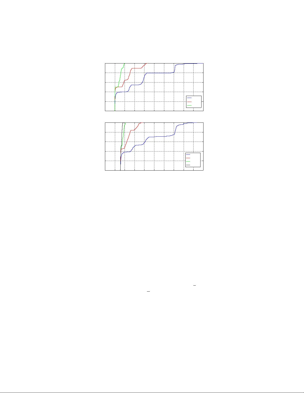
RANDOM PER TURBA TION OF LO W RANK MA TRICES: IMPR O VING CLASSICAL BOUNDS SEAN O’ROURKE, V AN VU, AND KE W ANG Abstract. Matrix perturbation inequalities, such as W eyl’s theorem (con- cerning the singular v alues) and the Davis-Kahan theorem (concerning the singular v ectors), play essen tial roles in quantitativ e science; in particular, these b ounds have found application in data analysis as well as related areas of engineering and computer science. In man y situations, the p erturbation is assumed to b e random, and the original matrix has certain structural properties (such as having low rank). W e show that, in this scenario, classical p erturbation results, suc h as W eyl and Da vis-Kahan, can b e impro v ed significan tly . W e b eliev e man y of our new bounds are close to optimal and also discuss some applications. 1. Introduction The singular v alue decomposition of a real m × n matrix A is a factorization of the form A = U Σ V T , where U is a m × m orthogonal matrix, Σ is a m × n rectangular diagonal matrix with non-negative real num b ers on the diagonal, and V T is an n × n orthogonal matrix. The diagonal entries of Σ are known as the singular values of A . The m columns of U are the left-singular ve ctors of A , while the n columns of V are the right-singular ve ctors of A . If A is symmetric, the singular v alues are given b y the absolute v alue of the eigenv alues, and the singular vectors can b e expressed in terms of the eigenv ectors of A . Here, and in the sequel, whenever we write singular ve ctors , the reader is free to interpret this as left-singular v ectors or righ t-singular vectors pro vided the same choice is made throughout the pap er. An important problem in statistics and numerical analysis is to compute the first k singular v alues and v ectors of an m × n matrix A . In particular, the largest few singular v alues and corresp onding singular vectors are typically the most im- p ortan t. Among others, this problem lies at the heart of Principal Component Analysis (PCA), which has a very wide range of applications (for many examples, see [27, 35] and the references therein) and in the closely related low rank appro x- imation procedure often used in theoretical computer science and com binatorics. In application, the dimensions m and n are t ypically large and k is small, often a fixed constant. 1.1. The p erturbation problem. A problem of fundamental importance in quan- titativ e science (including pure and applied mathematics, statistics, engineering, and computer science) is to estimate how a small p erturbation to the data effects 2010 Mathematics Subje ct Classific ation. 65F15 and 15A42. Key wor ds and phr ases. Singular v alues, singular v ectors, singular v alue decomposition, ran- dom perturbation, random matrix. S. O’Rourke is supp orted by grant AF OSAR-F A-9550-12-1-0083. V. V u is supported by research grants DMS-0901216 and AFOSAR-F A-9550-09-1-0167. 1 2 S. O’R OURKE, V AN VU, AND KE W ANG the singular v alues and singular v ectors. This problem has b een discussed in virtu- ally ev ery text bo ok on quantitativ e linear algebra and numerical analysis (see, for instance, [8, 23, 24, 47]), and is the main fo cus of this pap er. W e mo del the problem as follo ws. Consider a real (deterministic) m × n matrix A with singular v alues σ 1 ≥ σ 2 ≥ · · · ≥ σ min { m,n } ≥ 0 and corresp onding singular v ectors v 1 , v 2 , . . . , v min { m,n } . W e will call A the data matrix. In general, the vector v i is not unique. Ho w ev er, if σ i has m ultiplicit y one, then v i is determined up to sign. Instead of A , one often needs to work with A + E , where E represents the p erturbation matrix. Let σ 0 1 ≥ · · · ≥ σ 0 min { m,n } ≥ 0 denote the singular v alues of A + E with corresp onding singular v ectors v 0 1 , . . . , v 0 min { m,n } . In this pap er, we address the follo wing tw o questions. Question 1. When is v 0 i a go o d appr oximation of v i ? Question 2. When is σ 0 i a go o d appr oximation of σ i ? These tw o questions are classically addressed by the Davis-Kahan-W edin sine theorem and W eyl’s inequalit y . Let us begin with the first question in the case when i = 1. A canonical wa y (coming from the numerical analysis literature; see for instance [22]) to measure the distance b etw een tw o unit vectors v and v 0 is to lo ok at sin ∠ ( v , v 0 ), where ∠ ( v , v 0 ) is the angle b et w een v and v 0 tak en in [0 , π / 2]. It has b een observed by numerical analysts (in the setting where E is deterministic) for quite some time that the key parameter to consider in the b ound is the gap (or separation) σ 1 − σ 0 2 . The first result in this direction is the famous Da vis-Kahan sine θ theorem [20] for Hermitian matrices. A version for the singular vectors was pro ved later b y W edin [57]. Throughout the pap er, w e use k M k to denote the sp ectral norm of a matrix M . That is, k M k is the largest singular v alue of M . Theorem 3 (Davis-Kahan, W edin; sine theorem; Theorem V.4.4 from [47]) . (1) sin ∠ ( v 1 , v 0 1 ) ≤ k E k σ 1 − σ 0 2 . In certain cases, such as when E is random, it is more natural to deal with the gap (2) δ := σ 1 − σ 2 , b et ween the first and second singular v alues of A instead of σ 1 − σ 0 2 . In this case, Theorem 3 implies the following bound. Theorem 4 (Mo dified sine theorem) . sin ∠ ( v 1 , v 0 1 ) ≤ 2 k E k δ . Remark 5. Theorem 4 is trivially true when δ ≤ 2 k E k since sine is alw ays b ounded ab o ve by one. In other words, even if the vector v 0 1 is not uniquely determined, the b ound is still true for an y c hoice of v 0 1 . On the other hand, when δ > 2 k E k , the pro of of Theorem 4 reveals that the vector v 0 1 is uniquely determined up to sign. RANDOM PER TURBA TION OF LOW RANK MA TRICES 3 As the next example sho ws, the b ound in Theorem 4 is sharp, up to the constant 2. Example 6. Let 0 < ε < 1 / 2, and take A :=  1 + ε 0 0 1 − ε  , E :=  − ε ε ε ε  . Then σ 1 = 1 + ε , σ 2 = 1 − ε with v 1 = (1 , 0) T and v 2 = (0 , 1) T . Hence, δ = 2 ε . In addition, A + E =  1 ε ε 1  , and a simple computation rev eals that σ 0 1 = 1+ ε , σ 0 2 = 1 − ε but v 0 1 = (1 / √ 2 , 1 / √ 2) T and v 0 2 = (1 / √ 2 , − 1 / √ 2) T . Th us, sin ∠ ( v 1 , v 0 1 ) = 1 √ 2 = k E k δ since k E k = √ 2 ε . More generally , one can consider approximating the i -th singular v ector v i or the space spanned by the first i singular vectors Span { v 1 , . . . , v i } . Naturally , in these cases, a version of Theorem 4 requires one to consider the gaps δ i := σ i − σ i +1 ; see Theorems 19 and 21 b elo w for details. Question 2 is addressed by W eyl’s inequality . In particular, W eyl’s perturbation theorem [58] gives the following deterministic b ound for the singular v alues (see [47, Theorem IV.4.11] for a more general p erturbation bound due to Mirsky [40]). Theorem 7 (W eyl’s b ound) . max 1 ≤ i ≤ min { m,n } | σ i − σ 0 i | ≤ k E k . F or more discussions concerning general p erturbation b ounds, w e refer the reader to [10, 47] and references therein. W e now pause for a moment to prov e Theorem 4. Pr o of of The or em 4. If δ ≤ 2 k E k , the theorem is trivially true since sine is alwa ys b ounded abov e b y one. Th us, assume δ > 2 k E k . By Theorem 7, we ha v e σ 0 1 − σ 0 2 ≥ δ − 2 k E k > 0 , and hence the singular v ectors v 1 and v 0 1 are uniquely determined up to sign. By another application of Theorem 7, we obtain δ = σ 1 − σ 2 ≤ σ 1 − σ 0 2 + k E k . Rearranging the inequality , we ha v e σ 1 − σ 0 2 ≥ δ − k E k ≥ 1 2 δ > 0 . Therefore, by (1), we conclude that sin ∠ ( v 1 , v 0 1 ) ≤ k E k σ 1 − σ 0 2 ≤ 2 k E k δ , and the pro of is complete.  4 S. O’R OURKE, V AN VU, AND KE W ANG 1.2. The random setting. Let us no w focus on the matrices A and E . It has b ecome common practice to assume that the p erturbation matrix E is random. F urthermore, researc hers ha ve observed that data matrices are usually not arbitrary . They often possess certain structural properties. Among these properties, one of the most frequently seen is ha ving lo w rank (see, for instance, [14, 15, 16, 19, 51] and references therein). The goal in this pap er is to sho w that in this situation, one c an significan tly impro ve classical results lik e Theorems 4 and 7. T o give a quick example, let us assume that A and E are n × n matrices and that E is a random Bernoulli matrix, i.e., its en tries are indep enden t and identically distributed (iid) random v ariables that take v alues ± 1 with probabilit y 1 / 2. It is well known that in this case k E k = (2 + o (1)) √ n with high probabilit y 1 [7, Chapter 5]. Thus, the abov e t wo theorems imply the following. Corollary 8. If E is an n × n Bernoul li 2 r andom matrix, then, for any η > 0 , with pr ob ability 1 − o (1) , max 1 ≤ i ≤ n | σ i − σ 0 i | ≤ (2 + η ) √ n, and (3) sin ∠ ( v 1 , v 0 1 ) ≤ 2(2 + η ) √ n δ . Among others, this shows that we must hav e δ > 2(2 + η ) √ n in order for the b ound in (3) to b e nontrivial. It turns out that the b ounds in Corollary 8 are far from b eing sharp. Indeed, w e presen t the results of a numerical sim ulation for A b eing a n × n matrix of rank 2 when n = 400, δ = 8, and where E is a random Bernoulli matrix. It is easy to see that for the parameters n = 400 and δ = 8, Corollary 8 does not giv e a useful b ound (since √ n δ = 2 . 5 > 1). How ev er, Figure 1 shows that, with high probabilit y , sin ∠ ( v 1 , v 0 1 ) ≤ 0 . 2, whic h means v 0 1 appro ximates v 1 with a relativ ely small error. Our main results attempt to address this inefficiency in the Davis-Kahan-W edin and W eyl b ounds and provide sharp er b ounds than those given in Corollary 8. As a concrete example, in the case when E is a random Bernoulli matrix, our results imply the following bounds. Theorem 9. L et E b e a n × n Bernoul li r andom matrix, and let A b e a n × n matrix with r ank r . F or every ε > 0 ther e exists c onstants C 0 , δ 0 > 0 (dep ending only on ε ) such that if δ ≥ δ 0 and σ 1 ≥ max { n, √ nδ } , then, with pr ob ability at le ast 1 − ε , sin ∠ ( v 1 , v 0 1 ) ≤ C √ r δ . Theorem 10. L et E b e an n × n Bernoul li r andom matrix, and let A b e an n × n matrix with r ank r satisfying σ 1 ≥ n . F or every ε > 0 , ther e exists a c onstant C 0 > 0 (dep ending only on ε ) such that, with pr ob ability at le ast 1 − ε , σ 1 − C ≤ σ 0 1 ≤ σ 1 + C √ r . 1 W e use asymptotic notation under the assumption that n → ∞ . Here w e use o (1) to denote a term which tends to zero as n tends to infinity . 2 More generally , Corollary 8 applies to a large class of random matrices with indep enden t entries. Indeed, the results in [7, Chapter 5] and hence Corollary 8 hold when E is any n × n random matrix whose entries are iid random v ariables with zero mean, unit v ariance (which is just a matter of normalization), and bounded fourth moment. RANDOM PER TURBA TION OF LOW RANK MA TRICES 5 0 0.1 0.2 0.3 0.4 0.5 0.6 0.7 0.8 0.9 1 0 0.2 0.4 0.6 0.8 1 sin ! (v 1 , v 1 ’) Comulative Distribution Function n = 400, rank = 2, " = gap " = 2 " = 4 " = 8 0 0.1 0.2 0.3 0.4 0.5 0.6 0.7 0.8 0.9 1 0 0.2 0.4 0.6 0.8 1 sin ! (v 1 , v 1 ’) Comulative Distribution Function n = 1000, rank = 2, " = gap " = 2 " = 5 " = 10 " = 15 Figure 1. The cumulativ e distribution functions of sin ∠ ( v 1 , v 0 1 ) where A is a n × n deterministic matrix with rank 2 ( n = 400 for the figure on top and n = 1000 for the one b elow) and the noise E is a Bernoulli random matrix, ev aluated from 400 samples (top figure) and 300 samples (b ottom figure). In b oth figures, the largest singular v alue of A is taken to b e 200. In particular, when the rank r is significan tly smaller than n , the b ounds in Theorems 9 and 10 are significantly better than those app earing in Corollary 8. The intuition behind Theorems 9 and 10 comes from the following heuristic of the second author. If A has rank r , all actions of A focus on an r dimensional subspace; in tuitively then, E must act like an r dimensional random matrix rather than an n dimensional one. This means that the r e al dimension of the problem is r , not n . While it is clear that one cannot automatically ignore the (rather wild) action of E outside the range of A , this in tuition, if true, explains the app earance of the √ r factor in the b ounds of Theorems 9 and 10 instead of the √ n factor app earing in Corollary 8. While Theorems 9 and 10 are stated only for Bernoulli random matrices E , our main results actually hold under very mild assumptions on A and E . As a matter of fact, in the strongest results, we will not even need the entries of E to b e indep enden t. 1.3. Preliminaries: Mo dels of random noise. W e now state the assumptions w e require for the random matrix E . While there are man y models of random ma- trices, we can capture almost all natu ral mo dels by fo cusing on a common prop ert y . 6 S. O’R OURKE, V AN VU, AND KE W ANG Definition 11. W e sa y the m × n random matrix E is ( C 1 , c 1 , γ )-concentrated if for all unit vectors u ∈ R m , v ∈ R n , and every t > 0, (4) P ( | u T E v | > t ) ≤ C 1 exp( − c 1 t γ ) . The key parameter is γ . It is easy to verify the following fact, whic h asserts that the concentration property is closed under addition. F act 12. If E 1 is ( C 1 , c 1 , γ ) -c onc entr ate d and E 2 is ( C 2 , c 2 , γ ) -c onc entr ate d, then E 3 = E 1 + E 2 is ( C 3 , c 3 , γ ) -c onc entr ate d for some C 3 , c 3 dep ending on C 1 , c 1 , C 2 , c 2 . F urthermore, the concentration prop ert y guaran tees a bound on k E k . A stan- dard net argument (see Lemma 28) shows F act 13. If E is ( C 1 , c 1 , γ ) -c onc entr ate d then ther e ar e c onstants C 0 , c 0 > 0 such that P ( k E k ≥ C 0 n 1 /γ ) ≤ C 1 exp( − c 0 n ) . F or readers not familiar with random matrix theory , let us p oint out wh y the concen tration property is expected to hold for man y natural mo dels. If E is random and v is fixed, then the v ector E v must lo ok random. It is well known that in a high dimensional space, a random isotropic v ector, with v ery high probability , is nearly orthogonal to an y fixed vector. Th us, one exp ects that very likely , the inner pro duct of u and E v is small. Definition 11 is a w a y to express this observ ation quan titatively . It turns out that all random matrices with indep enden t entries satisfying a mild condition hav e the concentration prop ert y . Indeed, if E ij denotes the ( i, j )-entry of E and the entries of E are assumed to b e indep enden t, then the bilinear form u T E v = m X i =1 n X j =1 u i E ij v j is just a sum of indep enden t random v ariables. If, in addition, the entries of E hav e mean zero, then, by linearit y , u T E v also has mean zero. Hence, (4) can b e viewed as a concen tration inequality , which expresses ho w the sum of indep enden t random v ariables deviates from its mean. With this interpretation in mind, many mo dels of random matrices can b e shown to satisfy (4). In particular, Lemma 34 shows that if E is a n × n Bernoulli random matrix, then E is  2 , 1 2 , 2  -concen trated, and k E k ≤ 3 √ n with high probabilit y [53, 54]. How ever, a con venien t feature of the definition is that indep endence b et ween the en tries is not a requirement. F or instance, it is easy to sho w that a random orthogonal matrix satisfies the concen tration property . W e con tin ue the discussion of the ( C 1 , c 1 , γ )-concentration prop ert y (Definition 11) in Section 6. 2. Main resul ts W e now state our main results. W e b egin with an extension of Theorem 9. Theorem 14. Assume that E is ( C 1 , c 1 , γ ) -c onc entr ate d for a trio of c onstants C 1 , c 1 , γ > 0 , and supp ose A has r ank r . Then, for any t > 0 , (5) sin ∠ ( v 1 , v 0 1 ) ≤ 4 √ 2  tr 1 /γ δ + k E k σ 1 + k E k 2 σ 1 δ  with pr ob ability at le ast (6) 1 − 54 C 1 exp  − c 1 δ γ 8 γ  − 2 C 1 9 2 r exp  − c 1 r t γ 4 γ  . RANDOM PER TURBA TION OF LOW RANK MA TRICES 7 Remark 15. Using F act 13, one can replace k E k on the righ t-hand side of (5) b y C 0 n 1 /γ , which yields that sin ∠ ( v 1 , v 0 1 ) ≤ 4 √ 2  tr 1 /γ δ + C 0 n 1 /γ σ 1 + C 0 2 n 2 /γ σ 1 δ  with probability at least 1 − 54 C 1 exp  − c 1 δ γ 8 γ  − 2 C 1 9 2 r exp  − c 1 r t γ 4 γ  − C 1 exp( − c 0 n ) . Ho wev er, we prefer to state our theorems in the form of Theorem 14, as the b ound C 0 n 1 /γ , in many cases, may not be optimal. Because Theorem 14 is stated in such generality , the b ounds can b e difficult to in terpret. F or example, it is not completely obvious when the probability in (6) is close to one. Roughly sp eaking, the tw o error terms in the probability b ound are con trolled by the gap δ and the parameter t (which can b e taken to be any p ositiv e v alue). Sp ecifically , the first term (7) 54 C 1 exp  − c 1 δ γ 8 γ  go es to zero as δ gets larger, and the second term (8) 2 C 1 9 2 r exp  − c 1 r t γ 4 γ  go es to zero as t tends to infinity . As a consequence, w e obtain the following immediate corollary of Theorem 14 (and Lemma 36) in the case when the en tries of E are indep enden t. Corollary 16. Assume that E is an m × n r andom matrix with indep endent entries which have me an zer o and ar e b ounde d almost sur ely in magnitude by K for some K > 0 . Supp ose A has r ank r . Then for every ε > 0 , ther e exists C 0 , c 0 , δ 0 > 0 (dep ending only on ε and K ) such that if δ ≥ δ 0 , then (9) sin ∠ ( v 1 , v 0 1 ) ≤ C 0  √ r δ + k E k σ 1 + k E k 2 σ 1 δ  with pr ob ability at le ast 1 − ε . The first term √ r δ on the right-hand side of (9) is precisely the conjectured optimal b ound coming from the intuition discussed ab o v e. The second term k E k σ 1 is necessary . If k E k  σ 1 , then the intensit y of the noise is muc h stronger than the strongest signal in the data matrix, so E would corrupt A completely . Thus in order to retain crucial information ab out A , it seems necessary to assume k E k < σ 1 . W e are not absolutely sure ab out the necessit y of the third term k E k 2 σ 1 δ , but under the condition k E k  σ 1 , this term is sup erior to the Davis-Kahan-W edin b ound k E k δ app earing in Theorem 4. While it remains an op en question to determine whether the b ounds in Theorem 14 are optimal, w e do note that in certain situations the b ounds are close to optimal. Indeed, in [9], the eigen v ectors of p erturb ed random matrices are studied, and, under v arious tec hnical assumptions on the matrices A and E , the results in [9] giv e the exact asymptotic b eha vior of the dot pro duct | v 1 · v 0 1 | . Rewriting the dot pro duct in terms of cosine (and further expressing the v alue in terms of sine), we 8 S. O’R OURKE, V AN VU, AND KE W ANG find that the b ounds in (5) match the exact asymptotic b ehavior obtained in [9], up to constan t factors. Similar results in [43] also match the b ound in (5), up to constan t factors, in the case when E is a Wigner random matrix and A has rank one. Corollary 16 pro vides a b ound which holds with probability at least 1 − ε . As another consequence of Theorem 14, w e obtain the follo wing b ound whic h holds with probability con v erging to 1. Corollary 17. Assume that E is an m × n r andom matrix with indep endent entries which have me an zer o and ar e b ounde d almost sur ely in magnitude by K for some K > 0 . Supp ose A has r ank r . Then ther e exists C 0 > 0 (dep ending only on K ) such that if α n is any se quenc e of p ositive values c onver ging to infinity and δ ≥ α n , then sin ∠ ( v 1 , v 0 1 ) ≤ C 0  α n √ r δ + k E k σ 1 + k E k 2 σ 1 δ  with pr ob ability 1 − o (1) . Her e, the r ate of c onver genc e implicit in the o (1) notation dep ends on K and α n . Before con tin uing, we pause to make one final remark regarding Corollaries 16 and 17. In stating our main results b elo w, we will alwa ys state them in the generality of Theorem 14. How ever, each of the results can b e sp ecialized in several different directions similar to what w e ha v e done in Corollaries 16 and 17. In the interest of space, we will not alwa ys state all such corollaries. W e are able to extend Theorem 14 in tw o different wa ys. First, w e can b ound the angle b et w een v j and v 0 j for any index j . Second, and more imp ortantly , w e can b ound the angle b et w een the subspaces spanned by { v 1 , . . . , v j } and { v 0 1 , . . . , v 0 j } , resp ectiv ely . As the pro jection on to the subspaces spanned by the first few singular v ectors (i.e., low rank approximation) pla ys an imp ortant role in a v ast colle ction of problems, this result p oten tially has a large num b er of applications. x W e b egin by bounding the largest principal angle b et w een (10) V := Span { v 1 , . . . , v j } and V 0 := Span { v 0 1 , . . . , v 0 j } for some in teger 1 ≤ j ≤ r , where r is the rank of A . Let us recall that if U and V are t w o subspaces of the same dimension, then the (principal) angle b et w een them is defined as (11) sin ∠ ( U, V ) := max u ∈ U ; u 6 =0 min v ∈ V ; v 6 =0 sin ∠ ( u, v ) = k P U − P V k = k P U ⊥ P V k , where P W denotes the orthogonal pro jection onto subspace W . Theorem 18. Assume that E is ( C 1 , c 1 , γ ) -c onc entr ate d for a trio of c onstants C 1 , c 1 , γ > 0 . Supp ose A has r ank r , and let 1 ≤ j ≤ r b e an inte ger. Then, for any t > 0 , (12) sin ∠ ( V , V 0 ) ≤ 4 p 2 j  tr 1 /γ δ j + k E k 2 σ j δ j + k E k σ j  , with pr ob ability at le ast (13) 1 − 6 C 1 9 j exp − c 1 δ γ j 8 γ ! − 2 C 1 9 2 r exp  − c 1 r t γ 4 γ  , wher e V and V 0 ar e the j -dimensional subsp ac es define d in (10) . RANDOM PER TURBA TION OF LOW RANK MA TRICES 9 The error terms in (13) (as well as all other probability b ounds app earing in our main results) can b e controlled in a similar fashion as the error terms (7) and (8). Indeed, the first error term in (13) is con trolled b y the gap δ j and the second term is controlled b y the parameter t . W e b elieve the factor of √ j in (12) is suboptimal and is simply an artifact of our pro of. How ever, in many applications j is significantly smaller than the dimension of the matrices, making the contribution from this term negligible. F or comparison, w e present an analogue of Theorem 4, whic h follows from the Da vis-Kahan-W edin sine theorem [47, Theorem V.4.4], using the same argument as in the pro of of Theorem 4. Theorem 19 (Mo dified Davis-Kahan-W edin sine theorem: singular space) . Sup- p ose A has r ank r , and let 1 ≤ j ≤ r b e an inte ger. Then, for an arbitr ary matrix E , sin ∠ ( V , V 0 ) ≤ 2 k E k δ j , wher e V and V 0 ar e the j -dimensional subsp ac es define d in (10) . It remains an op en question to give an optimal version of Theorem 18 for sub- spaces corresp onding to an arbitrary set of singular v alues. How ev er, we can use Theorem 18 rep eatedly to obtain b ounds for the case when one considers a few in terv als of singular v alues. F or instance, b y applying Theorem 18 twice, we obtain the following result. Denote δ 0 := δ 1 . Corollary 20. Assume that E is ( C 1 , c 1 , γ ) -c onc entr ate d for a trio of c onstants C 1 , c 1 , γ > 0 . Supp ose A has r ank r , and let 1 < j ≤ l ≤ r b e inte gers. Then, for any t > 0 , (14) sin ∠ ( V , V 0 ) ≤ 8 √ 2 l  tr 1 /γ δ j − 1 + tr 1 /γ δ l + k E k 2 σ j − 1 δ j − 1 + k E k 2 σ l δ l + k E k σ l  , with pr ob ability at le ast 1 − 6 C 1 9 j − 1 exp − c 1 δ γ j − 1 8 γ ! − 6 C 1 9 l exp  − c 1 δ γ l 8 γ  − 4 C 1 9 2 r exp  − c 1 r t γ 4 γ  , wher e (15) V := Span { v j , . . . , v l } and V 0 := Span { v 0 j , . . . , v 0 l } . Pr o of. Let V 1 := Span { v 1 , . . . , v l } , V 0 1 := Span { v 0 1 , . . . , v 0 l } , V 2 := Span { v 1 , . . . , v j − 1 } , V 0 2 := Span { v 0 1 , . . . , v 0 j − 1 } . F or any subspace W , let P W denote the orthogonal pro jection on to W . It follows that P W ⊥ = I − P W , where I denotes the identit y matrix. By definition of the subspaces V , V 0 , we ha v e P V = P V 1 P V ⊥ 2 and P V 0 = P V 0 1 P V 0⊥ 2 . 10 S. O’R OURKE, V AN VU, AND KE W ANG Th us, by (11), we obtain sin ∠ ( V , V 0 ) = k P V 1 P V ⊥ 2 − P V 0 1 P V 0⊥ 2 k ≤ k P V 1 P V ⊥ 2 − P V 0 1 P V ⊥ 2 k + k P V 0 1 P V ⊥ 2 − P V 0 1 P V 0⊥ 2 k ≤ k P V 1 − P V 0 1 k + k P V 2 − P V 0 2 k = sin ∠ ( V 1 , V 0 1 ) + sin ∠ ( V 2 , V 0 2 ) . Theorem 18 can now b e in vok ed to b ound sin ∠ ( V 1 , V 0 1 ) and sin ∠ ( V 2 , V 0 2 ), and the claim follows.  Again, the factor of √ l app earing in (14) follo ws from the analogous factor app earing in (12). Indeed, if this factor could b e remov ed from (12), then the pro of ab o ve shows that it w ould also b e remov ed from (14). F or comparison, we present the following version of Theorem 4, which follows Theorem 19 and the argument abov e. Again denote δ 0 := δ 1 . Theorem 21 (Mo dified Davis-Kahan-W edin sine theorem: singular space) . Sup- p ose A has r ank r , and let 1 ≤ j ≤ l ≤ r b e inte gers. Then, for an arbitr ary matrix E , sin ∠ ( V , V 0 ) ≤ 4 k E k min { δ j − 1 , δ l } , wher e V and V 0 ar e define d in (15) . W e now consider the problem of approximating the j -th singular vector v j re- cursiv ely in terms of the b ounds for sin ∠ ( v i , v 0 i ), i < j . Theorem 22. Assume that E is ( C 1 , c 1 , γ ) -c onc entr ate d for a trio of c onstants C 1 , c 1 , γ > 0 . Supp ose A has r ank r , and let 1 ≤ j ≤ r b e an inte ger. Then, for any t > 0 , sin ∠ ( v j , v 0 j ) ≤ 4 √ 2   j − 1 X i =1 sin 2 ∠ ( v i , v 0 i ) ! 1 / 2 + tr 1 /γ δ j + k E k 2 σ j δ j + k E k σ j   with pr ob ability at le ast 1 − 6 C 1 9 j exp − c 1 δ γ j 8 γ ! − 2 C 1 9 2 r exp  − c 1 r t γ 4 γ  . The b ound in Theorem 22 dep ends inductively on the b ounds for sin 2 ∠ ( v i , v 0 i ), i = 1 , . . . , j − 1, and as such, we do not believe it to b e sharp. The bound does, ho wev er, impro ve upon a similar recursive bound presented in [53]. Finally , let us present the general form of Theorem 10 for singular v alues. Read- ers can compare the result with the classical b ound in Theorem 7. Theorem 23. Assume that E is ( C 1 , c 1 , γ ) -c onc entr ate d for a trio of c onstants C 1 , c 1 , γ > 0 . Supp ose A has r ank r , and let 1 ≤ j ≤ r b e an inte ger. Then, for any t > 0 , (16) σ 0 j ≥ σ j − t with pr ob ability at le ast 1 − 2 C 1 9 j exp  − c 1 t γ 4 γ  , RANDOM PER TURBA TION OF LOW RANK MA TRICES 11 and (17) σ 0 j ≤ σ j + tr 1 /γ + 2 p j k E k 2 σ 0 j + j k E k 3 σ 0 j 2 with pr ob ability at le ast 1 − 2 C 1 9 2 r exp  − c 1 r t γ 4 γ  . Remark 24. Notice that the upp er b ound for σ 0 j giv en in (17) inv olves 1 /σ 0 j . In man y situations, the low er b ound in (16) can b e used to provide an upp er b ound for 1 /σ 0 j . W e conjecture that the factors of √ j and j app earing in (17) are not needed and are simply an artifact of our pro of. In applications, j is typically muc h smaller than the dimension, often making the contribution from these terms negligible. T o illustrate this p oin t, consider the follo wing example when r = O (1). Let A and E be symmetric matrices, and assume the en tries on and ab ov e the diagonal of E are independent random v ariables. Suc h a matrix E is known as a Wigner matrix, and the eigen v alues of perturb ed Wigner matrices ha ve been w ell-studied in the random matrix theory literature; see, for instance, [31, 44] and references therein. In particular, the results in [31, 44] giv e the asymptotic lo cation of the largest r eigen v alues as well as their join t fluctuations. These exact asymptotic results imply that, in this setting, the b ounds app earing in Theorem 23 are sharp, up to constant factors. As the b ounds in Theorem 23 are fairly general, let us state a corollary in the case when the entries of E are indep enden t random v ariables. Corollary 25. Assume that E is an m × n r andom matrix with indep endent entries which have me an zer o and ar e b ounde d almost sur ely in magnitude by K for some K > 0 . Supp ose A has r ank r . Then, for every ε > 0 , ther e exists C 0 > 0 (dep ending only on ε and K ) such that, with pr ob ability at le ast 1 − ε , (18) σ j − C 0 p j ≤ σ 0 j ≤ σ j + C 0 √ r + 2 p j k E k 2 σ 0 j + j k E k 3 σ 0 j 2 for al l 1 ≤ j ≤ r . Corollary 25 is an immediate consequence of Theorem 23, Lemma 36, and the union bound. In particular, the b ound in (18) holds for all v alues of 1 ≤ j ≤ r sim ultaneously with probability at least 1 − ε . 2.1. Related results. T o conclude this section, let us men tion a few related re- sults. In [53], the second author managed to prov e sin 2 ∠ ( v 1 , v 0 1 ) ≤ C √ r log n δ under certain conditions. While the right-hand side is quite close to the optimal form in Theorem 9, the main problem here is that in the left-hand side one needs to square the sine function. The b ound for sin ∠ ( v i , v 0 i ) with i ≥ 2 w as done by an inductiv e argumen t and w as rather complicated. Finally , the problem of estimating the singular v alues w as not addressed at all in [53]. 12 S. O’R OURKE, V AN VU, AND KE W ANG Related results ha v e also been obtained in the case where the random matrix E con tains Gaussian entries. In [56], R. W ang estimates the non-asymptotic dis- tribution of the singular v ectors when the en tries of E are iid standard normal random v ariables. Recen tly , Allez and Bouchaud hav e studied the eigenv ector dy- namics of A + E when A is a real symmetric matrix and E is a symmetric Bro wnian motion (that is, E is a diffusiv e matrix pro cess constructed from a family of in- dep enden t real Brownian motions) [2]. Our results also seems to hav e a close tie to the study of spiked cov ariance matrices, where a different kind of p erturbation has b een considered; see [12, 26, 41] for details. It w ould b e interesting to find a common generalization for these problems. 3. O ver view and outline W e now briefly give an ov erview of the pap er and discuss some of the k ey ideas b ehind the pro of of our main results. F or simplicity , let us assume that A and E are n × n real symmetric matrices. (In fact, we will symmetrize the problem in Section 4 below.) Let σ 1 ≥ · · · ≥ σ n b e the eigen v alues of A with corresp onding (orthonormal) eigenv ectors v 1 , . . . , v n . Let σ 0 1 b e the largest eigenv alue of A + E with corresp onding (unit) eigenv ector v 0 1 . Supp ose w e wish to b ound sin ∠ ( v 1 , v 0 1 ) (from Theorem 14). Since sin 2 ∠ ( v 1 , v 0 1 ) = 1 − cos 2 ∠ ( v 1 , v 0 1 ) = n X k =2 | v k · v 0 1 | 2 , it suffices to b ound | v k · v 0 1 | for k = 2 , . . . , n . Let us consider the case when k = 2 , . . . , r . In this case, we ha v e v T k ( A + E ) v 0 1 − v T k Av 0 1 = v T k E v 0 1 . Since ( A + E ) v 0 1 = σ 0 1 v 0 1 and v T k A = σ k v k , we obtain | σ 0 1 − σ k || v k · v 0 1 | ≤ | v T k E v 0 1 | . Th us, the problem of b ounding | v k · v 0 1 | reduces to obtaining an upp er bound for | v T k E v 0 1 | and a low er b ound for the gap | σ 0 1 − σ k | . W e will obtain b ounds for b oth of these terms by using the concentration prop ert y (Definition 11). More generally , in Section 4, we will apply the concentration prop ert y to obtain lo wer b ounds for the gaps σ 0 j − σ k when j < k , which will hold with high probabilit y . Let us illustrate this by no w considering the gap σ 0 1 − σ 2 . Indeed, w e note that σ 0 1 = k A + E k ≥ v T 1 ( A + E ) v 1 = σ 1 + v T 1 E v 1 . Applying the concentration property (4), we see that σ 0 1 > σ 1 − t with probability at least 1 − C 1 exp( − c 1 t γ ). As δ := σ 1 − σ 2 , we in fact observe that σ 0 1 − σ 2 = σ 0 1 − σ 1 + δ > δ − t. Th us, if δ is sufficiently large, we ha v e (sa y) σ 0 1 − σ 2 ≥ δ / 2 with high probability . In Section 5, w e will again apply the concentration prop ert y to obtain upp er b ounds for terms of the form v k E v 0 j . A t the end of Section 5, w e com bine these b ounds to complete the pro of of Theorems 14, 18, 22, and 23. In Section 6, w e discuss the ( C 1 , c 1 , γ )-concentration prop erty (Definition 11). In particular, we generalize some previous results obtained by the second author in [53]. Finally , in Section 7, we presen t some applications of our main results. RANDOM PER TURBA TION OF LOW RANK MA TRICES 13 Singular subspace p erturbation bounds are applicable to a wide v ariety of prob- lems. F or instance, [13] discuss several applications of these bounds to high- dimensional statistics including high dimensional clustering, canonical correlation analysis (CCA), and matrix recov ery . In Section 7, we show how our results can b e applied to the matrix recov ery problem. The general matrix recov ery problem is the following. A is a large matrix. Ho w ev er, the matrix A is unkno wn to us. W e can only observe its noisy p erturbation A + E , or in some cases just a small p ortion of the p erturbation. Our goal is to reconstruct A or estimate an imp ortan t param- eter as accurately as p ossible from this observ ation. F urthermore, several problems from combinatorics and theoretical computer science can also be formulated in this setting. Sp ecial instances of the matrix recov ery problem ha v e been in v estigated b y many researchers using sp ectral tec hniques and combinatorial argumen ts in in- genious w a ys [1, 3, 4, 5, 11, 14, 15, 16, 17, 18, 21, 28, 29, 32, 33, 34, 37, 39, 42, 45]. W e prop ose the following simple analysis: if A has rank r and 1 ≤ j ≤ r , then the pro jection of A + E on the subspace V 0 spanned b y the first j singular vectors of A + E is close to the pro jection of A + E onto the subspace V spanned by the first j singular vectors of A , as our new results show that V and V 0 are v ery close. Moreo ver, w e can also show that the pro jection of E onto V is typically small. Th us, by pro jecting A + E onto V 0 , we obtain a go od approximation of the rank j approximation of A . In certain cases, we can rep eat the ab o v e op eration a few times to obtain sufficient information to recov er A completely or to estimate the required parameter with high accuracy and certaint y . 4. Preliminar y tools In this section, w e present some of the preliminary to ols we will need to prov e Theorems 14, 18, 22, and 23. T o b egin, we define the ( m + n ) × ( m + n ) symmetric blo c k matrices (19) ˜ A :=  0 A A T 0  and ˜ E :=  0 E E T 0  . W e will work with the matrices ˜ A and ˜ E instead of A and E . If A T u = σ v and Av = σu , then ˜ A T ( u T , v T ) T = σ ( u T , v T ) T and ˜ A T ( u T , − v T ) T = − σ ( u T , − v T ) T . In particular, the non-zero eigenv alues of ˜ A are ± σ 1 , . . . , ± σ r and the eigenv ectors are formed from the left and right singular vectors of A . Similarly , the non-trivial eigen v alues of ˜ A + ˜ E are ± σ 0 1 , . . . , ± σ 0 min { m,n } (some of which may be zero) and the eigen vectors are formed from the left and right singular v ectors of A + E . Along these lines, w e introduce the following notation, whic h differs from the notation used abov e. The non-zero eigenv alues of ˜ A will be denoted by ± σ 1 , . . . , ± σ r with orthonormal eigenv ectors u k , k = ± 1 , . . . , ± r such that ˜ Au k = σ k u k , ˜ Au − k = − σ k u − k , k = 1 , . . . , r. Let v 1 , . . . , v j b e the orthonormal eigenv ectors of ˜ A + ˜ E corresp onding to the j - largest eigenv alues λ 1 ≥ · · · ≥ λ j . In order to prov e Theorems 14, 18, 22, and 23, it suffices to w ork with the eigen vectors and eigenv alues of the matrices ˜ A and ˜ A + ˜ E . Indeed, Prop osition 26 14 S. O’R OURKE, V AN VU, AND KE W ANG will b ound the angle b et ween the singular vectors of A and A + E b y the angle b et ween the corresp onding eigen vectors of ˜ A and ˜ A + ˜ E . Prop osition 26. L et u 1 , v 1 ∈ R m and u 2 , v 2 ∈ R n b e unit ve ctors. L et u, v ∈ R m + n b e given by u =  u 1 u 2  , v =  v 1 v 2  . Then sin 2 ∠ ( u 1 , v 1 ) + sin 2 ∠ ( u 2 , v 2 ) ≤ 2 sin 2 ∠ ( u, v ) . Pr o of. Since k u k 2 = k v k 2 = 2, we ha v e cos 2 ∠ ( u, v ) = 1 4 | u · v | 2 ≤ 1 2 | u 1 · v 1 | 2 + 1 2 | u 2 · v 2 | 2 . Th us, sin 2 ∠ ( u, v ) = 1 − cos 2 ∠ ( u, v ) ≥ 1 2 sin 2 ∠ ( u 1 , v 1 ) + 1 2 sin 2 ∠ ( u 2 , v 2 ) , and the claim follows.  W e no w introduce some useful lemmas. The first lemma below, states that if E is ( C 1 , c 1 , γ )-concentrated, then ˜ E is ( ˜ C 1 , ˜ c 1 , γ )-concentrated, for some new constan ts ˜ C 1 := 2 C 1 and ˜ c 1 := c 1 / 2 γ . Lemma 27. Assume that E is ( C 1 , c 1 , γ ) -c onc entr ate d for a trio of c onstants C 1 , c 1 , γ > 0 . L et ˜ C 1 := 2 C 1 and ˜ c 1 := c 1 / 2 γ . Then for al l unit ve ctors u, v ∈ R n + m , and every t > 0 , (20) P ( | u t ˜ E v | > t ) ≤ ˜ C 1 exp( − ˜ c 1 t γ ) . Pr o of. Let u =  u 1 u 2  , v =  v 1 v 2  b e unit v ectors in R m + n , where u 1 , v 1 ∈ R m and u 2 , v 2 ∈ R n . W e note that u T ˜ E v = u T 1 E v 2 + u T 2 E T v 1 . Th us, if an y of the v ectors u 1 , u 2 , v 1 , v 2 are zero, (20) follows immediately from (4). Assume all the vectors u 1 , u 2 , v 1 , v 2 are nonzero. Then | u T ˜ E v | = | u T 1 E v 2 + u T 2 E T v 1 | ≤ | u T 1 E v 2 | k u 1 kk v 2 k + | v T 1 E u 2 | k u 2 kk v 1 k . Th us, by (4), we ha v e P ( | u T ˜ E v | > t ) ≤ P  | u T 1 E v 2 | k u 1 kk v 2 k > t 2  + P  | v T 1 E u 2 | k u 2 kk v 1 k > t 2  ≤ 2 C 1 exp  − c 1 t γ 2 γ  , and the pro of of the lemma is complete.  W e will also consider the sp ectral norm of ˜ E . Since ˜ E is a symmetric matrix whose eigenv alues in absolute v alue are giv en by the singular v alues of E , it follows that (21) k ˜ E k = k E k . RANDOM PER TURBA TION OF LOW RANK MA TRICES 15 W e introduce ε -nets as a conv enien t w a y to discretize a compact set. Let ε > 0. A set X is an ε -net of a set Y if for an y y ∈ Y , there exists x ∈ X suc h that k x − y k ≤ ε . The following estimate for the maximum size of an ε -net of a sphere is well-kno wn (see for instance [52]). Lemma 28. A unit spher e in d dimensions admits an ε -net of size at most  1 + 2 ε  d . Lemmas 29, 30, and 31 below are consequences of the concentration prop ert y (20). Lemma 29. Assume that E is ( C 1 , c 1 , γ ) -c onc entr ate d for a trio of c onstants C 1 , c 1 , γ > 0 . L et A b e a m × n matrix with r ank r . L et U b e the ( m + n ) × 2 r matrix whose c olumns ar e the ve ctors u 1 , . . . , u r , u − 1 , . . . , u − r . Then, for any t > 0 , P  k U T ˜ E U k > tr 1 /γ  ≤ ˜ C 1 9 2 r exp  − ˜ c 1 r t γ 2 γ  . Pr o of. Clearly U T ˜ E U is a symmetric 2 r × 2 r matrix. Let S b e the unit sphere in R 2 r . Let N be a 1 / 4-net of S . It is easy to verify (see for instance [52]) that for an y 2 r × 2 r symmetric matrix B , k B k ≤ 2 max x ∈N | x ∗ B x | . F or any fixed x ∈ N , w e hav e P ( | x T U T ˜ E U x | > t ) ≤ ˜ C 1 exp( − ˜ c 1 t γ ) b y Lemma 27. Since |N | ≤ 9 2 r , we obtain P ( k U T ˜ E U k > tr 1 /γ ) ≤ X x ∈N P  | x T U T ˜ E U x | > 1 2 tr 1 /γ  ≤ ˜ C 1 9 2 r exp  − ˜ c 1 r t γ 2 γ  .  Lemma 30. Assume that E is ( C 1 , c 1 , γ ) -c onc entr ate d for a trio of c onstants C 1 , c 1 , γ > 0 . Supp ose A has r ank r . Then, for any t > 0 , (22) λ 1 ≥ σ 1 − t with pr ob ability at le ast 1 − ˜ C 1 exp( − ˜ c 1 t γ ) . In p articular, if σ 1 > 0 , then λ 1 ≥ σ 1 2 with pr ob ability at le ast 1 − ˜ C 1 exp  − ˜ c 1 σ γ 1 2 γ  . If, in addition, δ > 0 , then λ 1 − σ k ≥ 1 2 δ for k = 2 , . . . , r with pr ob ability at le ast 1 − ˜ C 1 exp  − ˜ c 1 δ γ 2 γ  . Pr o of. W e observe that λ 1 = k ˜ A + ˜ E k ≥ u T 1 ( ˜ A + ˜ E ) u 1 = σ 1 + u T 1 ˜ E u 1 . By Lemma 27, we hav e P ( | u T 1 ˜ E u 1 | > t ) ≤ ˜ C 1 exp( − ˜ c 1 t γ ) 16 S. O’R OURKE, V AN VU, AND KE W ANG for every t > 0, and (22) follows. If σ 1 > 0, then the b ound λ 1 ≥ σ 1 2 can b e obtained by taking t = σ 1 / 2 in (22). Assume δ > 0. T aking t = δ / 2 in (22) yields λ 1 − σ k ≥ λ 1 − σ 2 = λ 1 − σ 1 + δ ≥ δ 2 for k = 2 , . . . , r with probability at least 1 − ˜ C 1 exp  − ˜ c 1 δ γ 2 γ  .  Using the Courant minimax principle, Lemma 30 can b e generalized to the fol- lo wing. Lemma 31. Assume that E is ( C 1 , c 1 , γ ) -c onc entr ate d for a trio of c onstants C 1 , c 1 , γ > 0 . Supp ose A has r ank r , and let 1 ≤ j ≤ r b e an inte ger. Then, for any t > 0 , (23) λ j ≥ σ j − t with pr ob ability at le ast 1 − ˜ C 1 9 j exp  − ˜ c 1 t γ 2 γ  . In p articular, λ j ≥ σ j 2 with pr ob ability at le ast 1 − ˜ C 1 9 j exp  − ˜ c 1 σ γ j 4 γ  . In addition, if δ j > 0 , then (24) λ j − σ k ≥ δ j 2 for k = j + 1 , . . . , r with pr ob ability at le ast 1 − ˜ C 1 9 j exp  − ˜ c 1 δ γ j 4 γ  . Pr o of. It suffices to prov e (23). Indeed, the bound λ j ≥ σ j 2 follo ws from (23) by taking t = σ j / 2, and (24) follows by taking t = δ j / 2. Let S b e the unit sphere in Span { u 1 , . . . , u j } . By the Courant minimax principle, λ j = max dim( V )= j min k v k =1; v ∈ V v T ( ˜ A + ˜ E ) v ≥ min v ∈ S v T ( ˜ A + ˜ E ) v ≥ σ j + min v ∈ S v T ˜ E v . Th us, it suffices to show P  sup v ∈ S | v T ˜ E v | > t  ≤ ˜ C 1 9 j exp  − ˜ c 1 t γ 2 γ  for all t > 0. Let N be a 1 / 4-net of S . By Lemma 28, |N | ≤ 9 j . W e now claim that (25) T := sup v ∈ S | v T ˜ E v | ≤ 2 max u ∈N | u T ˜ E u | . Indeed, fix a realization of ˜ E . Since S is compact, there exists v ∈ S such that T = | v T ˜ E v | . Moreov er, there exists x ∈ N such that k x − v k ≤ 1 / 4. Clearly the claim is true when x = v ; assume x 6 = v . Then, b y the triangle inequalit y , w e hav e T ≤ | v T ˜ E v − v T ˜ E x | + | v T ˜ E x − x T ˜ E x | + | x T ˜ E x | ≤ 1 4 | v T ˜ E ( v − x ) | k v − x k + 1 4 | ( v − x ) T ˜ E x | k v − x k + sup u ∈N | u T ˜ E u | ≤ T 2 + sup u ∈N | u T ˜ E u | , RANDOM PER TURBA TION OF LOW RANK MA TRICES 17 and (25) follows. Applying (25) and Lemma 27, w e hav e P  sup v ∈ S | v T ˜ E v | > t  ≤ X u ∈N P  | u T ˜ E u | > t 2  ≤ 9 j ˜ C 1 exp  − ˜ c 1 t γ 2 γ  , and the pro of of the lemma is complete.  W e will conti nually mak e use of the following simple fact: (26) ( ˜ A + ˜ E ) − ˜ A = ˜ E . 5. Proof of Theorems 14, 18, 22, and 23 This section is dev oted to Theorems 14, 18, 22, and 23. T o b egin, define the subspace W := Span { u 1 , . . . , u r , u − 1 , . . . , u − r } . Let P b e the orthogonal pro jection onto W ⊥ . Lemma 32. Assume that E is ( C 1 , c 1 , γ ) -c onc entr ate d for a trio of c onstants C 1 , c 1 , γ > 0 . Supp ose A has r ank r , and let 1 ≤ j ≤ r b e an inte ger. Then (27) sup 1 ≤ i ≤ j k P v i k ≤ 2 k E k σ j with pr ob ability at le ast 1 − ˜ C 1 9 j exp  − ˜ c 1 σ γ j 4 γ  . Pr o of. Consider the even t Ω j :=  λ j ≥ 1 2 σ j  . By Lemma 31 (or Lemma 30 in the case j = 1), Ω j holds with probability at least 1 − ˜ C 1 9 j exp  − ˜ c 1 σ γ j 4 γ  . Fix 1 ≤ i ≤ j . By multiplying (26) on the left by ( P v i ) T and on the right by v i , w e obtain | λ i ( P v i ) T v i | ≤ k P v i kk ˜ E k since ( P v i ) T ˜ A = 0. Thus, on the even t Ω j , we ha v e k P v i k 2 = | ( P v i ) T v i | ≤ 1 λ j k P v i kk ˜ E k ≤ 2 σ j k P v i kk ˜ E k . W e conclude that, on the ev ent Ω j , sup 1 ≤ i ≤ j k P v i k ≤ 2 k E k σ j , and the pro of is complete.  Lemma 33. Assume that E is ( C 1 , c 1 , γ ) -c onc entr ate d for a trio of c onstants C 1 , c 1 , γ > 0 . Supp ose A has r ank r , and let 1 ≤ j ≤ r b e an inte ger. Define U j to b e the ( m + n ) × (2 r − j ) matrix with c olumns u j +1 , . . . , u r , u − 1 , . . . , u − r . Then, for any t > 0 , (28) sup 1 ≤ i ≤ j k U T j v i k ≤ 4  tr 1 /γ δ j + k E k 2 δ j σ j  18 S. O’R OURKE, V AN VU, AND KE W ANG with pr ob ability at le ast 1 − 2 ˜ C 1 9 j exp − ˜ c 1 δ γ j 4 γ ! − ˜ C 1 9 2 r exp  − ˜ c 1 r t γ 2 γ  . Pr o of. Define the even t Ω j :=  sup 1 ≤ i ≤ j k P v i k ≤ 2 k E k σ j  \ n k U T ˜ E U k ≤ tr 1 /γ o \  λ j − σ j +1 ≥ δ j 2  . By Lemmas 29, 31, and 32, it follows that P (Ω j ) ≥ 1 − 2 ˜ C 1 9 j exp − ˜ c 1 δ γ j 4 γ ! − ˜ C 1 9 2 r exp  − ˜ c 1 r t γ 2 γ  . Fix 1 ≤ i ≤ j . W e m ultiply (26) on the left by U T j and on the right by v i to obtain (29) U T j ( ˜ A + ˜ E ) v i − U T j ˜ Av i = U T j ˜ E v i . W e note that U T j ( ˜ A + ˜ E ) v i = λ i U T j v i and U T j ˜ Av i = D j U T j v i , where D j is the diagonal matrix with the v alues σ j +1 , . . . , σ r , − σ 1 , . . . , − σ r on the diagonal. F or the right-hand side of (29), we write v i = U U T v i + P v i , where U is the matrix with columns u 1 , . . . , u r , u − 1 , . . . , u − r and P is the orthogonal pro jection on to W ⊥ . Th us, on the even t Ω j , we ha v e k U T j ˜ E v i k ≤ k U T j ˜ E U k + k ˜ E kk P v i k ≤ tr 1 /γ + 2 k E k 2 σ j . Here we used the fact that U T j ˜ E U is a sub-matrix of U T ˜ E U and hence k U T j ˜ E U k ≤ k U T ˜ E U k . Com bining the ab o ve computations and b ound yields k ( λ i I − D j ) U T j v i k ≤ 2  tr 1 /γ + k E k 2 σ j  on the even t Ω j . W e no w consider the entries of the diagonal matrix λ i I − D j . On Ω j , w e hav e that, for any k ≥ j + 1, λ i − σ k ≥ λ j − σ j +1 ≥ δ j 2 . By writing the elements of the vector U T j v i in comp onen t form, it follows that k ( λ i I − D j ) U T j v i k ≥ δ j 2 k U T j v i k and hence k U T j v i k ≤ 4  tr 1 /γ δ j + k E k 2 σ j δ j  on the even t Ω j . Since this holds for each 1 ≤ i ≤ j , the pro of is complete.  RANDOM PER TURBA TION OF LOW RANK MA TRICES 19 With Lemmas 32 and 33 in hand, w e now prov e Theorems 14, 18, 22, and 23. By Prop osition 26, in order to prov e Theorems 14 and 22, it suffices to b ound sin ∠ ( u j , v j ) because u j , v j are formed from the left and right singular vectors of A and A + E . Pr o of of The or em 14. W e write v 1 = r X k =1 α k u k + r X k =1 α − k u − k + P v 1 , where P is the orthogonal pro jection onto W ⊥ . Then sin 2 ∠ ( u 1 , v 1 ) = 1 − cos 2 ∠ ( u 1 , v 1 ) = r X k =2 | α k | 2 + r X k =1 | α − k | 2 + k P v 1 k 2 . Applying the b ounds obtained from Lemmas 32 and 33 (with j = 1), w e obtain sin 2 ∠ ( u 1 , v 1 ) ≤ 16  tr 1 /γ δ + k E k 2 σ 1 δ  2 + 4 k E k 2 σ 2 1 with probability at least (30) 1 − 27 ˜ C 1 exp  − ˜ c 1 δ γ 4 γ  − ˜ C 1 9 2 r exp  − ˜ c 1 r t γ 2 γ  . W e now note that 16  tr 1 /γ δ + k E k 2 σ 1 δ  2 + 4 k E k 2 σ 2 1 ≤ 16  tr 1 /γ δ + k E k 2 σ 1 δ + k E k σ 1  2 . The correct absolute constant in fron t can now b e deduced from the b ound ab o v e and Proposition 26. The lo wer b ound on the probability given in (30) can b e written in terms of the constan ts C 1 , c 1 , γ by recalling the definitions of ˜ C 1 and ˜ c 1 giv en in Lemma 27.  Pr o of of The or em 22. W e again write (31) v j = r X k =1 α k u k + r X k =1 α − k u − k + P v j , where P is the orthogonal pro jection onto W ⊥ . Then w e hav e that sin 2 ∠ ( u j , v j ) = 1 − cos 2 ∠ ( u j , v j ) = j − 1 X k =1 | α k | 2 + r X k = j +1 | α k | 2 + r X k =1 | α − k | 2 + k P v j k 2 . F or any 1 ≤ k ≤ j − 1, we ha v e that | α k | 2 = | v j · ( u k − v k ) | 2 ≤ k v k − u k k 2 ≤ 2(1 − cos ∠ ( v k , u k )) ≤ 2 sin 2 ∠ ( v k , u k ) . Moreo ver, from Lemmas 32 and 33, we ha ve r X k = j +1 | α k | 2 + r X k =1 | α − k | 2 ≤ 16  tr 1 /γ δ j + k E k 2 σ j δ j  2 20 S. O’R OURKE, V AN VU, AND KE W ANG with probability at least 1 − 2 ˜ C 1 9 j exp − ˜ c 1 δ γ j 4 γ ! − ˜ C 1 9 2 r exp  − ˜ c 1 r t γ 2 γ  . and k P v j k 2 ≤ 4 k E k 2 σ 2 j with probability at least 1 − ˜ C 1 9 j exp  − ˜ c 1 σ γ j 4 γ  . The pro of of Theorem 22 is com- plete b y com bining the bounds ab o ve 3 . As in the pro of of Theorem 14, the correct constan t factor in fron t can b e deduced from Prop osition 26.  Pr o of of The or em 18. Define the subspaces ˜ U := Span { u 1 , . . . , u j } and ˜ V := Span { v 1 , . . . , v j } . By Prop osition 26, it suffices to b ound sin ∠ ( ˜ U , ˜ V ). Let Q b e the orthogonal pro jection onto ˜ U ⊥ . By Lemmas 32 and 33, it follo ws that (32) sup 1 ≤ i ≤ j k Qv i k ≤ 4  tr 1 /γ δ j + k E k 2 σ j δ j + k E k σ j  with probability at least 1 − 3 ˜ C 1 9 j exp − ˜ c 1 δ γ j 4 γ ! − ˜ C 1 9 2 r exp  − ˜ c 1 r t γ 2 γ  . On the even t where (32) holds, we ha ve sup v ∈ ˜ V , k v k =1 k Qv k ≤ 4 p j  tr 1 /γ δ j + k E k 2 σ j δ j + k E k σ j  b y the triangle inequality and the Cauch y-Sch w arz inequality . Th us, b y (11), we conclude that sin ∠ ( ˜ U , ˜ V ) ≤ 4 p j  tr 1 /γ δ j + k E k 2 σ j δ j + k E k σ j  on the even t where (32) holds. The claim now follo ws from Prop osition 26.  Pr o of of The or em 23. The low er b ound (16) follo ws from Lemma 31; it remains to pro ve (17). Let U b e the ( m + n ) × 2 r matrix whose columns are given b y the v ectors u 1 , . . . , u r , u − 1 , . . . , u − r , and recall that P is the orthogonal pro jection onto W ⊥ . Let S denote the unit sphere in Span { v 1 , . . . , v j } . Then for 1 ≤ i ≤ j , we m ultiply (26) on the left by v T i P and on the right b y v i to obtain λ i k P v i k 2 ≤ k v T i P ˜ E v i k ≤ k P v i kk E k . 3 Here the bounds are giv en in terms of sin 2 ∠ ( v k , u k ) for 1 ≤ k ≤ j − 1. Ho w ever, u k and v k are formed from the left and right singular v ectors of A and A + E . T o av oid the dep endence on both the left and righ t singular vectors, one can b egin with (31) and consider only the co ordinates of v j which correspond to the left (alternatively right) singular vectors. By then following the proof for only these co ordinates, one can b ound the left (right) singular vectors by terms which only depend on the previous left (right) singular vectors. RANDOM PER TURBA TION OF LOW RANK MA TRICES 21 Here w e used (21) and the fact that P ˜ A = 0. Therefore, we ha v e the deterministic b ound sup 1 ≤ i ≤ j k P v i k ≤ k E k λ j . By the Cauch y-Sc h w arz inequality , it follows that (33) sup v ∈ S k P v k ≤ p j k E k λ j . By the Courant minimax principle, we ha v e σ j = max dim( V )= j min v ∈ V, k v k =1 v T ˜ Av ≥ min v ∈ S v T ˜ Av ≥ λ j − max v ∈ S | v T ˜ E v | . Th us, it suffices to show that max v ∈ S | v T ˜ E v | ≤ tr 1 /γ + 2 p j k E k 2 λ j + j k E k 3 λ j 2 with probability at least 1 − ˜ C 1 9 2 r exp  − ˜ c 1 r t γ 2 γ  . W e decomp ose v = P v + U U T v and obtain max v ∈ S | v T ˜ E v | ≤ max v ∈ S k P v k 2 k ˜ E k + 2 max v ∈ S k P v kk ˜ E k + k U T ˜ E U k . Th us, by Lemma 29 and (33), we ha ve max v ∈ S | v T ˜ E v | ≤ j k E k 3 λ 2 j + 2 p j k E k 2 λ j + tr 1 /γ with probability at least 1 − ˜ C 1 9 2 r exp  − ˜ c 1 r t γ 2 γ  , and the pro of is complete.  6. The concentra tion proper ty In this section, we give examples of random matrix mo dels satisfying Definition 11. Lemma 34. Ther e exists a c onstant C 1 such that the fol lowing holds. L et E b e a r andom n × n Bernoul li matrix. Then P ( k E k > 3 √ n ) ≤ exp( − C 1 n ) , and for any fixe d unit ve ctors u, v and p ositive numb er t , P ( | u T E v | ≥ t ) ≤ 2 exp( − t 2 / 2) . The b ounds in Lemma 34 also hold for the case where the noise is Gaussian (instead of Bernoulli). Indeed, when the en tries of E are iid standard normal random v ariables, u T E v has the standard normal distribution. The first b ound is a corollary of a general concen tration result from [53]. It can also b e prov ed directly using a net argumen t. The second bound follows from Azuma’s inequalit y [6, 25, 46]; see also [53] for a direct pro of with a more generous constant. W e no w verify the ( C 1 , c 1 , γ )-concentration prop ert y for slightly more general random matrix mo dels. W e will discuss these matrix mo dels further in Section 7. In the lemmas below, w e consider b oth the case where E is a real symmetric random matrix with indep enden t entries and when E is a non-symmetric random matrix with indep enden t entries. 22 S. O’R OURKE, V AN VU, AND KE W ANG Lemma 35. L et E = ( ξ ij ) n i,j =1 b e a n × n r e al symmetric r andom matrix wher e { ξ ij : 1 ≤ i ≤ j ≤ n } is a c ol le ction of indep endent r andom variables e ach with me an zer o. F urther as- sume sup 1 ≤ i ≤ j ≤ n | ξ ij | ≤ K with pr ob ability 1 , for some K ≥ 1 . Then for any fixe d unit ve ctors u, v and every t > 0 P ( | u T E v | ≥ t ) ≤ 2 exp  − t 2 8 K 2  . Pr o of. W e write u T E v = X 1 ≤ i 0 (34) P ( | u T E v | ≥ t ) ≤ 2 exp  − t 2 2 K 2  . The proof of Lemma 36 is nearly identical to the proof of lemma 35. Indeed, (34) follows from Ho effding’s inequalit y since u T E v can b e the written as the sum of indep enden t random v ariables; we omit the details. Man y other mo dels of random matrices satisfy Definition 11. If the entries of E are indep enden t and ha v e a rapidly deca ying tail, then E will b e ( C 1 , c 1 , γ )- concen trated for some constants C 1 , c 1 , γ > 0. One can achiev e this b y standard truncation arguments. F or many arguments of this type, see for instance [55]. As an example, we present a concentration result from [52] when the entries of E are iid sub-exp onen tial random v ariables. RANDOM PER TURBA TION OF LOW RANK MA TRICES 23 Lemma 37 (Prop osition 5.16 of [52]) . L et E = ( ξ ij ) 1 ≤ i ≤ m, 1 ≤ j ≤ n b e a m × n r e al r andom matrix whose entries ξ ij ar e iid c opies of a sub-exp onential r andom variable ξ with c onstant K , i.e. P ( | ξ | > t ) ≤ exp(1 − t/K ) for al l t > 0 . Assume ξ has me an 0 and varianc e 1. Then ther e ar e c onstants C 1 , c 1 > 0 (dep ending only on K ) such that for any fixe d unit ve ctors u ∈ R m , v ∈ R n and any t > 0 , one has P ( | u T E v | ≥ t ) ≤ C 1 exp ( − c 1 t ) . Finally , let us p oin t out that the assumption that the entries are indep enden t is not necessary . As an example, we mention random orthogonal matrices. F or another example, one can consider the elliptic ensembles; this can be v erified using standard truncation and concen tration results, see for instance [30, 36, 38, 52] and [7, Chapter 5]. 7. An applica tion: The ma trix recover y problem The matrix reco very problem is the following: A is a large unknown matrix. W e can only observ e its noisy image A + E , or in some cases just a small part of it. W e would lik e to reconstruct A or estimate an imp ortan t parameter as accurately as p ossible from this observ ation. Consider a deterministic m × n matrix A = ( a ij ) 1 ≤ i ≤ m, 1 ≤ j ≤ n. Let Z b e a random matrix of the same size whose entries { z ij : 1 ≤ i ≤ m, 1 ≤ j ≤ n } are indep endent random v ariables with mean zero and unit v ariance. F or con venience, w e will assume that k Z k ∞ := max i,j | z ij | ≤ K , for some fixed K > 0, with probability 1. Supp ose that we hav e only partial access to the noisy data A + Z . Each entry of this matrix is observ ed with probabilit y p and unobserved with probabilit y 1 − p for some small p . W e will write 0 if the entry is not observed. Given this sparse observ able data matrix B , the task is to reconstruct A . The matrix completion problem is a central one in data analysis, and there is a large collection of literature focusing on the lo w rank case; see [1, 11, 14, 15, 16, 17, 18, 28, 29, 32, 33, 37, 42, 45] and references therein. A representativ e example here is the Netflix problem, where A is the matrix of ratings (the ro ws are viewers, the columns are movie titles, and entries are ratings). In this section, we are going to use our new results to study this problem. The main nov el feature here is that our analysis allo ws us to appro ximate any given c olumn (or r ow) with high probabilit y . F or instance, in the Netflix problem, one can figure out the ratings of any giv en individual, or an y given mo vie. In earlier algorithms w e know of, the appro ximation was mostly done for the F rob enius norm of the whole matrix. Such a result is equiv alent to saying that a r andom ro w or column is well approximated, but cannot guarantee anything ab out a sp ecific ro w or column. Finally , let us mention that there are algorithms which can recov er A precisely , but these work only if A satisfies certain structural assumptions [11, 14, 15, 16, 17]. Without loss of generality , we assume A is a square n × n matrix. The rectangular case follo ws by applying the analysis b elo w to an ( n + m ) × ( n + m ) to the matrix ˜ A defined in (19). Let A b e a n × n deterministic matrix with rank r where σ 1 ≥ · · · ≥ σ r > 0 are the singular v alues with corresp onding singular v ectors u 1 , . . . , u r . Let χ ij b e iid 24 S. O’R OURKE, V AN VU, AND KE W ANG indicator random v ariables with P ( χ ij = 1) = p . The entries of the sparse matrix B can b e written as b ij = ( a ij + z ij ) χ ij = pa ij + a ij ( χ ij − p ) + z ij χ ij = pa ij + f ij , where f ij := a ij ( χ ij − p ) + z ij χ ij . It is clear that the f ij are indep endent random v ariables with mean 0 and v ariance σ 2 ij = a 2 ij p (1 − p ) + p . This wa y , we can write 1 p B in the form A + E , where E is the random matrix with indep enden t entries e ij := p − 1 f ij . W e assume p ≤ 1 / 2; in fact, our result works for p b eing a negative pow er of n . Let 1 ≤ j ≤ r and consider the subspace U spanned b y u 1 , . . . , u j and V spanned b y v 1 , . . . , v j , where u i (alternativ ely v i ) is the i -th singular vector of A (alterna- tiv ely B ). Fix an y 1 ≤ m ≤ n and consider the m -th columns of A and A + E . Denote them by x and ˜ x , respectively . W e hav e k x − P V ˜ x k ≤ k x − P U x k + k P U x − P U ˜ x k + k P U ˜ x − P V ˜ x k . Notice that P V ˜ x is efficiently computable given B and p . (In fact, w e can estimate p v ery well b y the densit y of B , so w e don’t even need to kno w p .) In the remaining part of the analysis, we will estimate the three error terms on the right-hand side. W e will mak e use of the following lemma, which is a v ariant of [49, Lemma 2.2]; see also [55] where results of this type are discussed in depth. Lemma 38. L et X b e a r andom ve ctor in R n whose c o or dinates x i , 1 ≤ i ≤ n ar e indep endent r andom variables with me an 0, varianc e at most σ 2 , and ar e b ounde d in absolute value by 1 . L et H b e a fixe d subsp ac e of dimension d and P H ( X ) b e the pr oje ction of X onto H . Then (35) P  k P H ( X ) k ≥ σd 1 / 2 + t  ≤ C exp( − ct 2 ) , wher e c, C > 0 ar e absolute c onstants. The first term k x − P U x k is bounded from ab o ve b y σ j +1 . The second term has the form k P U X k , where X := x − ˜ x is the random v ector with independent entries, whic h is the m -th column of E . Notice that entries of X are bounded (in absolute v alue) by α := p − 1 ( k x k ∞ + K ) with probability 1. Applying Lemma 38 (with the prop er normalization), w e obtain (36) P k P U X k ≥ j 1 / 2 s k x k 2 ∞ + 1 p + t ! ≤ C exp( − ct 2 α − 2 ) since σ 2 im ≤ p − 1 ( k x k 2 ∞ + 1). By setting t := c − 1 / 2 αλ , (36) implies that, for any λ > 0, k P U X k ≤ j 1 / 2 s k x k 2 ∞ + 1 p + c − 1 / 2 λα with probability at least 1 − C exp( − λ 2 ). T o b ound k P U ˜ x − P V ˜ x k , we appeal to Theorem 18. Assume for a moment that E is ( C 1 , c 1 , γ )-concentrated for some constan ts C 1 , c 1 , γ > 0. Let δ j := σ j − σ j +1 . Then it follows that, for any λ > 0, k P U − P V k ≤ C p j  λ 2 /γ r 1 /γ δ j + k E k σ j + k E k 2 σ j δ j  , RANDOM PER TURBA TION OF LOW RANK MA TRICES 25 with probability at least 1 − 6 C 1 9 j exp − c 1 δ γ j 8 γ ! − 2 C 1 9 2 r exp  − c 1 r λ 2 4 γ  , where C is an absolute constant. Since k P U ˜ x − P V ˜ x k ≤ k P U − P V kk ˜ x k , it remains to b ound k ˜ x k . W e first note that k ˜ x k ≤ k x k + k X k . By T alagrand’s inequalit y (see [48] or [50, Theorem 2.1.13]) , we ha v e P ( k X k ≥ E k X k + t ) ≤ C exp( − ct 2 α − 2 ) . In addition, E k X k 2 = 1 p 2 n X i =1 σ 2 im ≤ 1 p  k x k 2 + n  . Th us, we conclude that k X k ≤ s k x k 2 + n p + c − 1 / 2 λα with probability at least 1 − C exp( − λ 2 ). Putting the b ounds together, we obtain Theorem 39 b elo w. Theorem 39. Assume that A has r ank r and k Z k ∞ ≤ K with pr ob ability 1 . As- sume that E is ( C 1 , c 1 , γ ) -c onc entr ate d for a trio of c onstants C 1 , c 1 , γ > 0 . L et m b e an arbitr ary index b etwe en 1 and n , and let x and ˜ x b e the m -th c olumns of A and 1 p B . L et 1 ≤ j ≤ r b e an inte ger, and let V b e the subsp ac e sp anne d by the first j singular ve ctors of B . L et σ 1 ≥ · · · ≥ σ r > 0 b e the singular values of A . Assume δ j := σ j − σ j +1 . Then, for any λ > 0 , k x − P V ( ˜ x ) k ≤ σ j +1 + j 1 / 2 s k x k 2 ∞ + 1 p + µ s k x k 2 + n p + C λα ! + C λα, with pr ob ability at le ast 1 − C exp( − λ 2 ) − 6 C 1 9 j exp − c 1 δ γ j 8 γ ! − 2 C 1 9 2 r exp  − c 1 r λ 2 4 γ  , wher e α := p − 1 ( k x k ∞ + K ) and µ := C p j  λ 2 /γ r 1 /γ δ j + k E k σ j + k E k 2 σ j δ j  , and C is an absolute c onstant. As this theorem is a bit tec hnical, let us consider a sp ecial, simpler case. Assume that all en tries of A are of order Θ(1) and p = Θ(1). Thus, an y column x has length Θ( n 1 / 2 ). Assume furthermore that j = r = Θ(1) and σ r = Ω( n 1 / 2+ ε ) for some ε > 0. Then our analysis yields Corollary 40. Ther e exists c 0 > 0 (dep ending only on ε ) such that, for any given c olumn x , k x − P V ( ˜ x ) k = O ( n − c 0 k x k ) with pr ob ability 1 − o (1) . 26 S. O’R OURKE, V AN VU, AND KE W ANG Ac kno wledgemen ts. The authors would like to thank Nicholas Cook and David Renfrew for useful comments. References [1] D. Achlioptas, F. McSherry . F ast c omputation of low r ank matrix appr oximations. Pro ceed- ings of Thirty-Third Annual ACM Symp osium on Theory of Computing, 611–618, 2001. [2] R. Allez, J.-P . Bouc haud. Eigenve ctors dynamic and lo c al density of states under fr e e addi- tion. Av ailable at arXiv:1301.4939 [math.PR] . [3] N. Alon, N. Kahale. A sp ectr al technique for c oloring random 3-c olorable gr aphs. SIAM Journal on Computing, 26(6):1733–1748, 1997. [4] N. Alon, M. Kriv elevich, B. Sudako v. Finding a large hidden clique in a r andom gr aph. Random Structures and Algorithms, 13, 457–466, 1998. [5] Y. Azar, A. Fiat, A. Karlin, F. McSherry , J. Saia. Sp e ctr al analysis of data. Proceedings of the Thirty-Third Annual ACM Symp osium on Theory of Computing, 619–626, 2001. [6] K. Azuma. Weighte d sums of c ertain dep endent r andom variables. T okoh u Mathematical Journal 19, 357–367, 1967. [7] Z. Bai, J.W. Silverstein. Sp e ctr al analysis of lar ge dimensional r andom matric es. Springer, 2009. [8] D. Bau I II and L.N. T refethen. Numeric al Linear Algebr a , num ber 50. SIAM, 1997. [9] F. Benayc h-Georges, R. R. Nadakuditi. The eigenvalues and eigenve ctors of finite, low r ank p erturb ations of lar ge r andom matric es . Adv ances in Mathematics V olume 227, Issue 1 (2011), 494–521. [10] R. Bhatia. Matrix analysis , v olume 169. Springer V erlag, 1997. [11] J.F. Cai, E.J. Cand` es, Z. Shen. A singular value thr esholding algorithm for matrix c ompletion. SIAM J. on Optimization, 20 no. 4, 1956–1982, 2010. [12] T. Cai, Z. Ma, Y. W u. Optimal estimation a nd r ank detection for sp arse spike d c ovarianc e matric es . Av ailable at arXiv:1305.3235 [math.ST] . Probabilit y Theory and Related Fields, to appear. [13] T. Cai, A. Zhang. Rate-Optimal Perturbation Bounds for Singular Subsp ac es with Applica- tions to High-Dimensional Statistics . Av ailable at arXiv:1605.00353 [math.ST] . [14] E.J. Cand` es, Y. Plan. Matrix c ompletion with noise. Pro ceedings of IEEE, 98 no. 6, 925–936, 2010. [15] E.J. Cand` es, B. Rech t. Exact matrix c ompletion via convex optimization. F oundations of Computational mathematics, 9 no. 6, 717–772, 2009. [16] E.J. Cand` es, J. Rom b erg, T. T ao. R obust unc ertainty principles: Exact signal r e c onstruction fr om highly inc omplete fr e quency information. IEEE T rans. on Information Theory , 52 no. 2, 489–509, 2006. [17] E.J. Cand ` es, T. T ao. The p ower of c onvex r elaxation: Ne ar-optimal matrix c ompletion. IEEE T rans. on Information Theory , 56 no. 5, 2053–2080, 2010. [18] S. Chatterjee. Matrix estimation by universal singular value thr esholding. Av ailable at arXiv:1212.1247 [math.ST] . [19] P . Chen, D. Suter. Re c overing the missing c omp onents in a lar ge noisy low-r ank matrix: applic ation to SFM. Pattern Analysis and Machine Intelligence, IEEE T ransactions on, 26:8, 1051–1063, 2004. [20] C. Davis, W.M. Kahan. The r otation of eigenve ctors by a p erturb ation. iii. SIAM Journal on Numerical Analysis, 7(1):1–46, 1970. [21] Y. Dekel, O. Gurel-Gurevic h, Y. Peres. Finding hidden cliques in line ar time with high pr ob- ability. Pro ceedings of the Eighth W orkshop on Analytic Algorithmics and Combinatorics, 67–75, 2011. [22] G.H. Golub, C.F. V an Loan. Matrix c omputations , v olume 3. Johns Hopkins Universit y Press, 1996. [23] N.J. Higham. A survey of c omp onentwise perturb ation the ory in numeric al line ar algebr a. Proceedings of symp osia in applied mathematics, 48, 49–77, 1994. [24] N.J. Higham. A c curacy and stability of numeric al algorithms , v olume 48. SIAM, 1996. [25] W. Ho effding. Pr obability ine qualities for sums of b ounde d r andom variables. Journal of the American Statistical Association, 58 issue 301,13–30, 1963. RANDOM PER TURBA TION OF LOW RANK MA TRICES 27 [26] I.M. Johnstone, A.Y. Lu. Sp arse Principal Comp onents Analysis . Av ailable at arXiv:0901.4392 [math.ST] . [27] R. Kannan, S. V empala. Sp e ctral algorithms. Now Publishers Inc, 2009. [28] R.H. Kesha v en, A. Montana ri, S. Oh. Matrix completion fr om noisy entries. J. Machine Learning Research, 11, 2057–2078, 2010. [29] R.H. Keshaven, A. Montanari, S. Oh. Matrix c ompletion fr om a few entries. IEEE T rans. on Information Theory , 56 no. 2, 2980–2998, 2010. [30] B. Khoruzhenko, H.J. Sommers. Chapter 18 of the Oxford Handb ook of Random Matrix theory , edited b y Gernot Ak emann, Jinho Baik, and Philippe di F rancesco, 2011. [31] A. Knowles, J. Yin. The outliers of a deforme d Wigner matrix . Ann. Probab. V olume 42, Number 5 (2014), 1980–2031. [32] V. Koltchinskii. V on Neumann entr opy penalization and low-r ank matrix estimation. Ann. Statist., 39 no. 6, 2936–2973, 2012. [33] V. Koltchinskii, K. Lounici, A.B. Tsybak ov. Nucle ar-norm p enalization and optimal r ates for noisy low-rank matrix c ompletion. Ann. Statist., 39 no. 5, 2302–2329, 2011. [34] L. Kuˇ cera. Expe cte d behavior of gr aph c oloring algorithms. F undamentals of computation theory , pages 447–451. Springer, 1977. [35] B. Le Roux, H. Rouanet. Ge ometric data analysis: fr om c orr esp ondenc e analysis to structur ed data analysis . Springer, 2004. [36] M. Ledoux, M. T alagrand. Pr ob ability in Banach sp ac es: isop erimetry and pr o cesses , vol- ume 23. Springer, 2011. [37] R. Mazumder, T. Hastie, R. Tibshirani. Spe ctr al r e gularization algorithms for le arning lar ge inc omplete matric es. J. Mac hine Learning Research, 11, 2287–2322, 2010. [38] C. McDiarmid. Conc entr ation. In M. Habib, C. McDiarmid, J. Ramirez-Alfonsin, B. Reed, eds.: Pr ob abilistic Methods for Algorithmic Discrete Mathematics , Springer, New Y ork, 195– 248, 1998. [39] F. McSherry . Sp e ctral p artitioning of r andom gr aphs. Proce edings of the 42nd IEEE Symp o- sium on F oundations of Computer Science - FOCS, 529–537, 2001. [40] L. Mirsky . Symmetric gauge functions and unitarily invariant norms . QJ Math, 11 (1): 50– 59, 1960. [41] B. Nadler. Finite sample approximation r esults for princip al c omp onent analysis: A matrix p erturb ation appr oach. Ann. Statist. 36 no.6, 2791–2817, 2008. [42] S. Negahban, M.J. W ainwrigh t. Estimation of (ne ar) low-r ank matrices with noise and high- dimensional scaling. Ann. Statist., 39 no. 2, 1069–1097, 2011. [43] S O’Rourke, P . W o od. Sp ectr a of ne arly Hermitian r andom matric es . Annales de l?Institut Henri Poincar ´ e - Probabilit´ es et Statistiques, V ol. 53, No. 3 (2017), 1241–1279. [44] D. Renfrew, A. Soshniko v. On finite r ank deformations of Wigner matric es II: Delo c alize d p erturb ations. Random Matrices: Theory Appl. 02, 1250015 (2013). [45] M. Rudelson, R. V ershynin. Sampling fr om lar ge matric es: An appr o ach thr ough ge ometric functional analysis. J. ACM, 54 no. 4, Article 21, 2007. [46] W.L. Steiger. Some Kolmogor off-typ e inequalities for b ounde d r andom variables. Biometrik a, 54, 641–647, 1967. [47] G.W. Stewart, J.-G. Sun. Matrix p erturb ation the ory. Academic Press: New Y ork, 1990. [48] M. T alagrand. A new lo ok at indep endenc e. Ann. Probab., 24 no. 1, 1–34, 1996. [49] T. T ao, V. V u. On r andom ± 1 matric es: Singularity and Determinant. Random Structures and Algorithms, 28, 1–23, 2006. [50] T. T ao. T opics in r andom matrix theory. Graduate Studies in Mathematics, vol. 132. Am er- ican Mathematical Society , 2012. [51] C. T omasi, T. Kanade. Shape and motion from image str e ams under ortho gr aphy: a factor- ization method. International Journal of Computer Vision, 9:2, 137–154, 1992. [52] R. V ershynin. Chapter 5 of: Compresse d sensing, theory and applic ations . edited by Y. Eldar and G. Kutyniok. Cambridge Universit y Press, pages 210–268, 2012. [53] V. V u. Singular ve ctors under r andom p erturb ation. Random Structures and Algorithms, 39(4):526–538, 2011. [54] V. V u. Sp e ctral norm of r andom matrices . Combinatorica, 27(6):721–736, 2007. [55] V. V u, K. W ang. R andom weighte d pr oje ctions, random quadr atic forms and r andom eigen- ve ctors. Av ailable at arXiv:1306.3099 [math.PR] . 28 S. O’R OURKE, V AN VU, AND KE W ANG [56] R. W ang. Singular ve ctor p erturb ation under Gaussian noise. SIAM. J. Matrix Anal. & Appl., 36(1), 158–177. [57] P .- ˚ A. W edin. Perturb ation b ounds in c onnection with singular value de c omp osition. BIT Nu- merical Mathematics, 12(1):99–111, 1972. [58] H. W eyl. Das asymptotische V erteilungsgesetz der Eigenwerte linear er p artiel ler Differ en- tialgleichungen . Math. Ann., 71 (1912), 441–479. Dep ar tment of Ma thema tics, University of Colorado a t Boulder, Boulder, CO 80309 Email address : sean.d.orourke@colorado.edu Dep ar tment of Ma thema tics, Y ale University, PO Box 208283, New Ha ven , CT 06520- 8283, USA Email address : van.vu@yale.edu Institute for Ma thema tics and its Applica tions, University of Minnesot a, Minneapo- lis, MN 55455, USA Email address : wangk@umn.edu