Intrinsic regularization effect in Bayesian nonlinear regression scaled by observed data

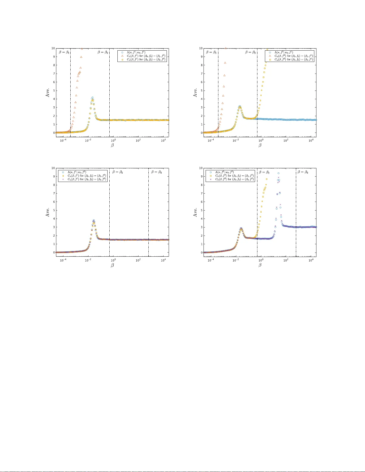
In trinsic regularization effect in Ba y esian nonlinear regression scaled by observ ed data Satoru T okuda, 1, 2, 3 , ∗ Kenji Nagata , 3 and Ma sato O k ada 3, 4 1 R ese ar ch Institute for Information T e chnolo gy, Kyushu U niversity, Kasuga, F ukuoka 816-8580 , Jap an 2 Mathematics for Ad vanc e d Materials – Op en Innovation L ab or atory, AIST, c/o A dvanc e d Institute for Materials R ese ar ch, T ohoku U niversity, Sendai, Miyagi, 980-8577, Jap an 3 Dep artment of Compl exity Scienc e and Engine ering, The University of T okyo, Kashiwa, Chib a 277-8561, Jap an 4 Center for Materials R ese ar ch by Information Inte gr ation, National Institut e for Mater ials Scienc e, Tsukub a, I b ar aki 305-0047, Jap an (Dated: D ecemb er 7, 2022) Occam’s razor is a guiding principle th at models should b e simple enough to describe observed data. While Ba yesia n mod el selection (BMS) em b o dies it by the intrinsic regularizatio n eff ect (IRE), how observed data scale the IRE has not b een fully understo o d. In the nonlinear regression with conditionally indep end ent observ ations, we show that th e IRE is scaled b y observ ations’ fineness, defined by the amount and quality of observed data. W e introd uce an observ able that quantifies the IRE, referred to as the Bay es sp ecific heat, inspired by th e correspondence betw een statis ti- cal inference and statistical ph ysics. W e derive its scaling relation to observ ations’ fin eness. W e demonstrate t hat the optimal mod el chosen by the BMS changes at critical v alues of observ ations’ fineness, accompanying the IRE’s v ariation. The changes are from choosing a coarse-grained mod el to a fine-grained one as observ ations’ fin eness increases. Our find ings expand an understanding of BMS’s typicalit y when observed d ata are insufficient. I. INTRO DUCTION T o descr ibe o bserved data by mathematical mo del is an impo r tant sta g e to understand the physics of the s ystem behind obser ved data. It is desired to build a mo del as simple as p ossible for caricaturing the es sential physics [1 – 5]. A simple mo del is a n equation or a function with fewer parameter s , which sometimes co rresp onds to an effective theory: a spe cial ca s e, an a pproximation, or a co arsening o f the more compr e he ns ive theory . Some attempts r elate the mo del simplicity to a kind of emer genc e as if microsco pic details a re a lmost negligible in macros copic phenomena fro m the viewp oint of information theor y [6 – 9]. They ar e also r elated to what mo del is simple enough for describing obser ved data well. In the context of sta tistics, some criteria for mo del s election, as highlig h ted by the Ak a ike and Bay esian information cr iteria (AIC a nd BIC), s upp or t selecting a simpler mo del as justifications of Oc c a m’s razor [10, 11]. Bay esian mo del selection (BMS) is utilized to c ho ose a mo del s imple enough to describ e the es s ent ial physics behind observed data [12 – 1 7]. Suppose that the gr ound truth that genera tes the obse r ved data is included in the list of candidate mo dels. There are se veral motiv a tions for employing the BMS. One is that the BMS is consistent [18, 19]. If the candidate mo dels ar e disjoin t, the mo del chosen by the BMS conv erges almost sure ly tow ar d the ground truth as o bserved data incr ease under mild conditions. Another is that the BMS automatically incorp or a tes Occam’s razor [18, 19]. If more than one candidate mo del can ex a ctly express the ground truth, the mo del c hosen b y the BMS conv er ges almost surely toward the simplest one with the fewest par ameters. W e s hould mention that our primary int erest in the BMS is choos ing the simplest mode l that describ es o bserved data w ell rather than verifying one ’s mo del (h yp othesis) based on the data. The simplest mo del for giv en data is sometimes consistent with the ground truth, but not necessarily . W e wan t to clar ify when and how the simplest mo del is the g round truth or other ca ndida tes. Occam’s ra z or in the BMS is em bo die d b y the intrinsic regulariz ation effect (IRE) that prefers simpler models to complex o nes as succe e ding to the BIC [11, 2 0, 21]. In the case of enough obs erved da ta , the singular lear ning theor y has rev ealed that the IRE is explicitly quan tified b y a birationa l inv aria nt , called the real log c anonical threshold (RLCT) [22 – 24]. How ever, how observed data sca le the IRE is still a c hallenging question. This question includes three issues. Fir s t, the RLCT do es not quantify the dep endence on the amount a nd qualit y of observed data. W e need the IRE’s scaling function that conv erge s toward the RLCT in the limit where they ar e sufficient. Second, the RLCT is not an observ able quantit y ca lculated from observed data but a q uantit y theoretically derived from the ground truth, which is prac tica lly unknown. While so me observ able quantities that co nv erg e tow ard the RLCT have bee n introduced [2 5 , 26], they do not explicitly represent the dep endence o n bo th the amo un t and q uality of observed ∗ s.tokuda.a96@m.kyush u- u.ac.jp 2 data. W e also need an observ a ble counterpart o f the sc a ling function. Third, how the IRE affects the BMS in the case of insufficien t observed data has yet to b e fully understo o d. While the BMS is c o nsistent, the mo del chosen by the BMS is not necessa rily the gro und truth if observed data a r e insufficient. W e also need to explain the t ypicality of the BMS for insufficient data by using the scaling function. Here we address these is s ues in the context of the no nlinear regres s ion with conditiona lly indep endent observ ations, which is a prototypical setup in mathematical mo deling. T o quantify the IRE, we in tro duce an observ able quantit y , referred to as the Bayes sp e c ific heat, inspired by the mathematical equiv alence b etw een statistica l inference and statistical physics [2 1, 27 – 2 9]. W e derive its finite-s ize scaling re lation to observ a tio ns’ fineness, defined by the amount and quality of observed data. W e show the cor resp ondence of the scaling function to the RLCT. W e demonstra te that the mo del chosen b y the BMS changes at critical v a lues of observ a tions’ fineness, affected by v ariatio n in the scaling function. W e also find that the changes a r e fro m choo sing a coarse - grained mo del to the fine-grained g round truth as o bserv ations ’ fineness increases. Our findings c o rresp ond to a typical b ehavior o f the BMS with a v a riation of obs erved data fr o m insufficient to sufficient, expanding an under standing of the BMS’s c o nsistency . II. ST A TISTICA L ENSEMBLE OF NONLINEAR REGRESSION W e star t b y defining a statistic al ensemble o f nonlinear reg ression. Let us consider obse rving conditionally indep en- dent r andom v a riables D n := { x i , Y i } n i =1 for x i = x i − 1 + L/ ( n − 1), where x 1 , x n , a nd L := x n − x 1 > 0 ar e fixed. W e assume that Y i ∼ N ( f ( x i ; w ) , β − 1 ), where f , w , and β − 1 > 0 are res pectively reg ression mo del, its parameter s et, and v ariance of o bserv ation no ise as an e mbo diment of the q uality of observed data. Here w e define obse r v ations’ fineness κ := nβ , whic h is a key quantit y of scaling relations as describ ed la ter. Since w and f are unknown and s ho uld b e estimated fro m D n , we treat them a s rando m elemen ts sub ject to the po sterior proba bilit y distribution p ( w, f | D n , β , µ ) ∝ exp  − κ 2 E n ( w ; f ) − κµF n ( β , f )  p ( w | f ) p ( f ) , (1) where E n ( w ; f ) := 1 n n X i =1 ( Y i − f ( x i ; w )) 2 (2) is the mea n squa r e error, F n ( β , f ) := − 1 κ log Z exp  − κ 2 E n ( w ; f )  p ( w | f ) dw (3) is the Bay es free energy , µ ≥ 0 is an auxiliar y v a riable, p ( w | f ) is an arbitrary prior probability distribution of w ∈ W ⊂ R d , and p ( f ) is that of f ∈ { f K } . If µ = 1, Eq. (1) is derived from Bayes’ theo rem. Throughout this study , w e consider the case µ → ∞ , which corr e spo nds to the empir ical Bayes approach, i.e., f is chosen by minimizing F n ( β , f ) at a given β as the BMS [20, 3 0, 31]. Note that the BIC a nd its generalized version are derived by approximating F n ( β , f ) [11, 25]. While β is given in E q . (1), if β is unknown, it ca n also b e estimated by minimizing κF n ( β , f ) − n (log β − log 2 π ) / 2 [32]. The ov erall setup is the basics o f our analys es in the following sections to cla rify the BMS transitions from choosing a coarse-g rained mo del to the fine-g rained gr ound truth as κ increa s es. II I. BA YES SPECIFIC HEA T W e in tro duce a key quantit y that c hara cterizes the macr ostates in the statistical ensem ble of nonlinear reg ression, which is defined as the fluctuation of E n ( w ; f ) at a certain pa ir of β and f with a g iven D n : C n ( β , f ) =  κ 2  2  h E n ( w ; f ) 2 i − h E n ( w ; f ) i 2  , (4) where h· · · i := R ( · · · ) p ( w | β , f , D n ) dw denotes the a verage over a ll micr ostates of w sub ject to p ( w | β , f , D n ) ∝ exp( − κE n ( w ; f ) / 2) p ( w | f ). Note that Eq. (4) is derived from a mor e gene r al definition of such a quant ity in statistical inference, c a lled the Bay es sp ecific heat (see App endix A). W e s hould men tion that C n ( β , f ) is an observ a ble that quantifies the IRE as ex plained in the next s ection. This q ua nt ity plays an imp ortant r ole in explaining the mec hanism of the BMS transitions in terms o f the IRE. 3 IV. FINITE-SIZE SCALING RELA TIONS W e hereafter consider the case that Y i ∼ N ( f 0 ( x i ; w 0 ) , β − 1 0 ), where f = f 0 , w = w 0 and β = β 0 are the ground truths such that p ( w 0 | f 0 ) > 0 is satisfied. The BMS dep ends on the set D n of n random v aria bles since it is carried out by minimizing F n ( β , f ), which is a function of D n . Bes ides, F n ( β , f ) dep ends on b oth D n and β ra ther than o n κ (see Eqs . (2) and (3)). T o clarify the typicalit y of BMS transitions, not dep ending on the realiza tion of D n but on κ , we take the limit where κ and L are fixe d, whereas n → ∞ . W e derive the finite-size sca ling relation F n ( β , f ) = F ( κ, f ; w 0 , f 0 ) + R n 2 nβ 0 (5) with the scaling function F ( κ, f ; w 0 , f 0 ) : = − 1 κ log Z exp  − κ 2 E ( w ; f , w 0 , f 0 )  p ( w | f ) dw (6) and the energ y function E ( w ; f , w 0 , f 0 ) := 1 L Z x n x 1 ( f 0 ( x ; w 0 ) − f ( x ; w )) 2 dx, (7) where R n is a random v aria ble sub ject to the chi-square distribution with n degr ee of freedom (see App endix B). Note that F n ( β , f ) is self-av er aging, i.e., F n ( β , f ) = [ F n ( β , f )] holds as n → ∞ , where [ · · · ] := R ( · · · ) Q n i =1 p ( y i | x i , w 0 , β 0 , f 0 ) dy i denotes the av erage o ver all r e a lizations of D n , which are sub ject to p ( y i | x i , w 0 , β 0 , f 0 ) := N ( f 0 ( x i ; w 0 ) , β − 1 0 ). Since R n / (2 nβ 0 ) is indep endent of f , f minimizing F ( κ, f ; w 0 , f 0 ) is e q ual to f minimizing F n ( β , f ) at κ consisting o f a certain pair of β and sufficiently large n . Under the condition β = β 0 , cor resp onding to the Nishimo ri line [33, 3 4], F ( κ, f ; w 0 , f 0 ) ena bles us to assess the typical b ehavior of statistica l ensemble at a certa in κ = nβ 0 , whic h is indep endent o f the rea lization of D n . Ba s ed on this typicality , we demonstra te that f minimizing F ( κ, f ; w 0 , f 0 ) at any κ is not necessa rily f 0 in the next section. The demonstration c la rifies the t ypicality of BMS transitions, independent of the realiza tions of D n , fro m cho o sing a co arse-g rained mo del to the fine- grained gr ound truth as κ increases . W e are interested in expla ining the mechanism of BMS tr ansitions in ter ms of the IRE. T o expla in the mechanism formally , in the a bove limit wher e κ a nd L ar e fixed, wher eas n → ∞ , we als o derive the finite-size scaling relation C n ( β , f ) = Λ ( κ, f ; w 0 , f 0 ) + O p  max  1 log κ , β β 0 , 1 n √ β 0  (8) with the scaling function Λ( κ, f ; w 0 , f 0 ) : =  κ 2  2  h E ( w ; f , w 0 , f 0 ) 2 i − h E ( w ; f , w 0 , f 0 ) i 2  , (9) where h· · · i conv erges to the a verage ov er p ( w | β , f , D n ) ∝ exp( − κE ( w ; f , w 0 , f 0 ) / 2) p ( w | f ) in the limit we consider (se e App endix C). F r om E q. (8), we find that C n ( β , f ) is an obse rv able co un terpart of Λ( κ, f ; w 0 , f 0 ) in the limit we co nsider. Note that C n ( β , f ) is conditio nally self-averaging, i.e., C n ( β , f ) = [ C n ( β , f )] holds a s n → ∞ if β = O ( β 0 / lo g n ). Thus, C n ( β , f ) is not necessarily se lf-av er aging under the condition β = β 0 , i.e., C n ( β 0 , f ) = Λ( nβ 0 , f ; w 0 , f 0 ) + O p (1) holds. W e a ssess the finite- s ize effect on some particula r ex a mples to v a lidate that the fluctua tion term O p  max  (log κ ) − 1 , β /β 0 , ( n √ β 0 ) − 1  is neglig ible at a ny β in some situations (see App endix D). W e also find that Λ( κ, f ; w 0 , f 0 ) is a quantification of the IRE in the limit we consider fro m the consider ation below. There is a junction b etw een Eq. (9) and the sing ular lear ning theory [22 – 25, 35, 36]. While the setup is based on independent and iden tically distributed obser v ations as n → ∞ in the related study [37], our setup is based on conditionally indep endent observ ations in the limit w he r e κ and L are fixed, wher eas n → ∞ . Our setup is a natura l extension, whe r e the limits of F ( κ, f ; w 0 , f 0 ) and Λ( κ, f ; w 0 , f 0 ) as κ → ∞ conv erge to the related study’s result. An y direct counterparts of C n ( β , f ) and Λ( κ, f ; w 0 , f 0 ) hav e not b e e n defined in the singular learning theory , while Eq. (8) is related to W a tanab e’s corollar y [25] (see App endices A and C). Thanks to this relation, the limit of Λ ( κ, f ; w 0 , f 0 ) as κ → ∞ is re g arded as the RLCT, which c haracter izes the IRE as the co efficient o f a leading term in the asymptotic expansion of F n ( β , f ) a s n → ∞ [22 – 24] (see Eq. (C23)). Namely , Λ( κ, f ; w 0 , f 0 ) quant ifies the IRE not only in the limit n → ∞ but also in the limit wher e κ and L are fixed, whereas n → ∞ . The limit Λ( κ, f ; w 0 , f 0 ) → dim ( w ) / 2 also holds as κ → ∞ if p ( w | D n , β , f ) is reg ular, wher e the BIC is justified [1 1, 25]. Based on these corresp ondences, we demonstr ate how the IRE is scaled by κ and how it affects the B MS transitions in the next section. 4 V. INTRINSIC REGULARIZA TION EFFECT SCA LED BY OBSER VED DA T A W e demonstr ate the BMS transitio ns from choos ing a coar s e-grained model to the fine-gr ained ground truth, affected by v a riation in the IRE, as κ increases. As a simple example, we n umerically demonstra te that f ∈ { f 0 , f 1 , f 2 } minimizing F ( κ, f ; w 0 , f 0 ) at a n y κ is not necess arily f 0 ∈ { f 0 , f 1 , f 2 } by using a nonlinear reg ression mo del with K Gaussian co mpo ne nts: f K ( x ; w ) = K X k =1 a k exp  − b k 2 ( x − c k ) 2  (10) for K ≥ 1 , where w := { a k , b k , c k } K k =1 is the parameter set. This mo del is regar ded as a kind of radial basis function net works [38]. Note that we define f 0 ( x ; w ) = 0, where w is a n empty set. W e also derive the analytic expression o f E ( w ; f , w 0 , f 0 ) for this f K (see App endix D). Let us consider a physic al in ter pretation of the statistic al ensemble of nonlinear regress ion with f K as an analogy . Based o n the ma thematical equiv alence be tw een statistical inference and statistical physics, the micr ostate w with the p article numb er K sub ject to p ( w, f | D n , β , µ ) is interpreted as a gr and c anonic al ensemble co nditioned by β as the inverse temp er atu r e , n as the volume , and µ a s the chemic al p otential . In the same manner, w sub ject to p ( w | β , D n , f ) is in terpreted as a c anonic al ensemble , where we a ssume p ( w, f | D n , β , µ ) = p ( w | D n , β , f ) p ( f | D n , β , µ ) to derive Eq.(1). Since b oth statistica l ensembles ar e als o conditioned b y the qu enche d disor der D n , w e discuss the typical macr ostate by mea ns of the tw o av er ages h· · · i and [ · · · ]. F or this purp ose, F ( κ, f ; w 0 , f 0 ) and Λ( κ, f ; w 0 , f 0 ) are reasona ble in the limit where κ and L are fixed, whereas n → ∞ . It should b e emphasiz e d that we do es not co nsider the thermo dynamic limit , i.e., the limit where K /n is fixed, whereas K → ∞ a nd n → ∞ . W e p erfor med an Mon te Ca r lo (MC) sim ulations by using pa rallel temp ering based on the Metrop olis crite- rion [39, 40]. The v a riable κ was discr etized as 400 p oints consis ting of κ = 0 and 39 9 lo garithmically spaced po int s in the interv al [1 0 − 8 , 10 12 ]. W e set the prior probability distribution as p ( w | f K ) = Q K k =1 exp( − a k / 10 − b k / 10 − c 2 k / 50) / (50 0 √ 2 π ). W e sim ulated p ( w | D n , β , f ) ∝ exp ( − κE n ( w ; f ) / 2) p ( w | f ) with a realization of D n to calculate F n ( β , f ) in the same manner a s in our previous work [32]. W e als o simulated p ( w | D n , β , f ) ∝ exp( − κE ( w ; f , w 0 , f 0 ) / 2) p ( w | f ) to calculate F ( κ, f ; w 0 , f 0 ) and Λ( κ, f ; w 0 , f 0 ) at each p oint of κ > 0 in the manner of Bridge sampling [41, 42]. In all the MC simulations, the total MC sweeps w ere 100,0 00 after the burn- in. The er ror bars o f F ( κ, f ; w 0 , f 0 ) and Λ ( κ, f ; w 0 , f 0 ) were calculated by b o otstrap r e s ampling. W e consider tw o c a ses to simulate the discov ery pro cess of the gross and fine str uc tur es in o bs erved data. One is the deg e ne r ate case that is defined as f 0 = f 1 with w 0 = { 10 , 10 , 0 } (Fig. 1a). Another is the splitting case tha t is defined as f 0 = f 2 with w 0 = { 5 , 10 , ( − 1) k × 0 . 25 } 2 k =1 , whic h makes tw o Gaussian comp onents str ongly overlapping (Fig. 1e). In each case, a realiza tion of D n for n = 10 1 is o btained in the presence of obser v ation noise at a certain β 0 . If β 0 is small e no ugh, f minimizing F n ( β , f ) in both cas es a re f 0 , whic h is not co nsistent with f 0 (Figs. 1b and 1f ). If β 0 is larg e to some extent, f minimizing F n ( β , f ) in b oth c a ses are f 1 , which is consistent/inconsistent with f 0 in the degenerate/splitting case (Figs. 1c and 1g). If β 0 is large e nough, f minimizing F n ( β , f ) in the splitting case is f 2 , which is consistent with f 0 (Fig. 1h). They s how that the optimal model chosen by the BMS is not alwa ys co nsistent with the ground truth and imply the t ypical behavior that the optimal model changes a t some critical v alues of obs erv ations’ fineness (rather than mag nitude of o bs erv ation noise); F or to o ro ugh observ ations , the optimal mo del just describ es a ”non-s tructure”. F o r rather r o ugh observ atio ns, the optimal model describ es a ” gross structure”. F or fine obs e rv ations, the optimal mo del des c rib es a ”fine structure”. T o elucidate our implication, we calculate F ( κ, f ; w 0 , f 0 ) and Λ( κ, f ; w 0 , f 0 ) on the Nishimori line κ = nβ 0 for the ab ov e t wo c ases. In b oth cas es ab ov e, the o ptimal mo del f minimizing F ( κ, f ; w 0 , f 0 ) c hanges from f 0 to f 1 around κ = κ c1 (Figs. 2a and 2c), while Λ( κ, f 1 ; w 0 , f 0 ) has a p eak a round κ = κ c1 (Figs. 2b and 2 d). Λ( κ, f 1 ; w 0 , f 0 ) is fa ir ly c onsistent with 0 and 1 . 5 at κ ≪ κ c1 and κ ≫ κ c1 , resp ectively (Fig. 2b) . Corresp onding changes in p ( w | D n , β , f 1 ) are also shown (Fig. 3). While p ( w | D n , β , f 1 ) at κ = κ 1 (Fig. 3a-3c) is fairly consistent with p ( w | f 1 ), p ( w | D n , β , f 1 ) at κ = κ 2 is sufficiently a pproximated by a Gaussian distributio n whose mean is w 0 (Figs. 3g-3i). p ( w | D n , β , f 1 ) at κ = κ c1 represents the intermediate state (Figs. 3d- 3f ) betw een these t wo states. Only in the splitting case, the optimal f minimizing F ( κ, f ; w 0 , f 0 ) changes from f 1 to f 2 around κ = κ c2 (Fig. 2c), while Λ( κ, f 1 ; w 0 , f 0 ) has a peak ar ound κ = κ c2 (Fig. 2 d). Λ( κ, f 2 ; w 0 , f 0 ) is fairly consistent with 1 . 5 and 3 at κ c1 ≪ κ ≪ κ c2 and κ ≫ κ c2 , resp ectively (Fig. 2d). Corr esp o nding changes in p ( w | D n , β , f 2 ) are also shown (Fig. 4 ). While p ( w | D n , β , f 2 ) at κ = κ 2 is far from a Gaussian distribution (Fig. 4a-4c; see also Appendix D), p ( w | D n , β , f 2 ) at κ = κ 3 is sufficiently a pproximated b y a bimo dal Ga ussian dis tribution whose mo des ar e symmetric (Fig. 4g- 4i). p ( w | D n , β , f 2 ) at κ = κ c2 represents the intermediate state (Fig. 4d-4f ) b etw een these t wo s ta tes. W e extend the inv estigation to the c a se that is defined as f 0 = f 2 with w 0 = { 5 , 10 , ( − 1) k × δ } 2 k =1 for 0 ≤ δ ≤ 2, where δ = 0 and δ = 0 . 25 r esp ectively corr e spo nd to the degenerate a nd splitting cases ab ov e. The phase diagr am 5 shows that there are three phases describ e d by κ and δ (Fig. 5 ). Three phases ar e bounded b y tw o ridge lines of Λ( κ, f 2 ; w 0 , f 2 ), where these lines merge in δ & 0 . 8. In other words, there is only tw o phases in δ & 0 . 8, while there are three phases 0 < δ . 0 . 8. Note that δ = 0 is a spe c ial case since the case of f 0 = f 2 with w 0 = { 5 , 10 , 0 } 2 k =1 is ident ified with the case of f 0 = f 1 with w 0 = { 1 0 , 10 , 0 } (see Appendix D). The optimal mo del f minimizing F ( κ, f ; w 0 , f 0 ) also changes ar ound the phase b ou ndaries . This corr e s po ndence enables us to interpret three phases as a ” non-structure” , a ”gro s s structur e”, and a ”fine str uc tur e”. Note that the r e g ion in the ”non-structure” pha se, whereas the optimal mo del is f = f 1 , cor resp onds to intermediate state, suc h as shown in Figs. 3d-3f. VI. DISCUSSIONS Our results clearly s how that the optima l mo del chosen by the BMS is not alwa ys consistent with the ground truth but depends o n observ ations’ fineness . The discovery pro cess o f the g ross and fine structur es s hows the c hang es in the optimal model at critical v alues of observ ations’ fineness, accompanying the v ariation in the IRE. Our r esults can also b e understo o d from another v iewpo int . An effectiv e model is not necessa r y to b e consistent with the optimal mo del for describing observed data since it is deduced from the or iginal theo ry independent of the data. If o ne is more confident o f an effective model than observed data, what mo del is optimal fo r observed data is replaced by what a mount a nd quality o f obser ved data are required to v alidate the model. Our results show that critical v alues of obse r v ations’ finenes s ar e re quired to do so . F rom this po in t, these v alues can b e rega rded as kinds of limits on an indire ct measur ement , i.e., parameter estimation of the effectiv e mo del. ACKNO WLEDGMENTS The a uthors are grateful to Chihiro H. Nak a jima, K o ji Hukushima, Ko uki Y onag a, Masayuki Ohzeki, Shotaro Ak aho, Sumio W atanab e, T omoyuki Obuchi a nd Y oshiyuki K abashima for v alua ble discuss ions. S.T. was supp orted by JSPS KAKE NHI (No. JP20K 19889 ). M.O. was suppor ted by JST CREST (No. JPMJCR17 6 1), JSP S K AKENHI (No. 25 12000 9), the ”Materia ls Research by Information Integration” Initiative (MI2 I) pro ject o f the Supp ort Progr am for Starting Up Innov a tio n Hub from the Japan Science and T echnology Agency (JST), and the Council fo r Science, T echnology and Innov a tion (CSTI), Cros s-ministerial Strategic I nnov ation Pr omotion Prog ram (SIP), ”Structural Materials for Inno v ation” (F unding ag ency: JST). App endix A: Defini tion of Bay e s sp ecific heat Here, we der ive Eq. (4 ) from a broader p ers p ective of statistical inference including our setup. W e star t by int ro ducing the conditional pr obability de ns it y p ( w | D n , ˜ β , β , f ) : = 1 ˜ Z n ( ˜ β , β , f ) exp − n ˜ β 2 L n ( w ; β , f ) ! p ( w | f ) (A1) with ˜ β ≥ 0 b eing the inverse temp er atur e [23], the empirical lo g loss function L n ( w ; β , f ) : = − 1 n n X i =1 log p ( Y i | x i , w , β , f ) (A2) and the pa rtition function ˜ Z n ( ˜ β , β , f ) : = Z exp − n ˜ β 2 L n ( w ; β , f ) ! p ( w | f ) dw. (A3) Note that Eq . (A1) for ˜ β = 1 is just B ayes’ theorem, where p ( w | D n , 1 , β , f ) and ˜ Z n (1 , β , f ) are the p osterior distribution and marg inal likelihoo d, resp e ctively . If ˜ β → ∞ a nd p ( ˆ w | f ) > 0, then p ( w | D n , ˜ β , β , f ) co nv erg es to δ ( w − ˆ w ), wher e ˆ w is the maximum likelihoo d es timator [23]. Notably , p ( w | D n , ˜ β , β , f ) = p ( w | f ) holds for ˜ β = 0. Here, we define the specific heat ˜ C n ( ˜ β , β , f ) : = ∂ h nL n ( w ; β , f ) i ˜ β ∂ ˜ β − 1 = ˜ β 2 ˜ I n ( ˜ β ; β , f ) (A4) 6 with the Fisher information ˜ I n ( ˜ β ; β , f ) : = *  ∂ ∂ ˜ β log p ( w | D n , ˜ β , β , f )  2 + ˜ β = h ( nL n ( w ; β , f )) 2 i ˜ β − h nL n ( w ; β , f ) i 2 ˜ β , (A5) where the av erage h· · · i ˜ β := R ( · · · ) p ( w | D n , ˜ β , β , f ) dw . Consider ing the co nnection betw een statistical inference and statistical physics, h nL n ( w ; β , f ) i ˜ β is the internal energ y and ˜ F n ( ˜ β , β , f ) : = − 1 ˜ β log ˜ Z n ( ˜ β , β , f ) . (A6) is the fre e energ y . Then, we also obtain the relation ˜ C n ( ˜ β , β , f ) = − ˜ β 2 ∂ 2 ( ˜ β ˜ F n ) ∂ ˜ β 2 (A7) as in s tatistical physics. As the Bay es free energ y is defined by ˜ F n (1 , β , f ), we define the Bayes sp ecific heat as ˜ C n (1 , β , f ), where this definition c an be applied not only to L n ( w ; β , f ) in the no nlinear regressio n but als o to empirical log loss functions o f any other sta tistical inference setups without lo ss of genera lity . W e should compare the Bayes spec ific heat, esp ecially in the form o f Eq. (A7) , with the learning capacity [4 3], whic h is defined by the second der iv ative of the Bay es free energ y with resp ect to n as an a ppr oximation of the se c ond-order- finite differenc e . Notably , the Bay es sp ecific hea t and the lea rning capacity are different, as ˜ β and n are different. How ever, they a ls o hav e similar ities. W e show their similarities and differences in App endix C. Now, we consider the sp ecifics of our setup, i.e., the relation L n ( w ; β , f ) = β 2 E n ( w ; f ) − 1 2 log β 2 π . (A8) Then, we obtain the scaling relations ˜ C n ( ˜ β , β , f ) = C n ( ˜ β β , f ) and ˜ I n ( ˜ β ; β , f ) = I n ( ˜ β β ; f ), where the scaling functions are C n ( ˜ β β , f ) : = ( ˜ β β ) 2 I n ( ˜ β β ; f ) (A9) and I n ( ˜ β β ; f ) : = h ( nE n ( w ; f )) 2 i ˜ β − h nE n ( w ; f ) i 2 ˜ β . (A10) Now, we take ˜ β = 1, i.e ˜ β β = β , and then obtain C n ( β , f ) in the form of Eq. (4) as the Bayes sp ecific hea t. App endix B: Deriv ation of scali ng relation on Bay e s free e nergy Here, we show an outline of the deriv ation of Eqs. (5) and (6). By cons idering the no ise additivity , we divided Y i int o the signal and noise, i.e., Y i = f 0 ( x i ; w 0 ) + N i , (B1) where N i ∼ N (0 , β − 1 0 ). Then, we obtained nE n ( w ; f ) = X i s i ( w ; f ) 2 + 2 X i s i ( w ; f ) N i + R n β 0 , (B2) where s i ( w ; f ) := f 0 ( x i ; w 0 ) − f ( x i ; w ) a nd R n := β 0 P i N 2 i . By using Jensen’s inequality , " − lo g Z exp − β 2 X i s i ( w ; f ) 2 + 2 X i s i ( w ; f ) N i !! p ( w | f ) dw # ≥ − log Z exp − β 2 X i s i ( w ; f ) 2 ! p ( w | f ) dw (B3) holds, where the equality holds when P i s i ( w ; f ) N i = 0, which is asymptotically satisfied for n → ∞ . Note that 1 n X i s i ( w ; f ) 2 = E ( w ; f , w 0 , f 0 ) (B4) also holds as n → ∞ . Based on these asymptotic b ehaviors, Eqs. (5) and (6) were o btained. 7 App endix C: Deriv ation and v alidation of scali ng rel ation on Bay e s sp ecific heat W e show the deriv ation of Eqs. (8) and (9) in more detail. W e start from a broader p e rsp ective o f statistical inference including our setup. The asymptotic behaviour of the free ener gy has b een obtained [23]: ˜ β ˜ F n ( ˜ β , β , f ) = n ˜ β L n ( w ′ 0 ; β , f ) + λ log n ˜ β + ( m − 1) log lo g n ˜ β + O p ( ˜ β ) (C1) as n → ∞ , where w ′ 0 is w that minimizes the Kullback-Leibler dis ta nce fro m p ( y | x, w 0 , β 0 , f 0 ) to p ( y | x, w, β , f ), λ > 0 is a rational num b er ca lled the real log ca nonical threshold, and m ≥ 1 is a natural num b er. Note that w ′ 0 = w 0 holds if β = β 0 and f = f 0 . By following Eqs. (A7) and (C1), w e obtain ˜ C n ( ˜ β , β , f ) = λ − ( m − 1)  1 log n ˜ β + 1 (log n ˜ β ) 2  + o p  ˜ β 2  (C2) as n → ∞ . If w e tak e ˜ β → ∞ , then ˜ C n ( ˜ β , β , f ) = λ + o p  ˜ β 2  holds; the quan tit y ˜ C n ( ˜ β , β , f ) is not necessar ily self-av eraging . The r elation ˜ C n ( ˜ β , β , f ) = λ holds a s n → ∞ if ˜ β = O (1 / log n ), which corresp onds to the condition shown in W atanab e’s co rollar y [25]: h nL n ( w ; β , f ) i ˜ β 1 − h nL n ( w ; β , f ) i ˜ β 2 ˜ β − 1 1 − ˜ β − 1 2 = λ + O p  1 √ log n  (C3) hold for ˜ β 1 = O (1 / log n ) a nd ˜ β 2 = O (1 / log n ), where ˜ β 1 and ˜ β 2 are pos itiv e v a riables. The r efore, it is recertified that ˜ C n ( ˜ β , β , f ) = λ holds for n → ∞ if ˜ β = O (1 / log n ), where h nL n ( w ; β , f ) i ˜ β 1 − h nL n ( w ; β , f ) i ˜ β 2 ˜ β − 1 1 − ˜ β − 1 2 = ˜ C n ( ˜ β , β , f ) (C4) hold a s ˜ β 1 → ˜ β and ˜ β 2 → ˜ β . Here, we mention that the expectation of the learning capa cit y over realizations a lso conv er ges to λ as n → ∞ [43]. Howev er , it has not pr ov en that the lear ning capacity as a random v ar iable conv erges tow ar d λ as n → ∞ . The lea r ning capacity as a random v a riable is not applicable for the scaling ana ly sis that provides Eq. (C2). It do e s not a lso provide Eqs. (8) a nd (9) in the limit where κ and L ar e fixed, whereas n → ∞ . Now, we consider the sp ecifics of our setup, i.e., the scaling relatio n C n ( ˜ β β , f ) = λ − ( m − 1)  1 log ˜ β κ + 1 (log ˜ β κ ) 2  + o p  ˜ β 2 β 2  , ( C5) where the corresp ondence of ( ˜ β , β ) a nd ˜ β β is co nsidered. Then, we obtain C n ( β , f ) = λ − ( m − 1)  1 log κ + 1 (log κ ) 2  + o p  β 2  (C6) for ˜ β = 1. W e als o ev alua te the term o p  β 2  more tightly . F ollowing Eqs. (2) a nd (B2), we obtain C n ( β , f ) =  β 2  2   * n X i =1 s i ( w ; f ) 2 ! 2 + − * n X i =1 s i ( w ; f ) 2 + 2   + V n ( β , f ) + ˜ V n ( β , f ) + W n ( β , f ) + ˜ W n ( β , f ) , (C7) where V n ( β , f ) : = β 2 X i 6 = j ( h s i ( w ; f ) s j ( w ; f ) i − h s i ( w ; f ) i h s j ( w ; f ) i ) N i N j , (C8) ˜ V n ( β , f ) : = β 2 n X i =1   s i ( w ; f ) 2  − h s i ( w ; f ) i 2  N 2 i , (C9) 8 W n ( β , f ) : = β 2 X i 6 = j  s i ( w ; f ) 2 s j ( w ; f )  −  s i ( w ; f ) 2  h s j ( w ; f ) i  N j , (C10) and ˜ W n ( β , f ) := β 2 n X i =1  s i ( w ; f ) 3  −  s i ( w ; f ) 2  h s i ( w ; f ) i  N i . (C11) W e ev alua te the o rder of each term in E q. (C7) in the limit where κ a nd L ar e fixed, wherea s n → ∞ . First, w e obtain  β 2  2   * n X i =1 s i ( w ; f ) 2 ! 2 + − * n X i =1 s i ( w ; f ) 2 + 2   = Λ( κ, f ; w 0 , f 0 ) (C12) in the limit that w e consider . Second, we ev aluate the order o f V n ( β , f ) as n → ∞ . Now, we o bta in [ V n ( β , f )] = 0 (C13) as n → ∞ , such that [ h ( h s i ( w ; f ) s j ( w ; f ) i − h s i ( w ; f ) i h s j ( w ; f ) ii ) N i N j ] = ( h s i ( w ; f ) s j ( w ; f ) i − h s i ( w ; f ) i h s j ( w ; f ) i ) [ N i ][ N j ] (C14) is satisfied, where [ N i ] = 0. Then, we a lso obtain  V n ( β , f ) 2  − [ V n ( β , f )] 2 = β 4 β 2 0 X i 6 = j ( h s i ( w ; f ) s j ( w ; f ) i − h s i ( w ; f ) i h s j ( w ; f ) i ) 2 = O  β 2 β 2 0  (C15) as n → ∞ , such that h ( h s i ( w ; f ) s j ( w ; f ) i − h s i ( w ; f ) i h s j ( w ; f ) i ) 2 N 2 i N 2 j i = ( h s i ( w ; f ) s j ( w ; f ) i − h s i ( w ; f ) i h s j ( w ; f ) i ) 2 [ N 2 i ][ N 2 j ] (C16) and [( h s i ( w ; f ) s j ( w ; f ) i − h s i ( w ; f ) i h s j ( w ; f ) i ) ( h s k ( w ; f ) s l ( w ; f ) i − h s k ( w ; f ) i h s l ( w ; f ) i ) N i N j N k N l ] = ( h s i ( w ; f ) s j ( w ; f ) i − h s i ( w ; f ) i h s j ( w ; f ) i ) ( h s k ( w ; f ) s l ( w ; f ) i − h s k ( w ; f ) i h s l ( w ; f ) i ) [ N i ][ N j ][ N k ][ N l ] (C17) are satisfied, where [ N i ] = 0, [ N 2 i ] = β − 1 0 , h s i ( w ; f ) i = O ( κ − 1 ) and h s i ( w ; f ) s j ( w ; f ) i = O ( κ − 1 ). In summar y , w e obtain V n ( β , f ) = [ V n ( β , f )] + O p  β β 0  = O p  β β 0  (C18) as n → ∞ . In the same wa y , we also obtain ˜ V n ( β , f ) = h ˜ V n ( β , f ) i + O p  β √ nβ 0  (C19) as n → ∞ with h ˜ V n ( β , f ) i = β 2 β 0 n X i =1   s i ( w ; f ) 2  − h s i ( w ; f ) i 2  = O  β β 0  , (C20) 9 where [ N 2 i ] = β − 1 0 ,  N 4 i  = 3 /β 2 0 , h s i ( w ; f ) i = O ( κ − 1 ) and  s i ( w ; f ) 2  = O ( κ − 1 ). This means that ˜ V n is self-averaging; i.e., ˜ V n = [ ˜ V n ] ≥ 0 holds as n → ∞ . F urthermo r e, w e also obtain W n ( β , f ) = O p  1 n √ β 0  , (C21) and ˜ W n ( β , f ) = O p  1 n 3 / 2 √ β 0  (C22) as n → ∞ , wher e [ N i ] = 0, [ N 2 i ] = β − 1 0 , [ W n ] = 0, [ ˜ W n ] = 0, h s i ( w ; f ) i = O ( κ − 1 ),  s i ( w ; f ) 2  = O ( κ − 1 ),  s i ( w ; f ) 2 s j ( w ; f )  = O  κ − 2  , and  s i ( w ; f ) 3  = O  κ − 2  . By consider ing the consistency b etw een Eq s. (C6) and (C7) with E qs. (C12) and (C18-C22), we obtain Eqs. (8) and (9), where Λ( κ, f ; w 0 , f 0 ) = λ as κ → ∞ is the real log canonical threshold. F r om this asymptotic behavior and Eq. (C1), it is fo und out that Λ( κ, f ; w 0 , f 0 ) and C n ( β , f ) repres en t the intrinsic regular ization effect in F n ( β , f ) as κ → ∞ : κF n ( β , f ) = nL n ( w ′ 0 ; β , f ) + λ log n + ( m − 1 ) log log n + n 2 log β 2 π + O p (1) , (C23) where ˜ F n (1 , β , f ) = κF n ( β , f ) − n (lo g β − log 2 π ) / 2 holds [3 2]. Here, we demonstrate the v alidity of Eqs. (8) and (9). By perfo rming the same simulation in Fig. 1 based on 100 differen t realizations of D n for n = 1 01 tak en fro m iden tical p ( y i | x i , w 0 , β 0 ), we c a lculate C n ( β , f ) for each realization. At any β , the exp e c tation of C n ( β , f 1 ) ov e r the realizations is fairly consis ten t with Λ( κ, f 1 ; w 0 , f 1 ) if β 0 = β 2 (Fig. A1 a), Λ ( κ, f 1 ; w 0 , f 2 ) (Fig. A1 c), and Λ( κ, f 2 ; w 0 , f 2 ) if β 0 = β 3 . The sta ndard devia tions of C n ( β , f ) for the realiza tions is small enoug h (Fig. A2 ); the quantit y C n ( β , f ) is considere d to be self-av er aging at an y β in these cases without the condition β = O ( β 0 / lo g n ). According to Eq. (8), these cas es mean that the exp ectation of C n ( β , f ) corresp onds to the average term Λ ( κ, f ; w 0 , f 0 ), wher e the standard devia tion of C n ( β , f ) corre spo nds to the fluctuation ter m of or der O p  max  (log κ ) − 1 , β /β 0 , ( n √ β 0 ) − 1  . Note that the standar d deviation o f C n ( β , f ) as the fluctuation ter m shows a dep endence on Λ( κ, f ; w 0 , f 0 ) (Fig. A2 ), which is not predicted by Eq. (8). In other cases, the expec tation of C n ( β , f ) is not consisten t with Λ( κ, f ; w 0 , f 0 ) at β & β 0 (Fig. A1 ); finite-size effects on C n ( β , f ) app ear at β & β 0 , where the ter m of o rder O p ( β /β 0 ) is dominant. According to Eq. (C7) with Eqs. (C18-C22), the exp ectation of C n ( β , f ) corresp onds to Λ( κ, f ; w 0 , f 0 ) + ˜ V n ( β , f ) a s n → ∞ , wher e the standard deviation of C n ( β , f ) corresp onds to V n ( β , f ) + W n ( β , f ) + ˜ W n ( β , f ) as n → ∞ . The expectations and standard devia tions of C n ( β , f ) ar e roughly pr op ortional to √ β if β is larg e enough (Fig. A3 ) a nd also show a rough depe ndence on β 2 0 . Note that C n ( β , f ) is considered to be self-av eraging for β = O ( β 0 / lo g n ) in all c ases. App endix D: Energy function of radial bas i s function netw ork Here, we derive the analytic expr ession of E ( w ; f , w 0 , f 0 ) for f , f 0 ∈ { f K } , wher e f K is defined as Eq. (1 0): E ( w ; f , w 0 , f 0 ) = H ( w 0 , w 0 ) − 2 H ( w 0 , w ) + H ( w , w ) (D1) with H ( w , w ′ ) : = 1 L K X j =1 K ′ X k =1 a j a ′ k s 2 b j + b ′ k exp − ( c j − c ′ k ) 2 2  b − 1 j + b ′− 1 k  ! ˜ H ( b j , c j , b ′ k , c ′ k ) (D2) for w ′ := { a ′ k , b ′ k , c ′ k } K ′ k =1 as K K ′ > 0 and H ( w , w ′ ) := 0 as K K ′ = 0, where ˜ H ( b j , c j , b ′ k , c ′ k ) : = √ π 2 erf r b j + b ′ k 2  x n − c j b j + c ′ k b ′ k b j + b ′ k  ! − √ π 2 erf r b j + b ′ k 2  x 1 − c j b j + c ′ k b ′ k b j + b ′ k  ! . (D3) Note that ˜ H ( b j , c j , b ′ k , c ′ k ) = √ π holds as x 1 → − ∞ and x n → ∞ . W e explain wh y p ( w | D n , β , f 2 ) at κ = κ 2 (Figs.4a-4 c) exhibits such a cor relation in the parameter s. Although the gr ound truth are f 0 = f 2 with w 0 = { 5 , 10 , ( − 1 ) k × 0 . 25 } 2 k =1 , here, we consider the ps eudo-gro und truth ˜ f 0 = f 1 with ˜ w 0 := { a ∗ , b ∗ , c ∗ } and the analytic set ˜ W 0 := { w | f ( x i ; w ) = ˜ f 0 ( x i ; ˜ w 0 ) } = ˜ W 01 ∪ ˜ W 02 ∪ ˜ W 03 (D4) 10 for w := { a k , b k , c k } 2 k =1 , where ˜ W 01 := { w | a k + a k ′ = a ∗ , b k = b k ′ = b ∗ , c k = c k ′ = c ∗ } , (D5) ˜ W 02 := { w | a k = a ∗ , a k ′ = 0 , b k = b ∗ , c k = c ∗ } , (D6) and ˜ W 03 :=  w | a k = a ∗ , b k = b ∗ , c k = c ∗ , exp  − b k ′ 2 ( x i − c k ′ ) 2  = 0  (D7) for i = 1 , · · · , n and k 6 = k ′ . Note that exp( − b k ′ ( x i − c k ′ ) 2 / 2) = 0 holds as b k ′ → ∞ or c k ′ → ± ∞ , where b k ′ 6 = 0 and c k ′ 6 = x i are necessary . Notably , E ( ˜ w ; f 2 , ˜ w 0 , ˜ f 0 ) = 0 holds for ∀ ˜ w ∈ ˜ W 0 ; i.e., p ( w | D n , β , f 2 ) can be re latively large around w = ˜ w for p ( w | f 2 ) > 0. The above scena r io o f the pseudo-g round truth corre s po nds to p ( w | D n , β , f 2 ) at κ = κ 2 (Figs. 4 a-4c); i.e., w ≃ ˜ w 0 is statistically optimal for f = f 2 at κ = κ 2 . This scena r io qualitatively holds at any κ c1 ≪ κ ≪ κ c2 , since Λ( κ, f 2 ; w 0 , f 2 ) is fairly consistent with 1 . 5(= Λ( κ, f 1 ; w 0 , f 2 )). No te that this result is from the situation where f 0 = f 2 ( x ; w 0 ) app ear s almos t as one Ga us sian component (Fig. 1e), where one can o nly capture a ”gross structure” depending on obs erv ations’ fineness. [1] N. D. Goldenfeld, L e ctur es on phase tr ansitions and the r enormalization gr oup (A ddison-W esley , 1992). [2] N. Goldenfeld and L. P . Kadanoff, Simple lessons from complexit y , Science 284 , 87 (1999). [3] R. W. Batterman, Asymptotics and the role of minimal mo d els, The British Journal for the Philosoph y of Science 53 , 21 (2002). [4] R. W. Batterman and C. C. Rice, Minimal mod el exp lanations, Philosophy of Science 81 , 349 (2014). [5] Y. Oono, The nonline ar world: Con c eptual analysis and phenomenolo gy (Sp ringer Science & Business Media, 2012). [6] E. P . H oel, L. Albantakis, and G. T ononi, Quantifying causal emergence shows that macro can b eat micro, Pro ceedings of the National Academy of Sciences 110 , 19790 (2013). [7] B. B. Mach ta, R. Chachra, M. K. T ranstru m , and J. P . Sethna, P arameter space compression underlies emergent theories and pred ictiv e mo dels, Science 342 , 604 (2013). [8] H. H. Mattingly , M. K. T ranstrum, M. C. Ab b ott, and B. B. Mach ta, Maximizing the information learned from fi nite d ata selects a simple model, Proceed in gs of the National Academy of Sciences 115 , 1760 (2018). [9] A. Gordon, A. Banerjee, M. Ko ch-Jan usz, and Z. R in gel, Relev ance in th e renormalization group and in information theory , Physica l Review Letters 126 , 24060 1 (2021). [10] H. Ak aike, A n ew lo ok at the statistical mo del identificatio n, IEEE t ran sactions on automatic con trol 19 , 716 (1974). [11] G. Sch warz et al. , Estimating the d imension of a mod el, Ann als of statistics 6 , 461 (1978). [12] R. T rotta, Ba yes in t h e sk y: Ba yesian inference and mod el selection in cosmolog y , Contemporary Physics 49 , 71 (2008). [13] R. P . Mann, Bay esian in ference for identifying interactio n rules in moving animal groups, PloS one 6 , e22827 (2011). [14] C. Mark, C. Metzner, L. Lautsc ham, P . L. Strissel, R. Strick, and B. F abry , Bay esian mo del selection for complex dynamic systems, Natu re communications 9 , 1 ( 2018). [15] J. A . V´ azquez, D. T ama yo, A. A . Sen, and I . Quiros, Bay esian model selection on scala r ε -field dark energy , Physical Review D 103 , 043506 (2021). [16] S. T okuda, S . S ou ma, K. S ega w a, T. T ak ahashi, Y. An do, T. Nak anishi, and T. Sato, U nv eiling q uasiparticle dyn amics of top ologica l insu lators through bay esian mo delling, Comm unications Physics 4 , 1 (2021). [17] S. T okuda, Y. Kaw achi, M. Sasaki, H. Arak aw a, K. Y amasaki, K. T erasak a, and S. Inagaki, Bay esian inference of ion velocit y d istribution function from laser-induced fluorescence spectra, Scientific Rep orts 11 , 1 (2021). [18] L. W asserman, Ba yesi an mo del selection and mo del av eraging, Journal of mathematical psychology 44 , 92 (2000). [19] J. O. Berger, L. R. P ericc hi, J. Gh osh, T. Samanta, F. De Santis, J. Berger, and L. Pericc h i, Ob jective bay esian metho ds for mo del selection: I ntroduction and comparison, Lecture Notes-Monograph Series , 135 (2001). [20] D. J. MacKay , Ba yesia n interpolation, Neural computation 4 , 415 (1992). [21] V. Balasubramanian, Statistical inference, o ccam’s razor, and statistical mechanics on the space of probability distribut ions, Neural computation 9 , 349 (1997). [22] S. W atanab e, Algebraic analysis for nonidentifiable learning mac hines, Neural Computation 13 , 899 (2001). [23] S. W atanab e, A lgebr aic ge ometry and statistic al le arning the ory , V ol. 25 (Cam bridge Universit y Press, 2009). [24] S. W atanab e, Mathematic al the ory of Bayesian statistics (CRC Press, 2018). [25] S. W atanab e, A widely applicable bay esian information criterion, Journal of Mac hine Learning Researc h 14 , 867 (2013). [26] S. T okuda, K . Nagata, and M. Ok ada, A numerical analysis of learning coefficient in radial basis fun ct ion netw ork, I PSJ Online T ransactions 7 , 20 (2014). [27] E. T. Jaynes, I nformation theory and statistical mechanics, Physical review 106 , 620 (1957). [28] E. T. Jaynes, Pr ob abili ty the ory: The lo gic of scienc e (Cambridge un ive rsity press, 2003). [29] L. Zdeb oro v´ a and F. K rzaka la, Statistical physics of inference: Thresholds and algorithms, Adv ances in Physic s 65 , 453 (2016). 11 [30] B. Efron and C. Morris, S tein’s estimation rule and its comp etitors—an empirical ba yes approach, Journal of the A merican Statistical Association 68 , 117 (1973). [31] H. Ak aike, Likeli ho od and th e bay es p rocedu re, in Sele cte d Pap ers of Hi r otugu Akaike (S pringer, 1998) pp. 309–33 2. [32] S. T okuda, K. Nagata, and M. Okada, S im ultaneous estimation of noise v ariance and num b er of p eaks in bay esian sp ectral deconv olution, Journal of th e Physical So ciet y of Japan 86 , 024001 (2017). [33] H. Nishimori, Exact results and critical prop erties of the ising mod el with comp eting interactions, Journal of Physics C: Solid S tate Physics 13 , 4071 (1980). [34] Y. Iba, The nishimori line and baye sian statistics, Journal of Ph ysics A: Mathematical and General 32 , 3875 (1999). [35] S. W atanab e, Equations of states in singular statistical estimation, Neural N etw orks 23 , 20 (2010). [36] S. W atanab e, Asymptotic equiv alence of ba yes cross va lidation and widely applicable informa tion criterion in singular learning theory , Journal of Mac hine Learning Researc h 11 , 3571 (2010). [37] S. W atanab e et al. , A limit theorem in singular regression problem, in Pr ob abi listic Appr o ach to Ge ometry (Mathematical Society of Japan, 2010) pp . 473–492. [38] D. BR OOMHEAD, Multiv ariable functional in terp olation and adaptive net works, Complex S ystems 2 , 321 ( 1988). [39] C. J. Geyer, Marko v chain monte carlo maximum lik elihoo d (I nterf ace F oundation of N orth America, 1991). [40] K. H ukushima and K. Nemoto, Exc hange monte carlo method and application to spin glass sim ulations, Journal of the Physica l Society of Japan 65 , 1604 (1996). [41] X.-L. Meng and W. H . W ong, Simulating ratios of normalizing constants via a simple identit y: a theoretical ex ploration, Statistica Sinica , 831 (1996). [42] A. Gelman and X.-L. Meng, Sim ulating normalizing constants: F rom importance sampling to bridge sampling to path sampling, Statistical science , 163 (1998). [43] C. H. LaMont and P . A. Wiggins, Corresp ondence betw een thermo dynamics and inference, Physical Review E 99 , 052140 (2019). 12 FIG. 1. Ground truth , observ ed data, and op t imal mod el chosen by Ba yesian model selection. It is demonstrated th at whic h mod el minimizes F n ( β , f ) for each realization of D n (blac k dots) with n = 101, f = f 0 ( x ; w ) (n o line), f = f 1 ( x ; w ) (red solid line), or f = f 2 ( x ; w ) (red dashed line) with tw o Gaussian comp onents (blue solid lines). F or the degenerate case that the ground truth is ( a ) f 0 = f 1 ( x ; w 0 ) with w 0 = { 10 , 10 , 0 } , the minimal mo d el is ( b ) f = f 0 at β 0 = κ 1 /n , ( c ) f = f 1 at β 0 = κ 2 /n , and ( d ) f = f 1 at β 0 = κ 3 /n . F or the splitting case th at th e ground trut h is ( e ) f 0 = f 2 ( x ; w 0 ) with w 0 = { 5 , 10 , ( − 1) k × 0 . 25 } 2 k =1 , the minimal mo del is ( f ) f = f 0 at β 0 = κ 1 /n , ( g ) f = f 1 at β 0 = κ 2 /n , and ( h ) f = f 2 at β 0 = κ 3 /n . 13 FIG. 2. Ba yesia n mod el selection and intrinsi c regularization effect scaled by observ ations’ fi neness. The inequalit y F ( κ, f 0 ; w 0 , f 0 ) < F ( κ, f 1 ; w 0 , f 0 ) holds for κ < κ c1 (region in ligh t blue), F ( κ, f 0 ; w 0 , f 0 ) > F ( κ, f 1 ; w 0 , f 0 ) holds for κ c1 < κ < κ c2 (region in light pink), and F ( κ, f 1 ; w 0 , f 0 ) > F ( κ, f 2 ; w 0 , f 0 ) holds for κ > κ c2 (region in light yel low ). ( a ) Log-log plot of F ( κ, f ; w 0 , f 1 ) for w 0 = { 10 , 10 , 0 } . In set sho ws that the Bay es factor exp( − κ ( F ( κ, f 2 ; w 0 , f 1 ) − F ( κ, f 1 ; w 0 , f 1 ))) < 1 holds for any κ . ( b ) S emi- log plot of Λ( κ, f ; w 0 , f 1 ) for w 0 = { 10 , 10 , 0 } and asymptote dim( w ) / 2 = 1 . 5 (b lac k dot- ted line). ( c ) Log-log p lot of F ( κ, f ; w 0 , f 2 ) for w 0 = { 5 , 10 , ( − 1) k × 0 . 25 } 2 k =1 . I nset shows that the Ba yes factor exp( − κ ( F ( κ, f 2 ; w 0 , f 2 ) − F ( κ, f 1 ; w 0 , f 2 ))) < 1 holds for κ < κ c2 , and exp( − κ ( F ( κ, f 2 ; w 0 , f 2 ) − F ( κ, f 1 ; w 0 , f 2 ))) > 1 holds for κ > κ c2 . ( d ) Semi-log plot of Λ( κ, f ; w 0 , f 2 ) for w 0 = { 5 , 10 , ( − 1) k × 0 . 25 } and asymptote dim( w ) / 2 = 3 (black dotted line). 14 FIG. 3. Change in the p osterior probability distribution from the p rior p robabilit y distribution depend ing on observ ations’ fineness. Histogram of the Monte Carlo sample from p ( w | D n , β , f 1 ) ∝ exp( − κE ( w ; f 1 , w 0 , f 1 ) / 2) p ( w | f 1 ) for w 0 = { 10 , 10 , 0 } at ( a - c ) κ = κ 1 , ( d - f ) κ = κ c1 , and ( g - i ) κ = κ 2 . Eac h ro w corresponds to a marginal distribution; ( a , d , g ) corresponds to p ( a 1 | D n , β , f 1 ), ( b , e , h ) corresponds to p ( b 1 | D n , β , f 1 ), and ( c , f , i ) corresp onds t o p ( c 1 | D n , β , f 1 ). Compare eac h histogram with the marginal d istribution of p ( w | f 1 ) (red dashed line). 15 FIG. 4. Change in the posterior p robabilit y distribution dep ending on observ ations’ fineness and u nderlying parameter corre- lations. Two-dimensional histogram of th e Mon te Carlo sample from p ( w | D n , β , f 2 ) ∝ exp( − κE ( w ; f 2 , w 0 , f 2 ) / 2) p ( w | f 2 ) for w 0 = { 5 , 10 , ( − 1) k × 0 . 25 } 2 k =1 at ( a - c ) κ = κ 2 , ( d - f ) κ = κ c2 , and ( g - i ) κ = κ 3 . Each ro w corresponds to a margi nal distribution; ( a , d , g ) corresponds to p ( a 1 , a 2 | D n , β , f 2 ), ( b , e , h ) corresp onds to p ( b 1 , b 2 | D n , β , f 2 ), and ( c , f , i ) corresp onds to p ( c 1 , c 2 | D n , β , f 2 ). 16 FIG. 5. Phase diagram with respect to observ ations’ fineness and ground truth of parameter. Semi-log p lot of th e peak p ositions of Λ( κ, f 2 ; w 0 , f 2 ) (black dashed and grey solid lines) for w 0 = { 5 , 10 , ( − 1) k × δ } 2 k =1 . The inequality F ( κ, f 0 ; w 0 , f 2 ) < F ( κ, f 1 ; w 0 , f 2 ) holds for κ < κ c1 ( δ ) (region in light blue), F ( κ, f 0 ; w 0 , f 2 ) > F ( κ, f 1 ; w 0 , f 2 ) holds for κ c1 ( δ ) < κ < κ c2 ( δ ) (region in light pink), and F ( κ, f 1 ; w 0 , f 2 ) > F ( κ, f 2 ; w 0 , f 2 ) holds for κ > κ c2 ( δ ) ( region in light yello w). 17 a b c d FIG. A1 . Finite-size effects on th e Ba yes sp ecific h eat. Semi-log plots of Λ( κ, f ; w 0 , f 0 ) (blue circles) and th e exp ectations of C n ( β , f ) ove r realizati ons of D n for β 0 = β 1 (red triangles), β 0 = β 2 (yello w squares) and β 0 = β 3 (purple crosses), where β = κ/n ( β 1 := κ 1 /n , β 2 := κ 2 /n , and β 3 := κ 3 /n ). F or the case that the ground truth is f 0 = f 1 with w 0 = { 10 , 10 , 0 } , ( a ) C n ( β , f 1 ) and ( b ) C n ( β , f 2 ) are resp ectively compared with Λ( κ, f 1 ; w 0 , f 1 ) and Λ( κ, f 2 ; w 0 , f 1 ) shown in Fig. 2b. F or th e case th at the ground tru th is f 0 = f 1 with w 0 = { 5 , 10 , ( − 1) k × 0 . 25 } 2 k =1 , ( c ) C n ( β , f 1 ) and ( d ) C n ( β , f 2 ) are respectively compared with Λ( κ, f 1 ; w 0 , f 2 ) and Λ( κ, f 2 ; w 0 , f 2 ) shown in Fig. 2d . 18 FIG. A2 . Fluctuation of th e Ba yes specific heat for real izations. Log-log plots of the standard deviation of C n ( β , f ) for realizations of D n for ( β 0 , f 0 ) = ( β 2 , f 1 ) (blue squares for f = f 1 ), ( β 0 , f 0 ) = ( β 2 , f 2 ) (red sq uares for f = f 1 ), and ( β 0 , f 0 ) = ( β 3 , f 2 ) (yello w crosses for f = f 1 and pu rple crosses for f = f 2 ), where each case corresponds to Fig. A1 . 19 a b c FIG. A 3 . Scaling analyses of the Ba yes sp ecific heat. Log-lo g p lots of the exp ectations (blue triangles for f 0 = f 1 and yel low squares for f 0 = f 2 ) of C n ( β , f ), subtracting Λ( κ, f ; w 0 , f 0 ) as the baseline, and the standard dev iations (red triangles for f 0 = f 1 and yello w squares for f 0 = f 2 ) of C n ( β , f ) ov er realizations of D n in the cases of ( a ) Fig. A1 a , ( b ) Fig. A1 b and ( c ) Fig. A1 d .