The Existence of Equilibrium Flows

In this paper, we establish conditions for the existence of an equilibrium in the equilibrium flow problem studied by Galichon et al. (2024). The problem nests several classical economic models such as bipartite matching models, hedonic pricing models, shortest-path and minimum-cost flow problems, and time-dependent routing problems.

💡 Research Summary

**
The paper revisits the “equilibrium flow” framework introduced by Galichon, Samuels, and Vernet (2022) and provides a rigorous existence theorem for equilibrium prices and flows under three structural assumptions. The model is defined on a finite directed network ((Z,A)) with a price vector (p\in\mathbb{R}^Z) and a family of continuous, increasing connection functions (G_{xy}:\mathbb{R}\to\mathbb{R}) for each arc (xy\in A). An external flow vector (q\in\mathbb{R}^Z) satisfies (\sum_{z}q_z=0) and represents net supply (positive) or demand (negative) at each node. Internal flows (\mu\in\mathbb{R}^A_{+}) must satisfy the mass‑balance equation (\nabla^{\top}\mu = q), where (\nabla) is the node‑arc incidence matrix.

An equilibrium outcome ((q,\mu,p)) is defined by three conditions: (i) mass balance, (ii) no positive rent on any arc, i.e. (p_x\ge G_{xy}(p_y)) for all (xy\in A), and (iii) complementary slackness, i.e. (\mu_{xy}>0) implies (p_x = G_{xy}(p_y)). These conditions capture a market‑like “zero‑profit” equilibrium.

The authors introduce three key assumptions:

1. Feasibility (Assumption 1). For any “retaining” set (B\subset Z) (no outgoing arcs), the total external flow satisfies (q(B)\ge0). This guarantees that a feasible internal flow (\mu) exists. Lemma 1 shows that this condition is equivalent to the existence of a non‑negative flow solving the balance equations, and it is precisely the condition appearing in Hall’s marriage theorem.

2. Technical Connectivity (Assumption 2). Every node either has positive external supply or can reach a node with positive supply via a directed path. This eliminates isolated nodes that could never carry flow, allowing the construction to focus on the relevant sub‑network.

3. No Profitable Cycles (Assumption 3). For any directed cycle ((x_0,\dots,x_k,x_0)) and any price level (p), we have (p > G_{x_0x_1}\circ G_{x_1x_2}\circ\cdots\circ G_{x_kx_0}(p)). This rules out “money‑pump” cycles that would generate infinite rent, ensuring that a consistent price vector can be assigned.

Under these assumptions, Theorem 1 asserts the existence of an equilibrium flow. The proof proceeds in two major steps:

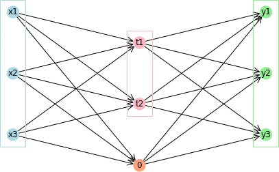
• Reduction to a Bipartite Matching Problem. Define source nodes (X={z:q_z<0}) and target nodes (Y={z:q_z>0}). For each pair ((x,y)) introduce the maximal connection function (\tilde G_{xy}(p_y)=\sup{G_{x_0x_1}\circ\cdots\circ G_{x_k y}(p_y)\mid\text{paths }x\to y}). The original equilibrium flow problem is shown (Lemma 2) to be equivalent to an “imperfectly transferable utility” bipartite matching problem ((X,Y,\tilde G)) with the same external flow vector. This bridges the problem to classical combinatorial optimization.

• Construction of Prices and Flows. Starting from an equilibrium of the bipartite matching (which exists by Hall’s condition, Lemma 4), the authors define an iterative price update rule: \