3-D Projected $ L_{1}$ inversion of gravity data

Sparse inversion of gravity data based on $L_1$-norm regularization is discussed. An iteratively reweighted least squares algorithm is used to solve the problem. At each iteration the solution of a linear system of equations and the determination of a suitable regularization parameter are considered. The LSQR iteration is used to project the system of equations onto a smaller subspace that inherits the ill-conditioning of the full space problem. We show that the gravity kernel is only mildly to moderately ill-conditioned. Thus, while the dominant spectrum of the projected problem accurately approximates the dominant spectrum of the full space problem, the entire spectrum of the projected problem inherits the ill-conditioning of the full problem. Consequently, determining the regularization parameter based on the entire spectrum of the projected problem necessarily over compensates for the non-dominant portion of the spectrum and leads to inaccurate approximations for the full-space solution. In contrast, finding the regularization parameter using a truncated singular space of the projected operator is efficient and effective. Simulations for synthetic examples with noise demonstrate the approach using the method of unbiased predictive risk estimation for the truncated projected spectrum. The method is used on gravity data from the Mobrun ore body, northeast of Noranda, Quebec, Canada. The $3$-D reconstructed model is in agreement with known drill-hole information.

💡 Research Summary

The paper addresses the challenging problem of three‑dimensional gravity inversion, where the number of observations is far smaller than the number of model parameters, leading to an under‑determined, ill‑conditioned linear system. Classical L₂ regularization yields smooth models that often blur geological boundaries, so the authors adopt an L₁‑norm stabilizer to promote sparsity and sharp interfaces. Because the L₁ term is non‑linear, they employ an Iteratively Re‑Weighted Least Squares (IRLS) scheme: at each outer iteration the L₁ norm is approximated by a weighted L₂ norm using a diagonal matrix Wₗ₁ that depends on the current model estimate. Depth weighting is also incorporated to avoid an artificial concentration of density near the surface.

Direct solution of the weighted least‑squares problem by full SVD is computationally prohibitive for realistic problem sizes. Instead, the authors project the problem onto a low‑dimensional Krylov subspace using the LSQR algorithm, which is based on Golub‑Kahan bidiagonalization. After t Lanczos steps (t ≪ m, n) they obtain a small bidiagonal matrix Bₜ, orthogonal basis matrices Aₜ (for the model space) and Hₜ₊₁ (for the data space), and a projected least‑squares problem  min₍z₎ ‖Bₜ z − e₁‖₂² + ζ²‖z‖₂², where ζ is the regularization parameter for the projected problem. The solution in the original space is reconstructed as m = m_apr + W⁻¹Aₜz.

A critical issue is the choice of ζ. The gravity kernel is only mildly to moderately ill‑conditioned, so the full spectrum of Bₜ contains many small singular values that correspond mainly to noise. If ζ is selected based on the entire spectrum (e.g., using the L‑curve, GCV, or the classic unbiased predictive risk estimator, UPRE), the resulting regularization is overly strong, leading to oversmoothed reconstructions. To avoid this, the authors propose a Truncated UPRE (TUPRE): they retain only the leading r singular values (r < t) that capture the dominant spectral content and compute the unbiased predictive risk only on this truncated subspace. This yields a ζ that balances data fit and model sparsity without being dominated by the noisy tail of the spectrum.

The computational cost analysis shows that the full‑SVD approach scales as O(n²m) and requires storage of the full sensitivity matrix G, whereas the LSQR‑projected method scales as O(mn t) for the bidiagonalization plus O(t³) for the small SVD of Bₜ. Since t is chosen much smaller than m, the projected method dramatically reduces both runtime and memory usage, while still preserving the essential spectral characteristics needed for accurate inversion.

Synthetic experiments are performed on two 3‑D models with added Gaussian noise levels ranging from 1 % to 5 % of the data amplitude. For each case the authors compare TUPRE with the L‑curve, GCV, and the standard UPRE applied to the full projected spectrum. Results demonstrate that TUPRE consistently yields lower model‑reconstruction errors, sharper boundaries, and more accurate recovery of the true sparsity pattern, especially at higher noise levels where the other methods tend to over‑regularize.

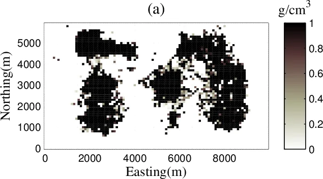
The methodology is then applied to real gravity data from the Mobrun ore body in northeastern Quebec, Canada. A 3‑D grid of 50 m cells is used, and the IRLS‑LSQR‑TUPRE workflow converges to a model that matches known drill‑hole information: high‑density zones are correctly located, and the model exhibits clear, compact bodies rather than diffuse anomalies. The reconstructed density distribution aligns with geological expectations and demonstrates the practical utility of the approach.

In summary, the paper makes three substantive contributions: (1) it integrates L₁‑norm regularization via IRLS to obtain sparse, geologically realistic gravity models; (2) it leverages LSQR to project large‑scale inversion problems onto a manageable subspace, drastically reducing computational demands; and (3) it introduces a truncated unbiased predictive risk estimator (TUPRE) for selecting the regularization parameter in the projected space, thereby avoiding the pitfalls of over‑regularization caused by the noisy tail of the spectrum. The combined framework delivers efficient, high‑resolution 3‑D gravity inversions and is readily extensible to other geophysical inverse problems such as magnetics, electromagnetic, or seismic tomography.