Fixed-Support Wasserstein Barycenters: Computational Hardness and Fast Algorithm

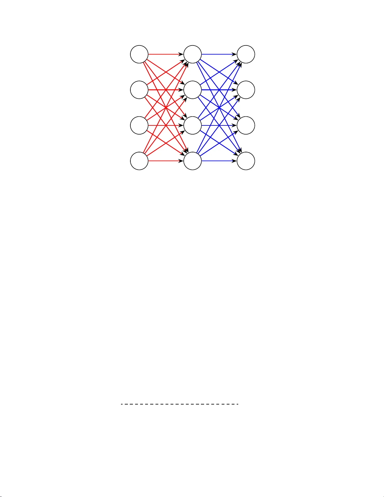
Fixed-Supp ort W asserste in Barycen ters: Computation al Hardness and F ast Algor ithm Tian yi Lin ⋄ Nhat Ho ⋆ Xi Chen ‡ Marco Cuturi ⊳,⊲ Mic hael I. Jordan ⋄ , † Departmen t of Electric al Engineering a n d Computer Sciences ⋄ Departmen t of S tatistics † Univ ersity of California, UC Berk eley Departmen t of S tatistics and Data S ciences, Unive r sit y of T exas, Austin ⋆ Stern S c ho ol of Business, New Y ork Universit y ‡ CREST - ENSAE ⊳ , Go ogle Brain ⊲ June 7, 2022 Abstract W e study the ﬁxed-supp ort W a sserstein barycenter problem (FS-WBP), whic h co nsists in co mputing the W ass erstein bar ycenter of m discrete probability measur es supp orted on a ﬁnite metric space of size n . W e show ﬁrst that the constraint matr ix arising from the standard linear programming (LP) r e pr esentation of the FS-WBP is not total ly unimo dular when m ≥ 3 and n ≥ 3 . This res ult reso lves an op en questio n p ertaining to the rela tionship betw e en the FS-WBP and the minimum-cost ﬂow (MCF) pro blem since it proves that the FS-WBP in the standard LP form is not an MCF pro blem when m ≥ 3 and n ≥ 3. W e also develop a pr ov ably fast de t erministic v aria nt of the celebrated iter ative Br e g man pro jection (IBP) algo rithm, named F astIBP , with a complexity b ound of e O ( mn 7 / 3 ε − 4 / 3 ), where ε ∈ (0 , 1) is the desired tole r ance. This complexity b ound is better than the best known complexity b ound of e O ( mn 2 ε − 2 ) for the IBP algor ithm in terms of ε , and that o f e O ( mn 5 / 2 ε − 1 ) fr o m accelera ted alternating minimizatio n algo rithm or acceler ated pr imal- dual adaptive gra dient alg orithm in ter ms of n . Finally , we c o nduct ex tens ive exp eriments with b oth synthet ic data and real images a nd demonstra te the fav o r able p er formance of the F astIBP alg orithm in practice . 1 In tro d uction Ov er the past decade, the W asserstein barycen ter p roblem [ Agueh and C arlier , 2011 ] (WBP) has serv ed as a found ation for theoretical analysis in a wide range of ﬁ elds, includ ing eco- nomics [ Carlier and Ek eland , 2010 , Chiapp ori et al. , 2010 ] and physics [ Buttazzo et al. , 2012 , Cotar et al. , 2013 , T r ou v´ e and Y ounes , 2005 ] to statistics [ Munc h et al. , 2015 , Ho et al. , 2017 , Sriv asta v a et al. , 2018 ], image and s h ap e analysis [ Rabin et al. , 2011 , Bonneel et al. , 2015 , 2016 ] and m achine learning [ Cuturi and Doucet , 2014 ]. Th e WBP pr oblem is related to the optimal transp ort (OT) prob lem, in that b oth are b ased on the W asserstein d istance, bu t the WBP is signiﬁcantl y harder. I t requir es the min imization of the su m of W asserstein distances, and t ypically considers m > 2 p robabilit y measures. I ts closest relativ e is th e m ultimarginal optimal transp ort problem [ Gangb o and Swiech , 1998 ], whic h also compares m m easures; see Villani [ 2008 ] for a compreh ensiv e treatmen t of OT th eory and Peyr ´ e and Cuturi [ 2019 ] for an in tr o duction of OT applications and algorithms. An ongoing fo cus of w ork in b ot h the WBP and the OT prob lem is the design of fast algo- rithms f or computing the relev an t distances and optima and the delineation of lo w er b ounds 1 that capture the computational hardness of these problems [ P eyr´ e and Cu turi , 2019 ]. F or the OT problem, Cuturi [ 2013 ] int r o duced the Sin khorn algorithm whic h has tr iggered signiﬁcan t progress [ Cuturi and P eyr´ e , 2016 , Genev a y et al. , 2016 , Altsch uler et al. , 2017 , Dvurec h en sky et al. , 2018 , Blanc het et al. , 2018 , Lin et al. , 2019b , Lahn et al. , 2019 , Quanru d , 2019 , Jambulapati et al. , 2019 , Lin et al. , 2019c ]. V ariants of the Sinkhorn and Greenkhorn algorithms [ Altsch uler et al. , 2017 , Dvu r ec hensky et al. , 2018 , Lin et al. , 2019b ] contin ue to serve as th e baseline approac h es in practice. As for the theoretical complexit y , the b est b ound is e O ( n 2 ε − 1 ) [ Blanc het et al. , 2018 , Quanr ud , 2019 , L ahn et al. , 2019 , J am bulapati et al. , 2019 ]. Moreo ver, Lin et al. [ 2019a ] pro vid ed a complexity b ound for the multimarginal OT p roblem. There has b een signiﬁ can t eﬀort devote d to the d ev elopmen t of fast algorithms in the case of m > 2 discr ete probabilit y m easur es [ Rabin et al. , 2011 , Cu turi and Doucet , 2014 , Carlier et al. , 2015 , Bonneel et al. , 2015 , Benamou et al. , 2015 , An d eres et al. , 2016 , Staib et al. , 2017 , Y e et al. , 2017 , Borgw ardt and Patt er s on , 2020 , Puccetti et al. , 2020 , Claici et al. , 2018 , Urib e et al. , 2018 , Dvurechenskii et al. , 2018 , Y ang et al. , 2018 , Le et al. , 2019 , Kroshn in et al. , 2019 , Gumino v et al. , 2019 , Ge et al. , 2019 , Borgw ardt and P atterson , 2019 ]. This work h as pro vid ed the foundation for p rogress on the WBP . An imp ortant step forwa r d was the prop osal of Cutu r i and Doucet [ 2014 ] to smo oth th e WBP using an entropic regularization, leading to a simple gradien t-descen t sc heme that was later imp ro ve d and generalized u nder the n ame of the iterativ e Bregman pr o ject ion (IBP) algorithm [ Benamou et al. , 2015 , Kroshnin et al. , 2019 ]. F urther pr ogress includes the semi-dual gradient d escen t [ Cuturi and P eyr´ e , 2016 , 2018 ], accel- erated primal-dual gradien t d escen t (APDA GD) [ Dvurec hensk ii et al. , 2018 , Kroshn in et al. , 2019 ], accele r ated IBP [ Guminov et al. , 2019 ], sto chastic gradient d escen t [ Claici et al. , 2018 ], distributed and parallel gradient descent [ Staib et al. , 2017 , Urib e et al. , 2018 ], alternating d i- rection metho d of m u ltipliers (ADMM) [ Y e et al. , 2017 , Y ang et al. , 201 8 ] and interior-p oint algorithm [ Ge et al. , 2019 ]. V ery recen tly , Kr oshnin et al. [ 2019 ] and Guminov et al. [ 2019 ] ha ve prop osed a no vel pr imal-dual framework that made it p ossible to derive complexit y b ound s for v arious algorithms, in clud ing IBP , accelerate d IBP and APD AGD . Concerning the computational hard ness of the WBP with free sup p ort, Anderes et al. [ 2016 ] p ro ved that the barycenter of m empirical measures is also an empirical measure with supp ort wh ose cardin alit y is at most the size of the union of the s u pp ort of the m measures, min u s m − 1. When m = 2 and the measures are b ound and the sup p ort is ﬁ xed, the computation of th e barycente r amoun ts to solving a net work ﬂo w pr oblem on a dir ected graph. Borgwa r d t and Pa tterson [ 2019 ] pro ved that ﬁnding a barycent er of s parse sup p ort is NP hard ev en in the simp le setting w hen m = 3. Ho wev er, their an alysis cannot b e extended to the ﬁxed-sup p ort WBP , where the sup p orts of the constituent m probabilit y measures are presp ec iﬁ ed . Con tribut ion. In this pap er, we r evisit the ﬁxed -supp ort W asserstein barycenter problem (FS-WBP) b etw een m discrete probabilit y measures supp orted on a presp eci ﬁ ed set of n p oint s . Our con tributions can b e su mmarized as f ollo w s: 1. W e prov e that the FS -WBP in the standard LP form is n ot a minimum-cost ﬂ o w (MCF) problem in general. In particular, w e show that the constrain t matrix arising f rom the standard LP representati on of the FS-WBP is totally unimo d ular when m ≥ 3 and n = 2 but not totally u nimo du lar wh en m ≥ 3 and n ≥ 3. Ou r results shed ligh t on the ne c essity of pr oblem r eformulation —e.g., en tropic regularization [ Cuturi and Doucet , 2014 , Benamou et al. , 2015 ] and blo c k reduction [ Ge et al. , 2019 ]. 2. W e prop ose a fast deterministic v arian t of the iterativ e Bregman pr o jecti on (IBP) al- 2 gorithm, named F astIBP , and pro vide a theoretical guarant ee for the algorithm. Let- ting ε ∈ (0 , 1) denote the target tolerance, the complexit y b ound of th e algorithm is e O ( mn 7 / 3 ε − 4 / 3 ), w hic h impro ves the complexity b oun d of e O ( mn 2 ε − 2 ) of the IBP algo- rithm [ Benamou et al. , 2015 ] in terms of ε and the complexit y b ound of e O ( mn 5 / 2 ε − 1 ) from the accelerated IBP and APD AG D algorithms in terms of n [ Kroshnin et al. , 2019 , Gumino v et al. , 2019 ]. W e cond u ct exp eriments on synthetic and real datasets and demonstrate that the F astIBP algorithm ac hieves the fav orable p erformance in pr ac- tice. Organization. The r emainder of the p ap er is organized as follo ws. In Section 2 , we pro vid e the basic setup for the entropic-regulariz ed FS-WBP and th e dual problem. In S ection 3 , w e present our compu tational hard ness r esu lts for the FS-WBP in the standard LP form . In Sections 4 , we p rop ose and analyze the F astIBP algorithm. W e present exp erim ental r esults on synthetic and real data in Section 5 and conclude in Section 6 . Notation. W e let [ n ] b e the set { 1 , 2 , . . . , n } and R n + b e the set of all vec tors in R n with nonnegativ e comp onents. 1 n and 0 n are the n -v ectors of ones and zeros. ∆ n stands for the probabilit y simplex: ∆ n = { u ∈ R n + : 1 ⊤ n u = 1 } . F or a smo oth fu nction f , we denote ∇ f and ∇ λ f as the fu ll gradien t and th e gradient with resp ect to a v ariable λ . F or x ∈ R n and 1 ≤ p ≤ ∞ , we write k x k p for its ℓ p -norm. F or X = ( X ij ) ∈ R n × n , the notations v ec ( X ) ∈ R n 2 and det( X ) stand f or the vect or r epresen tation and th e determinan t. The notations k X k ∞ = max 1 ≤ i,j ≤ n | X ij | and k X k 1 = P 1 ≤ i,j ≤ n | X ij | . T h e n otations r ( X ) = X 1 n and c ( X ) = X ⊤ 1 n . Let X , Y ∈ R n × n , the F rob enius an d Kron eck er inn er pro d uct are denoted b y h X, Y i and X ⊗ Y . Giv en the d imension n and ε , the notation a = O ( b ( n, ε )) stands for the u pp er b oun d a ≤ C · b ( n, ε ) wh ere C > 0 is indep end en t of n and ε , and a = e O ( b ( n, ε )) indicates the previous inequalit y where C dep ends only the logarithmic factors of n and ε . 2 Preliminaries and T ec hnical B ac k ground In th is section, w e in tro d uce the b asic setup of th e ﬁxed -su pp ort W assers tein barycen ter problem (FS-WBP), starting with the linear pr ogramming (LP) presenta tion and en tropic- regularized formulation and including a sp eciﬁcation of an appro ximate barycen ter. 2.1 Linear programming formula t ion F or p ≥ 1, let P p (Ω) b e the set of Borel probabilit y measures on Ω with ﬁn ite p -th moment . The W asserstein distance of order p ≥ 1 b etw een µ, ν ∈ P p (Ω) is deﬁn ed b y [ Villani , 2008 ]: W p ( µ, ν ) := inf π ∈ Π( µ,ν )  Z Ω × Ω d p ( x , y ) π ( d x , d y )  1 /p , (1) where d ( · , · ) is a metric on Ω and Π( µ, ν ) is the set of coup lings b et w een µ and ν . Giv en a w eight v ector ( ω 1 , ω 2 , . . . , ω m ) ∈ ∆ m for m ≥ 2, the Wasserstein b aryc enter [ Agueh and Carlier , 2011 ] of m probabilit y measures { µ k } m k =1 is a solution of the follo wing fu nctional min imization problem min µ ∈P p (Ω) m X k =1 ω k W p p ( µ, µ k ) . (2) 3 Because our goal is to pro v id e compu tational sc hemes to approxima tely solve the WBP , we need to pro vide a deﬁnition of an ε -appro ximate solution to the WBP . Deﬁnition 2.1. The pr ob ability me asur e b µ ∈ P p (Ω) is c al le d an ε -appro ximate barycenter if P m k =1 ω k W p p ( b µ, µ k ) ≤ P m k =1 ω k W p p ( µ ⋆ , µ k ) + ε wher e µ ⋆ is an optimal solution to pr oblem ( 2 ) . There are t wo main settings: (i) fr e e-supp ort Wasserstein b aryc enter , namely , w h en we optimize b oth the weig hts and supp orts of the barycen ter in Eq. ( 2 ); and (ii) ﬁxe d-supp ort Wasserstein b aryc enter , namely , wh en the supp orts of the b arycen ter are obtained f r om those from the p robabilit y measures { µ k } m k =1 and we optimize the we ights of the barycen ter in Eq. ( 2 ). The fr e e- supp ort WBP pr oblem is notoriously diﬃcult to solve. It can either b e solv ed using a solution to the multima r ginal-OT (MOT) pr oblem, as describ ed in detail by Agueh and Carlier [ 2011 ], or app ro ximated usin g alternativ e optimization tec hniqu es. Assumin g that eac h mea- sure is supp o r ted on n distinct p oint s, the WBP problem can b e solv ed exactly b y solving ﬁrst a MOT, to then compu te ( n − 1) m + 1 barycente r s of p oints in Ω (these b ary centers are exactly the supp ort of the barycentric measure). Solving a MOT is, ho wev er, equiv alen t to solving an LP with n m v ariables an d ( n − 1) m + 1 constrain ts. Th e other route, alternativ e optimization, r equires sp ecifying an initial guess for the barycente r , a discr ete measur e sup - p orted on k weigh ted p oin ts (where k is predeﬁn ed). O ne can then pro ceed b y up dating the lo cations of µ (or ev en add new on es) to decrease the ob jectiv e function in Eq. ( 2 ), b efore c hanging their weig hts. In the Euclidean setting with p = 2, the f ree-supp ort WBP is closely related to the clustering problem, and equ iv alen t to k -means wh en m = 1 [ Cuturi and Doucet , 2014 ]. Whereas solving the free-supp ort WBP using MOT r esults in a con vex (y et intrac table) problem, the alternating mimim ization approac h is not, in v ery muc h the same w ay that th e k -means p roblem is not, an d results in the minimization of a p iece-wise quadr atic function. On the other hand, the ﬁxe d- su pp ort WBP is c omp ar atively e asier to solve, and as such has playe d a r ole in r e al-world applic ations. F or in stance, in imaging sciences, pixels an d v o x els are supp orted on a p redeﬁned, ﬁnite grid. In these ap p lications, the barycente r and µ k measures share the same supp ort. In view of this, thr oughout the remainder of th e pap er, we let ( µ k ) m k =1 b e discrete probabil- it y measures and tak e the su pp ort p oints { x k i } i ∈ [ n ] to b e ﬁ x ed . Since { µ k } m k =1 ha ve the ﬁ xed supp ort, they are fully charac terized b y the w eights { u k } m k =1 . Accordingly , the supp ort of the barycen ter { b x i } i ∈ [ n ] is also ﬁxed and can b e p resp eciﬁed by { x k i } i ∈ [ n ] . Given this setup, the FS-WBP b etw een { µ k } m k =1 has the follo wing standard LP representa tion [ Cuturi and Doucet , 2014 , Benamou et al. , 2015 , Peyr ´ e and Cuturi , 2019 ]: min { X i } m i =1 ⊆ R n × n + m X k =1 ω k h C k , X k i , s.t. r ( X k ) = u k for all k ∈ [ m ] , c ( X k +1 ) = c ( X k ) for all k ∈ [ m − 1] , (3) where { X k } m k =1 and { C k } m k =1 ⊆ R n × ... × n + denote a set of tr ansp ortation plans and nonne gative c ost matric es and ( C k ) ij = d p ( x k i , b x j ) for all k ∈ [ m ]. The ﬁxed-sup p ort W asserstein barycen- ter u ∈ ∆ n is determined b y the weigh t P m k =1 ω k c ( X k ) and the su pp ort ( b x 1 , b x 2 , . . . , b x n ). F rom Eq. ( 3 ), the FS-WBP is an LP with 2 mn − n equ alit y constraints and mn 2 v ari- ables. This has inspired wo r k on solving the FS-WBP using classical optimization algo- rithms [ Ge et al. , 2019 , Y ang et al. , 2018 ]. Although p r ogress has b een made, the u nderstand- ing of the stru cture of FS-WBP via this app r oac h has remained limited. P articularly , while the OT problem [ Villani , 2008 ] is equiv alent to a minim um -cost ﬂo w (MCF) pr oblem, it re- mains unknown whether the FS-WBP is a MCF problem ev en in the simplest setting when m = 2. 4 2.2 En tropic regularized FS-WBP Using Cutu ri’s en tropic approac h to the OT pr oblem [ Cuturi , 2013 ], w e d eﬁne a regularized v ersion of the FS -WBP in Eq. ( 3 ), wh er e an en tropic regularization term is add ed to the W asserstein barycen ter ob jectiv e. The resulting formulat ion is as follo ws: min { X i } m i =1 ⊆ R n × n + m X k =1 ω k ( h C k , X k i − η H ( X k )) , s.t. r ( X k ) = u k for all k ∈ [ m ] , c ( X k +1 ) = c ( X k ) for all k ∈ [ m − 1] , (4) where η > 0 is the p arameter and H ( X ) := −h X , log ( X ) − 1 n 1 ⊤ n i denotes the en tropic regularization term. W e refer to Eq. ( 4 ) as entr opic r e gularize d FS-WBP . When η is large, the optimal v alue of entropic r egularized FS-WBP ma y yield a p oor app ro ximation of the cost of th e FS-WBP . T o guarantee a go o d app r o ximation, w e scale the parameter η as a function of th e desired accuracy . Deﬁnition 2.2. The pr ob ability ve c tor b u ∈ ∆ n is c al le d an ε -appr o ximate b arycen ter i f ther e exists a fe asible solution ( b X 1 , b X 2 , . . . , b X m ) ∈ R n × n + × · · · × R n × n + for the FS-WBP in Eq. ( 3 ) such that b u = P m k =1 ω k c ( b X k ) for al l k ∈ [ m ] and P m k =1 ω k h C k , b X k i ≤ P m k =1 ω k h C k , X ⋆ k i + ε wher e ( X ⋆ 1 , X ⋆ 2 , . . . , X ⋆ m ) is an optimal solution of the FS-WBP in Eq. ( 3 ) . With these d eﬁ nitions in min d, we develo p eﬃcien t algorithms for approxima tely solving the FS-WBP where the dep end ence on m , n and ε is comp etitiv e to state-of-the-art algo- rithms [ Kroshnin et al. , 2019 , Guminov et al. , 2019 ]. 2.3 Dual en t ropic regularized FS-WBP Using the dualit y theory of conv ex optimization [ Ro ck afellar , 1970 ], one dual form of en tropic regularized FS-WBP h as b een deriv ed b efore [ Cuturi and Doucet , 2014 , Kr osh nin et al. , 2019 ]. Diﬀering from the usu al 2-marginal or multimarginal OT [ Cuturi and P eyr´ e , 2018 , Lin et al. , 2019a ], the dual entropic regularized FS-WBP is a con ve x optimization problem with an aﬃne constrain t set. F orm ally , we ha ve min λ,τ ∈ R mn ϕ old ( λ, τ ) := m X k =1 ω k   X 1 ≤ i,j ≤ n e λ ki + τ kj − η − 1 ( C k ) ij − λ ⊤ k u k   , s.t. m X k =1 ω k τ k = 0 n . (5 ) Ho w ever, the ob jectiv e fu n ction in E q. ( 5 ) is not s uﬃcien tly smo oth b ecause of the su m of exp onents. This mak es the acceleration very c hallenging. In order to allevia te th is issue, w e turn to deriv e another smo oth dual form of en tropic-regularized FS-WBP . By introd ucing the d ual v ariables { α 1 , α 2 , . . . , α m , β 1 , β 2 , . . . , β m − 1 } ⊆ R n , w e deﬁn e the Lagrangian fu n ction of the entropic regularized FS-WBP in Eq. ( 4 ) as follo ws: L ( X 1 , . . . , X m , α 1 , . . . , α m , β 1 , . . . , β m − 1 ) (6) = m X k =1 ω k ( h C k , X k i − η H ( X k )) − m X k =1 α ⊤ k ( r ( X k ) − u k ) − m − 1 X k =1 β ⊤ k ( c ( X k +1 ) − c ( X k )) . By th e deﬁnition of H ( X ), the nonn egativ e constraint X ≥ 0 can b e n eglecte d . In order to deriv e the smo oth du al ob ject ive fu nction, we consid er the follo wing minimization problem: min { ( X 1 ,...,X m ): k X k k 1 =1 , ∀ k ∈ [ m ] } L ( X 1 , . . . , X m , α 1 , . . . , α m , β 1 , . . . , β m − 1 ) . 5 In the ab o ve problem, the ob jectiv e function is strongly con ve x. Thus, the op timal solution is unique. F or the simplicit y , we let α = ( α 1 , α 2 , . . . , α m ) ∈ R mn and β = ( β 1 , β 2 , . . . , β m − 1 ) ∈ R ( m − 1) n and assume the con ven tion β 0 = β m = 0 n . After the simple calculatio n s, the optimal solution ¯ X ( α, β ) = ( ¯ X 1 ( α, β ) , . . . , ¯ X m ( α, β )) has the follo wing form: ( ¯ X k ( α, β )) ij = e η − 1 ( ω − 1 k ( α ki + β k − 1 ,j − β kj ) − ( C k ) ij ) P 1 ≤ i,j ≤ n e η − 1 ( ω − 1 k ( α ki + β k − 1 ,j − β kj ) − ( C k ) ij ) for all k ∈ [ m ] , (7) Plugging Eq. ( 7 ) into Eq. ( 6 ) yields that the d ual form is: max α 1 ,...,α m ,β 1 ,...,β m − 1    − η m X k =1 ω k log   X 1 ≤ i,j ≤ n e η − 1 ( ω − 1 k ( α ki + β k − 1 ,j − β kj ) − ( C k ) ij )   + m X k =1 α ⊤ k u k    . In order to streamline our subsequent presen tation, we p erform a c hange of v ariables λ k = ( η ω k ) − 1 α k and τ k = ( η ω k ) − 1 ( β k − 1 − β k ) for all k ∈ [ m ]. Recall that β 0 = β m = 0 n , we hav e P m k =1 ω k τ k = 0 n . Putting these pieces together, we reformulat e the problem as min λ,τ ∈ R mn ϕ ( λ, τ ) := m X k =1 ω k log   X 1 ≤ i,j ≤ n e λ ki + τ kj − η − 1 ( C k ) ij   − m X k =1 ω k λ ⊤ k u k , s.t. m X k =1 ω k τ k = 0 n . T o fur ther sim p lify the ab o ve formulation, w e use the notation B k ( λ, τ ) ∈ R n × n b y ( B k ( λ k , τ k )) ij = e λ ki + τ kj − η − 1 ( C k ) ij ) for all ( i, j ) ∈ [ n ] × [ n ]. T o this end, we obtain the dual entr opic-r e gularize d FS-WBP pr oblem deﬁned by min λ,τ ∈ R mn ϕ ( λ, τ ) := m X k =1 ω k  log( k B k ( λ k , τ k ) k 1 ) − λ ⊤ k u k  , s.t. m X k =1 ω k τ k = 0 n . (8) Remark 2.1. The ﬁrst p art of the obje ctive function ϕ is in the form of the lo garithm of sum of exp onents while the se c ond p art is a line ar function. This is diﬀer ent fr om the obje ctive function u se d in pr evious dual entr opic r e gularize d O T pr oblem in Eq. ( 5 ) . We also note that Eq. ( 8 ) is a sp e cial instanc e of a softmax minimization pr oblem, and the obje ctive function ϕ is known to b e smo oth [ Nester ov , 2005 ] . Final ly, we p oint out that the same pr oblem was derive d in the c oncurr ent work by Guminov et al. [ 2019 ] and use d for analyzing the ac c eler ate d alternating minimization algorithm. In the r emainder of the p ap er, we also denote ( λ ⋆ , τ ⋆ ) ∈ R mn × R mn as an optimal solution of th e dual entropic regularized FS-WBP pr oblem in Eq. ( 8 ). 2.4 Prop erties of dual en tropic regularized FS-WBP In this section, we pr esen t seve r al useful prop erties of the du al entropic regularized MOT in Eq. ( 8 ). In particular, w e sh ow that there exists an optimal s olution ( λ ⋆ , τ ⋆ ) such that it h as an up p er b ound in terms of the ℓ ∞ -norm. Lemma 2.2. F or the dual entr opic r e gularize d FS-WBP, let ¯ C = max 1 ≤ k ≤ m k C k k ∞ and ¯ u = min 1 ≤ k ≤ m, 1 ≤ j ≤ n u k j , ther e exists an optimal solution ( λ ⋆ , τ ⋆ ) such that the fol low i ng ℓ ∞ -norm b ound holds true: k λ ⋆ k k ∞ ≤ R λ , k τ ⋆ k k ∞ ≤ R τ , for all k ∈ [ m ] , wher e R λ = 9 η − 1 ¯ C + 2 log ( n ) − log ( ¯ u ) and R τ = 4 η − 1 ¯ C . 6 Pr o of. First, we s ho w that there exists m pairs of optimal solutions { ( λ j , τ j ) } j ∈ [ m ] suc h that eac h of ( λ j , τ j ) satisﬁes that max 1 ≤ i ≤ n ( τ j k ) i ≥ 0 ≥ m in 1 ≤ i ≤ n ( τ j k ) i , for all k 6 = j. (9) Fixing j ∈ [ m ], we let ( b λ, b τ ) b e an optimal solution of the d ual en tropic regularized FS-WBP in Eq . ( 8 ). If b τ satisﬁes Eq. ( 9 ), the claim holds true for the ﬁxed j ∈ [ m ]. Otherwise, we deﬁne m − 1 shift terms give n by ∆ b τ k = max 1 ≤ i ≤ n ( b τ k ) i + min 1 ≤ i ≤ n ( b τ k ) i 2 ∈ R for all k 6 = j, and let ( λ j , τ j ) w ith τ j k = b τ k − ∆ b τ k 1 n , λ j k = b λ k + ∆ b τ k 1 n , for all k 6 = j, τ j j = b τ j + ( P k 6 = j ( ω k ω j )∆ b τ k ) 1 n , λ j j = b λ j − ( P k 6 = j ( ω k ω j )∆ b τ k ) 1 n . Using this constru ction, we h a v e ( λ j k ) i + ( τ j k ) i ′ = ( b λ k ) i + ( b τ k ) i ′ for all i, i ′ ∈ [ n ] and all k ∈ [ m ]. This implies that B k ( b λ k , b τ k ) = B k ( λ k ′ k , τ k ′ k ) for all k ∈ [ m ]. F urthermore, w e ha v e m X k =1 ω k τ j k = m X k =1 ω k b τ k , m X k =1 ω k ( λ j k ) ⊤ u k = m X k =1 ω k b λ ⊤ k u k . Putting these pieces together yields ϕ ( λ j , τ j ) = ϕ ( b λ, b τ ). Moreo v er, by the deﬁnition of ( λ j , τ j ) and m − 1 shift terms, τ j satisﬁes E q . ( 9 ). Th erefore, we conclude that ( λ j , τ j ) is an optimal solution that satisﬁes Eq. ( 9 ) for the ﬁxed j ∈ [ m ]. Since j ∈ [ m ] is chosen arbitarily , we can ﬁnd the d esired pairs of optimal solutions { ( λ j , τ j ) } j ∈ [ m ] satisfying Eq. ( 9 ) by r ep eating the ab o ve argument m times. F urthermore, eac h of ( λ j , τ j ) must satisfy the optimalit y condition for Eq. ( 8 ) for all k ∈ [ m ]. Fixing j ∈ [ m ], there exists z ∈ R n suc h that m X k =1 ω k τ j k = 0 n and B k ( λ j k , τ j k ) ⊤ 1 n k B k ( λ j k , τ j k ) k 1 − z = 0 n for all k ∈ [ m ] . (10) By the deﬁnition of B k ( · , · ), we h a v e τ j k = log( z ) + log( k B k ( λ j k , τ j k ) k 1 ) 1 n − log ( e − η − 1 C k diag( e λ j k ) 1 n ) for all k ∈ [ m ] . This together with the ﬁrst equalit y in Eq. ( 10 ) yields that τ j k = m X l =1 ω l log( e − η − 1 C l diag( e λ j l ) 1 n ) − log( e − η − 1 C k diag( e λ j k ) 1 n ) for all k ∈ [ m ] . F or eac h i ∈ [ n ] and l ∈ [ m ], by the nonn egativit y of eac h en try of C l , we h a ve − η − 1 k C l k ∞ + log( 1 ⊤ n e λ j l ) ≤ [log( e − η − 1 C l diag( e λ j l ) 1 n )] i ≤ log ( 1 ⊤ n e λ j l ) . Putting these pieces toget h er yields max 1 ≤ i ≤ n ( τ j k ) i − min 1 ≤ i ≤ n ( τ j k ) i ≤ η − 1 k C k k ∞ + m X l =1 ω l η − 1 k C l k ∞ for all k ∈ [ m ] . (11) 7 Com bin ing Eq. ( 9 ) and Eq. ( 11 ) yields th at k τ j k k ∞ ≤ η − 1 k C k k ∞ + m X l =1 ω l η − 1 k C l k ∞ for all k 6 = j. (12) Since P m k =1 ω k τ j k = 0 n , we h a ve k τ j j k ∞ ≤ ω − 1 j X k 6 = j ω k k τ j k k ∞ ≤ ( η ω j ) − 1 X k 6 = j ω k k C k k ∞ + ( η ω j ) − 1 (1 − ω j ) m X k =1 ω k k C k k ∞ . Finally , we pro ce ed to the k ey part and deﬁne the a verag ing iterate λ ⋆ = m X j =1 ω j λ j , τ ⋆ = m X j =1 ω j τ j . Since ϕ is con ve x and ( ω 1 , ω 2 , . . . , ω m ) ∈ ∆ m , we ha ve ϕ ( λ ⋆ , τ ⋆ ) ≤ P m j =1 ω j ϕ ( λ j , τ j ) an d P m k =1 ω k τ ⋆ k = 0 n . S ince ( λ j , τ j ) are optimal solutions for all j ∈ [ m ], we conclud e that ( λ ⋆ , τ ⋆ ) is an optimal solution. Without loss of generalit y , we assu me that ( λ ⋆ , τ ⋆ ) satisﬁes that max 1 ≤ i ≤ n ( λ ⋆ k ) i ≥ 0 ≥ min 1 ≤ i ≤ n ( λ ⋆ k ) i , for all k ∈ [ m ] . (13) Indeed, if λ ⋆ do es n ot satisfy the ab ov e condition, w e deﬁne m shift terms giv en by ∆ λ ⋆ k = max 1 ≤ i ≤ n ( λ ⋆ k ) i + min 1 ≤ i ≤ n ( λ ⋆ k ) i 2 ∈ R for all k ∈ m, and let λ ⋆ k = λ ⋆ k − ∆ λ ⋆ k 1 n , for all k ∈ [ m ] . The ab ov e op erat ion will not c hange the v alue of ϕ ( λ ⋆ , τ ⋆ ) such th at ( λ ⋆ , τ ⋆ ) is a desired optimal solution whic h satisﬁes Eq. ( 13 ). The r emainin g step is to show that k λ ⋆ k k ∞ ≤ R λ and k τ ⋆ k k ∞ ≤ R τ for all k ∈ [ m ]. More sp eciﬁcally , w e ha ve k τ ⋆ k k ∞ ≤ m X j =1 ω j k τ j k k ∞ = ω k k τ k k k ∞ + X j 6 = k ω j k τ j k k ∞ ≤ η − 1 X l 6 = k ω l k C l k ∞ + η − 1 (1 − ω k ) m X l =1 ω l k C l k ∞ + η − 1 (1 − ω k )( k C k k ∞ + m X l =1 ω l k C l k ∞ ) ≤ η − 1 k C k k ∞ + 3 η − 1 m X l =1 ω l k C l k ∞ ≤ 4 η − 1 ¯ C = R τ . Since ( λ ⋆ , τ ⋆ ) is an optimal solution, it satisﬁes the optimalit y condition for Eq. ( 8 ). F ormally , w e ha ve B k ( λ ⋆ k , τ ⋆ k ) 1 n k B k ( λ ⋆ k , τ ⋆ k ) k 1 − u k = 0 n for all k ∈ [ m ] . (14) By the deﬁnition of B k ( · , · ), we h a v e λ ⋆ k = log ( u k ) + log( k B k ( λ ⋆ k , τ ⋆ k ) k 1 ) 1 n − log( e − η − 1 C k diag( e τ ⋆ k ) 1 n ) for all k ∈ [ m ] . 8 This implies that max 1 ≤ i ≤ n ( λ ⋆ k ) i ≤ η − 1 k C k k ∞ + log ( n ) + k τ ⋆ k k ∞ + log ( k B k ( λ ⋆ k , τ ⋆ k ) k 1 ) , min 1 ≤ i ≤ n ( λ ⋆ k ) i ≥ log( ¯ u ) − log ( n ) − k τ ⋆ k k ∞ + log ( k B k ( λ ⋆ k , τ ⋆ k ) k 1 ) . Therefore, we ha ve max 1 ≤ i ≤ n ( λ ⋆ k ) i − min 1 ≤ i ≤ n ( λ ⋆ k ) i ≤ η − 1 k C k k ∞ + 2 log ( n ) − log ( ¯ u ) + 2 k τ ⋆ k k ∞ . T ogether w ith Eq. ( 13 ), we conclude that k λ ⋆ k k ∞ ≤ η − 1 k C k k ∞ + 2 log ( n ) − log( ¯ u ) + 2 k τ ⋆ k k ∞ . This completes the p ro of.  Remark 2.3. L emma 2.2 is analo gous to [ Lin et al. , 2019b , L emma 3.2] for the OT pr oblem. However, the dual entr opic-r e gularize d FS-WBP is mor e c omplex and r e quir es a novel c onstruc- tive i ter ate, ( λ ⋆ , τ ⋆ ) = P m j =1 ω j ( λ j , τ j ) . Mor e over, the te chniques in Kr oshnin et al. [ 2019 ] ar e not applic able for the analysis of the F astI BP algorithm, and, ac c or dingly, L emma 2.2 is cru- cial for the analysis. The upp er b ound for the ℓ ∞ -norm of the optimal solution of dual en tropic-regularized FS-WBP in Lemma 2.2 leads to the follo wing straigh tforward consequence. Corollary 2.4. F or the dual entr opic r e gu larize d FS-WBP, ther e exists an optimal solution ( λ ⋆ , τ ⋆ ) such that for al l k ∈ [ m ] , k λ ⋆ k k ≤ √ nR λ , k τ ⋆ k k ≤ √ nR τ , for all k ∈ [ m ] , wher e R λ , R τ > 0 ar e deﬁne d in L emma 2.2 . Finally , w e observe that ϕ can b e decomp osed into the w eighte d sum of m functions and pro ve that eac h comp onent fun ction ϕ k has Lipsc h itz con tinuous gradien t with the constant 4 in the follo wing lemma. Lemma 2.5. The fol lowing statement holds true, ϕ ( λ, τ ) = P m k =1 ϕ k ( λ k , τ k ) wher e ϕ k ( λ k , τ k ) = log( 1 ⊤ n B k ( λ k , τ k ) 1 n ) − λ ⊤ k u k for al l k ∈ [ m ] . Mor e over, e ach ϕ k has Li pschitz c ontinuous gr a- dient in ℓ 2 -norm and the Lipschitz c onstant is upp er b ounde d by 4 . F ormal ly, k∇ ϕ k ( λ, τ ) − ∇ ϕ k ( λ ′ , τ ′ ) k ≤ 4      λ τ  −  λ ′ τ ′      for all k ∈ [ m ] . which is e quivalent to ϕ ( λ ′ , τ ′ ) − ϕ ( λ, τ ) ≤  λ ′ − λ τ ′ − τ  ⊤ ∇ ϕ ( λ, τ ) + 2 m X k =1 ω k      λ ′ k − λ k τ ′ k − τ k      2 ! . Pr o of. Th e ﬁ rst statemen t directly follo ws from the deﬁn ition of ϕ in Eq. ( 8 ). F or the second statemen t, we pr o vide the explicit form of the gradient of ϕ k as follo w s, ∇ ϕ k ( λ, τ ) =   B k ( λ,τ ) 1 n 1 ⊤ n B k ( λ,τ ) 1 n − u k B k ( λ,τ ) ⊤ 1 n 1 ⊤ n B k ( λ,τ ) 1 n   . 9 No w w e construct the follo wing ent r opic r egularized OT p roblem, min X : k X k 1 =1 h C k , X i − η H ( X ) , s.t. X 1 n = (1 /n ) 1 n , X ⊤ 1 n = (1 /n ) 1 n . Since the fun ction − H ( X ) is strongly con vex with r esp ect to the ℓ 1 -norm on the probability simplex Q ⊆ R n 2 , the ab o ve en trop ic regularized OT p roblem is a sp eci al case of the follo win g linearly constrained con vex optimization problem: min x ∈ Q f ( x ) , s.t. Ax = b, where f is str on gly con v ex with resp ect to the ℓ 1 -norm on the set Q . W e use the ℓ 2 -norm for the dual space of the L agrange m ultipliers. By Nestero v [ 2005 , Th eorem 1] and the fact that k A k 1 → 2 = 2, the dual ob jectiv e f unction ˜ ϕ k satisﬁes th e follo wing inequalit y: k∇ ˜ ϕ k ( α, β ) − ∇ ˜ ϕ k ( α ′ , β ′ ) k ≤ 4 η      α β  −  α ′ β ′      . Recall that the function ˜ ϕ k is given by ˜ ϕ k ( α, β ) = η log   n X i,j =1 e − ( C k ) ij − α i − β j η − 1   − h α, u i − h β , v i + η . This together with the deﬁnition of B k ( · , · ) implies that ∇ ˜ ϕ k ( α, β ) =    B k ( η − 1 α − (1 / 2) 1 n ,η − 1 β − (1 / 2) 1 n ) 1 n 1 ⊤ n B k ( η − 1 α − (1 / 2) 1 n ,η − 1 β − (1 / 2) 1 n ) 1 n − u B k ( η − 1 α − (1 / 2) 1 n ,η − 1 β − (1 / 2) 1 n ) ⊤ 1 n 1 ⊤ n B k ( η − 1 α − (1 / 2) 1 n ,η − 1 β − (1 / 2) 1 n ) 1 n − v    P erformin g the change of v ariable λ = η − 1 α − (1 / 2) 1 n and τ = η − 1 β − (1 / 2) 1 n (resp. λ ′ and τ ′ ), we ha ve k∇ ϕ k ( λ, τ ) − ∇ ϕ k ( λ ′ , τ ′ ) k = k∇ ˜ ϕ k ( η ( λ + (1 / 2) 1 n ) , η ( τ + (1 / 2) 1 n )) − ∇ ˜ ϕ k ( η ( λ ′ + (1 / 2) 1 n ) , η ( τ ′ + (1 / 2) 1 n )) k ≤ 4      λ ′ − λ τ ′ − τ      . This completes the p ro of.  Remark 2.6. It is worthy noting that L emma 2.5 exploits the de c omp osable structur e of the dual function ϕ , and give s the a weighte d smo othness i ne quality. This ine q uality is ne c essary for deriving the c omplexity b ound which dep ends line arly on the numb er of pr ob ability me asur es. 3 Computational Hardness In this section, w e analyze the compu tational hardn ess of the FS-WBP in Eq. ( 3 ). After in tro d ucing some c haracterization theorems in com binatorial optimization, w e sho w that the FS-WBP in E q . ( 3 ) is a minim um-cost ﬂo w (MCF) p roblem wh en m = 2 and n ≥ 3 but not when m ≥ 3 and n ≥ 3. 10 3.1 Com binatorial t ec hniques W e present some classical resu lts in com binatorial optimization and graph theory , including Ghouila-Houri’s celebrated c h aracterization theorem [ Ghouila-Houri , 1962 ]. Deﬁnition 3.1. A total ly unimo dular (TU) matrix is one for which every squar e submatrix has determinant − 1 , 0 or 1 . Prop osition 3.1 (Ghouila-Houri) . A {− 1 , 0 , 1 } -value d matrix A ∈ R m × n is TU if and only if for e ach I ⊆ [ m ] ther e is a p artition I = I 1 ∪ I 2 so that P i ∈ I 1 a ij − P i ∈ I 2 a ij ∈ {− 1 , 0 , 1 } for j ∈ [ n ] . The second r esult [ Berge , 2001 , Th eorem 1, Chapter 15] sh o ws th at th e incidence matrices of d irected graphs and 2-colorable undir ected graphs are T U. Prop osition 3.2. L et A b e a {− 1 , 0 , 1 } -value d matrix. Then A is TU if e ach c olumn c ontains at most two nonzer o entries and al l r ows ar e p artitione d into two sets I 1 and I 2 such that: If two nonzer o entries of a c olumn have the same sign, they ar e in diﬀer ent sets. If these two entries have diﬀer ent signs, they ar e in the same set. Finally , we c h aracterize the constrain t matrix arising in a MCF problem. Deﬁnition 3.2. The MCF pr oblem ﬁnds the che ap est p ossible way of sending a c ertain amount of ﬂow thr ough a ﬂow network. F ormal ly, min P ( u,v ) ∈ E f ( u, v ) · a ( u, v ) s.t. f ( u, v ) ≥ 0 , f or all ( u, v ) ∈ E , f ( u, v ) ≤ c ( u, v ) for all ( u, v ) ∈ E , f ( u, v ) = − f ( v , u ) for all ( u, v ) ∈ E , P ( u,w ) ∈ E or ( w, u ) ∈ E f ( u, w ) = 0 , P w ∈ V f ( s, w ) = d and P w ∈ V f ( w, t ) = d. The ﬂow network G = ( V , E ) is a dir e c te d gr aph G = ( V , E ) with a sour c e vertex s ∈ V and a sink v e rtex t ∈ V , wher e e ach e dge ( u, v ) ∈ E has c ap acity c ( u, v ) > 0 , ﬂow f ( u, v ) ≥ 0 and c ost a ( u, v ) , with most MCF algorithms supp orting e dges with ne gative c osts. The c ost of sending this ﬂow along an e dge ( u, v ) is f ( u, v ) · a ( u, v ) . The pr oblem r e quir es an amount of ﬂow d to b e sent f r om sour c e s to sink t . Th e deﬁnition of the pr oblem is to minimize the total c ost of the ﬂow over al l e dges. Prop osition 3.3. The c onstr aint matrix arising in a MCF pr oblem is TU and its r ows ar e c ate gorize d into a single set using P r op osition 3.2 . Pr o of. The stand ard LP r epresen tation of the MCF p roblem is min x ∈ R | E | c ⊤ x, s.t. Ax = b, l ≤ x ≤ u. where x ∈ R | E | with x j b eing th e ﬂo w through arc j , b ∈ R | V | with b i b eing external supply at no de i and 1 ⊤ b = 0, c j is unit cost of ﬂo w through arc j , l j and u j are low er and upp er b ound s on ﬂo w through arc j and A ∈ R | V |×| E | is the arc-no de incidence matrix with ent r ies A ij =    − 1 if arc j starts at no d e i 1 if arc j ends at no d e i 0 otherwise . 11 u 11 u 12 u 13 u 14 0 0 0 0 u 21 u 22 u 23 u 24 Figure 1: Represent the FS-WBP in Eq. ( 3 ) as a MCF pr oblem when ( m, n ) = (2 , 4). Since eac h arc has tw o endp oin ts, the constrain t matrix A is a {− 1 , 0 , 1 } -v alued matrix in whic h eac h column con tains t wo n onzero entries 1 and − 1. Using Pr op osition 3.2 , we obtain that A is TU and the ro ws of A are categorized int o a single set.  3.2 Main result W e present ou r main results on the computational hard ness of th e FS-WBP in Eq. ( 3 ). First, the FS-WBP in this LP form is an MCF pr ob lem wh en m = 2 and n ≥ 2; see Figure 1 for the graph w hen ( m, n ) = (2 , 4). In d eed, it is a transp ortatio n problem w ith n warehouses, n transs hipment centers and n r etail outlets. Eac h u 1 i is the amount of sup p ly pro vid ed by the i th warehouse and eac h u 2 j is the amount of demand requested by the j th r etail outlet. ( X 1 ) ij is the ﬂow sent from i th w arehouse to the j th transshipment cen ter and ( X 2 ) ij is the ﬂo w sent from th e i th tr an s shipment center to the j th retail outlet. ( C 1 ) ij and ( C 2 ) ij refer to the u nit cost of the corresp onding ﬂow. See [ Anderes et al. , 2016 , P age 400]. Pro ceed to the setting m ≥ 3, it is un clear whether the graph r epresen tation of the FS- WBP carries ov er. Instead, w e turn to algebraic tec h n iques and p ro vide an explicit form as follo ws: min m X k =1 h C k , X k i , s.t.                      − E · · · · · · · · · · · · . . . E . . . . . . . . . . . . . . . . . . . . . . . . . . . . . . . . . ( − 1) m − 1 E . . . . . . . . . . . . . . . ( − 1) m E G − G . . . . . . . . . . . . − G G . . . . . . . . . . . . . . . . . . . . . · · · · · · · · · ( − 1) m G ( − 1) m +1 G                                    vec ( X 1 ) vec ( X 2 ) . . . . . . . . . . . . vec ( X m )               =               − u 1 u 2 . . . ( − 1) m − 1 u m − 1 ( − 1) m u m 0 n . . . 0 n               , (15) 12 where E = I n ⊗ 1 ⊤ n ∈ R n × n 2 and G = 1 ⊤ n ⊗ I n ∈ R n × n 2 . Eac h column of the constrain t matrix arising in Eq. ( 15 ) has either 2 or 3 nonzero en tr ies in {− 1 , 0 , 1 } . I n the follo win g theorem, w e study the structure of the constrain t matrix wh en m ≥ 3 and n = 2. Theorem 3.4. The c onstr aint matrix arising in Eq. ( 15 ) is TU when m ≥ 3 and n = 2 . Pr o of. When n = 2, the constrain t matrix A has E = I 2 ⊗ 1 ⊤ 2 and G = 1 ⊤ 2 ⊗ I 2 . The matrix A ∈ R (4 m − 2) × 4 m is a {− 1 , 0 , 1 } -v alued matrix with several r edundant ro w s and eac h column has at most thr ee nonzero en tries in {− 1 , 0 , 1 } . No w we simplify the matrix A by r emoving a sp eciﬁc set of redundant ro w s . In p articular, we observe th at X i ∈{ 1 , 2 , 3 , 4 , 2 m +1 , 2 m +2 } a ij = 0 , ∀ j ∈ [4 m ] , whic h implies that th e (2 m + 2)th r ow is r edundant. Similarly , w e ha ve X i ∈{ 3 , 4 , 5 , 6 , 2 m +3 , 2 m +4 } a ij = 0 , ∀ j ∈ [4 m ] , whic h implies that the (2 m + 3)th ro w is redun dant . Using this argumen t, we remov e m − 1 ro ws from the last 2 m − 2 ro w s. T h e resu lting matrix ¯ A ∈ R (3 m − 1) × 4 m has very n ice structure suc h th at eac h column has only tw o nonzero entries 1 and − 1; see the follo wing matrix when m is o dd: ¯ A =                     − E · · · · · · · · · · · · . . . E . . . . . . . . . . . . . . . . . . . . . . . . . . . . . . . . . ( − 1) m − 1 E . . . . . . . . . . . . . . . ( − 1) m E 1 ⊤ 2 ⊗ e 1 − 1 ⊤ 2 ⊗ e 1 . . . . . . . . . . . . − 1 ⊤ 2 ⊗ e 2 1 ⊤ 2 ⊗ e 2 . . . . . . . . . . . . . . . . . . . . . · · · · · · · · · ( − 1) m 1 ⊤ 2 ⊗ e 2 ( − 1) m +1 1 ⊤ 2 ⊗ e 2                     . where e 1 and e 2 are r esp ectiv ely the ﬁ r st and second standard basis (ro w) vect ors in R 2 . F ur- thermore, the rows of ¯ A are categorized in to a sin gle set so that the criterion in Prop osition 3.2 holds tru e (the d ashed line in th e formulation of ¯ A s er ves as a partition of this single set int o t wo sets). Using Prop osition 3.2 , we conclude that ¯ A is T U.  T o facilitate the r eader, w e provide an illustrativ e counte r example for showing that the FS-WBP in Eq. ( 15 ) is n ot an MCF pr oblem when m = 3 and n = 3. Example 3.1. When m = 3 and n = 3 , the c onstr aint matrix is A =       − I 3 ⊗ 1 ⊤ 3 0 3 × 9 0 3 × 9 0 3 × 9 I 3 ⊗ 1 ⊤ 3 0 3 × 9 0 3 × 9 0 3 × 9 − I 3 ⊗ 1 ⊤ 3 1 ⊤ 3 ⊗ I 3 − 1 ⊤ 3 ⊗ I 3 0 3 × 9 0 3 × 9 − 1 ⊤ 3 ⊗ I 3 1 ⊤ 3 ⊗ I 3       . 13 Setting the set I = { 1 , 4 , 7 , 10 , 11 , 13 , 15 } and letting e 1 , e 2 and e 3 b e the ﬁrst, se c ond and thir d standa r d b asis r ow v e ctors in R n , the r e su lting matrix with the r ows in I i s R =           − e 1 ⊗ 1 ⊤ 3 0 1 × 9 0 1 × 9 0 1 × 9 e 1 ⊗ 1 ⊤ 3 0 1 × 9 0 1 × 9 0 1 × 9 − e 1 ⊗ 1 ⊤ 3 1 ⊤ 3 ⊗ e 1 − 1 ⊤ 3 ⊗ e 1 0 1 × 9 1 ⊤ 3 ⊗ e 2 − 1 ⊤ 3 ⊗ e 2 0 1 × 9 0 1 × 9 − 1 ⊤ 3 ⊗ e 1 1 ⊤ 3 ⊗ e 1 0 1 × 9 − 1 ⊤ 3 ⊗ e 3 1 ⊤ 3 ⊗ e 3           . Inste ad of c onsidering al l c olumns of R , it suﬃc e s to show that no p artition of I guar ante es for any j ∈ { 1 , 2 , 11 , 12 , 13 , 19 , 21 } that X i ∈ I 1 R ij − X i ∈ I 2 R ij ∈ {− 1 , 0 , 1 } . We write the submatrix of R with these c olumns as ¯ R =           − 1 − 1 0 0 0 0 0 0 0 1 1 0 0 0 0 0 0 0 0 − 1 − 1 1 0 0 0 − 1 0 0 0 1 − 1 0 0 0 0 0 0 0 0 − 1 1 0 0 0 0 − 1 0 0 1           First, we claim that r ows 1 , 2 , 4 , 5 and 7 ar e in the same set I 1 . Inde e d, c olumns 1 and 2 imply that r ows 1 , 4 and 5 ar e in the same set. Column 3 and 4 imply that r ows 2 , 5 and 7 ar e in the same se t. Pu tting these pie c es to gether yields the desir e d claim. Then we c onsider the set that the r ow 6 b e longs to and claim a c ontr adiction. Inde e d, r ow 6 c an not b e in I 1 sinc e c olumn 5 implies that r ows 4 and 6 ar e not in the same set. However, r ow 6 must b e in I 1 sinc e c olumns 6 and 7 imply that r ows 3 , 6 and 7 ar e in the same set. Putting these pie c es to gether yie lds the desir e d c ontr adiction. Final ly, by using Pr op ositions 3.1 and 3.3 , we c onclude that A is not TU and pr oblem ( 15 ) is not a MCF pr oblem when m = 3 and n = 3 . Finally , we p r o ve that the FS -WBP in E q . ( 15 ) is not a MCF when m ≥ 3 and n ≥ 3. The b asic idea is to extend the constru ction in Example 3.1 to the general case. Theorem 3.5. The FS-WBP in Eq. ( 15 ) is not a MCF pr oblem when m ≥ 3 and n ≥ 3 . Pr o of. W e u se the p ro of by con tradiction. In particular, assum e that problem ( 15 ) is a MCF problem when m ≥ 3 and n ≥ 3, Prop osition 3.3 implies that the constrain t matrix A is TU. Sin ce A is a {− 1 , 0 , 1 } -v alued matrix, Prop ositi on 3.1 fu rther implies that for eac h set I ⊆ [2 mn − n ] there is a partition I 1 , I 2 of I su c h that X i ∈ I 1 a ij − X i ∈ I 2 a ij ∈ {− 1 , 0 , 1 } , ∀ j ∈ [ mn 2 ] . (16) In what follo ws, for an y giv en m ≥ 3 and n ≥ 3, we construct a set of ro ws I such that no partition of I guarantees that Eq. ( 16 ) holds tru e. F or the ease of presentati on, we rewrite 14 the m atrix A ∈ R (2 mn − n ) × mn 2 as follo ws, A =                     − I n ⊗ 1 ⊤ n · · · · · · · · · · · · . . . I n ⊗ 1 ⊤ n . . . . . . . . . . . . . . . . . . . . . . . . . . . . . . . . . ( − 1) m − 1 I n ⊗ 1 ⊤ n . . . . . . . . . . . . . . . ( − 1) m I n ⊗ 1 ⊤ n 1 ⊤ n ⊗ I n − 1 ⊤ n ⊗ I n . . . . . . . . . . . . − 1 ⊤ n ⊗ I n 1 ⊤ n ⊗ I n . . . . . . . . . . . . . . . . . . . . . · · · · · · · · · ( − 1) m 1 ⊤ n ⊗ I n ( − 1) m +1 1 ⊤ n ⊗ I n                     . Setting the set I = { 1 , n + 1 , 2 n + 1 , 3 n + 1 , 3 n + 2 , 4 n + 1 , 4 n + 3 } and letting e 1 , e 2 and e 3 b e th e ﬁ rst, second and third standard basis r o w vec tors in R n , th e r esulting matrix with the ro ws in I is R =           − e 1 ⊗ 1 ⊤ n 0 1 × n 2 0 1 × n 2 0 1 × n 2 · · · 0 1 × n 2 0 1 × n 2 e 1 ⊗ 1 ⊤ n 0 1 × n 2 0 1 × n 2 · · · 0 1 × n 2 0 1 × n 2 0 1 × n 2 − e 1 ⊗ 1 ⊤ n 0 1 × n 2 · · · 0 1 × n 2 1 ⊤ n ⊗ e 1 − 1 ⊤ n ⊗ e 1 0 1 × n 2 0 1 × n 2 · · · 0 1 × n 2 1 ⊤ n ⊗ e 2 − 1 ⊤ n ⊗ e 2 0 1 × n 2 0 1 × n 2 · · · 0 1 × n 2 0 1 × n 2 − 1 ⊤ n ⊗ e 1 1 ⊤ n ⊗ e 1 0 1 × n 2 · · · 0 1 × n 2 0 1 × n 2 − 1 ⊤ n ⊗ e 3 1 ⊤ n ⊗ e 3 0 1 × n 2 · · · 0 1 × n 2           . Instead of considering all columns of R , it suﬃces to s h o w that no partition of I guaran tees X i ∈ I 1 R ij − X i ∈ I 2 R ij ∈ {− 1 , 0 , 1 } , for all j ∈ { 1 , 2 , n 2 + 2 , n 2 + 3 , n 2 + n + 1 , 2 n 2 + 1 , 2 n 2 + 3 } . W e write the submatrix of R with these column s as ¯ R =           − 1 − 1 0 0 0 0 0 0 0 1 1 0 0 0 0 0 0 0 0 − 1 − 1 1 0 0 0 − 1 0 0 0 1 − 1 0 0 0 0 0 0 0 0 − 1 1 0 0 0 0 − 1 0 0 1           . Applying th e same argum en t used in Examp le 3.1 , we obtain from P r op ositions 3.1 and 3.3 that A is not TU w hen m ≥ 3 and n ≥ 3, whic h is a con tradiction. As a consequ en ce, the conclusion of the theorem follo ws.  Remark 3.6. The or em 3.5 r esolves an op en question and p artial ly explains why the dir e ct applic ation of network ﬂow algorithms to the FS-WBP in Eq . ( 15 ) is ineﬃci e nt. H owever, this do es not eliminate the p ossibility that the FS-WBP is e q u ivalent to some other LP with go o d c omplexity. F or example, Ge et al. [ 2019 ] have r e c e ntly suc c essfu l ly identiﬁe d an e quivalent 15 Algorithm 1: F as tIBP ( { C k , u k } k ∈ [ m ] , ε ) Initialization: t = 0, θ 0 = 1 a nd ˇ λ 0 = ˜ λ 0 = ˇ τ 0 = ˜ τ 0 = 0 mn . while E t > ε do Step 1: Compute  ¯ λ t ¯ τ t  = (1 − θ t )  ˇ λ t ˇ τ t  + θ t  ˜ λ t ˜ τ t  . Step 2: Compute r k = r ( B k ( ¯ λ t k , ¯ τ t k )) a nd c k = c ( B k ( ¯ λ t k , ¯ τ t k )) for all k ∈ [ m ] a nd per form ˜ λ t +1 k = ˜ λ t k − 1 4 θ t  r k 1 ⊤ n r k − u k  , for all k ∈ [ m ] , ˜ τ t +1 = argmin P m k =1 ω k τ k = 0 n m X k =1 ω k  ( τ k − ¯ τ t k ) ⊤ c k 1 ⊤ n c k + 2 θ t k τ k − ˜ τ t k k 2  . Step 3: Compute  b λ t b τ t  =  ¯ λ t ¯ τ t  + θ t  ˜ λ t +1 ˜ τ t +1  − θ t  ˜ λ t ˜ τ t  . Step 4: Compute  ´ λ t ´ τ t  = argmin  ϕ ( λ, τ ) |  λ τ  ∈  ˇ λ t ˇ τ t  ,  b λ t b τ t  . Step 5a: Compute c k = c ( B k ( ´ λ t k , ´ τ t k )) for all k ∈ [ m ]. Step 5b: Compute ` τ t k = ´ τ t k + P m k =1 ω k log( c k ) − lo g( c k ) for all k ∈ [ m ] a nd ` λ t +1 = ´ λ t . Step 6a: Compute r k = r ( B k ( ` λ t k , ` τ t k )) for all k ∈ [ m ]. Step 6b: Compute λ t k = ` λ t k + log( u k ) − log ( r k ) for a ll k ∈ [ m ] and τ t = ` τ t . Step 7a: Compute c k = c ( B k ( λ t k , τ t k )) for all k ∈ [ m ]. Step 7b: Compute ˇ τ t +1 k = τ t k + P m k =1 ω k log( c k ) − lo g( c k ) for a ll k ∈ [ m ] a nd ˇ λ t +1 = λ t . Step 8: Compute θ t +1 = θ t ( p θ 2 t + 4 − θ t ) / 2. Step 9: Increment by t = t + 1. end whi l e Output: ( B 1 ( λ t 1 , τ t 1 ) , B 2 ( λ t 2 , τ t 2 ) , . . . , B m ( λ t m , τ t m )). LP formulation of the FS-WBP which is su itable for the interior-p oint algorithm. F urther- mor e, our r esults supp ort the pr oblem r eformulation of the FS-WBP which forms the b asis for various algorithms; e.g., Benamou et al. [ 2015 ], Cuturi and Peyr´ e [ 2016 ], Kr oshnin et al. [ 2019 ], Ge et al. [ 2019 ], Guminov et al. [ 2019 ]. 4 F ast Iterativ e Bregman Pro jecti on In this section, we present a fast deterministic v arian t of the iterativ e Br egman pro jection (IBP) algorithm, named F as tIBP algorithm, and prov e th at it ac hiev es the complexit y b oun d of e O ( mn 7 / 3 ε − 4 / 3 ). Th is imp ro ve s o ver e O ( mn 2 ε − 2 ) from iterativ e Bregman pro jectio n algo- rithm [ Benamou et al. , 2015 ] in terms of ε and e O ( mn 5 / 2 ε − 1 ) from the APD AG D and acceler- ated Sin khorn algorithms [ Kroshnin et al. , 2019 , Guminov et al. , 2019 ] in terms of n . 4.1 Algorithmic schem e T o facilitat e the later discussion, w e present the F ast IBP algorithm in pseudo co de form in Algorithm 1 and its app lication to en tropic regularized FS-WBP in Algorithm 2 . Not e that ( B 1 ( λ t 1 , τ t 1 ) , . . . , B m ( λ t m , τ t m )) stand for the primal v ariables wh ile ( λ t , τ t ) are the dual v ariables for the en tropic regularized FS-WBP . The F a stIBP algorithm is a deterministic v ariant of the iterativ e Bregman pro jection 16 (IBP) algorithm [ Benamou et al. , 2015 ]. While th e IBP algorithm can b e interpreted as a dual co ordinate descent, the acceleration ac hiev ed by the F ast IBP algorithm mostly dep ends on the reﬁned c h aracterizat ion of p er-iterat ion progress using the s cheme with momen tum; see Step 1-3 and Step 8 . T o the b est of our kno wledge, this sc heme h as b een we ll stud- ied by [ Nestero v , 2012 , 2013 , F erco q and Ric ht ´ arik , 2015 , Nestero v and Stic h , 2017 ] y et ﬁrst in tro d uced to accelerat e the optimal transp ort algorithms. F urthermore, Step 4 guaran tees th at { ϕ ( ˇ λ t , ˇ τ t ) } t ≥ 0 is monotonically decreasing and Step 7 ensures the suﬃcient large progress from ( λ t k , τ t k ) to ( ˇ λ t +1 , ˇ τ t +1 ). Step 5 are p erform ed such that τ t k = ` τ t k satisﬁes the b ounded diﬀeren ce p rop erty: max 1 ≤ i ≤ n ( τ t k ) i − min 1 ≤ i ≤ n ( τ t k ) i ≤ R τ / 2 while Step 6 guaran tees that the m arginal conditions hold true: r ( B k ( λ t k , τ t k )) = u k for all k ∈ [ m ]. W e see f rom Gumin o v et al. [ 2019 , Lemma 9] th at Step 5-7 refer to the alternating minimization steps for the du al ob jectiv e function ϕ with r esp ect to t wo-bloc k v ariable ( λ, τ ). More sp eciﬁcal ly , these steps can b e rewritten as follo ws, ( Step 5 ) ` λ t = ´ λ t , ` τ t = argmin ϕ ( ´ λ t , τ ) , s.t. P m k =1 τ k = 0 n , ( Step 6 ) λ t = argmin ϕ ( λ, ` τ t ) , τ t = ` τ t , ( Step 7 ) ˇ λ t +1 = λ t , ˇ τ t +1 = argmin ϕ ( λ t , τ ) , s.t. P m k =1 τ k = 0 n . W e also remark that Step 4-7 are sp e cialize d to the FS-WBP in E q . ( 3 ) and ha ve not b een app eared in the co ord in ate d escen t literature b efore. Finally , the optimalit y cond itions of primal entropic r egularized WBP in Eq. ( 4 ) and dual en tropic regularized WBP in Eq. ( 8 ) are 0 n = r ( B k ( λ k ,τ k )) k B k ( λ k ,τ k ) k 1 − u k , for all k ∈ [ m ] , 0 n = c ( B k ( λ k ,τ k )) k B k ( λ k ,τ k ) k 1 − P m i =1 ω i c ( B i ( λ i ,τ i )) k B i ( λ i ,τ i ) k 1 , for all k ∈ [ m ] , 0 n = P m k =1 ω k τ k . Since the F ast IBP algorithm guaran tees that P m k =1 ω k τ t k = 0 n and r ( B k ( λ t k , τ t k )) = u k ∈ ∆ n for all k ∈ [ m ], we can solve sim u ltaneously primal and dual entropic regularized FS-WBP with an adaptiv e stopping criterion wh ich do es not require to calculate an y ob jectiv e v alue. The criterion dep end s on the follo w ing quan tity to measure the residue at eac h iteration: E t := m X k =1 ω k k c ( B k ( λ t k , τ t k )) − m X i =1 ω i c ( B i ( λ t i , τ t i )) k 1 . (17) F or the existing algorithms, e.g., accelerated IBP and APD A GD, they are dev elop ed based on the primal-dual optimization fr amew ork whic h allo ws for ac hieving b etter dep endence on 1 /ε th an F ast IBP by d irectly optimizing E t . In con trast, the F ast IBP algorithm indirectly optimizes E t through th e dual ob jec tive gap and th e scheme w ith momentum (cf. Step 1-3 and Ste p 8 ), which can lead to b etter dep endence on n . Remark 4.1. We pr ovide some c omments on the F astI BP algorithm . First, e ach iter ation up dates O ( mn 2 ) entries which is similar to the IBP algorithm. Up dating ˜ λ and ˇ λ c an b e eﬃ- ciently implemente d in distribute d manner and e ach of m machine u p dates O ( n 2 ) entries at e ach iter ation. Se c ond, the c omputation of 4 m mar g inals c an b e p erforme d using implemen- tation tricks. Inde e d, this c an b e done eﬀe ctively by u sing r ( e − η − 1 C k ) and c ( e − η − 1 C k ) for al l k ∈ [ m ] , which ar e c ompute d and stor e d at the b e ginning of the algorithm. Remark 4.2. First, we notic e that ( b X 1 , b X 2 , . . . , b X m ) ar e one set of appr oximate optimal tr ansp ortation plans b etwe en m me asur es { u k } k ∈ [ m ] and an ε -appr oximate b aryc enter b u . These 17 Algorithm 2: Fin d ing a W assers tein b arycen ter b y the F as tIBP algorithm Input: η = ε/ (4 log( n )) a nd ¯ ε = ε/ (4 max 1 ≤ k ≤ m k C k k ∞ ). Step 1: Compute ( ˜ u 1 , . . . , ˜ u m ) = (1 − ¯ ε/ 4 )( u 1 , . . . , u m ) + ( ¯ ε/ 4 n )( 1 n , . . . , 1 n ). Step 2: Compute ( e X 1 , e X 2 , . . . , e X m ) = F astIBP ( { C k , ˜ u k } k ∈ [ m ] , ¯ ε/ 2). Step 3: Round ( e X 1 , e X 2 , . . . , e X m ) to ( b X 1 , b X 2 , . . . , b X m ) using Kroshnin et a l. [ 2019 , Algor ithm 4] such that ( b X 1 , b X 2 , . . . , b X m ) is feasible to the FS-WBP in Eq. ( 3 ) . Step 4: Compute b u = P m k =1 ω k b X ⊤ k 1 n Output: b u . matric es ar e e quivalent to those c onstructe d by using [ Altschuler et al. , 2017 , Algorithm 2]. We also r emark that the appr oximate b aryc enter b u c an b e c onstructe d by only using ( e X 1 , e X 2 , . . . , e X m ) ; se e [ Kr oshnin et al. , 2019 , Se ction 2.2] for the details. 4.2 Con v er gence analysis W e present several tec h nical lemmas w h ic h are imp ortant to analyzing the F astIBP algorithm. The ﬁ r st lemma p ro vides the ind uctiv e form ula and the upp er b ound for θ t . Lemma 4.3. L et { θ t } t ≥ 0 b e the iter ates ge ner ate d by the F a stIBP algorithm. Then we have 0 < θ t ≤ 2 / ( t + 2) and θ − 2 t = (1 − θ t +1 ) θ − 2 t +1 for al l t ≥ 0 . Pr o of. By th e deﬁnition of θ t , we h a ve  θ t +1 θ t  2 = 1 4  q θ 2 t + 4 − θ t  2 = 1 + θ t 2  θ t − q θ 2 t + 4  = 1 − θ t +1 , whic h imp lies the desired indu ctiv e formula and θ t > 0 for all t ≥ 0. Then we pro ceed to pro ve that 0 < θ t ≤ 2 / ( t + 2) for all t ≥ 0 usin g the ind uction. In deed, the claim trivially holds when t = 0 as θ 0 = 1. Assume that the h yp othesis h olds for t ≤ t 0 , i.e., θ t 0 ≤ 2 / ( t 0 + 2), w e ha ve θ t 0 +1 = 2 1 + q 1 + 4 θ 2 t 0 ≤ 2 t 0 + 3 . This completes the p ro of of the lemma.  The second lemma sh o ws th at all the iterates generated by the F a stIBP algorithm are feasible to the d ual entropic regularized FS-WBP for all t ≥ 1. Lemma 4.4. L et { ( ˇ λ t , ˇ τ t ) } t ≥ 0 , { ( ˜ λ t , ˜ τ t ) } t ≥ 0 , { ( ¯ λ t , ¯ τ t ) } t ≥ 0 , { ( b λ t , b τ t ) } t ≥ 0 , { ( ´ λ t , ´ τ t ) } t ≥ 0 , and { ( λ t , τ t ) } t ≥ 0 b e the iter ates gener ate d by the F as tIBP algorithm. Then, we have m X k =1 ω k ˇ τ t k = m X k =1 ω k ˜ τ t k = m X k =1 ω k ¯ τ t k = m X k =1 ω k b τ t k = m X k =1 ω k ´ τ t k = m X k =1 ω k ` τ t k = m X k =1 ω k τ t k = 0 n for all t ≥ 0 . Pr o of. W e ﬁ rst verify Lemma 4.4 w hen t = 0. Indeed, m X k =1 ω k ˇ τ 0 k = m X k =1 ω k ˜ τ 0 k = 0 n . 18 By the deﬁnition, ¯ τ 0 is a con v ex com bination of ˇ τ 0 and ˜ τ 0 and b τ 0 is a linear com bination of ¯ τ 0 , ˜ τ 1 and ˜ τ 0 . Thus, we ha ve m X k =1 ω k ¯ τ 0 k = m X k =1 ω k b τ 0 k = 0 n . This also implies that P m k =1 ω k ´ τ 0 k = 0 n . Using the up date form ula for ` τ 0 , τ 0 and ˇ τ 1 , we ha ve m X k =1 ω k ` τ 0 k = m X k =1 ω k τ 0 k = m X k =1 ω k ˇ τ 1 k = 0 n . Besides that, the u p d ate f orm ula for ˜ τ 1 implies P m k =1 ω k ˜ τ 1 k = 0 n . Rep eating this argumen t, w e obtain th e desired equalit y in the conclusion of Lemma 4.4 f or all t ≥ 0.  The third lemma shows that the iterates { τ t } t ≥ 0 generated b y the F a stIBP algorithm satisﬁes th e b ou n ded diﬀerence p rop erty: max 1 ≤ i ≤ n ( τ t k ) i − min 1 ≤ i ≤ n ( τ t k ) i ≤ R τ / 2. Lemma 4.5. L e t { ( λ t , τ t ) } t ≥ 0 b e the iter ates ge ne r ate d by the F as tIBP algorithm. Then the fol lo wing statement holds true: max 1 ≤ i ≤ n ( τ t k ) i − min 1 ≤ i ≤ n ( τ t k ) i ≤ R τ / 2 , wher e R τ > 0 is deﬁne d in L emma 2.2 . Pr o of. W e obser ve that τ t k = ` τ t k for all k ∈ [ m ]. By th e u p date formula for ` τ t k , we hav e ` τ t k = ´ τ t k + m X i =1 ω i log( c i ) − log( c k ) = m X i =1 ω i log( e − η − 1 C i diag( e ´ λ t i ) 1 n ) − log( e − η − 1 C k diag( e ´ λ t k ) 1 n ) . After the simple calculation, w e ha ve − η − 1 k C k k ∞ + 1 ⊤ n e ´ λ t k ≤ log( e − η − 1 C k diag( e ´ λ t k ) 1 n )] j ≤ 1 ⊤ n e ´ λ t k . Therefore, the follo wing inequalit y holds true for all k ∈ [ m ], max 1 ≤ i ≤ n ( τ t k ) i − min 1 ≤ i ≤ n ( τ t k ) i ≤ η − 1 k C k k ∞ + η − 1 m X i =1 ω i k C i k ∞ ! = 2 η − 1 ( max 1 ≤ k ≤ m k C k k ∞ ) . This together with the deﬁnition of R τ yields the desired in equalit y .  The ﬁ n al lemma presen ts a ke y descent inequalit y for the F ast IBP algorithm. Lemma 4.6. L et { ( ˇ λ t , ˇ τ t ) } t ≥ 0 b e the iter ates gener ate d by the F astIBP algorithm and let ( λ ⋆ , τ ⋆ ) b e an optimal solution in L emma 2.2 . Then the f ol lowing statement holds true: ϕ ( ˇ λ t +1 , ˇ τ t +1 ) − (1 − θ t ) ϕ ( ˇ λ t , ˇ τ t ) − θ t ϕ ( λ ⋆ , τ ⋆ ) ≤ 2 θ 2 t m X k =1 ω k      λ ⋆ k − ˜ λ t k τ ⋆ k − ˜ τ t k      2 −      λ ⋆ k − ˜ λ t +1 k τ ⋆ k − ˜ τ t +1 k      2 !! . 19 Pr o of. Using Lemma 2.5 with ( λ ′ , τ ′ ) = ( b λ t +1 , b τ t +1 ) and ( λ, τ ) = ( ¯ λ t , ¯ τ t ), we ha ve ϕ ( b λ t +1 , b τ t +1 ) ≤ ϕ ( ¯ λ t , ¯ τ t ) + θ t  ˜ λ t +1 − ˜ λ t ˜ τ t +1 − ˜ τ t  ⊤ ∇ ϕ ( ¯ λ t , ¯ τ t ) + 2 θ 2 t m X k =1 ω k      ˜ λ t +1 k − ˜ λ t k ˜ τ t +1 k − ˜ τ t k      2 ! . After some simple calculations, w e ﬁnd that ϕ ( ¯ λ t , ¯ τ t ) = (1 − θ t ) ϕ ( ¯ λ t , ¯ τ t ) + θ t ϕ ( ¯ λ t , ¯ τ t ) ,  ˜ λ t +1 − ˜ λ t ˜ τ t +1 − ˜ τ t  ⊤ ∇ ϕ ( ¯ λ t , ¯ τ t ) = −  ˜ λ t − ¯ λ t ˜ τ t − ¯ τ t  ⊤ ∇ ϕ ( ¯ λ t , ¯ τ t ) +  ˜ λ t +1 − ¯ λ t ˜ τ t +1 − ¯ τ t  ⊤ ∇ ϕ ( ¯ λ t , ¯ τ t ) . Putting these pieces toget h er yields that ϕ ( b λ t +1 , b τ t +1 ) ≤ (1 − θ t ) ϕ ( ¯ λ t , ¯ τ t ) − θ t  ˜ λ t − ¯ λ t ˜ τ t − ¯ τ t  ⊤ ∇ ϕ ( ¯ λ t , ¯ τ t ) | {z } I (18) + θ t       ϕ ( ¯ λ t , ¯ τ t ) +  ˜ λ t +1 − ¯ λ t ˜ τ t +1 − ¯ τ t  ⊤ ∇ ϕ ( ¯ λ t , ¯ τ t ) + 2 θ t m X k =1 ω k      ˜ λ t +1 − ˜ λ t ˜ τ t +1 − ˜ τ t      2 ! | {z } II       . F or the term I in equ ation ( 18 ), we derive f rom the deﬁnition of ( ¯ λ t , ¯ τ t ) that − θ t  ˜ λ t − ¯ λ t ˜ τ t − ¯ τ t  = θ t  ¯ λ t ¯ τ t  + (1 − θ t )  ˇ λ t ˇ τ t  −  ¯ λ t ¯ τ t  = (1 − θ t )  ˇ λ t − ¯ λ t ˇ τ t − ¯ τ t  . Using th is equalit y and the conv exit y of ϕ , we h a v e I = (1 − θ t ) ϕ ( ¯ λ t , ¯ τ t ) +  ˇ λ t − ¯ λ t ˇ τ t − ¯ τ t  ⊤ ∇ ϕ ( ¯ λ t , ¯ τ t ) ! ≤ (1 − θ t ) ϕ ( ˇ λ t , ˇ τ t ) . (19) F or the term I I in equation ( 18 ), the deﬁnition of ( ˜ λ t +1 , ˜ τ t +1 ) implies that  λ − ˜ λ t +1 τ − ˜ τ t +1  ⊤           ∇ ϕ ( ¯ λ t , ¯ τ t ) + 4 θ t           ω 1 ( ˜ λ t +1 1 − ˜ λ t 1 ) . . . ω m ( ˜ λ t +1 m − ˜ λ t m ) ω 1 ( ˜ τ t +1 1 − ˜ τ t 1 ) . . . ω m ( ˜ τ t +1 m − ˜ τ t m )                     ≥ 0 , for all ( λ, τ ) ∈ R mn × P . Letting ( λ, τ ) = ( λ ⋆ , τ ⋆ ) and rearranging the resulting in equalit y yields that  ˜ λ t +1 − ¯ λ t ˜ τ t +1 − ¯ τ t  ⊤ ∇ ϕ ( ¯ λ t , ¯ τ t ) + 2 θ t m X k =1 ω k      ˜ λ t +1 k − ˜ λ t k ˜ τ t +1 k − ˜ τ t k      2 ! ≤  λ ⋆ − ¯ λ t τ ⋆ − ¯ τ t  ⊤ ∇ ϕ ( ¯ λ t , ¯ τ t ) + 2 θ t m X k =1 ω k      λ ⋆ k − ˜ λ t k τ ⋆ k − ˜ τ t k      2 −      λ ⋆ k − ˜ λ t +1 k τ ⋆ k − ˜ τ t +1 k      2 !! . 20 Using th e con vexit y of ϕ again, we ha ve  λ ⋆ − ¯ λ t τ ⋆ − ¯ τ t  ⊤ ∇ ϕ ( ¯ λ t , ¯ τ t ) ≤ ϕ ( λ ⋆ , τ ⋆ ) − ϕ ( ¯ λ t , ¯ τ t ) . Putting these pieces toget h er yields that I ≤ ϕ ( λ ⋆ , τ ⋆ ) + 2 θ t m X k =1 ω k      λ ⋆ k − ˜ λ t k τ ⋆ k − ˜ τ t k      2 −      λ ⋆ k − ˜ λ t +1 k τ ⋆ k − ˜ τ t +1 k      2 !! . (20) Plugging Eq. ( 19 ) and Eq. ( 20 ) in to Eq. ( 18 ) yields that ϕ ( b λ t +1 , b τ t +1 ) ≤ (1 − θ t ) ϕ ( ˇ λ t , ˇ τ t )+ θ t ϕ ( λ ⋆ , τ ⋆ )+2 θ 2 t m X k =1 ω k      λ ⋆ k − ˜ λ t k τ ⋆ k − ˜ τ t k      2 −      λ ⋆ k − ˜ λ t +1 k τ ⋆ k − ˜ τ t +1 k      2 !! . Since ( ˇ λ t +1 , ˇ τ t +1 ) is obtained b y an exact co ord in ate u p date from ( λ t , τ t ), w e hav e ϕ ( λ t , τ t ) ≥ ϕ ( ˇ λ t +1 , ˇ τ t +1 ). Using the similar argument, we h a ve ϕ ( ´ λ t , ´ τ t ) ≥ ϕ ( ` λ t , ` τ t ) ≥ ϕ ( λ t , τ t ). By the deﬁnition of ( ´ λ t , ´ τ t ), we ha ve ϕ ( b λ t , b τ t ) ≥ ϕ ( ´ λ t , ´ τ t ). Pu tting these pieces toget h er yields the desired in equalit y .  4.3 Main result W e presen t an u pp er b ound for the iteration n u m b ers requ ired by the F astI BP algorithm. Theorem 4.7. L et { ( λ t , τ t ) } t ≥ 0 b e the iter ates gener ate d by the F as tIBP algorithm. Then the numb e r of iter ations r e quir e d to r e ach the stopping criterion E t ≤ ε satisﬁes t ≤ 1 + 10  n ( R 2 λ + R 2 τ ) ε 2  1 / 3 , wher e R λ , R τ > 0 ar e deﬁne d in L emma 2.2 . Pr o of. First, let δ t = ϕ ( ˇ λ t , ˇ τ t ) − ϕ ( λ ⋆ , τ ⋆ ), we sh o w that δ t ≤ 8 n ( R 2 λ + R 2 τ ) ( t + 1) 2 . (21) Indeed, by Lemma 4.3 and 4.6 , we h a v e  1 − θ t +1 θ 2 t +1  δ t +1 −  1 − θ t θ 2 t  δ t ≤ 2 m X k =1 ω k      λ ⋆ k − ˜ λ t k τ ⋆ k − ˜ τ t k      2 −      λ ⋆ k − ˜ λ t +1 k τ ⋆ k − ˜ τ t +1 k      2 !! . By u nrolling the recurrence and using θ 0 = 1 and ˜ λ 0 = ˜ τ 0 = 0 mn , we h a ve  1 − θ t θ 2 t  δ t + 2 m X k =1 ω k      λ ⋆ k − ˜ λ t k τ ⋆ k − ˜ τ t k      2 ! ≤  1 − θ 0 θ 2 0  δ 0 + 2 m X k =1 ω k      λ ⋆ k − ˜ λ 0 k τ ⋆ k − ˜ τ 0 k      2 ! ≤ 2 m X k =1 ω k      λ ⋆ k τ ⋆ k      2 ! Corollary 2 . 4 ≤ 2 n ( R 2 λ + R 2 τ ) . 21 F or t ≥ 1, Lemma 4.3 implies that θ − 2 t − 1 = (1 − θ t ) θ − 2 t . Therefore, w e conclud e that δ t ≤ 2 θ 2 t − 1 n ( R 2 λ + R 2 τ ) . This together with the fact that 0 < θ t − 1 ≤ 2 / ( t + 1) yields the desired inequality . F urthermore, w e sho w that δ t − δ t +1 ≥ E 2 t 11 . (22) Indeed, by the deﬁnition of ∆ t , we h a ve δ t − δ t +1 = ϕ ( ˇ λ t , ˇ τ t ) − ϕ ( ˇ λ t +1 , ˇ τ t +1 ) ≥ ϕ ( λ t , τ t ) − ϕ ( ˇ λ t +1 , ˇ τ t +1 ) . By the deﬁnition of ϕ , we hav e ϕ ( λ t , τ t ) − ϕ ( ˇ λ t +1 , ˇ τ t +1 ) = m X k =1 ω k (log( k B k ( λ t k , τ t k ) k 1 ) − log( k B k ( ˇ λ t +1 k , ˇ τ t +1 k ) k 1 )) . Since r ( B k ( λ t k , τ t k )) = u k ∈ ∆ n for all k ∈ [ m ], we ha ve k B k ( λ t k , τ t k ) k 1 = 1. This together with the u p date formula of ( ˇ λ t +1 , ˇ τ t +1 ) yields that ϕ ( λ t , τ t ) − ϕ ( ˇ λ t +1 , ˇ τ t +1 ) = − log  1 ⊤ n e P m k =1 ω k log( c ( B k ( λ t k ,τ t k )))  . Recall that log(1 + x ) ≤ x for all x ∈ R , we ha ve ϕ ( λ t , τ t ) − ϕ ( ˇ λ t +1 , ˇ τ t +1 ) ≥ 1 − 1 ⊤ n e P m k =1 ω k log( c ( B k ( λ t k ,τ t k ))) . Since r ( B k ( λ t k , τ t k )) = u k ∈ ∆ n for all k ∈ [ m ], we h a ve 1 ⊤ n c ( B k ( λ t k , τ t k )) = 1. In ad d ition, ( ω 1 , ω 2 , . . . , ω m ) ∈ ∆ m . Thus, we ha ve ϕ ( λ t , τ t ) − ϕ ( ˇ λ t +1 , ˇ τ t +1 ) ≥ 1 ⊤ n m X k =1 ω k c ( B k ( λ t k , τ t k )) − e P m k =1 ω k log( c ( B k ( λ t k ,τ t k ))) ! . Com bin ing c ( B k ( λ t k , τ t k )) ∈ ∆ n with the arguments in Kroshnin et al. [ 2019 , Lemma 6] yields ϕ ( λ t , τ t ) − ϕ ( ˇ λ t +1 , ˇ τ t +1 ) ≥ 1 11 m X k =1 ω k k c ( B k ( λ t k , τ t k )) − m X i =1 ω i c ( B i ( λ t i , τ t i )) k 2 1 . Using th e Cauc hy-Sc hw arz inequality together with P m k =1 ω k = 1, w e ha ve E 2 t ≤ m X k =1 ω k k c ( B k ( λ t k , τ t k )) − m X i =1 ω i c ( B i ( λ i , τ i )) k 2 1 . Putting these pieces toget h er yields the desired inequality . Finally , we derive from Eq. ( 21 ) and ( 22 ) and the n on-negativ eness of δ t that + ∞ X i = t E 2 i ≤ 11 + ∞ X i = t ( δ i − δ i +1 ) ! ≤ 11 δ t ≤ 88 n ( R 2 λ + R 2 τ ) ( t + 1) 2 22 Let T > 0 satisfy E T ≤ ε , we h av e E t > ε for all t ∈ [ T ]. Without loss of generalit y , we assume T is even. Then the follo wing statemen t holds true: ε 2 ≤ 704 n ( R 2 λ + R 2 τ ) T 3 . Rearranging the ab ov e inequalit y yields the desired inequalit y .  Equipp ed w ith the result of Theorem 4.7 , w e are ready to present the complexit y b ou n d of Algorithm 2 for appro ximating the FS-WBP in Eq. ( 3 ). Theorem 4.8. The F astIBP algorithm f or appr oximately solving the FS-WBP i n Eq. ( 3 ) (Algo rithm 2 ) r eturns an ε -appr oximate b aryc enter b u ∈ R n within O   mn 7 / 3 (max 1 ≤ k ≤ m k C k k ∞ ) p log( n ) ε ! 4 / 3   arithmetic op er ations. Pr o of. Consider th e iterate ( e X 1 , e X 2 , . . . , e X m ) b e generated by the F as tIBP algorithm (cf. Al- gorithm 1 ), the roundin g sc h eme (cf. Kroshnin et al. [ 2019 , Algorithm 4]) returns the feasible solution ( b X 1 , b X 2 , . . . , b X m ) to the FS-WBP in Eq. ( 3 ) and c ( b X k ) are the same for all k ∈ [ m ]. T o sh o w that b u = P m k =1 ω k c ( b X k ) is an ε -appro ximate barycente r (cf. Deﬁnition 2.2 ), it suﬃces to sho w that m X k =1 ω k h C k , b X k i ≤ m X k =1 ω k h C k , X ⋆ k i + ε, (23) where ( X ⋆ 1 , X ⋆ 2 , . . . , X ⋆ m ) is a set of op timal transp ortat ion plan b et ween m measures { u k } k ∈ [ m ] and the barycen ter of the FS-WBP . First, we derive from the sc h eme of Kroshnin et al. [ 2019 , Algorithm 4] th at the follo wing inequalit y holds for all k ∈ [ m ], k b X k − e X k k 1 ≤ k c ( e X k ) − m X i =1 ω i c ( e X i ) k 1 . This together with the H¨ older’s inequalit y implies that m X k =1 ω k h C k , b X k − e X k i ≤  max 1 ≤ k ≤ m k C k k ∞  m X k =1 ω k k c ( e X k ) − m X i =1 ω i c ( e X i ) k 1 ! . (24 ) F urthermore, w e ha v e m X k =1 ω k h C k , e X k − X ⋆ k i = m X k =1 ω k ( h C k , e X k i − η H ( e X k )) − m X k =1 ω k ( h C k , X ⋆ k i − η H ( X ⋆ k )) + m X k =1 ω k η H ( e X k ) − m X k =1 ω k η H ( X ⋆ k ) . Since 0 ≤ H ( X ) ≤ 2 log ( n ) for any X ∈ R n × n + satisfying that k X k 1 = 1 [ Co ve r and Thomas , 2012 ] and P m k =1 ω k = 1, w e ha ve m X k =1 ω k h C k , e X k − X ⋆ k i ≤ 2 η log( n ) + m X k =1 ω k ( h C k , e X k i − η H ( e X k )) − m X k =1 ω k ( h C k , X ⋆ k i − η H ( X ⋆ k )) . 23 Let ( X η 1 , X η 2 , . . . , X η m ) b e a set of optimal transp ortation plans to the ent r opic regularized FS-WBP in Eq. ( 4 ), we ha ve m X k =1 ω k ( h C k , X η k i − η H ( X η k )) ≤ m X k =1 ω k ( h C k , X ⋆ k i − η H ( X ⋆ k )) . By the optimalit y of ( X η 1 , X η 2 , . . . , X η m ), we h a v e m X k =1 ω k ( h C k , X η k i − η H ( X η k )) = − η  min λ ∈ R mn ,τ ∈P ϕ ( λ, τ )  ≥ − η ϕ ( λ t , τ t ) . Since ( e X 1 , e X 2 , . . . , e X m ) is generated by the F astIBP algorithm, we h a ve e X k = B k ( λ t k , τ t k ) for all k ∈ [ m ] where ( λ t , τ t ) are the du al iterates. Then m X k =1 ω k ( h C k , e X k i − η H ( e X k )) = m X k =1 ω k ( h C k , B k ( λ t k , τ t k ) i − η H ( B k ( λ t k , τ t k ))) = − η m X k =1 ω k ( 1 ⊤ n B k ( λ t k , τ t k ) 1 n − ( λ t k ) ⊤ u k ) ! + η m X k =1 ω k ( τ t k ) ⊤ c ( B k ( λ t k , τ t k )) = − η ϕ ( λ t , τ t ) + η m X k =1 ω k ( τ t k ) ⊤ c ( B k ( λ t k , τ t k )) − m X i =1 ω i c ( B i ( λ t i , τ t i )) !! . Putting these pieces toget h er yields that m X k =1 ω k h C k , e X k − X ⋆ k i ≤ 2 η log( n ) + η m X k =1 ω k ( τ t k ) ⊤ c ( B k ( λ t k , τ t k )) − m X i =1 ω i c ( B i ( λ t i , τ t i )) !! . Since 1 ⊤ n c ( B k ( λ t k , τ t k )) = 1 for all k ∈ [ m ], we ha ve m X k =1 ω k ( τ t k ) ⊤ c ( B k ( λ t k , τ t k )) − m X i =1 ω i c ( B i ( λ t i , τ t i )) !! = m X k =1 ω k  τ t k − max 1 ≤ i ≤ n ( τ t k ) i + min 1 ≤ i ≤ n ( τ t k ) i 2 1 n  ⊤ c ( B k ( λ t k , τ t k )) − m X i =1 ω i c ( B i ( λ t i , τ t i )) !! ≤     τ t k − max 1 ≤ i ≤ n ( τ t k ) i + min 1 ≤ i ≤ n ( τ t k ) i 2 1 n     ∞ m X k =1 ω k k c ( e X k ) − m X i =1 ω i c ( e X i ) k 1 ! . Using L emm a 4.5 , we ha ve     τ t k − max 1 ≤ i ≤ n ( τ t k ) i + min 1 ≤ i ≤ n ( τ t k ) i 2 1 n     ∞ ≤ R τ 2 . Putting these pieces toget h er yields that m X k =1 ω k h C k , e X k − X ⋆ k i ≤ 2 η log( n ) + η R τ 2 m X k =1 ω k k c ( e X k ) − m X i =1 ω i c ( e X i ) k 1 ! . (25) Recall that E t = P m k =1 ω k k c ( e X k ) − P m i =1 ω i c ( e X i ) k 1 and R τ = 4 η − 1 (max 1 ≤ k ≤ m k C k k ∞ ). Then Eq. ( 24 ) and Eq. ( 25 ) together imply that m X k =1 ω k h C k , b X k − X ⋆ k i ≤ 2 η log ( n ) + 3  max 1 ≤ k ≤ m k C k k ∞  E t . This together with E t ≤ ¯ ε / 2 and the c h oice of η and ¯ ε implies Eq. ( 23 ) as desired. 24 Complexit y b ound estimation. W e ﬁrst b ound th e num b er of iterations r equired by the F a stIBP algorithm (cf. Algorithm 1 ) to reac h E t ≤ ¯ ε/ 2. Indeed, Theorem 4.7 implies that t ≤ 1 + 20  n ( R 2 λ + R 2 τ ) ¯ ε 2  1 / 3 ≤ 20 3 √ n  R λ + R τ ¯ ε  2 / 3 . F or the simp licit y , we let ¯ C = max 1 ≤ k ≤ m k C k k ∞ . Using the deﬁnition of R λ and R τ in Lemma 2.2 , the construction of { ˜ u k } k ∈ [ m ] and the c hoice of η and ¯ ε , we ha ve t ≤ 1+20 3 √ n  4 ¯ C ε  52 log ( n ) ¯ C ε + 2 log ( n ) − log  16 n ¯ C ε  2 / 3 = O   3 √ n ¯ C p log( n ) ε ! 4 / 3   . Recall that eac h iteration of the F astIBP algo r ithm requires O ( mn 2 ) arithmetic op erations, the total arithmetic op er ations required by the F as tIBP alg orithm as the sub r outine in Algorithm 2 is b ound ed by O   mn 7 / 3 ¯ C p log( n ) ε ! 4 / 3   . Computing a collection of vec tors { ˜ u k } k ∈ [ m ] needs O ( mn ) arithmetic op erations while the rounding sc heme in Kroshnin et al. [ 2019 , Algorithm 4] r equ ires O ( mn 2 ) arithmetic op erati ons . Putting these pieces toget h er yields that the desired complexit y b ound of Algorithm 2 .  Remark 4.9. F or the simplicity, we assume that al l me asur es have the same supp ort size. This assumption is not ne c essary and our analysis is stil l valid when e ach me asur e has ﬁxe d supp ort of diﬀer ent size. However, our r esults c an not b e gener alize d to the fr e e-supp ort Wasserstein b aryc enter pr oblem in g ener al sinc e the c omputation of fr e e- supp ort b aryc enters r e quir es solving a multimar ginal OT pr oblem wher e the c omplexity b ounds of algorithm s b e c ome much worse; se e Lin et al. [ 2019a ] for the details. 5 Exp erimen ts In this section, w e rep ort the results of extensiv e numerical exp er im ents to ev aluate the F a stIBP algorithm for computing ﬁxed -supp ort W asserstein barycenters. I n all our ex- p eriments, we consider the W asserstein d istance with ℓ 2 -norm, i.e., 2-W asserstein distance, and compare the F astIBP algorithm w ith Gurobi, iterativ e Bregman p ro jectio n (IBP) al- gorithm [ Benamou et al. , 2015 ] and Bregman ADMM (BADMM) [ Y e et al. , 2017 ] 1 . All the exp eriments are conducted in MA TLAB R2020a on a workstation with an Intel Core i5-9400F (6 cores and 6 threads) and 32GB m emory , equipp ed with Ubuntu 18.04. 5.1 Implemen t ation details F or the F astIBP algorithm, the regularization parameter η is c h osen fr om { 0 . 01 , 0 . 001 } in our exp erimen ts. W e follo w Benamou et al. [ 2015 , Remark 3] to implemen t the algorithm and 1 W e implement ADMM [ Y ang et al. , 2018 ], APDA GD [ Kroshnin et al. , 2019 ] and accelerated IBP [ Guminov et al. , 2019 ] and ﬁnd that th ey p erform wo rse than our algorithm. Ho wev er, we b eli eve it is largely due to our own implementa t ion issue since t h ese algorithms require ﬁne hyp er-parameter tu ning. W e are also unaw are of any p ublic co des a vai lable online. Thus, we exclude them for a fair comparison. 25 terminate it when P m k =1 ω k k c ( B k ( λ t k , τ t k )) − P m i =1 ω i c ( B i ( λ t i , τ t i )) k 1 + P m k =1 ω k k c ( B k ( λ t k , τ t k )) k + k P m i =1 ω i c ( B i ( λ t i , τ t i )) k ≤ T ol ﬁbp , P m k =1 ω k k r ( B k ( λ t k , τ t k )) − u k k 1 + P m k =1 ω k k r ( B k ( λ t k , τ t k )) k + P m k =1 ω k k u k k ≤ T ol ﬁbp , k P m i =1 ω i c ( B i ( λ t i , τ t i )) − P m i =1 ω i c ( B i ( λ t − 1 i , τ t − 1 i )) k 1 + k P m i =1 ω i c ( B i ( λ t i , τ t i )) k + k P m i =1 ω i c ( B i ( λ t − 1 i , τ t − 1 i )) k ≤ T ol ﬁbp , P m k =1 ω k k B k ( λ t k , τ t k ) − B k ( λ t − 1 k , τ t − 1 k ) k F 1 + P m k =1 ω k k B k ( λ t k , τ t k ) k F + P m k =1 ω k k B k ( λ t − 1 k , τ t − 1 k ) k F ≤ T ol ﬁbp , P m k =1 ω k k λ t k − λ t − 1 k k 1 + P m k =1 ω k k λ t k k + P m k =1 ω k k λ t − 1 k k ≤ T ol ﬁbp , P m k =1 ω k k τ t k − τ t − 1 k k 1 + P m k =1 ω k k τ t k k + P m k =1 ω k k τ t − 1 k k ≤ T ol ﬁbp . These inequ alities guaran tee that (i) the infeasibilit y violations f or marginal constrain ts, (ii) the iterativ e gap b etw een appro ximate barycente r s, and (iii) the iterativ e gap b et wee n dual v ariables are r elativ ely small. Computing all the ab o ve residu als is exp ensiv e. Thus, in our implemen tations, w e only compute them and c hec k the termination criteria at ev ery 20 iterations when η = 0 . 01 and every 200 iteration w h en η = 0 . 001. W e set T ol ﬁbp = 10 − 6 and MaxIter ﬁbp = 10000 on synthetic d ata and T ol ﬁbp = 10 − 10 on MNIST images. F or IBP and BADMM, w e use the Matlab co d e 2 implemen ted b y Y e et al. [ 201 7 ] and ter- minate them w ith the reﬁn ed stoppin g criterion pro vid ed b y Y ang et al. [ 2018 ]. The r egular- ization parameter η for the IBP algorithm is still c hosen f rom { 0 . 01 , 0 . 001 } . F or syn th etic d ata, w e set T ol badmm = 10 − 5 and T ol ibp = 10 − 6 with MaxIter badmm = 5000 and MaxIter ibp = 10000. F or MNIST images, w e set T ol ibp = 10 − 10 . F or th e linear programming algorithm, w e apply Gu robi 9.0.2 (Gurobi O ptimization, 2019) (with an academic license) to solv e the FS-WBP in Eq. ( 3 ). S ince Gu r obi can pro vide high qualit y solutions when the pr oblem of medium size, we use the s olution obtained by Gurobi as a b enc h mark to ev aluate the q u alities of solution obtained by diﬀerent algorithms on synthetic data. In our exp erimen ts, we force Gurobi to only run the dual simplex algorithm and use other p arameters in the default settings. F or the ev aluation metrics, “ normalized ob j ” stands for the normalized ob jectiv e v alue whic h is deﬁn ed by normalized ob j := | P m k =1 ω k h C k , b X k i − P m k =1 ω k h C k , X g k i| | P m k =1 ω k h C k , X g k i| , where ( b X 1 , . . . , b X m ) is the solution obtained by eac h algorithm an d ( X g 1 , . . . , X g m ) denotes the solution obtained by Gur obi. “ feasibility ” denotes the the deviation of the terminating solution from the feasible set 3 ; see Y ang et al. [ 2018 , Section 5.1]. “ iteration ” denotes the n u m b er of iterations. “ time (in seconds) ” denotes the compu tational time. 2 Av ailable in https://gith ub.com/b oby e/WBC Matlab 3 Since we do not put the iterative gap b etw een dual v ariables in “ feasibi lity ” and the FS- WBP is relativel y easier than general WBP , our results for BADMM and IBP are consisten tly smaller than that p resented by Y e et al. [ 2017 ], Y ang et al. [ 2018 ], Ge et al. [ 2019 ]. 26 50 100 150 200 numer of marginals (m) 10 -2 10 0 normalized obj n=100 f2 f1 i2 i1 b 50 100 150 200 numer of marginals (m) 10 0 10 2 time (in seconds) n=100 f2 f1 i2 i1 b g Figure 2: The av erage n ormalized ob jectiv e v alue and computational time (in seconds) of F a stIBP , IBP , BADMM, and Gurobi f rom 10 indep endent trials. 50 100 150 200 numer of marginals (m) 10 -2 10 -1 10 0 normalized obj n=100 f (prox) i (prox) 50 100 150 200 numer of marginals (m) 10 1 10 2 10 3 time (in seconds) n=100 f (prox) i (prox) Figure 3: The a verage normalized ob jectiv e v alue and computational time (in seconds) of the pro ximal v ariants of F astI BP and IBP from 10 indep end en t trials. In w hat f ollo w s, we pr esent our exp erimenta l results. In Section 5.2 , w e ev aluate all the candidate algorithms on s y nthetic data and compare their computational p erformance in terms of accuracy and sp eed. In Section 5.3 , we compare our algorithm with IBP on the MNIST d ataset to visualize the qualit y of ap p ro ximate barycen ters obtained by eac h algorithm. F or the simplicit y of the present ation, in our ﬁ gures “g” stands for Gur obi; “b” stands for BADMM ; “i1” and “i2” stand for the IBP algorithm with η = 0 . 01 and η = 0 . 001; “f1” and “f2” stand for the F astIBP algo r ithm with η = 0 . 01 and η = 0 . 001 . 5.2 Exp erimen ts on syn thetic data In th is section, we generate a set of d iscrete p r obabilit y distribu tions { µ k } m k =1 with µ k = { ( u k i , x i ) ∈ R + × R d | i ∈ [ n ] } and P n i =1 u k i = 1. The ﬁ x ed -supp ort W asserstein barycen ter b µ = { ( b u i , x i ) ∈ R + × R d | i ∈ [ n ] } w here ( x 1 , x 2 , . . . , x n ) are known. In our exp eriment, we set d = 3 and c ho ose d iﬀeren t v alues of ( m, n ). Th en, giv en eac h tuple ( m, n ), w e randomly generate a trial as follo ws. First, we generate the su pp ort p oin ts ( x k 1 , x k 2 , . . . , x k n ) w hose en tries are dra wn fr om a Gaussian mixture distribu tion via the Matlab commands provided b y Y ang et al. [ 2018 ]: gm num = 5; gm mean = [-20; -10; 0; 10; 20]; 27 sigma = zeros(1, 1, gm num); sigma(1, 1, :) = 5*ones(gm num, 1); gm w eights = rand (gm num, 1); gm weights = gm w eights/sum(gm we i ghts); distrib = gmdistribution(gm mean, si gma, gm we i ghts); F or eac h k ∈ [ m ], we generate the weig ht v ector ( u k 1 , u k 2 , . . . , u k n ) whose en tries are drawn from the uniform distribution on the int erv al (0, 1), and normalize it su c h that P n i =1 u k i = 1. After generating all { µ k } m k =1 , w e use the k-means 4 metho d to c ho ose n p oints from { x k i | i ∈ [ n ] , k ∈ [ m ] } to b e the supp ort p oints of the barycent er. Finally , we generate th e weig ht vect or ( ω 1 , ω 2 , . . . , ω m ) whose en tries are dr a wn from the uniform distribution on the interv al (0 , 1), and n ormalize it suc h that P m k =1 ω k = 1. 500 1000 1500 2000 numer of marginals (m) 10 2 10 4 10 6 time (in seconds) n=100 f2 g m g f2 normali zed ob j 200 - 3.6e-03 ± 3.1e-04 500 - 4.4e-03 ± 6.2e-04 1000 - 4.8e-03 ± 5. 4e-04 2000 - 5.0e-03 ± 3. 8e-04 feasibility 200 3.2e-07 ± 1.8e-07 7.4e-07 ± 1.8e-07 500 2.8e-07 ± 5.0e-08 7.0e-07 ± 2.8e-07 1000 2.1e-07 ± 1.0e-07 7.1e-07 ± 2.0e-07 2000 2.0e-07 ± 1.3e-07 8.7e-07 ± 2.0e-07 iterati on 200 1.5e+05 ± 2.4e+04 2.4e+03 ± 3.2e+02 500 5.0e+05 ± 8.8e+04 3.3e+03 ± 1.4e+03 1000 1.3e+06 ± 1.5e + 05 1.9e+03 ± 3.1e+02 2000 4.9e+06 ± 1.6e + 06 4.5e+03 ± 1.7e+03 Figure 4: Preliminary results with Gurobi and the F astIBP algorithm ( η = 0 . 001). W e p resen t some p reliminary numerical r esults in Figure 2 and 3 . Give n n = 100, w e ev aluate the p erformance of F as tIBP , IBP , BADMM algorithms, and Gurobi by v arying m ∈ { 20 , 50 , 100 , 200 } and use the same setup to compare the proximal v arian ts of F astIBP and IBP . W e use th e pro ximal fr ame- w ork [ Kroshnin et al. , 2019 ] with the same parame- ter setting as pro v id ed b y th eir pap er. As ind icated in Figure 2 , the F as tIBP algorithm p erforms b et- ter than BADMM and IBP algorithms in the sense that it consistent ly return s an ob jecti ve v alue closer to that of Gurobi in less computational time. M ore sp eciﬁcally , IBP con verges ve r y fast when η = 0 . 01, but suﬀers f rom a crude solution with p oor ob jectiv e v alue; BADMM tak es muc h more time with unsatisfac- tory ob jectiv e v alue, and is not p ro v ably conv er gent in theory; Gurob i is highly optimized and can solv e the problem of relativ ely small size v ery eﬃcien tly . Ho w - ev er, when the problem size b ecomes larger, Gurobi w ould tak e muc h more time. As an example, for the case where ( m, n ) = (200 , 100), we see that Gu robi is ab out 10 times slow er than the F astIBP algorithm with η = 0 . 001 while ke epin g r elativ ely sm all norm al- ized ob jectiv e v alue. As indicated in Figure 3 , th e pro ximal v arian t of F astIBP algorithm also outp erforms that of I BP algorithm in terms of ob jectiv e v alue while not sacriﬁcing the time eﬃciency . T o facilitat e the readers, we p r esen t the a verage d results from 10 indep enden t trials with F astIBP , IBP , BADMM algorithms, and Gurobi in T able 1 . Note that w e imple- men t the r ounding scheme after eac h algorithm (except Gur obi) so the terms in “ f e a sibilit y” are zero up to numeric al err ors for most of medium-size p roblems. T o fu rther compare the p erformances of Gurobi and the F ast IBP algorithm, w e condu ct the exp erimen t with n = 100 and the v arying n umb er of marginals m ∈ { 200 , 500 , 1000 , 2000 } . W e ﬁx T ol ﬁbp = 10 − 6 but without setting the maximum iteration num b er. Figure 4 s ho ws the av erage run n ing time tak en by t w o algorithms o ve r 5 in dep end ent trials. W e see that the F astIBP algorithm is comp etitiv e with Gurobi in terms of ob jectiv e v alue and feasibilit y violatio n . In terms of computational time, the F a stIBP algorithm increases linearly with resp ect to the num b er of marginals, while Gur obi increases muc h more rapid ly . Co m pared to the similar results of Gurobi present ed b efore [ Y ang et al. , 2018 , Ge et al. , 2019 ], we ﬁnd 4 In our exp eriments, w e call the Matlab function kmean s , which is bu ilt in machine learning toolb ox. 28 T able 1: Numerical r esults on synthetic data where eac h distribution has diﬀeren t dens e w eight s but same supp ort size. T he sup p ort p oin ts of the barycen ter is ﬁx ed . m n g b i1 i2 f1 f2 normalized ob j 20 50 - 5.9e-01 ± 1.2e - 01 2.0e-01 ± 8.0e-02 2.1e-01 ± 1.1e-01 5.7e-02 ± 1.1e-02 1.7e-03 ± 9.7e-04 20 10 0 - 6.7e-01 ± 8.2e - 02 3.2e-01 ± 5.5e-02 3.6e-01 ± 9.5e-02 6.7e-02 ± 8.0e-03 2.1e-03 ± 8.2e-04 20 20 0 - 7.8e-01 ± 7.4e - 02 4.8e-01 ± 5.9e-02 6.0e-01 ± 7.6e-02 6.3e-02 ± 4.7e-03 2.9e-03 ± 3.8e-04 50 50 - 4.5e-01 ± 4.3e - 02 1.7e-01 ± 3.7e-02 1.6e-01 ± 4.9e-02 6.8e-02 ± 1.0e-02 2.2e-03 ± 8.3e-04 50 10 0 - 6.4e-01 ± 1.0e - 01 3.7e-01 ± 6.8e-02 4.3e-01 ± 6.4e-02 7.6e-02 ± 8.3e-03 3.0e-03 ± 6.1e-04 50 20 0 - 8.2e-01 ± 7.8e - 02 5.9e-01 ± 5.7e-02 6.7e-01 ± 8.5e-02 6.2e-02 ± 6.9e-03 4.0e-03 ± 6.4e-04 100 50 - 3.1e-01 ± 3.0e - 02 1.1e-01 ± 2.9e-02 7.2e-02 ± 2.8e-02 6.7e-02 ± 1.4e-02 3.9e-03 ± 2.3e-03 100 100 - 6.1 e-01 ± 9.3e-02 3.8 e- 01 ± 6.0e-02 4.6 e- 01 ± 7.2e-02 7.7 e-02 ± 6.0e-03 3.6 e- 03 ± 7.0e-04 100 200 - 8.3 e-01 ± 5.0e-02 6.1 e- 01 ± 4.0e-02 7.5 e- 01 ± 4.2e-02 5.6 e-02 ± 4.7e-03 4.3 e- 03 ± 6.9e-04 200 50 - 2.8e-01 ± 4.2e - 02 1.1e-01 ± 3.9e-02 6.0e-02 ± 3.8e-02 6.9e-02 ± 1.4e-02 3.2e-03 ± 1.8e-03 200 100 - 4.4 e-01 ± 4.6e-02 2.8 e- 01 ± 3.0e-02 3.7 e- 01 ± 5.8e-02 7.9 e-02 ± 3.1e-03 3.7 e- 03 ± 3.3e-04 200 200 - 8.0 e-01 ± 8.7e-02 6.0 e- 01 ± 6.8e-02 7.2 e- 01 ± 4.6e-02 5.7 e-02 ± 4.5e-03 5.2 e- 03 ± 4.7e-04 feasibil ity 20 50 4.9e-07 ± 0.0e+00 1.9e-07 ± 0.0e+00 9.0e-07 ± 0.0e+00 9.6e-07 ± 0.0e+00 1.8e-14 ± 0.0e+00 3.6e-09 ± 0.0e+00 20 10 0 0.0e+00 ± 0.0e+00 0.0e+00 ± 0.0e+00 0.0e+00 ± 0.0e+00 0.0e+00 ± 0.0e+00 0.0e+00 ± 0.0 e+00 0.0e+00 ± 0.0 e+ 00 20 20 0 0.0e+00 ± 0.0e+00 0.0e+00 ± 0.0e+00 0.0e+00 ± 0.0e+00 0.0e+00 ± 0.0e+00 0.0e+00 ± 0.0 e+00 0.0e+00 ± 0.0 e+ 00 50 50 0.0e+00 ± 0.0 e+00 0.0e+00 ± 0.0e + 00 0.0e+00 ± 0.0e+00 0.0e+00 ± 0.0e+00 0.0e+00 ± 0.0e+00 0.0e+00 ± 0.0 e+00 50 10 0 0.0e+00 ± 0.0e+00 0.0e+00 ± 0.0e+00 0.0e+00 ± 0.0e+00 0.0e+00 ± 0.0e+00 0.0e+00 ± 0.0 e+00 0.0e+00 ± 0.0 e+ 00 50 20 0 0.0e+00 ± 0.0e+00 0.0e+00 ± 0.0e+00 0.0e+00 ± 0.0e+00 0.0e+00 ± 0.0e+00 0.0e+00 ± 0.0 e+00 0.0e+00 ± 0.0 e+ 00 100 50 0.0e+00 ± 0.0e+00 0.0e+00 ± 0.0e+00 0.0e+00 ± 0.0e+00 0.0e+00 ± 0.0e+00 0.0e+00 ± 0.0 e+00 0.0e+00 ± 0.0 e+ 00 100 100 0.0e+00 ± 0.0e+00 0.0e+00 ± 0.0 e+00 0.0e+00 ± 0.0e + 00 0.0e+00 ± 0.0e+00 0.0e+00 ± 0.0e+00 0.0e+00 ± 0.0e+00 100 200 0.0e+00 ± 0.0e+00 0.0e+00 ± 0.0 e+00 0.0e+00 ± 0.0e + 00 0.0e+00 ± 0.0e+00 0.0e+00 ± 0.0e+00 0.0e+00 ± 0.0e+00 200 50 0.0e+00 ± 0.0e+00 0.0e+00 ± 0.0e+00 0.0e+00 ± 0.0e+00 0.0e+00 ± 0.0e+00 0.0e+00 ± 0.0 e+00 0.0e+00 ± 0.0 e+ 00 200 100 0.0e+00 ± 0.0e+00 0.0e+00 ± 0.0 e+00 0.0e+00 ± 0.0e + 00 0.0e+00 ± 0.0e+00 0.0e+00 ± 0.0e+00 0.0e+00 ± 0.0e+00 200 200 2.7e-07 ± 1.9e-07 2.2e-07 ± 2.3e-08 6.2e-07 ± 1.5 e- 07 9.2e-07 ± 3.9e-08 7.5e-14 ± 1.9e-13 1.0e-07 ± 1.6e-07 iteration 20 50 3115 ± 532 5000 ± 0 440 ± 158 7140 ± 3912 200 ± 0 2760 ± 1560 20 10 0 6415 ± 999 3400 ± 94 400 ± 0 8660 ± 5464 200 ± 0 2860 ± 1678 20 20 0 12430 ± 2339 3580 ± 175 4 00 ± 0 5520 ± 23 68 200 ± 0 1240 ± 497 50 50 10139 ± 119 2 5000 ± 0 36 0 ± 227 7320 ± 6351 200 ± 0 3560 ± 1786 50 10 0 21697 ± 4377 3480 ± 103 580 ± 63 9920 ± 5351 2 00 ± 0 1540 ± 11 16 50 20 0 39564 ± 6916 3740 ± 97 58 0 ± 63 6800 ± 2512 220 ± 63 12 40 ± 833 100 50 26729 ± 2731 45 80 ± 887 380 ± 274 5180 ± 1901 240 ± 84 5940 ± 2406 100 100 52799 ± 9610 356 0 ± 84 700 ± 287 10020 ± 340 0 200 ± 0 1 360 ± 815 100 200 97357 ± 106 15 3780 ± 114 920 ± 103 9720 ± 373 7 200 ± 0 440 ± 280 200 50 55841 ± 6359 4280 ± 1038 300 ± 141 11140 ± 4724 200 ± 0 8 000 ± 3749 200 100 149230 ± 180 51 3600 ± 0 980 ± 537 12840 ± 3650 200 ± 0 1 880 ± 634 200 200 258059 ± 621 04 3800 ± 94 1440 ± 158 12160 ± 260 9 200 ± 0 340 ± 165 time (in seconds) 20 50 3.6e-01 ± 1.1e-01 9.4e+00 ± 3.6e+00 2.5e-01 ± 1.1e-01 4.1e+00 ± 2.2e+00 3.1e-01 ± 5.7e-02 5.2e+00 ± 2.4e + 00 20 10 0 1.9e+00 ± 1.2e+00 2.4e+01 ± 3.9e+00 1.2 e+ 00 ± 6.2e-01 2.5e+01 ± 1.5e+01 1 .6e+00 ± 9.0e-01 2.1e+01 ± 1.3 e+01 20 20 0 6.2e+00 ± 1.7e+00 1.2e+02 ± 5.1e+00 4.0 e+ 00 ± 5.6e-01 5.9e+01 ± 2.7e+01 5 .9e+00 ± 7.5e-01 3.9e+01 ± 1.5 e+01 50 50 3.1e+00 ± 1.3 e+00 2.3e+01 ± 4.8e + 00 5.4e-01 ± 3.8e-01 1.2e+01 ± 1.1e+01 1.1 e+ 00 ± 6.0e-01 1. 8e+01 ± 9.2e+00 50 10 0 1.1e+01 ± 2.1e+00 6.9e+01 ± 5.0e+00 3.7 e+ 00 ± 7.1e-01 7.2e+01 ± 4.1e+01 3 .5e+00 ± 5.3e-01 3.0e+01 ± 2.2 e+01 50 20 0 2.7e+01 ± 5.8e+00 3.2e+02 ± 1.4e+01 1.7e+01 ± 5.2e+00 2.0e+02 ± 7.5e+01 1.5e+01 ± 4.5 e+00 8.8e+01 ± 5.5 e+ 01 100 50 1.3e+01 ± 4.3e+00 4.3e+01 ± 7.8e+00 1.1 e+ 00 ± 9.0e-01 1.7e+01 ± 7.0e+00 2.7e+00 ± 1.2 e+ 00 6.1e+01 ± 2.7e+01 100 100 3.6e+01 ± 1.1e+01 1.4e+02 ± 3.9 e+00 7.9e+00 ± 3.5e + 00 1.4e+02 ± 4.9e+01 7.2e+00 ± 1.0e+00 5.2e+01 ± 3.0e+01 100 200 1.0e+02 ± 2.1e+01 6.6e+02 ± 2.7 e+01 5.1e+01 ± 6.0e + 00 5.7e+02 ± 2.3e+02 2.7e+01 ± 3.8e+00 6.6e+01 ± 4.1e+01 200 50 5.4e+01 ± 1.2e+01 9.3e+01 ± 2.5e+01 2.0 e+ 00 ± 8.9e-01 9.0e+01 ± 4.2e+01 4.8e+00 ± 2.9 e+ 00 1.8e+02 ± 1.0e+02 200 100 2.8e+02 ± 6.7e+01 3.2e+02 ± 2.7 e+01 3.0e+01 ± 1.9e + 01 4.0e+02 ± 1.3e+02 1.5e+01 ± 4.5e+00 1.5e+02 ± 5.1e+01 200 200 4.9e+02 ± 2.0e+02 1.9e+03 ± 9.5 e+01 2.8e+02 ± 3.2e + 01 2.5e+03 ± 5.6e+02 1.1e+02 ± 8.1e+00 1.9e+02 ± 9.5e+01 29 that the feasibilit y violatio n in our pap er is b etter but the computational time grows muc h faster. This mak es sense since we r un the d ual simplex algorithm, whic h iterates o ver th e feasible solutions bu t is more computationally exp ensiv e than the in terior-p oin t algorithm. Figure 4 demonstrates th at the stru cture of the FS-WBP is n ot fa vorable to the dual simplex algorithm, conﬁrming our compu tational hard ness results in S ection 3 . F a stIBP ( η = 0 . 001 ) 100s 200s 400s 800s IBP ( η = 0 . 001) 100s 200s 400s 800s T able 2: Approximate b ary centers obtained by run ning F astIBP and I BP for 100s, 200s, 400s, 800s. 5.3 Exp erimen ts on MNIST T o b ett er visualize the qualit y of approxima te barycent ers obtained by eac h algorithm, we follo w Cuturi and Doucet [ 2014 ] on the MNIST 5 dataset [ LeCun et al. , 1998 ]. W e randomly select 50 images f or eac h digit (1 ∼ 9) and resize eac h image to ζ times of its original size of 28 × 28, where ζ is drawn uniformly at r andom fr om [0 . 5 , 2]. W e randomly put eac h resized image in a larger 56 × 56 blank image and normalize the resu lting image so that all p ixel v alues add u p to 1. Eac h image can b e viewe d as a discr ete distribution sup p orted on grids. Additionally , w e set the w eigh t vecto r ( ω 1 , ω 2 , . . . , ω m ) such that ω k = 1 /m for all k ∈ [ m ]. W e apply the F ast IBP algorithm ( η = 0 . 001) to compute the W asserstein barycen ter of the r esulting images for eac h d igit on the MNIST dataset and compare it to IBP ( η = 0 . 001 ). W e exclude BADMM since Y ang et al. [ 2018 , Figure 3] and Ge et al. [ 2019 , T able 1] hav e sho wn th at IBP outp erforms BADMM on the MNIST dataset. The size of barycen ter is set to 56 × 56. F or a fair comparison , we do not implement con volutio n al tec h nique [ Solomon et al. , 2015 ] and its stabilized v ersion [ Sc hmitzer , 2019 , S ection 4.1.2], whic h can b e used to sub - stan tially impro ve IBP with small η . Th e approxima te barycen ters ob tained by the F astIBP and IBP algorithms are presented in T able 2 . It can b e s een that the F astIBP algorithm 5 Av ailable in http://y ann.lecun.com/exdb /mnist/ 30 pro vid es a “sharp er” app ro ximate barycent er than IBP when η = 0 . 001 is set for b oth. Th is demonstrates th e go o d qualit y of the solution ob tained by our algorithm. 6 Conclusions In this pap er, we study th e computational h ardness for solving the ﬁxed-supp ort W assers tein barycen ter pr oblem (FS-WBP) and prov es that the FS-WBP in the standard linear pr ogram- ming form is not a min im um -cost ﬂ o w (MCF) p roblem when m ≥ 3 and n ≥ 3. Our results suggest th at the direct application of net work ﬂ ow algorithms to the FS-WBP in s tand ard LP form is ineﬃcient, shedd ing the ligh t on the pr actica l p erform ance of v arious existing algorithms, wh ic h are dev elop ed b ased on problem r eformulation of the FS -WBP . Moreo ve r , w e pr op ose a deterministic v ariant of iterativ e Bregman pro jection (IBP) algorithm, namely F a stIBP , and pro ve th at the complexit y b ound is e O ( mn 7 / 3 ε − 4 / 3 ). This b ound is b etter than the complexit y b ound of e O ( mn 2 ε − 2 ) fr om the I BP algorithm in terms of ε , and that of e O ( mn 5 / 2 ε − 1 ) f r om other accelerat ed algorithms in terms of n . Exp erimen ts on synthetic and real datasets demonstrate the fav orable p erformance of th e F as tIBP algorithm in practice. 7 Ac kno wledgmen ts W e would like to thank L ei Y ang for very helpfu l discussion with the exp eriments on MNIS T datasets and four anon ymous referees for constru ctiv e suggestions that improv e the qualit y of this pap er. Xi Ch en is sup p orted by National S cience F oundation via the Grant I I S-18454 44. This w ork is su p p orted in part by the Mathematical Data Science p rogram of the Oﬃce of Na v al Researc h un der gran t num b er N0001 4-18-1-2764 . References M. Agueh and G. C arlier. Barycente r s in the W asserstein sp ace. SIAM Journal on Mathe- matic al Ana lysis , 43(2):9 04–924, 2011. (Cited on pages 1 , 3 , and 4 .) J. Altsc huler, J. W eed, and P . Rigollet. Near-linear time approximat ion algorithms for optimal transp ort via Sinkh orn iteration. In NIPS , pages 1964– 1974, 2017. (Cited on pages 2 and 18 .) E. And eres, S. Borgw ardt, and J. Miller. Discrete w asserstein barycent ers : Op timal transp ort for discrete data. Mathematic al Metho ds of Op er ations R ese ar ch , 84(2):38 9–409, 2016. (Cited on pages 2 and 12 .) J-D. Benamou, G. Carlier, M. Cutu ri, L. Nenna, and G. P eyr´ e. Iterativ e Bregman pro jections for regularized transp ortatio n problems. SIAM Journal on Scie ntiﬁc Computing , 37(2): A1111– A1138, 2015. (Cited on pages 2 , 3 , 4 , 16 , 17 , and 25 .) C. Berge. The The ory of Gr aphs . C ou r ier Corp oratio n , 2001. (Cited on page 11 .) J. Blanc h et, A. J am bu lapati, C. K en t, and A. Sidford . T o wards optimal ru nning times for optimal transp ort. ArXiv Pr eprint: 1810.07717 , 2018. (Cited on p age 2 .) N. Bonneel, J. Rabin, G. P eyr´ e, and H. Pﬁster. Sliced and radon w asserstein barycen ters of measures. Journal of M athematic al Imaging and Vision , 51(1):22–45 , 2015. (Cited on pages 1 and 2 .) 31 N. Bonneel, G. Peyr ´ e, and M. Cutur i. W asserstein barycentric co ordinates: histogram re- gression usin g optimal transp ort. ACM T r ansactions on Gr aphics , 35(4):7 1:1–71:10, 2016. (Cited on page 1 .) S. Borgwa r dt and S . Pat terson. On the computational complexit y of ﬁn ding a sparse W asser- stein b arycen ter. ArXiv Pr eprint: 1910.0756 8 , 2019. (Cited on page 2 .) S. Borgw ardt and S . P atterson. Imp ro ved linear programs for d iscrete barycent ers . Informs Journal on Optimization , 2(1):14– 33, 2020. (Cited on page 2 .) G. Buttazzo, L. De Pa scale, and P . Gori-Giorgi. Optimal-transp ort form ulation of electronic densit y-fu nctional theory . Physic al R eview A , 85(6): 062502, 2012. (Cited on page 1 .) G. Carlier and I. Ekela n d. Matc hin g for teams. Ec onomic the ory , 42(2):397– 418, 2010. (Cited on page 1 .) G. Carlier, A. O b erman, and E. Oud et. Nu merical metho ds for m atching for teams and w asserstein b arycen ters. ESAIM : Mathematic al Mo del ling and Numeric al Ana lysis , 49(6): 1621– 1642, 2015. (Cited on page 2 .) P-A. Chiapp ori, R. J. McCann, and L. P . Nesheim. Hedonic pr ice equilibr ia, stable matc hin g, and optimal transp ort: equ iv alence, top ology , and u niqueness. Ec onomic The ory , 42(2): 317–3 54, 2010. (Cited on page 1 .) S. Claici, E. Ch ien, and J. Solomon. Stochastic Wasserstein barycente r s. In ICML , pages 998–1 007, 2018. (Cited on page 2 .) C. Cotar, G. F riesec ke, and C. Kl ¨ u p p elb erg. Densit y fun ctional theory and optimal trans- p ortation with coulomb cost. Communic ations on Pur e and Applie d M athematics , 66(4): 548–5 99, 2013. (Cited on page 1 .) T. M. Co ver and J. A. T homas. Elements of Information The ory . John Wiley & Sons, 2012. (Cited on page 23 .) M. Cutur i. Sinkhorn distances: light s p eed computation of optimal tr ansp ort. In NIPS , pages 2292– 2300, 2013. (Cited on pages 2 and 5 .) M. Cuturi and A. Doucet. F ast compu tation of Wasserstein barycen ters. In ICM L , pages 685–6 93, 2014. (Cited on pages 1 , 2 , 4 , 5 , and 30 .) M. C uturi and G. P eyr´ e. A sm o ot h ed dual approac h f or v ariational Wasserstein pr oblems. SIAM Journal on Imaging Scienc es , 9(1):320–3 43, 2016 . ( Cited on pages 2 and 16 .) M. Cuturi and G. P eyr´ e. Semidu al regularized optimal transp ort. SIAM R eview , 60(4): 941–9 65, 2018. (Cited on pages 2 and 5 .) P . Dvurec h enskii, D. Dvinskikh, A. Gasniko v, C. Urib e, and A. Nedic h. Decen tr alize and randomize: faster algorithm for Wasserstein barycen ters. In Neu rIP S , pages 10783– 10793, 2018. (Cited on page 2 .) P . Dvurec h ensky , A. Gasniko v, and A. Kroshnin . Computational optimal transp ort: complex- it y by accelerated gradien t d escen t is b etter th an b y Sinkhorn ’s algorithm. In ICML , pages 1366– 1375, 2018. (Cited on page 2 .) 32 O. F erco q and P . Ric ht´ arik. Accelerated, p arallel, and pro ximal coord inate d escen t. SIAM Journal on Optimization , 25(4):19 97–2023, 2015. (Cited on p age 17 .) W. Gangb o and A. Swiec h. O ptimal maps for the multidimensional Monge-Kan toro vic h problem. Communic ations on Pur e and Applie d Mathematics , 51(1):2 3–45, 1998. (Cited on page 1 .) D. Ge, H. W ang, Z. Xiong, and Y. Y e. Interior-point metho d s strik e bac k: solving th e Wasserstein b arycen ter p roblem. In NeurIPS , pages 6891–69 02, 2019. (Cited on pages 2 , 4 , 15 , 16 , 26 , 28 , and 30 .) A. Genev a y , M. Cu turi, G. Peyr ´ e, and F. Bac h. Sto chasti c optimization for large-scale optimal transp ort. In NIPS , pages 3440 –3448, 2016. (Cited on page 2 .) A. Ghouila-Houri. Caract ´ er isation d es matrices totalemen t unimo d ulaires. Comp tes R e dus Heb domadair es des S´ eanc es de l’A c ad ´ emie des Scienc es (Paris) , 254:11 92–1194, 1962. (Cited on page 11 .) S. Gu m ino v, P . Dvurec h ensky , N. T u pitsa, and A. Gasnik o v. Accelerated alternating mini- mization, accelerated Sin k h orn’s algorithm and accelerate d iterativ e Bregman pro jections. ArXiv P r eprint: 1906.036 22 , 2019. (Cited on pages 2 , 3 , 5 , 6 , 16 , 17 , and 25 .) N. Ho, X. L. Nguyen, M. Y uro chkin, H. H. Bui, V. Huyn h, and D. Phung. Multilev el clustering via Wasserstein means. In ICML , pages 1501 –1509. JMLR. org, 2017 . (Cited on page 1 .) A. Jam bu lapati, A. Sidf ord, and K. Tian. A direct tilde { O } (1/epsilon) iteration parallel algorithm for optimal tr ansp ort. In NeurIPS , pages 1135 5–11366, 2019. (Cited on page 2 .) A. Kroshn in, N. T up itsa, D. Dvinskikh, P . Dvurechensky , A. Gasniko v, an d C . Urib e. On the complexit y of appr o ximating Wasserstein barycen ters. In ICML , pages 3530–354 0, 2019. (Cited on pages 2 , 3 , 5 , 9 , 16 , 18 , 22 , 23 , 25 , and 28 .) N. Lahn, D. Mulc hand an i, and S . Raghv en dra. A graph theoretic additiv e appro ximation of optimal transp ort. In NeurIPS , pages 13836–1 3846, 2019. (Cited on page 2 .) T. L e, V. Huynh, N. Ho, D. Phung, and M. Y amada. On scalable v ariant of Wasserstein barycen ter. ArXiv Pr eprint: 1910.04483 , 2019. (Cited on page 2 .) Y. LeCun, L. Bottou, Y. Bengio, and P . Haﬀner. Gradient-based learning applied to do cu men t recognition. Pr o c e e dings of the IEEE , 86(11):22 78–2324, 1998. (Cited on page 30 .) T. Lin, N. Ho, M. Cutur i, an d M. I. J ordan. On th e complexit y of appr o ximating multi- marginal optimal tr ansp ort. ArXiv Pr eprint: 1910.00152 , 2019a. (Cited on pages 2 , 5 , and 25 .) T. L in, N. Ho, an d M. Jordan. On eﬃcien t optimal transp ort: an an alysis of greedy and accele r ated mir ror descen t algorithms. In ICML , p ages 3982 –3991, 2019b. (Cited on pages 2 and 9 .) T. Lin , N. Ho, and M. I. Jord an . O n the eﬃciency of the S in khorn and Greenkhorn algorithms and their acceleration for optimal transp o r t. ArXiv Pr eprint: 1906.0143 7 , 2019c. (Cited on page 2 .) 33 E. Munch, K. T urn er , P . Bendic h, S. Mukherjee, J. Mattingly , J. Harer, et al. Probabilistic fr ´ ec het means for time v arying p ersistence diagrams. Ele ctr onic Journal of Statistics , 9(1): 1173– 1204, 2015. (Cited on page 1 .) Y. Nestero v. Smo oth minimization of non-smo ot h functions. Mathematic al P r o g r amming , 103 (1):12 7–152, 2005. (Cited on pages 6 and 10 .) Y. Nestero v. Eﬃciency of coord inate descen t metho ds on h uge-scale optimization problems. SIAM Journal on Optimization , 22(2):341–3 62, 2012. (Cited on page 17 .) Y. Nestero v . Gradien t metho ds for minimizing comp osite functions. Mathematic al Pr o g r am- ming , 140(1):125– 161, 2013. (Cited on page 17 .) Y. Nesterov and S. U. Stic h. Eﬃciency of the accelerated co ordinate d escen t metho d on structured optimization p roblems. SIAM Journal on Optimization , 27(1):110 –123, 2017. (Cited on page 17 .) G. Peyr ´ e and M. Cutu r i. Computational op timal transp ort. F oundations and T r ends ® in Machine L e arning , 11(5-6 ):355–607, 2019. (Cited on p ages 1 , 2 , and 4 .) G. Puccetti, L. R ¨ u sc hend orf, and S . V anduﬀel. On the compu tation of Wasserstein barycente r s. Journal of Multivariate Analysis , 176:10458 1, 2020. ( Cited on page 2 .) K. Quanrud . App ro ximating optimal transp ort with linear programs. In SOSA . S c hloss Dagstuhl-Leibniz-Zen trum fuer Informatik, 2019. (Cited on page 2 .) J. Rabin, G. Pe yr´ e, J. Delon, and M. Bernot. W assers tein barycenter and its application to texture mixin g. In International Confer enc e on Sc ale Sp ac e and V ariational Metho ds in Computer Vision , pages 435–446. Sprin ger, 2011. ( Cited on pages 1 and 2 .) R. T . R o c k afellar. Convex Analysis , vo lu m e 28. Princeton Universit y Press, 1970. (Cited on page 5 .) B. S c hmitzer. Stabilized spars e scaling algorithms for entrop y regularized transp ort problems. SIAM Journal on Scientiﬁc Computing , 41(3): A1443–A1481, 2019. (Cited on page 30 .) J. S olomon, F. De Go es, G. Peyr ´ e, M. Cutu ri, A. Butsc her, A. Nguy en, T . Du, and L. Guibas. Con volutio n al Wasserstein distances: eﬃcien t optimal transp ortatio n on geometric d omains. ACM T r ansactions on Gr aphics (TOG) , 34(4):1–11 , 2015. (Cited on page 30 .) S. Sriv asta v a, C. Li, and D. B. Dunson. Scalable Ba yes via barycente r in Wasserstein space. Journal of Machine L e arning R ese ar ch , 19(1) :312–346, 2018. (Cited on page 1 .) M. Staib, S. C laici, J. M. Solomon, and S . Jegelk a. Paral lel streaming Wasserstein barycenters. In N IPS , pages 2647 –2658, 2017. (Cited on page 2 .) A. T rouv´ e and L. Y oun es. Lo cal geometry of deformable temp lates. SIAM Journal on Math- ematic al Analysis , 37(1):1 7–59, 2005. (Cited on page 1 .) C. A. Urib e, D. Dvin s kikh, P . Dvurec hens ky , A. Gasniko v, and A. Nedi ´ c. Distributed com- putation of W assers tein barycent er s o v er net w orks . In CDC , p ages 6544–65 49. I E EE, 2018. (Cited on page 2 .) 34 C. Villani. Optimal T r ansp ort: O ld and N e w , vo lum e 338. Spr inger Science & Business Media, 2008. (Cited on pages 1 , 3 , and 4 .) L. Y ang, J . Li, D. Sun, and K. T oh. A fast globally linearly conv er gent algorithm for the computation of Wasserstein b arycen ters. Arxiv P r eprint: 1809.0424 9 , 201 8. (Cited on p ages 2 , 4 , 25 , 26 , 27 , 28 , and 30 .) J. Y e, P . W u, J. Z. W ang, and J. Li. F ast d iscrete distribution clustering usin g wasserstein barycen ter with sparse su pp ort. IEEE T r ansactions on Signal Pr o c essing , 65(9):2317 –2332, 2017. (Cited on pages 2 , 25 , and 26 .) 35

Fixed-Support Wasserstein Barycenters: Computational Hardness and Fast Algorithm

Original Paper

Comments & Academic Discussion

Leave a Comment

Original Paper

Related Papers

Comments & Academic Discussion

Leave a Comment