Stabilizing a linear system using phone calls: when time is information

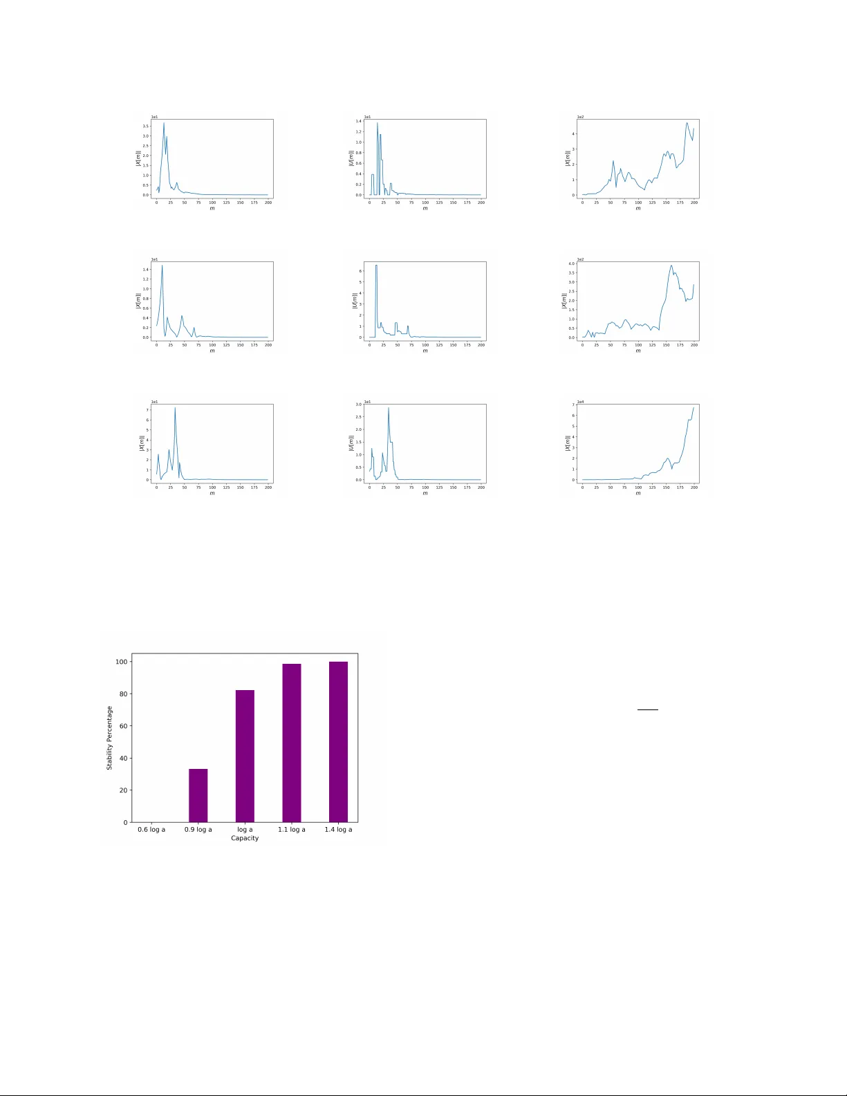
1 Stabilizing a linear system using phone calls: when time is inf ormation Mohammad Jav ad Khojasteh, Massimo Franceschetti, Gireeja Ranade Abstract —W e consider the problem of stabilizing an undis- turbed, scalar , linear system o ver a “timing” channel, namely a channel where information is communicated through the timestamps of the transmitted symbols. Each symbol transmitted from a sensor to a controller in a closed-loop system is received subject to some to random delay . The sensor can encode messages in the waiting times between successive transmissions and the controller must decode them from the inter-r eception times of successive symbols. This set-up is analogous to a telephone system where a transmitter signals a phone call to a receiver thr ough a “ring” and, after the random delay required to establish the connection; the recei ver is aware of the “ring” being recei ved. Since there is no data payload exchange between the sensor and the controller , this set-up provides an abstraction for performing event-triggering control with zero-payload rate. W e show the follo wing requirement for stabilization: f or the state of the system to conv erge to zero in probability , the timing capacity of the channel should be, essentially , at least as large as the entropy rate of the system. Con versely , in the case the symbol delays are exponentially distributed, we show an “almost” tight sufﬁcient condition using a coding strategy that reﬁnes the estimate of the decoded message every time a new symbol is recei ved. Our r esults generalize pre vious zero-payload event-triggering control strategies, revealing a fundamental limit in using timing information for stabilization, independent of any transmission strategy . Index T erms —T iming channel, control with communication constraints, ev ent-triggered control, linear systems. I . I N T RO D U C T I O N A networked control system with a feedback loop over a communication channel provides a ﬁrst-order approximation of a cyber-ph ysical system (CPS), where the interplay between the communication and control aspects of the system leads to new and unexpected analysis and design challenges [3], [4]. In this setting, data-rate theorems quantify the impact of the communication channel on the ability to stabilize the system. Roughly speaking, these theorems state that stabilization re- quires a communication rate in the feedback loop at least as large as the intrinsic entropy rate of the system, expressed by the sum of the logarithms of its unstable eigenv alues [5]–[12]. W e consider a speciﬁc communication channel in the loop — a timing c hannel . Here, information is communicated The material in this paper was presented in part at the 18th European Control Conference (ECC), 2019 [1], and at 57th IEEE Conference on on Decision and Control, 2018 [2]. This research was partially supported by NSF awards CNS-1446891 and ECCS-1917177. M. J. Khojasteh is with the W ireless Communication and Network Sciences Laboratory (WINS Lab), Massachusetts Institute of T echnology . Some of this work was performed while at Uni versity of California, San Diego, and also visiting Microsoft Research. (mkhojast@mit.edu) M. Franceschetti is with the Department of Electrical and Computer Engineering, University of California, San Diego. (massimo@ucsd.edu) G. Ranade is with EECS department at the Univ ersity of California, Berkeley . Some of this work was performed while at Microsoft Re- search, and also at the Simons Institute for the Theory of Computing. (gireeja@eecs.berkeley .edu) through the timestamps of the symbols transmitted over the channel; the time is carrying the message. This formulation is motiv ated by recent works in e vent-triggering control, sho wing that the timing of the triggering ev ents carries information that can be used for stabilization [13]–[20]. By encoding informa- tion in timing, stabilization can be achieved by transmitting additional data at a rate arbitrarily close to zero. Howe ver , in these works, the timing information was not explicitly quanti- ﬁed, and the analysis was limited to speciﬁc e vent-triggering strategies. In this paper , our goal is to determine the value of a timestamp from an information-theoretic perspectiv e, when this timestamp is used for control. W e are further motiv ated by the results on the impact of multiplicati ve noise in control [21], [22], since timing uncertainty can lead to multiplicativ e noise in systems and thus can serve as an information bottleneck. T o illustrate the proof of concept that timing carries in- formation useful for control, we consider the simple case of stabilization of a scalar , undisturbed, continuous-time, un- stable, linear system over a timing channel and rely on the information-theoretic notion of timing capacity of the chan- nel, namely the amount of information that can be encoded using time stamps [23]–[39]. In this setting, the sensor can communicate with the controller by choosing the timestamps at which symbols from a unitary alphabet are transmitted. The controller receives each transmitted symbol after a random delay is added to the timestamp. W e show the follo wing data- rate theorem. For the state to con verge to zero in probability , the timing capacity of the channel should be, essentially , at least as large as the entropy rate of the system. Con v ersely , in the case the random delays are exponentially distributed, we show that when the timing capacity is strictly greater than the entropy rate of the system, we can drive the state to zero in probability by using a decoder that reﬁnes its estimate of the transmitted message every time a new symbol is recei ved [40]. W e also derive analogous necessary and suf ﬁcient conditions for the problem of estimating the state of the system with an error that tends to zero in probability . The books [5], [6], [50], [51] and the surve ys [7], [8], [52] provide detailed discussions of data-rate theorems and related results that heavily inspire this work. A portion of the literature studied stabilization over “bit-pipe channels, ” where a rate-limited, possibly time-varying and erasure-prone communication channel is present in the feedback loop [41], [46]–[48], [53]. For more general noisy channels, T atikonda and Mitter [42] and Matvee v and Sa vkin [43] showed that the state of undisturbed linear systems can be forced to conv erge to zero almost surely (a.s.) if and only if the Shannon capacity of the channel is larger than the entropy rate of the system. In the presence of disturbances, in order to keep the state bounded a.s., a more stringent condition is required, namely the zero-error capacity of the channel must be larger than 2 T ABLE I: Capacity notions used to derive data-rate theorems in the literature under dif ferent notions of stability , channel types, and system disturbances. W ork Disturbance Channel Stability condition Capacity [41] NO Bit-pipe | X ( t ) | → 0 a.s. Shannon [42], [43] NO DMC | X ( t ) | → 0 a.s. Shannon [44] bounded DMC P (sup t | X ( t ) | < ∞ ) = 1 Zero-Error [6, Ch. 8] bounded DMC P (sup t | X ( t ) | < K  ) > 1 −  Shannon [45] bounded DMC sup t E ( | X ( t ) | m ) < ∞ Anytime [46] unbounded Bit-Pipe sup t E ( | X ( t ) | 2 ) < ∞ Shannon [47]–[49] unbounded V ar . Bit-pipe sup t E ( | X ( t ) | m ) < ∞ Anytime This paper NO T iming | X ( t ) | P → 0 T iming the entropy rate of the system [44]. Nair deriv ed a similar information-theoretic result in a non-stochastic setting [54]. Sahai and Mitter [45] considered moment-stabilization ov er noisy channels and in the presence of system disturbances of bounded support, and provided a data-rate theorem in terms of the anytime capacity of the channel. They showed that to keep the m th moment of the state bounded, the anytime capacity of order m should be larger than the entropy rate of the system. The an ytime capacity has been further inv estigated in [49], [55]–[57]. Matvee v and Savkin [6, Chapter 8] have also introduced a weaker notion of stability in probability , requiring the state to be bounded with probability (1 −  ) by a constant that div erges as  → 0 , and sho wed that in this case it is possible to stabilize linear systems with bounded disturbances over noisy channels provided that the Shannon capacity of the channel is larger than the entropy rate of the system. The various results, along with our contribution, are summarized in T able I. The main point that can be drawn from all of these results is that the relev ant capacity notion for stabilization over a communication channel critically depends on the notion of stability and on the system’ s model. From the system’ s perspective, our set-up is closest to the one in [41]–[43], as there are no disturbances and the objective is to driv e the state to zero. Our conv ergence in probability provides a stronger necessary condition for stabilization, but a weaker sufﬁcient condition than the one in these works. W e also point out that our notion of stability is considerably stronger than the notion of probabilistic stability proposed in [6, Chapter 8]. Some additional works considered nonlinear plants without disturbances [58]–[60], and switched linear systems [61], [62] where communication between the sensor and the controller occurs over a bit-pipe communication chan- nel. The recent work in [63] studies estimation of nonlinear systems ov er noisy communication channels and the work in [64] inv estigates the trade-offs between the communication channel rate and the cost of the linear quadratic regulator for linear plants. Parallel work in control theory has in v estigated the possibil- ity of stabilizing linear systems using timing information. One primary focus of the emerging paradigm of event-triggered control [65]–[77] has been on minimizing the number of transmissions while simultaneously ensuring the control ob- jectiv e [16], [78], [79]. Rather than performing periodic com- munication between the system and the controller , in ev ent- triggered control communication occurs only as needed, in an opportunistic manner . In this setting, the timing of the triggering events can carry useful information about the state of the system, that can be used for stabilization [13]–[20]. In this context, it has been shown that the amount of timing information is sensitive to the delay in the communication channel. While for small delay stabilization can be achiev ed using only timing information and transmitting data payload (i.e. physical data) at a rate arbitrarily close to zero, for large values of the delay this is not the case, and the data payload rate must be increased [15], [19]. In this paper , we extend these results from an information-theoretic perspecti ve, as we explicitly quantify the value of the timing information, independent of any transmission strategy . T o quantify the amount of timing information alone, we restrict to transmitting symbols from a unitary alphabet, i.e. at zero data payload rate. Research directions left open for future in vestigation include the study of “mixed” strategies, using both timing information and physical data transmitted ov er a larger alphabet, as well as generalizations to vector systems and the study of systems with disturbances. In the latter case, it is likely that the usage of stronger notions of capacity , or weaker notions of stability , will be necessary . The rest of the paper is organized as follows. Section II introduces the system and channels models. The main re- sults are presented in Section III. Section IV considers the estimation problem, and Section V considers the stabilization problem. Section VI provides a comparison with related work, and Section VII presents a numerical e xample. Conclusions are drawn in Section VIII. A. Notation Let X n = ( X 1 , · · · , X n ) denote a vector of random variables and let x n = ( x 1 , · · · , x n ) denote its realization. If X 1 , · · · , X n are independent and identically distributed (i.i.d) random variables, then we refer to a generic X i ∈ X n by X and skip the subscript i . W e use log and ln to denote the logarithms base 2 and base e respecti vely . W e use H ( X ) to denote the Shannon entropy of a discrete random v ariable X and h ( X ) to denote the differential entropy of a continuous random variable X . Further, we use I ( X ; Y ) to indicate the mutual information between random variables X and Y . W e 3 Fig. 1: Model of a networked control system where the feedback loop is closed over a timing channel. write X n P − → X if X n con ver ges in probability to X . Similarly , we write X n a.s. − − → X if X n con ver ges almost surely to X . For any set X and an y n ∈ N we let π n : X N → X n (1) be the truncation operator , namely the projection of a sequence in X N into its ﬁrst n symbols. I I . S Y S T E M A N D C H A N N E L M O D E L W e consider the network ed control system depicted in Fig. 1. The system dynamics are described by a scalar , continuous-time, noiseless, linear time-in v ariant (L TI) system ˙ X ( t ) = aX ( t ) + bU ( t ) , (2) where X ( t ) ∈ R and U ( t ) ∈ R are the system state and the control input respectiv ely . The constants a, b ∈ R are such that a > 0 and b 6 = 0 . The initial state X (0) is random and is drawn from a distribution of bounded differential entropy and bounded support, namely h ( X (0)) < ∞ and | X (0) | < L , where L is known to both the sensor and the controller . Conditioned on the realization of X (0) , the system e volution is deterministic. Both controller and sensor hav e knowledge of the system dynamics in (2). W e assume the sensor can measure the state of the system with inﬁnite precision, and the controller can apply the control input to the system with inﬁnite precision and with zero delay . The sensor is connected to the controller through a timing channel (the telephone signaling channel deﬁned in [23]). The operation of this channel is analogous to that of a telephone system where a transmitter signals a phone call to the recei ver through a “ring” and, after a random time required to establish the connection, is aw are of the “ring” being receiv ed. Com- munication between transmitter and receiver can then occur without any vocal exchange, b ut by encoding messages in the “waiting times” between consecutive calls. A. The channel W e model the channel as carrying symbols ♠ from a unitary alphabet, and each transmission is receiv ed after a random delay . Ev ery time a symbol is receiv ed, the sender is notiﬁed of the reception by an instantaneous acknowledgment. The channel is initialized with a ♠ received at time t = 0 . After receiving the ackno wledgment for the i th ♠ , the sender waits for W i +1 seconds and then transmits the next ♠ . Transmitted symbols are subject to i.i.d. random delays { S i } . Letting D i be the inter-reception time between two consecuti ve symbols, we hav e D i = W i + S i . (3) It follows that the reception time of the n th symbol is T n = n X i =1 D i . (4) Fig. 2 provides an example of the timing channel in action. B. Capacity of the c hannel W e start by revie wing some deﬁnitions from [23]. Deﬁnition 1: A ( n, M , T , δ ) -timing code for the telephone signaling channel consists of a codebook of M codew ords { ( w i,m , i = 1 , . . . , n ) , m = 1 . . . M } , as well as a decoder , which upon observation of ( D 1 , . . . , D n ) selects the correct transmitted codeword with probability at least 1 − δ . Moreov er , the codebook is such that the expected random arri val time of the n th symbol is at most T , namely E ( T n ) ≤ T . (5) Deﬁnition 2: The rate of an ( n, M , T , δ ) -timing code is R = (log M ) /T . (6) Deﬁnition 3: The timing capacity C of the telephone sig- naling channel is the supremum of the achie v able rates, namely the largest R such that for e very γ > 0 there exists a sequence of ( n, M n , T n , δ T n ) -timing codes that satisfy log M n T n > R − γ , (7) and δ T n → 0 as n → ∞ . The follo wing result [23, Theorem 8] characterizes the capacity of the telephone signaling channel. Theor em 1 (Ananthar am and V er dú): The timing capacity of the telephone signaling channel is giv en by C = sup χ> 0 sup W ≥ 0 E ( W ) ≤ χ I ( W ; W + S ) E ( S ) + χ , (8) and if S is exponentially distributed then C = 1 e E ( S ) [nats/sec]. (9) In this paper , we assume that the waiting times { W i } used to encode any gi ven message are generated at random in an i.i.d. fashion, and are also independent of the random delays { S i } . Assuming the symbols in each code word are pick ed i.i.d. from a common distribution restricts the encoder to using a ﬁxed random telephoning policy . This assumption comes at no loss of generality since: (i) the capacity in (8) is achiev ed by i.i.d. random codes [23], and (ii) in our system model there are no disturbances and therefore the control problem reduces to the communication of a ﬁxed real-v alued variable representing the initial condition with exponential reliability ov er a digital channel, which can be performed optimally using a ﬁxed random coding strategy [40]. 4 C. The sensor The sensor in Fig. 1 can act as a source and channel encoder . Based on its source knowledge, namely the knowledge of the initial condition X (0) , system dynamics (2), and L , it selects the waiting times { W i } between the reception and the transmission of consecutive ♠ symbols. As in [23], [26] we assume that the causal ackno wledgments receiv ed by the sensor every time a ♠ is delivered to the controller are not used to choose the w aiting times, but only to av oid queuing, ensuring that every symbol is sent after the previous one has been receiv ed. This applies to TCP-based networks, where packet deli veries are acknowledged via a feedback link [80]–[84]. For networked control systems, this causal ackno wledgment can be obtained without assuming an additional communication channel in the feedback loop. The controller can signal the ackno wledgment to the sensor by applying a control input to the system that e xcites a speciﬁc frequency of the state each time a symbol has been receiv ed. This strategy is kno wn in the literature as “ackno wledgment through the control input” [6], [13], [42], [45]. D. The contr oller The controller in Fig. 1 can act as a source and channel decoder . It uses the reception times of all the symbols recei ved up to time t , along with the knowledge of L and of the system dynamics (2) to decode the source message, compute the control input U ( t ) , and apply it to the system. The control input can be reﬁned ov er time, as the estimate of the source can be decoded with increasing accuracy when more and more symbols are recei ved. The objective is to design an encoding and decoding strategy to stabilize the system by driving the state to zero in probability , i.e. we want | X ( t ) | P − → 0 as t → ∞ . Although the computational complexity of different encoding-decoding schemes is a key practical issue, in this pa- per we are concerned with the existence of schemes satisfying our objecti ve, rather than with their practical implementation. I I I . M A I N R E S U LT S A. Necessary condition T o deri ve a necessary condition for the stabilization of the feedback loop system depicted in Fig. 1, we ﬁrst consider the problem of estimating the state in open-loop ov er the timing channel along a speciﬁc sequence of estimation times. W e show that if the estimation error tends to zero in probability along this sequence, then for all ν > 0 the timing capacity must be at least as large as (1 − ν ) times the entry rate of the system. This result holds for any source and random channel coding strate gies adopted by the sensor , and for any strategy adopted by the controller to generate the control input. Our proof employs a rate-distortion argument to compute a lower bound on the minimum number of bits required to represent the state up to any gi ven accuracy , and this leads to a corresponding lower bound on the required timing capacity of the channel. W e then sho w that the same bound on the timing capacity holds for stabilization, since in order to have | X ( t ) | P − → 0 as t → ∞ in closed-loop, the estimation error in open-loop must tend to zero in probability as t → ∞ , and therefore, in particular , along the designed sequence of estimation times. B. Sufﬁcient condition T o deriv e a sufﬁcient condition for stabilization, we ﬁrst consider the problem of estimating the state in open-loop ov er the timing channel. W e focus on a speciﬁc sequence of estimation times. W e provide an explicit source-channel coding scheme which guarantees that if for all ν > 0 the timing capacity is larger than (1 + ν ) times the entropy entropy rate of the system, then the estimation error tends to zero in probability . W e then show that this condition is also sufﬁcient to construct a control scheme such that | X ( t ) | P − → 0 as t → ∞ . The main idea behind our strategy is based on the realization that in the absence of disturbances all that is needed to dri ve the state to zero is communicating the initial condition X (0) to the controller with accuracy that increases e xponentially over time. Once this is achie ved, the controller can estimate the state X ( t ) with increasing accuracy ov er time, and continuously apply an input that driv es the state to zero. This idea has been exploited before in the literature [41], [42], and the problem is related to the anytime reliable transmission of a real-valued variable o ver a digital channel [40]. Here, we cast this problem in the framework of the timing channel. A main dif ﬁculty in our case is to ensure that we can driv e the system’ s state to zero in probability despite the unbounded random delays occurring in the timing channel. In the source coding process, we quantize the interval [ − L, L ] uniformly using a tree-structured quantizer [85]. W e then map the obtained source code into a channel code suitable for transmission over the timing channel, using the capacity- achieving random codebook of [23]. Gi ven X (0) , the encoder picks a code word from an arbitrarily lar ge codebook and starts transmitting the real numbers of the codew ord one by one, where each real number corresponds to a holding time, and proceeds in this way forev er . Every time a sufﬁciently large number of symbols are received, we use a maximum likelihood decoder to successiv ely reﬁne the controller’ s estimate of X (0) . Namely , the controller re-estimates X (0) based on the ne w inter -reception times and all pre vious inter-reception times, and uses it to compute the new state estimate of X ( t ) and control input U ( t ) . W e show that when the sensor quantizes X (0) at sufﬁciently high resolution, and when the timing capacity is larger than the entrop y rate of the system, the controller can construct a sufﬁciently accurate estimate of X ( t ) and compute U ( t ) such that | X ( t ) | P − → 0 as t → ∞ . I V . T H E E S T I M A T I O N P RO B L E M W e start considering the estimation problem depicted in Fig. 3. By letting b = 0 in (2) we obtain the open-loop equation ˙ X e ( t ) = aX e ( t ) . (10) W e assume that the encoder has causal knowledge of the reception times via acknowledgments through the system as depicted in Fig. 3. Our ﬁrst objectiv e is to obtain a necessary condition on the capacity of the timing channel required to 5 Fig. 2: The timing channel. Subscripts s and r are used to denote sent and receiv ed symbols, respectiv ely . Fig. 3: The estimation problem. construct an estimate ˆ X e ( t n ) such that for all ν > 0 and any sequence of estimation times t n that satisﬁes 1 − ν ≤ lim n →∞ t n E ( T n ) < 1 , (11) we hav e | X e ( t n ) − ˆ X e ( t n ) | P → 0 as n → ∞ . Our second objecti ve is to obtain a sufﬁcient condition on the capacity of the timing channel that ensures the construction of an estimate ˆ X e ( t 0 n ) such that for all ν > 0 and any sequence of estimation times t 0 n that satisﬁes 1 < lim n →∞ t 0 n E ( T n ) ≤ 1 + ν, (12) we hav e | X e ( t 0 n ) − ˆ X e ( t 0 n ) | P → 0 as n → ∞ . The sequences of estimation times that satisfy (11) and (12) are “close” in the sense that lim n →∞ t 0 n − t n E ( T n ) ≤ 2 ν. (13) Giv en the conditions in (11) and (12), the next lemma provides probabilistic bounds on the number of symbols that are receiv ed up to time t n and t 0 n , respectiv ely . Lemma 1: Giv en the conditions in (11), the probability P ( T n +1 ≤ t n ) tends to zero. Moreover , gi ven the condition in (12), as n → ∞ , the probability P ( T n > t 0 n ) tends to zero. Pr oof: W e start by proving that P ( T n +1 ≤ t n ) tends to zero as n → ∞ . For large enough n , using (11), we hav e that the probability of recei ving the n + 1 symbols before t n is P ( T n +1 ≤ t n ) ≤ P ( T n +1 / ( n + 1) < E ( T n ) / ( n + 1)) ≤ P ( T n +1 / ( n + 1) < E ( D )) . (14) Since the waiting times { W i } and the random delays { S i } are i.i.d. sequences and independent of each other , it follo ws by the strong la w of large numbers that (14) tends to zero as n → ∞ . W e continue by bounding the probability of the event that the n -th symbol does not arri ve by the estimation deadline t 0 n . For lar ge enough n , using (12), we hav e that the probability of missing the deadline is P ( T n > t 0 n ) ≤ P ( T n /n > E ( T n ) /n ) = P ( T n /n > E ( D )) . (15) Since the waiting times { W i } and the random delays { S i } are i.i.d. sequences and independent of each other , it follo ws by the strong la w of large numbers that (15) tends to zero as n → ∞ . Lemma 1 leads to the follo wing conclusions. First, with high probability as n → ∞ , by time t n at most n symbols have been receiv ed. Second, with high probability as n → ∞ the estimation at time t 0 n is ev aluated, after at least n symbols hav e been recei ved. A. Necessary condition The next theorem provides a necessary condition on the timing capacity for the state estimation error to tend to zero in probability . Theor em 2: Consider the estimation problem depicted in Fig. 3 with system dynamics (10). Consider transmit- ting n symbols ov er the telephone signaling channel (3), and the sequence of estimation times satisfying (11). If | X e ( t n ) − ˆ X e ( t n ) | P → 0 , then I ( W ; W + S ) ≥ a (1 − ν ) E ( W + S ) [ nats ] , (16) and consequently C ≥ a (1 − ν ) [ nats / sec ] . (17) The proof of Theorem 2 is giv en in the appendix. B. Sufﬁcient condition The next theorem provides a sufﬁcient condition for con- ver gence of the state estimation error to zero in probability along any sequence of estimation times t 0 n satisfying (12), in the case of e xponentially distributed delays. Theor em 3: Consider the estimation problem depicted in Fig. 3 with system dynamics (10). Consider transmitting n symbols over the telephone signaling channel (3). Assume { S i } are drawn i.i.d. from exponential distribution with mean E ( S ) . If the capacity of the timing channel is at least C ≥ a (1 + ν ) [ nats / sec ] , (18) 6 then for any sequence of times { t 0 n } that satisﬁes (12), we can compute an estimate ˆ X e ( t 0 n ) such that as n → ∞ , we ha ve | X e ( t 0 n ) − ˆ X e ( t 0 n ) | P → 0 . (19) The proof of Theorem 3 is giv en in the appendix. The result is strengthened in the next section (see Corollary 1), showing that C > a (1 + ν ) is also sufﬁcient to dri ve the state estimation error to zero in probability for all t → ∞ . Remark 1: Since ν > 0 can be chosen to be sufﬁciently small Theorems 2 and 3 provide an “almost" tight neces- sary and sufﬁcient condition for the estimation problem. The entropy-rate of our system is a nats/time [58], [86]–[89]. This represents the amount of uncertainty per unit time generated by the system in open loop. In fact, (16), can be seen as a typical scenario in data-rate theorems: to driv e the error to zero the mutual information between an encoding symbol W and its receiv ed noisy version W + S should be larger than the a verage “information growth” of the state during the inter - reception interval D , which is giv en by E ( aD ) = a E ( W + S ) . (20) • V . T H E S T A B I L I Z A T I O N P RO B L E M A. Necessary condition W e no w turn to consider the stabilization problem. Our ﬁrst lemma states that if in closed-loop we are able to driv e the state to zero in probability , then in open-loop we are also able to estimate the state with vanishing error in probability . Lemma 2: Consider stabilization of the closed-loop sys- tem (2) and estimation of the open-loop system (10) over the timing channel (3). If there exists a controller such that | X ( t ) | P → 0 as t → ∞ , in closed-loop, then there exists an estimator such that | X e ( t ) − ˆ X e ( t ) | P → 0 as t → ∞ , in open- loop. Pr oof: From (2), we have in closed loop X ( t ) = e at X (0) + ζ ( t ) , (21) ζ ( t ) = e at Z t 0 e − a% bU ( % ) d%. (22) It follows that if lim t →∞ P ( | X ( t ) | ≤  ) = 1 , (23) then we also ha ve lim t →∞ P    e at X (0) + ζ ( t )   ≤   = 1 . (24) On the other hand, from (10) we have in open loop X e ( t ) = e at X (0) , (25) and we can choose ˆ X e ( t ) = − ζ ( t ) so that | X e ( t ) − ˆ X e ( t ) | = | e at X (0) + ζ ( t ) | P → 0 , (26) where the last step follo ws from (24). The next theorem provides a necessary rate for the stabi- lization problem. Theor em 4: Consider the stabilization of the closed-loop system (2). If | X ( t ) | P → 0 as t → ∞ , then I ( W ; W + S ) ≥ a (1 − ν ) E ( W + S ) [ nats ] , (27) and consequently C ≥ a (1 − ν ) [ nats / sec ] . (28) Pr oof: By Lemma 2 we have that if | X ( t ) | P → 0 , then | X e ( t ) − ˆ X e ( t ) | P → 0 for all t → ∞ , and in particular along a sequence { t n } satisfying (11). The result now follows from Theorem 2. B. Sufﬁcient condition Our next lemma strengthens our estimation results, stating that it is enough for the state estimation error to conv erge to zero in probability as n → ∞ along a sequence of estimation times { t 0 n } satisfying (12), to ensure it conv erges to zero for all t → ∞ . Lemma 3: Consider estimation of the system (10) ov er the timing channel (3). If there exists Γ 0 > 1 such that along the sequence of estimation times t 0 n = Γ 0 E ( T n ) we hav e | X e ( t 0 n ) − ˆ X e ( t 0 n ) | P → 0 as n → ∞ , then for all t → ∞ we also hav e | X e ( t ) − ˆ X e ( t ) | P → 0 . Pr oof: W e have that for t 0 n = Γ 0 E ( T n ) and for all  0 > 0 , and φ > 0 , there exist n φ such that for all n ≥ n φ P  | X e ( t 0 n ) − ˆ X e ( t 0 n ) | >  0  ≤ φ. (29) Let t n φ = Γ 0 E ( T n φ ) be the time at which we estimate the state for the n φ th time. W e want to show that for all t ∈ [ t n φ , t n φ +1 ] and  > 0 , we also have P  | X e ( t ) − ˆ X e ( t ) | >   ≤ φ. (30) Consider the random time T n φ at which ♠ is received for the n φ th time. W e have t n φ +1 − t n φ = Γ 0 E ( T n φ +1 ) − Γ 0 E ( T n φ ) = ( n φ + 1)Γ 0 E ( D ) − n φ Γ 0 E ( D ) = Γ 0 E ( D ) . (31) For all t ∈ [ t n φ , t n φ +1 ] , from the open-loop equation (10) we hav e X e ( t ) = e a ( t − t n φ ) X e ( t n φ ) . (32) W e then let ˆ X e ( t ) = e a ( t − t n φ ) ˆ X e ( t n φ ) . (33) Combining (32) and (33) and using (31), we obtain that for all t ∈ [ t n φ , t n φ +1 ] | X e ( t ) − ˆ X e ( t ) | ≤ e a Γ 0 E ( D ) | X e ( t n φ ) − ˆ X e ( t n φ ) | . (34) From which it follo ws that P  | X e ( t ) − ˆ X e ( t ) | >  0 e a Γ 0 E ( D )  ≤ P  | X e ( t n φ ) − ˆ X e ( t n φ ) | >  0  . (35) 7 Since (29) holds for all n ≥ n φ , we also ha ve P  | X e ( t n φ ) − ˆ X e ( t n φ ) | ≥  0  ≤ φ. (36) W e can now let  0 < e − a Γ 0 E ( D ) and the result follows. Lemma 3 yields the following corollary , which is an imme- diate extension of Theorem 3. Cor ollary 1: Consider the estimation problem depicted in Fig. 3 with system dynamics (10). Consider transmitting n symbols over the telephone signaling channel (3). Assume { S i } are drawn i.i.d. from exponential distribution with mean E ( S ) . If the capacity of the timing channel is at least C ≥ a (1 + ν ) , then we ha ve | X e ( t ) − ˆ X e ( t ) | P → 0 as t → ∞ . Pr oof: W e start by considering the sequence of estimation times t 0 n = (1 + ν ) E ( T n ) . Since C ≥ a (1 + ν ) , by Theorem 3 we hav e | X e ( t 0 n ) − ˆ X e ( t 0 n ) | P → 0 as n → ∞ . Then, by Lemma 3 we also ha ve | X e ( t ) − ˆ X e ( t ) | P → 0 as t → ∞ . The next ke y lemma states that if we are able to estimate the state with v anishing error in probability , then we are also able to drive the state to zero in probability . Lemma 4: Consider stabilization of the closed-loop sys- tem (2) and estimation of the open-loop system (10) over the timing channel (3). If there exists an estimator such that | X e ( t ) − ˆ X e ( t ) | P → 0 as t → ∞ , in open-loop, then there exists a controller such that | X ( t ) | P → 0 as t → ∞ , in closed- loop. Pr oof: W e start by showing that if there exists an open- loop estimator such that | X e ( t ) − ˆ X e ( t ) | P → 0 as t → ∞ , then there also exists a closed-loop estimator such that | X ( t ) − ˆ X ( t ) | P → 0 as t → ∞ . W e construct the closed-loop estimator based on the open-loop estimator as follows. The sensor in closed-loop runs a copy of the open-loop system by constructing the virtual open-loop dynamic X e ( t ) = X (0) e at . (37) Using the open-loop estimator, for all t > 0 the con- troller acquires the open-loop estimate ˆ X e ( t ) such that | X e ( t ) − ˆ X e ( t ) | P → 0 . It then uses this estimate to construct the closed-loop estimate ˆ X ( t ) = ˆ X e ( t ) + e at Z t 0 e − a% bU ( % ) d%. (38) Since from (2) the true state in closed loop is X ( t ) = X (0) e at + e at Z t 0 e − a% bU ( % ) d%, (39) it follows by combining (37), (38) and (39) that | X ( t ) − ˆ X ( t ) | = | X e ( t ) − ˆ X e ( t ) | P → 0 . (40) What remains to be proven is that if | X ( t ) − ˆ X ( t ) | P → 0 , then there exists a controller such that | X ( t ) | P → 0 . Let b > 0 and choose k so large that a − bk < 0 . Let U ( t ) = − k ˆ X ( t ) . From (2), we ha ve ˙ X ( t ) = ( a − bk ) X ( t ) + bk [ X ( t ) − ˆ X ( t )] . (41) By solving (41) and using the triangle inequality , we get | X ( t ) | ≤| e ( a − bk ) t X (0) | +     Z t 0 e ( t − % )( a − bk ) bk ( X ( % ) − ˆ X ( % )) d%     . (42) Since | X (0) | < L and a − bk < 0 , the ﬁrst term in (42) tends to zero as t → ∞ . Namely , for any  > 0 there exists a number N  such that for all t ≥ N  , we have | e ( a − bk ) t X (0) | ≤ . (43) Since by (40) we hav e that | X ( t ) − ˆ X ( t ) | P → 0 , we also have that for any , δ > 0 there exist a number N 0  such that for all t ≥ N 0  , we have P  | X ( t ) − ˆ X ( t ) | ≤   ≥ 1 − δ . (44) It now follows from (42) that for all t ≥ max { N  , N 0  } the following inequality holds with probability at least (1 − δ ) | X ( t ) | ≤  + bk e t ( a − bk ) Z N 0  0 e − % ( a − bk ) | X ( % ) − ˆ X ( % ) | d% + bk e t ( a − bk ) Z t N 0  e − % ( a − bk ) d%. (45) Since both sensor and controller are a ware that | X (0) | < L , by (37) we have that for all t ≥ 0 the open-loop estimate acquired by the controller satisﬁes ˆ X e ( t ) ∈ [ − Le at , Le at ] . By (40) the closed-loop estimation error is the same as the open-loop estimation error , and we then hav e that for all % ∈ [0 , N 0  ] | X ( % ) − ˆ X ( % ) | = | X e ( % ) − ˆ X e ( % ) | ≤ 2 Le aN 0  . (46) Substituting (46) into (45), we obtain that with probability at least (1 − δ ) | X ( t ) | ≤  + 2 Lbk e [ t ( a − bk )+ aN 0  ] e − N 0  ( a − bk ) − 1 − ( a − bk ) + bk e t ( a − bk ) e − t ( a − bk ) − e − N 0  ( a − bk ) − ( a − bk ) . (47) By ﬁrst letting  be sufﬁciently close to zero, and then letting t be sufﬁciently large, we can make the right-hand side of (47) arbitrarily small, and the result follows. The next theorem combines the results above, pro viding a sufﬁcient condition for conv ergence of the state to zero in probability in the case of exponentially distributed delays. Theor em 5: Consider the stabilization of the system (2). Assume { S i } are dra wn i.i.d. from an exponential distrib ution with mean E ( S ) . If the capacity of the timing channel is at least C ≥ a (1 + ν ) [ nats / sec ] , (48) then | X ( t ) | P → 0 as t → ∞ . V I . C O M PA R I S O N W I T H P R E V I O U S W O R K A. Comparison with stabilization o ver an erasur e channel In [42] the problem of stabilization of the discrete-time version of the system in (2) ov er an erasure channel has been considered. In this discrete model, at each time step of the 8 system’ s e volution the sensor transmits I bits to the controller and these bits are successfully delivered with probability 1 − µ , or they are dropped with probability µ , in an independent fashion. It is sho wn that a necessary condition for X ( k ) a.s − − → 0 is that the capacity of this I -bit erasure channel is (1 − µ ) I ≥ log a [ bits / sec ] . (49) Since almost sure con vergence implies con vergence in prob- ability , by Theorem 4 we have that the following necessary condition holds in our setting for X ( t ) a.s. − − → 0 : I ( W ; W + S ) E ( W + S ) ≥ a (1 − ν ) [ nats/sec ] , (50) where ν > 0 can be arbitrarily small. W e now compare (49) and (50). The rate of expansion of the state space of the continuous system in open loop is a nats per unit time, while for the discrete system is log a bits per unit time. Accordingly , (49) and (50) are parallel to each other: in the case of (50) the controller must receiv e at least a E ( W + S ) nats representing the initial state during a time interval of av erage length E ( W + S ) . In the case of (49) the controller must recei ve at least log a/ (1 − µ ) bits representing the initial state ov er a time interval whose average length corresponds to the average number of trials before the ﬁrst successful reception (1 − µ ) ∞ X k =0 ( k + 1) µ k = 1 1 − µ . (51) B. Comparison with event triggering strate gies The works [13]–[20] use ev ent-triggering strategies that exploit timing information for stabilization ov er a digital communication channel. These strategies encode information ov er time in a speciﬁc state-dependent fashion and use a combination of timing information and data payload to con v ey information used for stabilization. Our framework, by considering the transmission of symbols from a unitary alphabet, uses only timing information for stabilization. In Theorem 4 we provide a fundamental limit on the rate at which information can be encoded in time, independent of any transmission strategy . Theorem 5 then shows that this limit can be almost achiev ed, in the case of exponentially distrib uted delays. The work [14] sho ws that using e vent triggering it is possible to achieve stabilization with any positive transmission rate ov er a zero-delay digital communication channel. Indeed, for channels without delay achieving stabilization at zero rate is easy . One could for example transmit a single symbol at a time equal to any bijective mapping of x (0) into a point of the non-negati ve reals. For example, we could transmit ♠ at time t = tan − 1 ( x (0)) for t ∈ [0 , π ] . The reception of the symbol would rev eal the initial state exactly , and the system could be stabilized. The work in [15] shows that when the delay is positi ve, b ut sufﬁciently small, a triggering policy can still achieve stabi- lization with any positi ve transmission rate. Howe ver , as the delay increases past a critical threshold, the timing information becomes so much out-of-date that the transmission rate must begin to increase. In our case, since the capacity of our timing channel depends on the distribution of the delay , we may also expect that a large v alue of the capacity , corresponding to a small av erage delay , would allow for stabilization to occur using only timing information. Indeed, when delays are distributed e xponentially , from (9) and Theorem 5 it follows that as longs as the expected v alue of delay is E ( S ) < 1 e a , (52) it is possible to stabilize the system by using only timing information. On the other hand, the system is not stabilizable using only timing information if the expected value of the delay becomes larger than ( e a ) − 1 . V I I . N U M E R I C A L E X A M P L E W e now present a numerical simulation of stabilization ov er the telephone signaling channel. While our analysis is for continuous-time systems, the simulation is performed in discrete time, considering the system X [ m ] = aX [ m ] + U [ m ] , for m ∈ N , (53) where a > 1 so that the system is unstable. In this case, assuming i.i.d. geometrically distributed delays { S i } , the sufﬁcient condition for stabilization becomes C ≥ log a (1 + ν ) [ nats / sec ] , (54) where C is the timing capacity of the discrete telephone signaling channel [24]. The timing capacity is achiev ed in this case using i.i.d. waiting times { W i } that are distrib uted according to a mixture of a geometric and a delta distrib ution. This results in { D i } also being i.i.d. geometric [24], [26]. Assuming that a decoding operation occurs at time m using all k m symbols receiv ed up to this time, and following the source-channel coding scheme described in the proof of Theorem 3, the controller decodes an estimate ˆ X m [0] of the initial state and estimates the current state as ˆ X [ m ] = a m ˆ X m [0] + m − 1 X j =0 a m − 1 − j U [ j ] . (55) The estimate ˆ X m [0] corresponds to the binary representation of X (0) using d k m E ( D ) C e bits, provided that there is no decoding error in the tranmsission. Accordingly , in our sim- ulation, we let η > 0 and P e = e − η k m , and we assume that at every decoding time, with probability (1 − P e ) we construct a correct quantized estimate of the initial state ˆ X m [0] using d k m E ( D ) C e bits. Alternati vely , with probability P e we construct an incorrect quantized estimate. In the case of a correct estimate, we apply the asymptotically optimal control input U [ m ] = − K ˆ X [ m ] , where K > 0 is the control gain and ˆ X [ m ] is obtained from (55). In the case of an incorrect estimate, the state estimate used to construct the control input can be arbitrary . W e consider three cases: (i) we do not apply any control input and let the system ev olve in open loop, (ii) we apply the control input using the previous estimate, (iii) we apply the opposite of the asymptotically optimal control input: U [ m ] = K ˆ X [ m ] . In all cases, the control input remains ﬁxed to its most recent v alue during the time required for a new estimate to be performed. 9 Fig. 4: Ev olution of the channel used in the simulation in an error-free case. Each time ♠ is receiv ed, a ne w codeword is decoded using all the symbols receiv ed up to that time. The decoded codew ord represents the initial state X [0] with a precision that increases by E ( D ) C bits at each symbol reception. In the ﬁgure, for illustration purposes we have assumed E ( D ) C = 3 bits. Fig. 4 pictorially illustrates the ev olution of our simulation in an error-free case in which the binary representation of X [0] is reﬁned by E ( D ) C = 3 bits at each symbol reception. Numerical results are depicted in Fig. 5, showing conv er- gence of the state to zero in all cases, provided that the timing capacity is above the entropy rate of the system. In contrast, when the timing capacity is below the entropy rate, the state div erges. The plots also sho w the absolute v alue of the control input used for stabilization in the various cases. Fig. 6 illustrates the percentage of times at which the controller successfully stabilized the plant versus the capacity of the channel in a run of 500 Monte Carlo simulations. The phase transition behavior at the critical value C = log a is clearly evident. V I I I . C O N C L U S I O N S In the framework of control of dynamical systems over communication channels, it has recently been observed that ev ent-triggering policies encoding information over time in a state-dependent fashion can exploit timing information for stabilization in addition to the information traditionally carried by data packets [13]–[20]. In a more general framew ork, this paper studied from an information-theoretic perspectiv e the fundamental limitation of using only timing information for stabilization, independent of any transmission strategy . W e showed that for stabilization of an undisturbed scalar linear system ov er a channel with a unitary alphabet, the timing capacity [23] should be, essentially , at least as large as the entropy rate of the system. In addition, in the case of exponentially distributed delays, we provided an almost tight sufﬁcient condition using a coding strategy that reﬁnes the estimate of the decoded message as more and more symbols are received. Important open problems for future research include the effect of system disturbances, understanding the combination of timing information and packets with data payload, and extensions to vector systems. Our deriv ation ensures that when the timing capacity is larger than the entropy rate, the estimation error does not gro w unbounded, in probability , e ven in the presence of the random delays occurring in the timing channel. This is made possible by communicating a real-valued v ariable (the initial state) at an increasingly higher resolution and with vanishing probability of error . This strate gy has been pre viously studied in [40] in the context of estimation over the binary erasure channel, rather than over the timing channel. It is also related to communica- tion at increasing resolution o ver channels with feedback via posterior matching [90], [91]. The classic Horstein [92] and Schalkwijk-Kailath [93] schemes are special cases of posterior matching for the binary symmetric channel and the additive Gaussian channel respectively . The main idea in our setting is to employ a tree-structured quantizer in conjunction to a capacity-achieving timing channel codebook that gro ws expo- nentially with the tree depth, and re-compute the estimate of the real-valued v ariable as more and more channel symbols are receiv ed. The estimate is re-computed for a number of recei ved symbols that depends on the channel rate and on the a verage delay . In contrast to posterior matching, we are not concerned with the complexity of the encoding-decoding strategy , but only with its existence. W e also do not assume a speciﬁc distribution for the real v alue we need to communicate, and we do not use the feedback signal to perform encoding, but only to a void queuing [23], [26]. W e point out that our control strategy does not w ork in the presence of disturbances: in this case, one needs to track a state that depends not only on the initial condition, but also on the evolution of the disturbance. This requires to update the entire history of the system’ s states at each symbol reception [45], leading to a different, i.e. non- classical, coding model. Alternati vely , remaining in a classical setting one could aim for less, and attempt to obtain results using weak er probabilistic notions of stability , such as the one in [6, Chapter 8]. Finally , by showing that in the case of no disturbances and exponentially distributed delay it is possible to achiev e stabi- lization at zero data-rate only for sufﬁciently small av erage delay E ( S ) < ( e a ) − 1 , we conﬁrmed from an information- theoretic perspecti ve the observation made in [15] regarding the existence of a critical delay value for stabilization at zero data-rate. A P P E N D I X A. Pr oof of Theorem 2 W e start by introducing a few deﬁnitions and proving some useful lemmas. Deﬁnition 4: For any  > 0 and φ > 0 , we deﬁne the rate- distortion function of the source ˙ X e = aX e ( t ) at times { t n } as R  t n ( φ ) = inf P ( ˆ X e ( t n ) | X e ( t n ) ) ( I  X e ( t n ); ˆ X e ( t n )  : (56) 10 Case I: decoding error → open loop C = 1 . 2 log a C = 1 . 2 log a C = 0 . 9 log a Case II: decoding error → previous estimate C = 1 . 2 log a C = 1 . 2 log a C = 0 . 9 log a Case III: decoding error → opposite of the optimal control C = 1 . 2 log a C = 1 . 2 log a C = 0 . 9 log a Fig. 5: Here we show the evolution of a single run of a system with dif ferent capacities for the timing channel. The ﬁrst and second columns represent the absolute value of the state and control input, respecti vely , when the timing capacity is larger than the entropy rate of the system ( C > log a ) . The third column represents the absolute value of the state when the timing capacity is smaller than the entropy rate of the system ( C < log a ) . In the ﬁrst ro w , in the presence of a decoding error , we do not apply any control input and let the system evolv e in open-loop; in the second row , we apply the control using the previous estimate; the third ro w , we apply the opposite of the optimal control. The simulation parameters were chosen as follows: a = 1 . 2 , E ( D ) = 2 , and P e = e − ηk m , where η = 0 . 09 . For the optimal control gain we hav e chosen K = 0 . 4 , which is optimal with respect to the (time-averaged) linear quadratic regulator (LQR) control cost (1 / 200) E [ P 199 m =0 (0 . 01 X 2 k + 0 . 5 U 2 k ) + 0 . 01 X 2 200 ] . Fig. 6: Here we show the fraction of times stabilization was achieved versus the capacity of the channel across a run of 500 simulations for each value of the capacity . Successful stabilization is deﬁned in these simulations as | X [250] | ≤ 0 . 05 . In the case of a decoding error , no control input is applied and we let the system e volv e in open loop. The simulation parameters were chosen as follows: a = 1 . 2 , E ( D ) = 2 , P e = e − ηk m , where η = 0 . 09 , and the control gain is K = 0 . 4 . P  | X e ( t n ) − ˆ X e ( t n ) | >   ≤ φ ) . The proof of the following lemma adapts an argument of [42] to our continuous-time setting. Lemma 5: W e ha ve R  t n ( φ ) ≥ (1 − φ ) [ a t n + h ( X (0))] (57) − ln 2  − ln 2 2 [ nats ] . Pr oof: Let ξ =  0 if | X e ( t n ) − ˆ X e ( t n ) | ≤  1 if | X e ( t n ) − ˆ X e ( t n ) | > . (58) Using the chain rule, we hav e I ( X e ( t n ); ˆ X e ( t n )) = I ( X e ( t n ); ξ , ˆ X e ( t n )) − I ( X e ( t n ); ξ | ˆ X e ( t n )) (59) = I ( X e ( t n ); ξ , ˆ X e ( t n )) − H ( ξ | ˆ X e ( t n )) + H ( ξ | X e ( t n ) , ˆ X e ( t n )) . Giv en X ( t n ) and ˆ X ( t n ) , there is no uncertainty in ξ , hence we deduce I ( X e ( t n ); ˆ X e ( t n )) = I ( X e ( t n ); ξ , ˆ X e ( t n )) − H ( ξ | ˆ X e ( t n )) = h ( X e ( t n )) − h ( X e ( t n ) | ξ , ˆ X e ( t n )) − H ( ξ | ˆ X e ( t n )) 11 = h ( X e ( t n )) − h ( X e ( t n ) | ξ = 0 , ˆ X e ( t n )) P ( ξ = 0) (60) − h ( X e ( t n ) | ξ = 1 , ˆ X e ( t n )) P ( ξ = 1) − H ( ξ | ˆ X e ( t n )) . Since H ( ξ | ˆ X e ( t n )) ≤ H ( ξ ) ≤ ln 2 / 2 [ nats ] , P ( ξ = 0) ≤ 1 , and P ( ξ = 1) ≤ φ , it then follows that I ( X e ( t n ); ˆ X e ( t n )) ≥ h ( X e ( t n )) − h  X e ( t n ) − ˆ X e ( t n ) | ξ = 0 , ˆ X e ( t n )  − h  X e ( t n ) | ξ = 1 , ˆ X e ( t n )  φ − ln 2 2 . (61) Since conditioning reduces the entropy , we ha ve I ( X e ( t n ); ˆ X e ( t n )) ≥ h ( X e ( t n )) (62) − h ( X e ( t n ) − ˆ X e ( t n ) | ξ = 0) − h ( X e ( t n )) φ − ln 2 2 = (1 − φ ) h ( X e ( t n )) − h ( X e ( t n ) − ˆ X e ( t n ) | ξ = 0) − ln 2 2 . By (58) and since the uniform distribution maximizes the differential entropy among all distributions with bounded support, we have I ( X e ( t n ); ˆ X e ( t n )) ≥ (1 − φ ) h ( X e ( t n )) − ln 2  − ln 2 2 . (63) Since X e ( t n ) = X (0) e at n , we have h ( X e ( t n )) = ln e at n + h ( X (0)) = at n + h ( X (0)) . (64) Combining (63), and (64) we obtain I ( X e ( t n ); ˆ X e ( t n )) ≥ (1 − φ ) ( at n + h ( X (0))) − ln 2  − ln 2 2 . (65) Finally , noting that this inequality is independent of P ( ˆ X e ( t n ) | X e ( t n )) the result follo ws. Remark 2: By letting φ =  in (57), we ha ve R  t n (  ) ≥ (1 −  ) at n +  0 , (66) where  0 = (1 −  ) h ( X (0)) − ln 2  − ln 2 2 . (67) For suf ﬁciently small  we hav e that  0 ≥ 0 , and hence R  t n (  ) t n ≥ (1 −  ) a. (68) It follo ws that for suf ﬁciently small  the rate-distortion per unit time of the source must be at least as large as the entropy rate of the system. Since the rate-distortion represents the number of bits required to represent the state of the process up to a given ﬁdelity , this provides an operational characterization of the entropy rate of the system. • The proof of the follo wing lemma follows a con verse argument of [23] with some modiﬁcations due to our different setting. Lemma 6: Under the same assumptions as in Theorem 2, if by time t n , κ n symbol is received by the controller , we have I  X e ( t n ); ˆ X e ( t n )  ≤ κ n I ( W ; W + S ) . (69) Pr oof: W e denote the transmitted message by V ∈ { 1 , . . . , M } and the decoded message by U ∈ { 1 , . . . , M } . Then X e ( t n ) → V → ( D 1 , . . . , D κ n ) → U → ˆ X e ( t n ) , (70) is a Markov chain. Therefore, using the data-processing in- equality [94], we ha ve I  X e ( t n ); ˆ X e ( t n )  ≤ I ( V ; U ) ≤ I ( V ; D 1 , . . . , D κ n ) . (71) By the chain rule for the mutual information, we hav e I ( V ; D 1 , . . . , D κ n ) = κ n X i =1 I ( V ; D i | D i − 1 ) . (72) Since W i is uniquely determined by the encoder from V , using the chain rule we deduce κ n X i =1 I ( V ; D i | D i − 1 ) = κ n X i =1 I ( V , W i ; D i | D i − 1 ) . (73) In addition, again using the chain rule, we ha ve κ n X i =1 I ( V , W i ; D i | D i − 1 ) = κ n X i =1 I ( W i ; D i | D i − 1 ) (74) + κ n X i =1 I ( V ; D i | D i − 1 , W i ) . D i is conditionally independent of V when giv en W i , hence, κ n X i =1 I ( V ; D i | D i − 1 , W i ) = 0 . (75) Combining (73), (74), and (75) it follows that κ n X i =1 I ( V ; D i | D i − 1 ) = κ n X i =1 I ( W i ; D i | D i − 1 ) . (76) Since the sequences { S i } and { W i } are i.i.d. and independent of each other, it follo ws that the sequence { D i } is also i.i.d., and we have κ n X i =1 I ( W i ; D i | D i − 1 ) = κ n I ( W ; D ) . (77) By combining (71), (72), (76) and (77) the result follows. W e are no w ready to ﬁnish the proof of Theorem 2. Pr oof: If E ( W + S ) = 0 , (16) is straightforward. Thus, for the rest of the proof, we assume E ( W + S ) > 0 . Using Lemma 1, as n → ∞ , by time t n , giv en in (11), with a probability that tends to one, at most n symbols are received by the controller . In this case, using Lemma (6), it follows that n I ( W ; W + S ) ≥ I  X e ( t n ); ˆ X e ( t n )  . (78) By the assumption of the theorem, for any  > 0 we have lim n →∞ P  | X e ( t n ) − ˆ X e ( t n ) | ≤   = 1 . (79) 12 Hence, for an y  > 0 and any φ > 0 there e xist n φ such that for n ≥ n φ P  | X e ( t n ) − ˆ X e ( t n ) | >   ≤ φ. (80) Using (80), (56), and Lemma 5 it follows that for n ≥ n φ R  t n ( φ ) ≥ (1 − φ ) [ at n + h ( X (0))] − ln 2  − ln 2 2 . (81) By (56), we ha ve I ( X e ( t n ); ˆ X e ( t n )) ≥ R  t n ( φ ) , (82) and combining (81), and (82) we obtain that for n ≥ n φ I  X e ( t n ); ˆ X e ( t n )  n ≥ (83) (1 − φ ) at n n + (1 − φ ) h ( X (0)) − ln 2  − ln 2 2 n . W e now let φ → 0 , so that n → ∞ . Using (78) we hav e I ( W ; W + S ) ≥ a lim n →∞ t n n . (84) Since, E ( T n ) = n E ( D n ) from (11) it follo ws that lim n →∞ t n n ≥ (1 − ν ) E ( D ) . (85) Combining (85) and (84), (16) follows. Finally , using (8) and noticing sup W ≥ 0 E ( W ) ≤ χ I ( W ; W + S ) E ( S ) + χ ≥ sup W ≥ 0 E ( W )= χ I ( W ; W + S ) E ( S ) + χ , (86) we deduce that if (16) holds then (17) holds as well. B. Pr oof of Theorem 3 Pr oof: If E ( S ) = 0 the timing capacity is inﬁnite, and the result is trivial. Hence, for the rest of the proof, we assume that E ( S + W ) ≥ E ( S ) > 0 , (87) which by (4) implies that E ( T n ) → ∞ as n → ∞ . As a consequence, by (12) we also hav e that t 0 n → ∞ as n → ∞ . The objectiv e is to design an encoding and decoding strat- egy , such that for all , δ > 0 and sufﬁciently large n , we hav e P ( | X e ( t 0 n ) − ˆ X e ( t 0 n ) | >  ) < δ. (88) W e have P ( | X e ( t 0 n ) − ˆ X e ( t 0 n ) | >  ) = P ( | X e ( t 0 n ) − ˆ X e ( t 0 n ) | >  | t 0 n ≥ T n ) P ( t 0 n ≥ T n ) + P ( | X e ( t 0 n ) − ˆ X e ( t 0 n ) | >  | t 0 n < T n ) P ( t 0 n < T n ) ≤ P ( | X e ( t 0 n ) − ˆ X e ( t 0 n ) | >  | t 0 n ≥ T n ) + P ( t 0 n < T n ) , (89) where, using Lemma 1, the second term in the sum (89), tends to zero as n → ∞ . It follo ws that to ensure (88) it sufﬁces to design an encoding and decoding scheme, such that for all , δ > 0 and sufﬁciently large n , we hav e that the conditional probability P ( | X e ( t 0 n ) − ˆ X e ( t 0 n ) | >  | t 0 n ≥ T n ) < δ. (90) From the open-loop equation (10), we have X e ( t 0 n ) = e at 0 n X (0) , (91) from which it follo ws that the decoder can construct the estimate ˆ X e ( t 0 n ) = e at 0 n ˆ X t 0 n (0) , (92) where ˆ X t 0 n (0) is an estimate of X (0) constructed at time t 0 n using all the symbols recei ved by this time. By (91) and (92), we now have that (90) is equiv alent to P ( | X (0) − ˆ X t 0 n (0) | > e − at 0 n | t 0 n ≥ T n ) < δ, (93) namely it suf ﬁces to design an encoding and decoding scheme to communicate the initial condition with exponentially in- creasing reliability in probability . Our coding procedure that achiev es this objective is described next. Sour ce coding: W e let the source coding map Q : [ − L, L ] → { 0 , 1 } N (94) be an inﬁnite tree-structured quantizer [85]. This map con- structs the inﬁnite binary sequence Q ( X (0)) = { Q 1 , Q 2 , . . . } as follows. Q 1 = 0 if X (0) falls into the left-half of the interval [ − L, L ] , otherwise Q 1 = 1 . The sub-interval where X (0) falls is then divided into half and we let Q 2 = 0 if X (0) falls into the left-half of this sub-interval, otherwise Q 2 = 1 . The process then continues in the natural way , and Q i is determined accordingly for all i ≥ 3 . Using the deﬁnition of truncation operator (1), for any n 0 ≥ 1 we can deﬁne Q n 0 = π n 0 ◦ Q . (95) It follows that Q n 0 ( X (0)) is a binary sequence of length n 0 that identiﬁes an interval of length L/ 2 n 0 − 1 that contains X (0) . W e also let Q − 1 n 0 : { 0 , 1 } n 0 → [ − L, L ] (96) be the right-inv erse map of Q n 0 , which assigns the middle point of the last interv al identiﬁed by the sequence that contains X (0) . It follows that for any n 0 ≥ 1 , this procedure achiev es a quantization error | X (0) − Q − 1 n 0 ◦ Q n 0 ( X (0)) | ≤ L 2 n 0 . (97) • Channel coding: In order to communicate the quantized initial condition over the timing channel, the truncated binary sequence Q n 0 ( X (0)) needs to be mapped into a channel codew ord of length n . W e consider a channel codebook of n columns and M n rows. The codew ord symbols { w i,m , i = 1 , · · · , n ; m = 1 · · · M n } are drawn i.i.d. from a distrib ution which is mix- ture of a delta function and an exponential and such that P ( W i = 0) = e − 1 , and P ( W i > w | W i > 0) = exp { − w e E ( S ) } . By Theorem 3 of [23], if the delays { S i } are exponentially distributed, using a maximum lik elihood decoder this construc- 13 Fig. 7: T ree-structured quantizer and the corresponding codebook for R E ( D ) = 2 . In this case, ev ery received channel symbol reﬁnes the source coding representation by two bits. Here the black nodes in the quantization tree at level n 0 = d iR E ( D ) e = 2 , 4 , 6 , . . . , are mapped into the rows of the codebook. Fig. 8: T ree-structured quantizer and the corresponding codebook for R E ( D ) = 1 / 2 . In this case, ev ery two recei ved channel symbols reﬁne the source coding representation by one bit. tion achiev es the timing capacity . Namely , letting T n = E ( T n ) = n E ( D ) , (98) using this codebook we can achiev e any rate R = lim n →∞ log M n T n ≤ C (99) ov er the timing channel. Next, we describe the mapping between the source coding and the channel coding constructions. • Sour ce-channel mapping: W e ﬁrst consider the direct map- ping. For all i ≥ 1 , we let n 0 = d iR E ( D ) e and consider the 2 n 0 possible outcomes of the source coding map Q n 0 ( X (0)) . W e associate them, in a one-to-one fashion, to the rows of a codebook Ψ n 0 of size 2 n 0 × d n 0 /R E ( D ) e . This mapping is deﬁned as E n 0 : { 0 , 1 } n 0 → Ψ n 0 . (100) By letting i → ∞ , the codebook becomes a double-inﬁnite matrix Ψ ∞ , and the map becomes E : { 0 , 1 } N → Ψ ∞ . (101) 14 Thus, as i → ∞ , X (0) is encoded as X (0) Q − → { 0 , 1 } N E − → Ψ ∞ . (102) W e no w consider the in verse mapping. Since the elements of Ψ n 0 are dra wn independently from a continuous distribution, with probability one, no two rows of the codebook are equal to each other , so for any i ≥ 1 and number of receiv ed symbols n = d i/R E ( D ) e we deﬁne E − 1 n 0 : Ψ n 0 → { 0 , 1 } n 0 , (103) where n 0 = d nR E ( D ) e . This map associates to ev ery ro w in the codebook a corresponding node in the quantization tree at lev el n 0 . Figures 7 and 8 show the constructions described abov e for the cases R E ( D ) = 2 and R E ( D ) = 0 . 5 , respec- tiv ely . In Fig. 7, the nodes in the quantization tree at le vel n 0 = d iR E ( D ) e = 2 , 4 , 6 , . . . , are mapped into the rows of a table of M n = 2 2 , 2 4 , 2 6 , . . . rows and n = 1 , 2 , 3 . . . columns. Conv ersely , the rows in each table are mapped into the corresponding nodes in the tree. In Fig. 8, the nodes in the quantization tree at le vel n 0 = d iR E ( D ) e = 1 , 2 , 3 , . . . , are mapped into the rows of a table of M n = 2 , 2 2 , 2 3 , . . . rows and n = 2 , 4 , 6 , . . . columns. Conv ersely , the rows in each table are mapped into the corresponding nodes in the tree. Next, we describe how the encoding and decoding opera- tions are performed using these maps and how transmission occurs over the channel. • One-time encoding: The encoding of the initial state X (0) occurs at the sensor in one-shot and then the corresponding symbols are transmitted o ver the channel, one by one. Giv en X (0) , the source encoder computes Q ( X (0)) according to the source coding map (94) and the channel encoder picks the corresponding codew ord E ( Q ( X (0))) from the doubly- inﬁnite codebook according to the map (101). This codeword is an inﬁnite sequence of real numbers, which also corre- sponds to a leaf at inﬁnite depth in the quantization tree. Then, the encoder starts transmitting the real numbers of the codew ord one by one, where each real number corresponds to a holding time, and proceeds in this way forev er . According to the source-channel mapping described above, transmitting n = d n 0 /R E ( D ) e symbols using this scheme corresponds to transmitting, for all i ≥ 1 , n 0 = d iR E ( D ) e source bits, encoded into a code word E n 0 ( Q n 0 ( X (0))) , picked from a truncated codebook of 2 n 0 rows and n columns. • Anytime Decoding: The decoding of the initial state X (0) occurs at the controller in an anytime fashion, reﬁning the estimate of X (0) as more and more symbols are recei ved. For all i ≥ 1 the decoder updates its guess for the value of X (0) an y time the number of symbols recei ved equals n = d i/R E ( D ) e . Assuming a decoding operation occurs after n symbols hav e been received, the decoder picks the maximum likelihood code word from a truncated codebook of size M n × n and by inv erse mapping, it ﬁnds the corresponding node in the tree. It follows that at the n th random reception time T n , the decoder utilizes the inter-reception times of all n symbols receiv ed up to this time to construct the estimate ˆ X T n (0) . First, a maximum likelihood decoder D n is employed to map the inter-reception times ( D 1 , . . . , D n ) to an element of Ψ n 0 . This element is then mapped to a binary sequence of length n 0 using E − 1 n 0 . Finally , Q − 1 n 0 is used to construct ˆ X T n (0) . It follows that at the n th reception time where decoding occurs, we hav e ( D 1 , . . . , D n ) D n − − → Ψ n 0 E − 1 n 0 − − → { 0 , 1 } n 0 Q − 1 n 0 − − − → [ − L, L ] , (104) and we let ˆ X T n (0) = Q − 1 n 0  E − 1 n 0 ( D n ( D 1 , . . . , D n ))  . (105) Thus, as n → ∞ the ﬁnal decoding process becomes ( D 1 , D n , . . . ) D − → Ψ ∞ E − 1 − − → { 0 , 1 } N Q − 1 − − − → [ − L, L ] . (106) • T o conclude the proof, we no w show that if C ≥ (1 + ν ) a , then it is possible to perform the above encoding and decoding operations with an arbitrarily small probability of error while using a codebook so large that it can accommodate a quantization error at most L/ 2 n 0 < e − at 0 n . Since the channel coding scheme achiev es the timing ca- pacity , we have that for any R ≤ C , as n → ∞ the maximum likelihood decoder selects the correct transmitted codeword with arbitrarily high probability . It follows that for an y δ > 0 and n sufﬁciently large, we hav e with probability at least (1 − δ ) that Q n 0 ( X (0)) = E − 1 n 0 ( D n ( D 1 , . . . , D n )) , (107) and then by (97) we hav e | X (0) − ˆ X T n (0) | ≤ L 2 n 0 . (108) W e now consider a sequence of estimation times { t 0 n } sat- isfying (12) and let the estimate at time t 0 n ≥ T n in (93) be ˆ X t 0 n (0) = ˆ X T n (0) . By (108) we have that the sufﬁcient condition for estimation reduces to L 2 n 0 ≤ e − at 0 n , (109) which means ha ving the size of the codebook M n be such that L M n ≤ e − at 0 n , (110) or equiv alently log M n − log L + log  t 0 n ≥ a. (111) Using (98), we ha ve log M n − log L + log  t 0 n = log M n − log L + log  T n · T n t 0 n = log M n − log L + log  T n · E ( T n ) t 0 n . (112) T aking the limit for n → ∞ , we hav e lim n →∞ log M n − log L + log  T n · E ( T n ) t 0 n ≥ R · 1 1 + ν . (113) It follows that as n → ∞ the suf ﬁcient condition (111) can 15 be expressed in terms of the rate as R ≥ (1 + ν ) a. (114) It follows that the rate must satisfy C ≥ R ≥ (1 + ν ) a (115) and since C ≥ (1 + ν ) a , the proof is complete. R E F E R E N C E S [1] M. J. Khojasteh, M. Franceschetti, and G. Ranade, “Stabilizing a linear system using phone calls, ” in 18th Eur . Cont. Conf. (ECC) . IEEE, 2019, pp. 2856–2861. [2] ——, “Estimating a linear process using phone calls, ” in IEEE Conf. Decis. and Cont. (CDC) , 2018, pp. 127–131. [3] K.-D. Kim and P . R. Kumar , “Cyber–physical systems: A perspective at the centennial, ” Pr oc. IEEE , vol. 100 (Special Centennial Issue), pp. 1287–1308, 2012. [4] J. P . Hespanha, P . Naghshtabrizi, and Y . Xu, “ A survey of recent results in networked control systems, ” Pr oceedings of the IEEE , vol. 95, no. 1, pp. 138–162, 2007. [5] S. Yüksel and T . Ba¸ sar , Stoc hastic Networked Contr ol Systems: Sta- bilization and Optimization under Information Constraints . Springer Science & Business Media, 2013. [6] A. S. Matveev and A. V . Savkin, Estimation and contr ol over commu- nication networks . Springer Science & Business Media, 2009. [7] M. Franceschetti and P . Minero, “Elements of information theory for networked control systems, ” in Information and Control in Networks . Springer , 2014, pp. 3–37. [8] B. G. N. Nair , F . Fagnani, S. Zampieri, and R. J. Evans, “Feedback control under data rate constraints: An overvie w , ” Proceedings of the IEEE , vol. 95, no. 1, pp. 108–137, 2007. [9] N. C. Martins, M. A. Dahleh, and N. Elia, “Feedback stabilization of uncertain systems in the presence of a direct link, ” IEEE T rans. Autom. Contr ol , v ol. 51, no. 3, pp. 438–447, 2006. [10] D. F . Delchamps, “Stabilizing a linear system with quantized state feedback, ” IEEE T rans. Autom. Contr ol , vol. 35, no. 8, pp. 916–924, 1990. [11] W . S. W ong and R. W . Brockett, “Systems with ﬁnite communication bandwidth constraints. II. stabilization with limited information feed- back, ” IEEE T rans. Autom. Contr ol , vol. 44, no. 5, pp. 1049–1053, 1999. [12] J. Baillieul, “Feedback designs for controlling de vice arrays with com- munication channel bandwidth constraints, ” in ARO W orkshop on Smart Structur es, P ennsylvania State Univ , 1999, pp. 16–18. [13] M. J. Khojasteh, M. Hedayatpour, J. Cortés, and M. Franceschetti, “Exploiting timing information in event-triggered stabilization of linear systems with disturbances, ” IEEE T r ansactions on Control of Network Systems , vol. 8, no. 1, pp. 15–27, 2020. [14] E. Kofman and J. H. Braslavsky , “Le vel crossing sampling in feedback stabilization under data-rate constraints, ” in 45st IEEE Conf. Decision and Cont. (CDC) , 2006, pp. 4423–4428. [15] M. J. Khojasteh, P . T allapragada, J. Cortés, and M. Franceschetti, “The value of timing information in event-triggered control, ” IEEE T ransactions on Automatic Contr ol , vol. 65, no. 3, pp. 925–940, 2019. [16] M. J. Khojasteh, P . T allapragada, J. Cortés, and M. Franceschetti, “T ime- triggering v ersus ev ent-triggering control o ver communication channels, ” in 56th IEEE Conf. Decision and Cont. (CDC) , Dec 2017, pp. 5432– 5437. [17] S. Linsenmayer , R. Blind, and F . Allgöwer, “Delay-dependent data rate bounds for containability of scalar systems, ” IF A C-P apersOnLine , vol. 50, no. 1, pp. 7875–7880, 2017. [18] H. Y ildiz, Y . Su, A. Khina, and B. Hassibi, “Ev ent-triggered stochastic control via constrained quantization, ” in Data Comp. Conf. IEEE, 2019, pp. 612–612. [19] M. J. Khojasteh, M. Hedayatpour , and M. Franceschetti, “Theory and implementation of event-triggered stabilization over digital channels, ” in IEEE Conf. Decis. and Cont. (CDC) , 2019, pp. 4183–4188. [20] N. Guo and V . Kostina, “Optimal causal rate-constrained sampling of the wiener process, ” in 57th Ann. Allerton Conf. on Comm., Cont., and Comp. (Allerton) . IEEE, 2019, pp. 1090–1097. [21] G. Ranade and A. Sahai, “Non-coherence in estimation and control, ” in 51st Communication, Annu. Allerton Conf. Commun., Contr ol, Comput. IEEE, 2013, pp. 189–196. [22] ——, “Control capacity , ” IEEE T r ansactions on Information Theory , vol. 65, no. 1, pp. 235–254, 2018. [23] V . Anantharam and S. V erdú, “Bits through queues, ” IEEE T rans. Inf. Theory , vol. 42, no. 1, pp. 4–18, 1996. [24] A. S. Bedekar and M. Azizoglu, “The information-theoretic capacity of discrete-time queues, ” IEEE T rans. Inf. Theory , vol. 44, no. 2, pp. 446–461, 1998. [25] E. Arikan, “On the reliability exponent of the exponential timing channel, ” IEEE Tr ans. Inf. Theory , vol. 48, no. 6, pp. 1681–1689, 2002. [26] R. Sundaresan and S. V erdú, “Robust decoding for timing channels, ” IEEE Tr ans. Inf. Theory , vol. 46, no. 2, pp. 405–419, 2000. [27] C. Rose and I. S. Mian, “Inscribed matter communication: Part I, ” IEEE T ransactions on Molecular , Biolo gical and Multi-Scale Communications , vol. 2, no. 2, pp. 209–227, 2016. [28] A. Gohari, M. Mirmohseni, and M. Nasiri-Kenari, “Information theory of molecular communication: Directions and challenges, ” IEEE T ransac- tions on Molecular , Biological and Multi-Scale Communications , vol. 2, no. 2, pp. 120–142, 2016. [29] T . J. Riedl, T . P . Coleman, and A. C. Singer, “Finite block-length achiev able rates for queuing timing channels, ” in Information Theory W orkshop (ITW), 2011 IEEE . IEEE, 2011, pp. 200–204. [30] A. B. W agner and V . Anantharam, “Zero-rate reliability of the exponential-server timing channel, ” IEEE T rans. Inf. Theory , vol. 51, no. 2, pp. 447–465, 2005. [31] M. T avan, R. D. Y ates, and W . U. Bajwa, “Bits through buf ferless queues, ” in 51st Annu. Allerton Conf. Commun., Control, Comput. , Oct 2013, pp. 755–762. [32] B. Prabhakar and R. Gallager , “Entropy and the timing capacity of discrete queues, ” IEEE T rans. Inf. Theory , vol. 49, no. 2, pp. 357–370, 2003. [33] L. Aptel and A. Tchamkerten, “Feedback increases the capacity of queues, ” in 2018 IEEE International Symposium on Information Theory (ISIT) . IEEE, 2018, pp. 1116–1120. [34] J. Giles and B. Hajek, “ An information-theoretic and game-theoretic study of timing channels, ” IEEE T rans. Inf. Theory , vol. 48, no. 9, pp. 2455–2477, 2002. [35] T . P . Coleman and M. Raginsk y , “Mutual information saddle points in channels of exponential family type, ” in Information Theory Pr oceedings (ISIT), 2010 IEEE International Symposium on . IEEE, 2010, pp. 1355– 1359. [36] X. Liu and R. Srikant, “The timing capacity of single-server queues with multiple ﬂows, ” DIMACS Series in Discrete Mathematics and Theor etical Computer Science , 2004. [37] S. H. Sellke, C.-C. W ang, N. Shroff, and S. Bagchi, “Capacity bounds on timing channels with bounded service times, ” in 2007 IEEE Interna- tional Symposium on Information Theory . IEEE, 2007, pp. 981–985. [38] G. C. Ferrante, T . Q. Quek, and M. Z. Win, “ An achie vable rate re gion for superposed timing channels, ” in 2016 IEEE International Symposium on Information Theory (ISIT) . IEEE, 2016, pp. 365–369. [39] ——, “T iming capacity of queues with random arrival and modiﬁed service times, ” in 2016 IEEE International Symposium on Information Theory (ISIT) . IEEE, 2016, pp. 370–374. [40] G. Como, F . Fagnani, and S. Zampieri, “ Anytime reliable transmission of real-valued information through digital noisy channels, ” SIAM J. Contr ol Optimiz. , vol. 48, no. 6, pp. 3903–3924, 2010. [41] S. T atikonda and S. Mitter , “Control under communication constraints, ” IEEE Tr ans. Autom. Contr ol , vol. 49, no. 7, pp. 1056–1068, 2004. [42] ——, “Control over noisy channels, ” IEEE T rans. Autom. Contr ol , vol. 49, no. 7, pp. 1196–1201, 2004. [43] A. S. Matvee v and A. V . Savkin, “ An analogue of shannon information theory for detection and stabilization via noisy discrete communication channels, ” SIAM J. Control Optimiz. , vol. 46, no. 4, pp. 1323–1367, 2007. [44] ——, “Shannon zero error capacity in the problems of state estima- tion and stabilization via noisy communication channels, ” International Journal of Control , vol. 80, no. 2, pp. 241–255, 2007. [45] A. Sahai and S. Mitter, “The necessity and sufﬁcienc y of anytime capacity for stabilization of a linear system over a noisy communication link. Part I: Scalar systems, ” IEEE T rans. Inf. Theory , vol. 52, no. 8, pp. 3369–3395, 2006. [46] G. N. Nair and R. J. Evans, “Stabilizability of stochastic linear systems with ﬁnite feedback data rates, ” SIAM J. Contr ol Optimiz. , vol. 43, no. 2, pp. 413–436, 2004. [47] P . Minero, M. Franceschetti, S. Dey , and G. N. Nair, “Data rate theorem for stabilization over time-varying feedback channels, ” IEEE T rans. Autom. Contr ol , v ol. 54, no. 2, p. 243, 2009. [48] P . Minero, L. Coviello, and M. Franceschetti, “Stabilization over Mark ov feedback channels: the general case, ” IEEE T rans. Autom. Control , vol. 58, no. 2, pp. 349–362, 2013. 16 [49] P . Minero and M. Franceschetti, “ An ytime capacity of a class of markov channels, ” IEEE Tr ans. A utom. Control , vol. 62, no. 3, pp. 1356–1367, 2017. [50] S. Fang, J. Chen, and I. Hideaki, T owards integrating contr ol and information theories . Springer , 2017. [51] C. Kawan, “Inv ariance entrop y for deterministic control systems, ” Lec- tur e notes in mathematics , vol. 2089, 2013. [52] F . Colonius, U. Helmke, J. Jordan, C. Kawan, R. Sailer , and F . W irth, “ Analysis of networked systems, ” in Contr ol Theory of Digitally Net- worked Dynamic Systems . Springer, 2014, pp. 31–79. [53] J. Hespanha, A. Ortega, and L. V asude van, “T owards the control of linear systems with minimum bit-rate, ” in Proc. 15th Int. Symp. on Mathematical Theory of Networks and Systems (MTNS) , 2002. [54] G. Nair, “ A non-stochastic information theory for communication and state estimation, ” IEEE T rans. Autom. Control , vol. 58, pp. 1497–1510, 2013. [55] R. Ostrovsky , Y . Rabani, and L. J. Schulman, “Error-correcting codes for automatic control, ” IEEE Tr ans. Inf. Theory , v ol. 55, no. 7, pp. 2931– 2941, 2009. [56] R. T . Sukhavasi and B. Hassibi, “Linear time-inv ariant anytime codes for control over noisy channels, ” IEEE T rans. A utom. Contr ol , vol. 61, no. 12, pp. 3826–3841, 2016. [57] A. Khina, W . Halbawi, and B. Hassibi, “(Almost) practical tree codes, ” in Information Theory (ISIT), 2016 IEEE International Symposium on . IEEE, 2016, pp. 2404–2408. [58] G. N. Nair, R. J. Ev ans, I. M. Mareels, and W . Moran, “T opological feedback entropy and nonlinear stabilization, ” IEEE T rans. Autom. Contr ol , v ol. 49, no. 9, pp. 1585–1597, 2004. [59] D. Liberzon and J. P . Hespanha, “Stabilization of nonlinear systems with limited information feedback, ” IEEE Tr ans. Autom. Contr ol , v ol. 50, no. 6, pp. 910–915, 2005. [60] C. De Persis, “n-bit stabilization of n-dimensional nonlinear systems in feedforward form, ” IEEE T rans. Autom. Contr ol , vol. 50, no. 3, pp. 299–311, 2005. [61] D. Liberzon, “Finite data-rate feedback stabilization of switched and hybrid linear systems, ” A utomatica , v ol. 50, no. 2, pp. 409–420, 2014. [62] G. Y ang and D. Liberzon, “Feedback stabilization of switched linear systems with unkno wn disturbances under data-rate constraints, ” IEEE T rans. Autom. Contr ol , v ol. 63, no. 7, pp. 2107–2122, 2018. [63] V . Sanjaroon, A. Farhadi, A. S. Motahari, and B. H. Khalaj, “Estimation of nonlinear dynamic systems over communication channels, ” IEEE T rans. Autom. Contr ol , v ol. 63, no. 9, pp. 3024–3031, 2018. [64] V . Kostina and B. Hassibi, “Rate-cost tradeoffs in control, ” IEEE T rans. Autom. Contr ol , v ol. 64, no. 11, pp. 4525–4540, 2019. [65] P . T abuada, “Event-triggered real-time scheduling of stabilizing control tasks, ” IEEE T r ans. Autom. Contr ol , vol. 52, no. 9, pp. 1680–1685, 2007. [66] W . P . M. H. Heemels, K. H. Johansson, and P . T abuada, “ An introduc- tion to event-triggered and self-triggered control, ” in 51st IEEE Conf. Decision and Cont. (CDC) , 2012, pp. 3270–3285. [67] K. J. Astrom and B. M. Bernhardsson, “Comparison of riemann and lebesgue sampling for ﬁrst order stochastic systems, ” in 41st IEEE Conf. Decision and Cont. (CDC) , v ol. 2, 2002, pp. 2011–2016. [68] X. W ang and M. D. Lemmon, “Event-triggering in distributed network ed control systems, ” IEEE T rans. Autom. Control , vol. 56, no. 3, p. 586, 2011. [69] D. V . Dimarogonas, E. Frazzoli, and K. H. Johansson, “Distributed ev ent-triggered control for multi-agent systems, ” IEEE T r ans. Autom. Contr ol , v ol. 57, no. 5, pp. 1291–1297, 2012. [70] B. A. Khashooei, D. J. Antunes, and W . Heemels, “ A consistent threshold-based policy for event-triggered control, ” IEEE Control Sys- tems Letters , v ol. 2, no. 3, pp. 447–452, 2018. [71] W . H. Heemels, M. Donkers, and A. R. T eel, “Periodic e vent-triggered control for linear systems, ” IEEE T rans. Autom. Control , vol. 58, no. 4, pp. 847–861, 2013. [72] L. Li, X. W ang, and M. Lemmon, “Stabilizing bit-rates in quantized ev ent triggered control systems, ” in Proceedings of the 15th ACM international confer ence on Hybrid Systems: Computation and Contr ol . A CM, 2012, pp. 245–254. [73] B. Demirel, V . Gupta, D. E. Quevedo, and M. Johansson, “On the trade- off between communication and control cost in ev ent-triggered dead-beat control, ” IEEE T rans. Autom. Control , vol. 62, no. 6, pp. 2973–2980, 2017. [74] D. E. Quev edo, V . Gupta, W .-J. Ma, and S. Yüksel, “Stochastic sta- bility of event-triggered anytime control, ” IEEE T rans. Autom. Control , vol. 59, no. 12, pp. 3373–3379, 2014. [75] L. Lindemann, D. Maity , J. S. Baras, and D. V . Dimarogonas, “Event- triggered feedback control for signal temporal logic tasks, ” in IEEE Conf. Decision and Cont. (CDC) , 2018, pp. 146–151. [76] A. Girard, “Dynamic triggering mechanisms for e vent-triggered control, ” IEEE Tr ans. Autom. Contr ol , vol. 60, no. 7, pp. 1992–1997, 2015. [77] A. Seuret, C. Prieur, S. T arbouriech, and L. Zaccarian, “LQ-based event- triggered controller co-design for saturated linear systems, ” Automatica , vol. 74, pp. 47–54, 2016. [78] P . T allapragada and J. Cortés, “Event-triggered stabilization of linear systems under bounded bit rates, ” IEEE T rans. Autom. Contr ol , vol. 61, no. 6, pp. 1575–1589, 2016. [79] J. Pearson, J. P . Hespanha, and D. Liberzon, “Control with minimal cost- per-symbol encoding and quasi-optimality of ev ent-based encoders, ” IEEE Tr ans. Autom. Contr ol , vol. 62, no. 5, pp. 2286–2301, 2017. [80] L. Schenato, B. Sinopoli, M. Franceschetti, K. Poolla, and S. S. Sastry , “F oundations of control and estimation o ver lossy networks, ” Pr oceedings of the IEEE , v ol. 95, no. 1, pp. 163–187, Jan 2007. [81] K. Y ou and L. Xie, “Minimum data rate for mean square stabilization of discrete L TI systems over lossy channels, ” IEEE Tr an. Auto. Cont. , vol. 55, no. 10, pp. 2373–2378, 2010. [82] S. Y uksel and S. P . Meyn, “Random-time, state-dependent stochastic drift for Marko v chains and application to stochastic stabilization ov er erasure channels, ” IEEE Tr an. on Auto. Cont. , vol. 58, no. 1, pp. 47–59, 2012. [83] V . Gupta, A. F . Dana, J. P . Hespanha, R. M. Murray , and B. Hassibi, “Data transmission ov er networks for estimation and control, ” IEEE T ran. on Auto. Cont. , vol. 54, no. 8, pp. 1807–1819, 2009. [84] A. Khina, V . Kostina, A. Khisti, and B. Hassibi, “T racking and control of Gauss–Markov processes over packet-drop channels with acknowl- edgments, ” IEEE Tr an. on Cont. of Net. Sys. , vol. 6, no. 2, pp. 549–560, 2018. [85] A. Gersho and R. M. Gray , V ector quantization and signal compr ession . Springer Science & Business Media, 2012, vol. 159. [86] D. Liberzon and S. Mitra, “Entropy and minimal bit rates for state estimation and model detection, ” IEEE T r ans. A utom. Contr ol , 2017. [87] F . Colonius and C. Kawan, “In variance entropy for control systems, ” SIAM J. Control Optimiz. , vol. 48, no. 3, pp. 1701–1721, 2009. [88] F . Colonius, “Minimal bit rates and entropy for exponential stabiliza- tion, ” SIAM J. Control Optimiz. , v ol. 50, no. 5, pp. 2988–3010, 2012. [89] M. Rungger and M. Zamani, “On the in variance feedback entropy of linear perturbed control systems, ” in 56th IEEE Conf. Decision and Cont. (CDC) , 2017, pp. 3998–4003. [90] O. Shayevitz and M. Feder, “Optimal feedback communication via posterior matching, ” IEEE T rans. Inf. Theory , vol. 57, no. 3, pp. 1186– 1222, 2011. [91] M. Naghshvar , T . Javidi, and M. Wigger , “Extrinsic jensen–shannon div ergence: Applications to variable-length coding, ” IEEE T rans. Inf. Theory , vol. 61, no. 4, pp. 2148–2164, 2015. [92] M. Horstein, “Sequential transmission using noiseless feedback, ” IEEE T rans. Inf. Theory , v ol. 9, no. 3, pp. 136–143, 1963. [93] J. Schalkwijk and T . Kailath, “ A coding scheme for additive noise channels with feedback–i: No bandwidth constraint, ” IEEE Tr ans. Inf. Theory , vol. 12, no. 2, pp. 172–182, 1966. [94] T . M. Cover and J. A. Thomas, Elements of information theory . John W iley & Sons, 2012.

Stabilizing a linear system using phone calls: when time is information

Original Paper

Comments & Academic Discussion

Leave a Comment

Original Paper

Related Papers

Comments & Academic Discussion

Leave a Comment