Low-Complexity Decoder for Overloaded Uniquely Decodable Synchronous CDMA

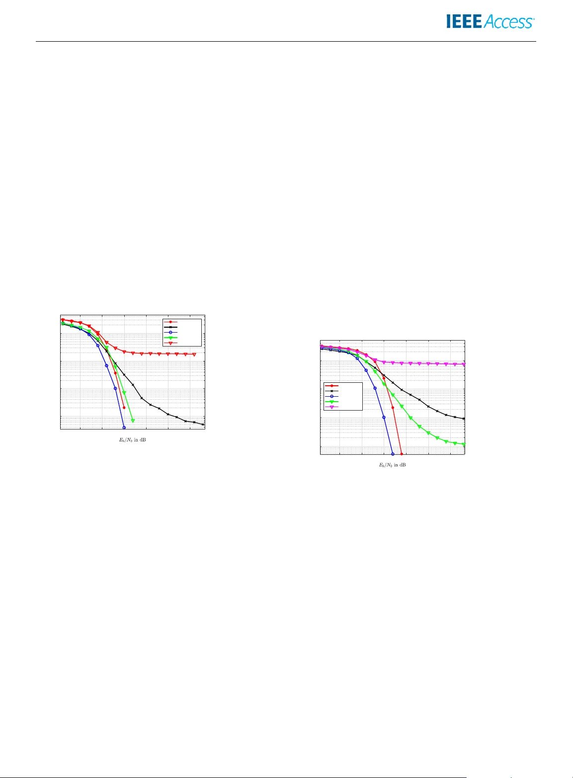
Date of publication xxxx 00, 0000, date of current v ersion xxxx 00, 0000. Digital Object Identiﬁer 11.1109/ACCESS.2021.DOI Lo w-Comple xity Decoder f or Overloaded Uniquel y Decodable Sync hr onous CDMA MICHEL KULHANDJIAN 1 , Senior Member , IEEE , HO V ANNES KULHANDJIAN 2 , Senior Member , IEEE , CLA UDE D’AMOURS 1 , Member , IEEE , HALIM Y ANIKOMER OGLU 3 , F ellow , IEEE , DIMITRIS A. P ADOS 4 , Senior Member , IEEE and GURGEN KHA CHA TRIAN 5 , Member , IEEE 1 School of Electrical Engineering and Computer Science, Univ ersity of Ottawa, Ottaw a, Ontario, K1N 6N5, Canada (e-mail: mkk6@buf falo.edu,cdamours@uottawa.ca) 2 Department of Electrical and Computer Engineering, California State Univ ersity , Fresno, Fresno, CA 93740, U.S.A. (e-mail: hkulhandjian@csufresno.edu) 3 Department of Systems & Computer Engineering, Carleton Univ ersity , Ottawa, Canada (e-mail: halim@sce.carleton.ca) 4 Computer & Electrical Engineering & Computer Science & I-SENSE Center , Florida Atlantic University , U.S.A., (e-mail: dpados@fau.edu) 5 College of Science & Engineering, American Uni versity of Armenia, Armenia, (e-mail: gurgenkh@aua.am) Corresponding author: Michel Kulhandjian (e-mail: mkk6@b uffalo.edu). ABSTRA CT W e consider the problem of designing a low-complexity decoder for antipodal uniquely decodable (UD) /errorless code sets for ov erloaded synchronous code-di vision multiple access (CDMA) systems, where the number of signals K a max is the largest known for the giv en code length L . In our complexity analysis, we illustrate that compared to maximum-likelihood (ML) decoder, which has an exponential computational complexity for e ven moderate code lengths, the proposed decoder has a quasi- quadratic computational complexity . Simulation results in terms of bit-error -rate (BER) demonstrate that the performance of the proposed decoder has only a 1 − 2 dB degradation in signal-to-noise ratio (SNR) at a BER of 10 − 3 when compared to ML. Moreov er , we deriv e the proof of the minimum Manhattan distance of such UD codes and we provide the proofs for the propositions; these proofs constitute the foundation of the formal proof for the maximum number users K a max for L = 8 . INDEX TERMS Uniquely decodable (UD) codes, overloaded CDMA, overloaded binary and ternary spreading spreading codes. NOMENCLA TURE 5G The ﬁfth generation 6G The sixth generation A WGN Additiv e white Gaussian noise BER Bit-error-rate BPSK Binary phase-shift ke ying CDM Code-division multiplexing CDMA Code-division multiple access eMBB Enhanced mobile broadband FD A F ast detection algorithm FDMA Frequency division multiple access LDS Low-density spreading MAI Multiple-access interference MF Matched ﬁlter MIMO Multiple-input multiple-output ML Maximum-likelihood MMSE Minimum mean-square estimation mMTC Massiv e machine-type-communications mmW av e Millimeter-w av e MO Multiple-orthogonal ND A Noiseless detection algorithm NOMA Non-orthogonal multiple access OMA Orthogonal multiple access PD A Probabilistic data association PIC Parallel interference cancellation PN Pseudo-noise SCMA Sparse code multiple access SIC Successiv e interference cancellation SNR Signal-to-noise ratio TDMA T ime-di vision multiple access UD Uniquely decodable uRLLC Ultra-reliable lo w-latency communications ZF Zero-forcing VOLUME 5, 2016 1 I. INTRODUCTION I N the last decade, wireless communication services hav e experienced explosiv e gro wth while communication tech- nologies hav e progressed generation by generation. In the previous generations spanning from 1G to 4G, the multiple access schemes were mostly characterized by orthogonal multiple access (OMA) techniques, where users are as- signed orthogonal resources in either frequency , (frequenc y- division multiple access (FDMA)), time, (time-division multiple access (TDMA)) or code, (code-division multiple access (CDMA)). CDMA [1] was the basic technology for 3G and for some 2G (IS-95) networks. High spectral- and power -ef ﬁciency , massive connectivity and low latency are among the requirements for next generation communica- tions and these requirements are expected to increase in the future, as researchers turn their ef forts to wards sixth generation (6G) wireless communications. Enhanced mobile broadband (eMBB), ultra-reliable low-latenc y communica- tions (uRLLC) and massi ve machine-type communication (mMTC) support a suite of compelling applications dri v- ing these requirements. Massiv e multiple-input multiple- output (MIMO), non-orthogonal multiple access (NOMA) and millimeter-wa ve (mmW ave) communications constitute promising techniques of addressing these stringent require- ments [2]. Supporting a large number of users communicating over a common channel may not be readily achiev able by OMA techniques due to the multiple-access interference (MAI) in rank-deﬁcient systems, where the number of users is greater than that of the resource blocks. T o meet the demand of increased bandwidth efﬁcienc y in synchronous CDMA, a CDMA concept was introduced in [3], which can support many more users for a gi ven code length compared to traditional CDMA. A number of signature design schemes have been studied for dense spreading in con ventional CDMA, where lo w cross-correlation sequence sets are designed to minimize the ov erall MAI, which allo ws more users to simultaneously access the common channel. This in turn results in increased spectral efﬁciency . Finding suitable spreading codes and decoding schemes for such ov erloaded systems is a challenging optimization problem. T o address these challenges, numerous non-uniquely de- codable (non-UD) [3]–[10], and UD [11]–[35] construction based code sets hav e been proposed. Examples of such non- UD code sets are pseudo-noise spreading (PN) [4], [5], or- thogonal/orthogonal CDMA (O/O), [6], [7], PN/orthogonal CDMA (PN/O) [3], multiple-orthogonal CDMA (MO) [8], improv ed O/O CDMA [9]. Those codes employ two or more sets of orthogonal signal wa veforms, which allows the system to accommodate more users than the signature length L . As a consequence of this, a signiﬁcant lev el of MAI exists at the output of each user’ s matched ﬁlter due to the non-zero cross-correlation of different signatures. Low cross-correlation sequence sets might not be the best criterion for very high rank-deﬁcient systems. One important criterion in such rank-deﬁcient systems is for the code set to be UD. By deﬁnition the UD codes are those in which the data of different users can be unambiguously decoded in a noiseless channel using linear recursive decoders [31]. Low- complexity linear decoders were introduced for these UD code sets using either binary { 0, 1 } , or antipodal {± 1 } , or alternativ ely ternary { 0, ± 1 } chips in [27]–[30], [32]–[35]. On the other hand, Lu et al. [36] proposed M -ary code sets for the multiple-access adder channel. V arious applications hav e been implementing UD code sets framew ork such as in multi-way physical-layer network coding conceiv ed in [33], [37]. All of these multiple access concepts were introduced in order to serve a number of excess users beyond the av ailable resources. These multiple access schemes are characterized by NOMA techniques [38] in 5G and beyond wireless com- munications. Recently , sev eral NOMA solutions have been activ ely in vestigated [2], which can be basically di vided into two main categories, namely power -domain and code- domain NOMA. A few of the strong contenders of code- domain NOMA are low-density spreading aided CDMA (LDS-CDMA) [39], [40] and sparse code multiple access (SCMA) [41], [42]. LDS-CDMA [39], [40] must generally guarantee to be UD code set [43], which means non- zero Euclidean distance. The design of LDS type matrices offers ﬂexible resource allocation, performs better in terms of handling the MAI that exists in rank-deﬁcient systems and has low-comple xity recei vers compared to con ventional CDMA. Unlike the dense UD code set, the LDS-CDMA structure can be represented by a factor graph, the classic message passing algorithm (MP A) can be emplo yed for its detec- tion. Due to the reason that UD code sets were originally designed for adder channels, generally a simple noiseless detection is de veloped. Howe ver in practice, the wireless transmission channel exhibits, among other things, selecti ve fading, multipath and the near-far problem, which leads to unequal receiv ed po wer among users. Consequently , if syn- chronization, channel equalization are compensated, low- complexity detectors can be applied to wireless channels. Inspired by these attracti ve features of UD code sets, this paper in vestigates UD codes for synchronous uplink NOMA. In the case of dispersiv e fading channels, we can potentially equalize the channel effect by using chan- nel precoding. Therefore, we consider de veloping a low- complexity detector for UD code sets that are proposed in [31] for ov erloaded synchronous CDMA systems. It is widely recognized that the comple xity of an optimal detector is exponentially proportional to the number of users, which prohibits its practical implementation. V arious suboptimal low-comple xity detection techniques have been already pro- posed. These suboptimal approaches can be classiﬁed into two categories: linear and non-linear multiuser detectors. Linear multiuser detectors include among others, matched ﬁlter (MF), minimum mean-square error (MMSE), and zero- forcing (ZF), etc. In a non-linear subtracti ve interference cancellation detector the interference is ﬁrst estimated and 2 V OLUME 5, 2016 then it is subtracted from the recei ved signal before de- tection. The cancellation process can be carried out either successiv ely (SIC) [44], or in parallel (PIC) [45]–[47]. In non-linear iterativ e detectors [48]–[52], probabilistic data association (PDA) [53] aims to suppress the MAI in each iteration in order to improv e the ov erall error performance. Suboptimal polynomial time detectors that are based on the geometric approach are studied in [54], [55]. In general, linear as well as non-linear detectors cannot separate users in ov erloaded systems e ven in the case of asymptotically vanishing noise. Therefore, the spreading codes must ha ve property such that decoding can achie ve asymptotically zero probability of error multiuser detec- tion when the signal-to-noise (SNR) ratio becomes arbi- trary large. The UD class of codes that guarantee “error- less” communication in an ideal (noiseless) synchronous CDMA/code-division multiplexing (CDM) also shows a good performance in the presence of noise. Finding the overloaded UD class of codes for noiseless channel is directly related to coin-weighing problem, one of the problems that is discussed by Erd ˝ os and Rén yi in [11]. It can be considered as a special case of a general problem where authors in [12], [13], [16], [25], [26] refer to them as detecting matrices. Lindström in [15] deﬁnes the same problem as the detecting set of v ectors. Giv en an integer q ≥ 2 and a ﬁnite set alphabet M of rational integers, let v k for 1 ≤ k ≤ K be L -dimensional (column) vectors with all components from M such that the q K sums K X k =1 v k  k (  k = 0, 1, 2, . . . , q − 1) (1) are all distinctly unique, then { v 1 , . . . , v K } are detecting set of vectors. Let F q ( L ) be the maximal number of L - dimensional vectors and f q ( K ) be the minimal vector length to form a detecting matrix for a gi ven length L and a number of v ectors K . The problem of determining f q ( K ) as a special case when q = 2 , M = { 0, 1 } that can be equi valently expressed as a coin-weighing problem: what is the minimal number of weighings on an accurate scale to determine all false coins in a set of K coins. The choice of coins for a weighing must not depend on results of previous weighings. This problem was ﬁrst introduced by Söderberg and Shapiro [12] for K = 5 . The minimal number of weighings, L , has only been found for a fe w different values of K in [17]. Howe ver , Lindström gives an explicit construction of L × γ ( L + 1) binary (alphabet { 0, 1 } ) and L × γ ( L ) + 1 antipodal (alphabet {± 1 } ) detecting matrices [14], where γ ( L ) i is the number of ones in the binary expansion of all positiv e integers less than L . He also proved that the lower bound in the case of M = { 0, 1 } or {± 1 } is lim K →∞ f 2 ( K ) log K K = 2. (2) i As an example, γ (8) = 12 . Cantor and Mills [16] constructed a class of 2 i × ( i +2)2 ( i − 1) ternary (alphabet { 0, ± 1 } ) detecting matrices for i ∈ Z + , which implies that in the case of M = { 0, ± 1 } the lower bound is lim K →∞ f 3 ( K ) log K K ≤ 2. (3) In the literature, most of the explicit construction of UD code sets are recursi ve [18]–[35]. T o the best of our kno wl- edge, it is worth mentioning that the maximum number of vectors of the explicit constructions of binary , antipodal and ternary code sets are K b max = γ ( L + 1) , K a max = γ ( L ) + 1 and K t max = ( i + 2)2 ( i − 1) , as sho wn in T able 1, T able 2 and T able 3, respectiv ely . Sev eral authors have proposed decoders with linear complexity in noiseless scenarios for the explicit construction, where the detecting matrix has the known-to-us maximum number of vectors, K max . For noisy channels, recently in [28], a class of antipodal code sequences, for ov erloaded CDM systems with sim- pliﬁed two-stage maximum-likelihood (ML) detection, has been proposed. In addition to that, other ov erloaded matrices ov er the ternary alphabet are introduced in [29] with a lo w- complexity decoding algorithm. Similarly , in [30] the au- thors propose ov erloaded code sets over the ternary alphabet that has a twin tree structured cross-correlation hierarchy that can be decoded with a simple multi-stage detector . Y et another construction of ternary codes that increases the number of columns, K , of UD codes for a such length compared to those proposed in [29] and [30] with a low- complexity polynomial time decoder is proposed in [32]. The primary reason for such lo w-complexity decoders is that the code sets are constructed with a certain criteria, which entails lowering the maximum number of users K < K max , as sho wn in T able 3. Apart from, binary , antipodal and ternary UD spreading codes higher alphabet k -ary spreading codes were studied by Lu et al. [56] for the multiple-access adder channels. In this work, for the ﬁrst time we consider the problem of designing a low-comple xity decoder that has a complexity of O ( LK log 2 ( K )) for UD code sets in [31] ha ving the maximum number of users K a max . The code sets presented in [31] are also recursi ve, which make use of a linear map between vector spaces to Galois ﬁeld extensions. These UD code sets are one possible construction of all possible dis- tinct UD code sets, sho wn in T able 2. Simulation results in terms of bit-error-rate (BER) demonstrate that the proposed decoder has a degradation of only 1 − 2 dB in SNR compared to the ML decoder at a BER of 10 − 3 . Our contrib utions are summarized as follows: (1) W e present the proofs for the important Propositions 1-4 that are presented for the ﬁrst time in [31]. Those new prepositions are actually the broken down versions of the unique decodability (UD) property . (2) Moreov er , for the ﬁrst time, based on Propositions 1-4 , we formally prov e that the maximum number of users for the gi ven L = 8 is K a max = 13 . VOLUME 5, 2016 3 T ABLE 1. Binar y Codes Y ear A uthors and Publications Rows Columns Decoder Noiseless A WGN 1963 Söderberg and Shapiro [12] L < γ ( L + 1) No No 1964 Lindström [14] L γ ( L + 1) † No No 1966 Cantor and Mills [16] 2 i − 1 i 2 ( i − 1) No No 1989 Martirossian and Khachatrian [22] L γ ( L + 1) Y es No 2019 Kulhandjian et al. [34] L γ ( L + 1) Y es Y es † Code set constructions that achie ve the maximum number of vectors K max are presented in bold. T ABLE 2. Antipodal Codes Y ear A uthors and Publications Rows Columns Decoder Noiseless A WGN 1964 Lindström [14] L γ ( L ) + 1 No No 1987 Khachatrian and Martirossian [21] L γ ( L ) + 1 No No 1995 Khachatrian and Martirossian [23] 2 i i 2 ( i − 1) + 1 Y es No 2012 Kulhandjian and Pados [31] 2 i i 2 ( i − 1) + 1 Y es No T ABLE 3. T er nary Codes Y ear A uthors and Publications Rows Columns Decoder Noiseless A WGN 1966 Cantor and Mills [16] 2 i ( i + 2)2 ( i − 1) No No 1979 Chang and W eldon [18] 2 i ( i + 2)2 ( i − 1) Y es No 1982 Ferguson [19] 2 i ( i + 2)2 ( i − 1) Y es No 1984 Chang [20] 2 i ( i + 2)2 ( i − 1) No No 1998 Khachatrian and Martirossian [24] 2 i ( i + 2)2 ( i − 1) Y es No 2012 Mashayekhi and Marvasti [29] 2 i 2 ( i +1) − 1 Y es Y es 2016 Singh et al. [30] 2 i 2 ( i +1) − 2 Y es Y es 2018 Kulhandjian et al. [32] 2 i 2 ( i +1) + 2 ( i − 2) − 1 Y es Y es 2021 Kulhandjian et al. [35] 2 i i 2 ( i − 1) + 1 Y es Y es (3) The minimum Manhattan distance is proved to be 4 for the recursi ve UD code sets in [31]. (4) W e develop a low-comple xity decoder that has a com- plexity of O ( LK log 2 ( K )) for our dev eloped UD code sets in [31] having the maximum number of users K a max . (5) W e compute the complexity of the deterministic noise- less detection algorithm (ND A) presented in [31] and perform some complexity analysis for the proposed f ast (low-comple xity) detection algorithm (FD A). The rest of the paper is organized as follo ws. The mini- mum Manhattan distance of code sets in [31] is presented in Section IV, followed by the proofs of the Propositions 1-4 and the maximum number of K a max for the case of L = 8 in Sections II and III, respectiv ely . Detailed discussion of the FD A is presented in Section V. The complexity analysis for both ND A and FD A algorithms is presented in Section VI. After illustrating simulation results in Section VII, a few conclusions are dra wn in Section VIII. The following notations are used in this paper . All boldface lower case letters indicate column vectors and upper case letters indicate matrices, () T denotes transpose operation, mo d denotes the modulo operation, sgn denotes the sign function, and | · | denotes cardinality of the set. II. PROOF OF PR OPOSITIONS In order to f acilitate the de velopment of the proof it is beneﬁcial to present the UD code set in [31] which are constructed as C = [ H L V L ] ∈ {± 1 } L × K , where V L ∈ {± 1 } L × ( K − L ) . W e recall that the Sylvester - Hadamard matrix of order 2 is H 2 = h 1 1 1 − 1 i and of order 2 p +1 for p = 1, 2, ... is H 2 p +1 = h H 2 p H 2 p H 2 p − H 2 p i . Then, for any p = 1, 2, ... , H 2 p H 2 p = 2 p I 2 p × 2 p , where I N × N is the N × N identity matrix. W e introduce the notation H 4 = [ h 0 , h 1 , h 2 , h 3 ] , [ a 0 , a 1 , a 2 , a 3 ] , h [ − 1, 1, 1, 1] T , [1, − 1, 1, 1] T , [1, 1, − 1, 1] T , [1, 1, 1, − 1] T i , and the negation function x − , − x . W e can see that set of vectors G = { h 0 , h 1 , h 2 , h 3 , a 0 , a 1 , a 2 , a 3 } together with  4 V OLUME 5, 2016 operator form a ﬁnite group ( G ,  ) . There exists an isomor- phism ϕ , shown in T able 4 from G to ﬁnite additiv e Abelian group ( F 2 4 , +) of extended Galois ﬁeld F 2 4 , in other words G is isomorphic to ( F 2 4 , +) , ( G ,  ) ∼ = ( F 2 4 , +) . From linear algebra we know that there is an isomorphism from ﬁnite additi ve groups ( F p n , +) to v ector ﬁelds ( F n p , +) and to Z n p , that is ( F p n , +) ∼ = ( F n p , +) ∼ = Z n p , [57]. T able 4 shows the mapping of the v ectors h 0 , ..., h 3 , a 0 , .., a 3 and its negated forms to elements in F 2 4 with primitiv e polynomial α 4 + α + 1 = 0 , where α is the primiti ve element in extended Galois ﬁeld GF (2 4 ) . Notice carefully that operation of the ﬁnite group G is  , whereas the ﬁnite additiv e group F 2 4 is + . T ABLE 4. Isomor phism ϕ : G 7→ F 2 4 Antipodal Polynomial Power h 0 0 0 h 2 1 1 h 1 α α h − 0 α 2 α 2 a 1 α 3 α 3 h 3 α + 1 α 4 h − 1 α 2 + α α 5 a − 1 α 3 + α 2 α 6 a 2 α 3 + α + 1 α 7 h − 2 α 2 + 1 α 8 a 3 α 3 + α α 9 h − 3 α 2 + α + 1 α 10 a − 3 α 3 + α 2 + α α 11 a − 2 α 3 + α 2 + α + 1 α 12 a 0 α 3 + α 2 + 1 α 13 a − 0 α 3 + 1 α 14 W ith the abo ve formulation, the columns of V L , F ϕ : {± 1 } L × 1 7→ F L 0 × 1 2 4 , f i = F ϕ ( v i ) maps the i -th column v i to f i , for i = 0, ..., K − L − 1 , where f i = [ f i ,0 f i ,1 , . . . , f i , L 0 ] T , f i , j ∈ { 0, 1, α , ..., α 14 } , 0 ≥ j ≥ L 0 , L 0 = L/ 4 = 2 p − 2 for p ≥ 2 . As an example for V 8 the mapped vectors are as two-dimensional v ectors f i = [ f i ,0 f i ,1 ] T . In order to prove Proposition 1-4 that was ﬁrst presented in [31], we will expose some very interesting claims. One property of the Hadamard matrix is the following, if we replace 1 ’ s in Hadamard matrix with 0 ’ s, and replace the − 1 ’ s with 1 ’ s we create L − 1 Hadamard binary channel codes, since the ﬁrst column results in zero vector [58]. Let the Hadamard columns H L = [ h 0 , ..., h L − 1 ] be mapped into linear binary codes B L = [ b 0 , ..., b L − 1 ] . There is an isomorphism between binary addition and multiplication of {± 1 } elements. Consequently , since binary addition of Hadamard linear codes is a Hadamard code itself then it is equiv alent to element-wise multiplication of an y Hadamard codes H L is also in H L . Therefore, some properties can be deriv ed. W e denote the mapping of h i for i = 0, ..., L − 1 vectors into binary b i ∈ { 0, 1 } L × 1 vectors by b i = f ( h i ) and in verse h i = f − 1 ( b i ) , where H L = [ h 0 , ..., h L − 1 ] and B L = [ b 0 , ..., b L − 1 ] . Deﬁne the f ( x ) = ( 1 − x ) / 2 and the inv erse f − 1 ( y ) = [( − 1) y 0 , ..., ( − 1) y L − 1 ] functions. Then, the j th column corresponds to linear combination of b j = j 1 b 1 ⊕ j 2 b 2 ⊕ j 4 b 4 ⊕ ... ⊕ j 2 p b 2 p , where j has the binary representation j = j 1 + 2 j 2 + 4 j 4 + ... + 2 p j 2 p [58]. Here ⊕ is modular 2 summation and j l ∈ { 0, 1 } for l = { 1, 2, 4, ..., 2 p } . Therefore, the resulting code is linear code b k =  0 b 0 ⊕  1 b 1 ⊕ ... ⊕  L − 1 b L − 1 for all  i ∈ { 0, 1 } , where b k ∈ B L . T ABLE 5. Binar y addition and {± 1 } multiplication Binary Bipolor 0 + 0 = 0 1 × 1 = 1 0 + 1 = 1 1 × -1 = -1 1 + 0 = 1 -1 × 1 = -1 1 + 1 = 0 -1 × -1 = 1 Let us look at the problem and assume that Null ( C ) ∈ Z , where Z ∈ { 0, ± 1 } K × 1 excluding trivial case { 0 } K × 1 and let z ∈ Z . Then the nullspace of C can be formulated as such Cz = 0 (4a) [ H L V ] z = 0 L (4b) H L z 1 + V L z 2 = 0 (4c) H L z 1 = − V L z 2 . (4d) where z =  z T 1 z T 2  T , z 1 ∈ { 0, ± 1 } L × 1 , z 2 ∈ { 0, ± 1 } ( K − L ) × 1 and 0 = { 0 } L × 1 . If we assume z 1 = 0 and for some z 2 (4) is true, then (4) can be expressed in terms of V L only as V L z 2 = 0 . (5) Claim 1. Element-wise multiplication of H L ’ s columns h j =  0 h 0   1 h 1  ...   L − 1 h L − 1 for all possible 0 ≤ i ≤ L − 1 ,  i ∈ { 0, 1 } is true, where h j ∈ H L . Claim 2. If V L does not intersect 0 over the non-trivial { 0, ± 1 } combinations and (4) is true, then β 0 v 0  β 1 v 1  ...  β K − L − 1 v K − L − 1 = α h j must be true for some β i ∈ { 0, 1 } , 0 ≤ i ≤ K − L − 1 , α ∈ {± 1 } . However , if β 0 v 0  β 1 v 1  ...  β K − L − 1 v K − L − 1 = α h j for some β i ∈ { 0, 1 } , 0 ≤ i ≤ K − L − 1 , α ∈ {± 1 } is true then it is not necessary that (4) is also true. Claim 3. If (5) is true, then β 0 v 0  β 1 v 1  ...  β K − L − 1 v K − L − 1 = ± 1 must be true for some β i ∈ { 0, 1 } , 0 ≤ i ≤ K − L − 1 and 1 which is all one vector of dimension L × 1 . Howe ver , if β 0 v 0  β 1 v 1  ...  β K − L − 1 v K − L − 1 = ± 1 for some β i ∈ { 0, 1 } , 0 ≤ i ≤ K − L − 1 is true then it is not necessary that (5) is also true . Claim 4. If V L does not satisfy (4) and (5) then multiplying any column of V L by − 1 will still not satisfy (4) and (5). Authors in [31] sho wed by exhausti ve search that in case when L = 4 then K a max = 5 and all the possible candidates are [ − 1, 1, 1, 1] T , [1, − 1, 1, 1] T , [1, 1, − 1, 1] T , [1, 1, 1, − 1] T and their negati ves according to the Claim 4. Furthermore, we continue to present additional claims. Let v i ∈ {± 1 } 4 for 0 ≤ i ≤ N − 1 then, VOLUME 5, 2016 5 Claim 5. If β 0 v 0  β 1 v 1  ...  β N − 1 v N − 1 = α h j and α ∈ {± 1 } , h j ∈ H 4 then ∀ N ∈ N , [ v 0 , ..., v N − 1 ] A v 1 = H 4 A H 1 is true for some β i ∈ { 0, 1 } , 0 ≤ i ≤ N − 1 , N 0 ∈ N is not necessarily equal to N , A v ∈ { 0, ± 1 } N × N , A H ∈ { 0, ± 1 } 4 × N 0 , which have maximum one ± 1 entry in each column and 0 ’ s elsewher e. Claim 6. If 0 = N mod 2 and β 0 v 0  β 1 v 1  ...  β N − 1 v N − 1 = ± 1 then [ v 0 , ..., v N − 1 ] A v 1 = 0 is true for some β i ∈ { 0, 1 } , 0 ≤ i ≤ N − 1 , A v ∈ { 0, ± 1 } N × N , which have maximum one ± 1 entry in eac h column and 0 ’ s elsewher e, e xcept when N = 4 and v 0 = [ − 1, 1, 1, 1] T , v 1 = [1, − 1, 1, 1] T , v 2 = [1, 1, − 1, 1] T , v 3 = [1, 1, 1, − 1] T . The generalization of Claims 1-6 formalizes the Propo- sitions 1-4 and hence we presented the proofs. III. PROOF K A MAX = 13 FOR L = 8 For the case when L = 8 , we prove that the maximum number of columns we can append to H 8 is actually K a max − L = 5 . Note that all proposed UD or another words one- to-one matrix constructions in literature are C ⊂ C , where C is all possible antipodal UD code sets for a giv en L . In order to prov e for the maximum number of possible vectors K a max , we should look at all possible V and count how many structure of V hits any of the forbidden lattice points H m z 1 and how many does not. If for a gi ven k column, we count the number of V that hits any forbidden lattice points is equal to the total number of possible V vector set, then we kno w that maximum number of columns of V that does not hit any forbidden lattice points should be smaller than k . First, we transform antipodal vectors into polynomials with integer coef ﬁcients Z [ x ] , F : {± 1 } m × 1 7→ Z [ x ] . Those polynomials represent the ro w location and number of − 1 s or +1 s in any antipodal v ∈ {± 1 } m × 1 with dimension m . Let the polynomial be G ( x ) = a 0 x 0 + a 1 x 1 + a 2 x 2 + ... + a m − 1 x m − 1 , (6) where a i ∈ Z . Additions of vector v in vector space is equiv alent to the addition of Z [ x ] in polynomial space. Each antipodal vectors, v j ∈ {± 1 } m × 1 , where 0 ≤ j ≤ 2 m − 1 , is mapped to the corresponding polynomials G j n ( x ) and G j p ( x ) to represent the +1 and − 1 of the v j . As an example, for m = 4 , the antipodal vector , v 10 = [1, − 1, 1, − 1] T , is mapped to G 10 n ( x ) = x 1 + x 3 and G 10 p ( x ) = x 0 + x 2 polyno- mials. Observe that for any antipodal vector v j , the addition of polynomials, G j n ( x ) + G j p ( x ) = x 0 + x 1 + ... + x m − 1 . In order to visualize polynomial additions in 2 -dimensional Euclidean space we can further transform Z [ x ] vector space into Λ ⊆ Z 2 integer lattice, H : Z [ x ] 7→ Z 2 . Let us deﬁne functions σ j n ( m ) = G j n ( m ) , σ j p ( m ) = G j p ( m ) , which are the evaluations of polynomials G j n ( x ) and G j p ( x ) at m , where m is the dimension of vector v j . By setting the x-axis and y-axis to be G j n ( x ) and G j p ( x ) , we can build Λ ⊆ Z 2 lattice points, since e valuations σ j n ( m ) and σ j p ( m ) for each antipodal v j vectors are integers. T aking the above example of antipodal vectors having dimension of m = 4 the equi valent integer lattice points is sho wn in T able 6. FIGURE 1. Addition of lattice points in Λ ⊆ Z 2 , m = 4 . Let us deﬁne sublattices Λ H ⊆ Λ and Λ V 0 ⊆ Λ constructed by v ectors of [ H 4 − H 4 ] and V 0 , where V 0 ∈ {± 1 } 4 × 8 , v 0 i / ∈ [ H 4 − H 4 ] for 1 ≤ i ≤ 8 . As a reminder , for the antipodal UD code set the goal is to construct V 0 with the maximum number of columns K a max − L such that Λ H ∩ Λ V 0 = ∅ . Fig. 1 demonstrates a hit, in other words Λ H ∩ Λ V 0 6 = ∅ for k = 2 and V 0 = [ v 4 , v 14 ] = h [1, 1, − 1, 1] T [1, − 1, − 1, − 1] T i , which is equiv alent to [16, 69] T and [84, 1] T in Λ V 0 . If we construct the third and the fourth columns to be v 6 = [1, − 1, − 1, 1] T and v 12 = [1, 1, − 1, − 1] T , equiv alently [20, 65] T and [80, 5] T in Λ H of H 4 adding them we get [2, 0, − 2, 0] T , which is sho wn as a lattice point [100, 70] T in Fig. 1. Clearly , addition of [16, 69] T and [84, 1] T lattice points also results [100, 70] T , hence, this is why intersection of two sublattices is not an empty set. Therefore, it can be sho wn that all possible  8 2  combination of two columns of V 0 will at least hit a lattice points of Λ H , which means that Λ H ∩ Λ V 0 6 = ∅ for k = 2. Hence, | V 0 | = 1 for the case of m = 4 . Using this approach, we can construct sublattices Λ H and Λ V 0 for the case of m = 8 and ﬁnd the upper bound of k such that Λ H ∩ Λ V 0 = ∅ . This creates a framework to search the solution using geometric combinatorics (e.g. Minko wski sum, Minko wski geometry of numbers [59]), partition and decomposition of Λ into equiv alence classes, formed by sublattices and its’ cosets to prov e the K a max we can have for a gi ven m and ho w to generate those v ectors in V 0 . 6 V OLUME 5, 2016 T ABLE 6. Lattice points for all antipodal vectors v when m = 4 j 0 1 2 3 4 5 6 7 8 9 10 11 12 13 14 15 G j n ( m ) 0 1 4 5 16 17 20 21 64 65 68 69 80 81 84 85 G j p ( m ) 85 84 81 80 69 68 65 64 21 20 17 16 5 4 1 0 Polynomials of G j n ( x ) and G j p ( x ) can also be represented by their exponents in the above e xample G 10 n ( x ) → E 10 n = { 1, 3 } and G 10 p ( x ) → E 10 p = { 0, 2 } . Therefore, our problem of av oiding non-tri vial combinations of V to hit any forbidden lattice points becomes ] h t ∈ H m E t i 6 = ] v t ∈ V E t j i , j ∈ { p , n } , (7) where U denotes the multiset union, element-wise sums of each multisets and 1 ≥ t ≥ 2 m − 1 integer v alue corresponds to antipodal v ector . The objecti ve is to a void V U v t ∈ V E t j sums of multisets E p or E n of V to hit any forbidden U h t ∈ H m E t i sum of multisets E p or E n of H m . Obviously , there are 3 m forbidden multisets of H m and we do not want 3 k − 1 multisets of V excluding tri vial case hit any of the forbidden multisets. W e can use multiset partition theories and study bipolar vectors by their E p and E n representations and prov e the maximal number of k . Note that in our matrix construction design of the v i ’ s that they are distinct and not equal to any of columns of H m or − H m . If, ho wever , any of v i ∈ ± H m , then the multiset of v i hits the forbidden multiset of H m . Such v i vectors can nev er be included in vector set of UD codes. Additionally , the v i s can be replaced by − v without violating the uniquly decodability property (4). Since all possible combinations of vectors including − v of V do not hit any of the forbidden multisets. In other words, if [ H m V ] ∈ C so is any number of columns of V or H m multiplied by − 1 . One way to approach this problem is to classify all v bipolar vectors into groups then use inclusion-e xclusion principle. There are 2 m number of v ’ s that consist of | E n | = i , where i = { 0, 1, ..., m } with all the combinations makes P m i =0  m i  = 2 m . Let us divide the total number of m -dimensional bipolar vectors into two classes; v ∈ B + m if 0 ≤ | E n | < m/ 2 , | E n | = m/ 2 | E p = { 1, 2, .. } excluding m h i ’ s columns from H m and v ∈ B − m if m/ 2 < | E n | ≤ m , | E n | = m/ 2 | E n = { 1, 2, .. } excluding m − h i ’ s columns from − H m . It’ s clear that if any v ∈ B + m then − v ∈ B − m . This narrows for our design to consider only distinct vector sets and the total number of such distinct v i ’ s to be considered in our V design is P m/ 2 i =0  m i  − m = 2 m − 1 − m . W e need to construct from distinct vectors v ∈ B + m such that they do not hit any forbidden multisets. Therefore, the total possible number of V sets with k columns is  2 m − 1 − m k  . Out of this total number of V sets with k columns only some satisfy UD or one-to-one condition when appended to H m . If all the possible V ’ s do not satisfy one-to-one condition that means k exceeds the maximum number of columns that can be added to H m . Hence, we want to count how many combinations of v ∈ B + m with k columns hit the forbidden multisets. If the number of combination is equal the total number of V sets then we know that k is not the maximum. Counting that number will help us to prove the maximum number of columns k . W e classify B + m into different groups, so that any com- binations of vectors in similar group hits the forbidden multisets and therefore, such v that belong to the same group must be avoided in our design. In our example, for m = 8 and k = 2 , we classify B + 8 into groups and count how many V ’ s do not satisfy the UD condition or one-to-one condition out of  2 8 − 1 − 8 2  =  120 2  = 7140 possible vector sets. By looking at all possible combinations of V = [ v j 1 v j 2 ] , | E j 1 n | , | E j 2 n | ∈ { 1, ..., 8 } we only consider ( | E j 1 n | , | E j 2 n | ) = { (1, 3), (2, 2), (3, 3), (4, 4) } . Since to hit [ h 1 ± h i ] , where 2 ≤ i ≤ 8 , the vectors [ v j 1 v j 2 ] must hav e ( | E j 1 n | , | E j 2 n | ) = (1, 3) and ( | E j 1 n | , | E j 2 n | ) = (2, 2) . W e can easily sho w that if [ v j 1 v j 2 ] hit forbidden multisets with ( | E j 1 n | , | E j 2 n | ) = (1, 3) and ( | E j 1 n | , | E j 2 n | ) = (2, 2) then [ − v j 1 − v j 2 ] with ( | E j 1 n | , | E j 2 n | ) = (7, 5) and ( | E j 1 n | , | E j 2 n | ) = (6, 6) hit [ − h 1 ∓ h l ] and l 6 = i . Also, if [ v j 1 v j 2 ] hit forbidden multisets with ( | E j 1 n | , | E j 2 n | ) = (2, 2) then [ − v j 1 v j 2 ] and [ v j 1 − v j 2 ] with ( | E j 1 n | , | E j 2 n | ) = (2, 6) hit [ ± h l ± h p ] and i 6 = l , p 6 = i . Hitting [ ± h i ± h j ] , where 2 ≤ i 6 = j ≤ 8 multisets then v ectors must ha ve ( | E j 1 n | , | E j 2 n | ) = (3, 5) and ( | E j 1 n | , | E j 2 n | ) = (4, 4) . Since we only work with distinct vectors B + 8 then ( | E j 1 n | , | E j 2 n | ) = (3, 5) that has [ v j 1 − v j 2 ] is equiv alent to [ v j 1 v j 2 ] with ( | E j 1 n | , | E j 2 n | ) = (3, 3) . Now , let us classify ( | E j 1 n | , | E j 2 n | ) = (1, 3) , ( | E j 1 n | , | E j 2 n | ) = (2, 2) , ( | E j 1 n | , | E j 2 n | ) = (3, 3) , ( | E j 1 n | , | E j 2 n | ) = (4, 4) into A i ’ s, D i ’ s, F i ’ s and G i ’ s groups. W e kno w that the total number of v s with | E n | = 1 is  8 1  = 8 , | E n | = 2 is  8 2  = 28 , | E n | = 3 is  8 3  = 56 and | E n | = 4 is  8 4  = 70 . Here is how we divide 56 of | E n | = 3 and 8 of | E n | = 1 into A i ’ s, 1 ≤ i ≤ 8 groups. A 1 =       − 1 1 1 1 1 1 1 1             1 1 1 1 1 1 1 − 1 − 1 − 1 1 1 1 1 − 1 1 1 − 1 − 1 1 1 − 1 1 1 1 1 − 1 − 1 1 − 1 1 − 1 1 − 1 1 1 − 1 1 1 − 1 1 − 1 1 1 − 1 − 1 1 1 − 1 1 1 − 1 1 − 1 − 1 1       , VOLUME 5, 2016 7 A 2 =       1 − 1 1 1 1 1 1 1             − 1 − 1 − 1 1 1 1 1 1 1 1 1 1 1 1 − 1 1 1 − 1 − 1 1 1 − 1 1 1 1 1 − 1 − 1 1 − 1 1 − 1 1 − 1 1 1 − 1 1 1 − 1 1 − 1 1 1 − 1 1 − 1 − 1 1 1 1 − 1 − 1 1 1 − 1       , A 3 =       1 1 − 1 1 1 1 1 1             − 1 − 1 − 1 1 1 1 1 − 1 1 1 − 1 − 1 1 1 1 1 1 1 1 1 1 − 1 1 1 1 1 − 1 − 1 1 − 1 1 − 1 1 − 1 1 1 1 − 1 1 − 1 − 1 1 1 − 1 1 1 − 1 1 − 1 1 1 − 1 − 1 1 1 − 1       , A 4 =       1 1 1 − 1 1 1 1 1             − 1 − 1 − 1 1 1 1 1 − 1 1 1 − 1 − 1 1 1 − 1 1 1 1 1 − 1 − 1 1 1 1 1 1 1 1 1 − 1 1 − 1 1 − 1 1 1 1 − 1 1 − 1 − 1 1 1 1 − 1 − 1 1 1 − 1 1 − 1 1 1 − 1 1 − 1       , A 5 =       1 1 1 1 − 1 1 1 1             − 1 − 1 − 1 1 1 1 1 − 1 1 1 − 1 − 1 1 1 1 − 1 1 − 1 1 − 1 1 1 1 − 1 1 − 1 − 1 1 1 1 1 1 1 1 1 − 1 1 1 1 1 − 1 − 1 1 − 1 1 1 − 1 1 − 1 1 1 − 1 − 1 1 1 − 1       , A 6 =       1 1 1 1 1 − 1 1 1             − 1 − 1 − 1 1 1 1 1 − 1 1 1 − 1 − 1 1 1 1 − 1 1 − 1 1 − 1 1 1 1 − 1 1 − 1 − 1 1 − 1 1 1 1 1 − 1 − 1 1 1 1 1 1 1 1 1 1 − 1 − 1 1 1 − 1 1 − 1 1 1 − 1 1 − 1       , A 7 =       1 1 1 1 1 1 − 1 1             − 1 − 1 − 1 1 1 1 1 − 1 1 1 − 1 − 1 1 1 1 − 1 1 − 1 1 − 1 1 1 1 − 1 1 − 1 − 1 1 1 − 1 1 1 − 1 1 − 1 1 1 − 1 − 1 1 1 − 1 1 1 1 1 1 1 1 − 1 1 1 1 1 − 1 − 1       , A 8 =       1 1 1 1 1 1 1 − 1             − 1 − 1 − 1 1 1 1 1 − 1 1 1 − 1 − 1 1 1 1 − 1 1 − 1 1 − 1 1 1 1 − 1 1 − 1 − 1 1 1 1 − 1 − 1 1 1 − 1 1 − 1 1 1 − 1 1 − 1 − 1 1 1 1 1 − 1 − 1 1 1 1 1 1 1 1       equiv alently , we can then write them in multiset form as A 1 = E p = { 1, 2, 3, 4, 5, 6, 7 } E n = { 0 } E p = { 0, 4, 5, 6, 7 } E n = { 1, 2, 3 } E p = { 0, 2, 3, 6, 7 } E n = { 1, 4, 5 } E p = { 0, 2, 3, 4, 5 } E n = { 1, 6, 7 } E p = { 0, 1, 3, 5, 7 } E n = { 2, 4, 6 } E p = { 0, 1, 3, 4, 6 } E n = { 2, 5, 7 } E p = { 0, 1, 2, 5, 6 } E n = { 3, 4, 7 } E p = { 0, 1, 2, 4, 7 } E n = { 3, 5, 6 } A 2 = E p = { 0, 2, 3, 4, 5, 6, 7 } E n = { 1 } E p = { 1, 4, 5, 6, 7 } E n = { 0, 2, 3 } E p = { 1, 2, 3, 6, 7 } E n = { 0, 4, 5 } E p = { 1, 2, 3, 4, 5 } E n = { 0, 6, 7 } E p = { 0, 1, 3, 5, 6 } E n = { 2, 4, 7 } E p = { 0, 1, 3, 4, 7 } E n = { 2, 5, 6 } E p = { 0, 1, 2, 5, 7 } E n = { 3, 4, 6 } E p = { 0, 1, 2, 4, 6 } E n = { 3, 5, 7 } A 3 = E p = { 0, 1, 3, 4, 5, 6, 7 } E n = { 2 } E p = { 2, 4, 5, 6, 7 } E n = { 0, 1, 3 } E p = { 1, 2, 3, 5, 7 } E n = { 0, 4, 6 } E p = { 1, 2, 3, 4, 6 } E n = { 0, 5, 7 } E p = { 0, 2, 3, 5, 6 } E n = { 1, 4, 7 } E p = { 0, 2, 3, 4, 7 } E n = { 1, 5, 6 } E p = { 0, 1, 2, 6, 7 } E n = { 3, 4, 5 } E p = { 0, 1, 2, 4, 5 } E n = { 3, 6, 7 } A 4 = E p = { 0, 1, 2, 4, 5, 6, 7 } E n = { 3 } E p = { 1, 4, 5, 6, 7 } E n = { 0, 1, 2 } E p = { 1, 2, 3, 6, 7 } E n = { 0, 4, 7 } E p = { 1, 2, 3, 4, 5 } E n = { 0, 5, 6 } E p = { 0, 1, 3, 5, 6 } E n = { 1, 4, 6 } E p = { 0, 1, 3, 4, 7 } E n = { 1, 5, 7 } E p = { 0, 1, 2, 5, 7 } E n = { 2, 4, 5 } E p = { 0, 1, 2, 4, 6 } E n = { 2, 6, 7 } A 5 = E p = { 0, 1, 2, 3, 5, 6, 7 } E n = { 4 } E p = { 2, 3, 4, 6, 7 } E n = { 0, 1, 5 } E p = { 1, 3, 4, 5, 7 } E n = { 0, 2, 6 } E p = { 1, 2, 4, 5, 6 } E n = { 0, 3, 7 } E p = { 0, 3, 4, 5, 6 } E n = { 1, 2, 7 } E p = { 0, 2, 4, 5, 7 } E n = { 1, 3, 6 } E p = { 0, 1, 4, 6, 7 } E n = { 2, 3, 5 } E p = { 0, 1, 2, 3, 4 } E n = { 5, 6, 7 } A 6 = E p = { 0, 1, 2, 3, 4, 6, 7 } E n = { 5 } E p = { 2, 3, 5, 6, 7 } E n = { 0, 1, 4 } E p = { 1, 3, 4, 5, 6 } E n = { 0, 2, 7 } E p = { 1, 2, 4, 5, 7 } E n = { 0, 3, 6 } E p = { 0, 3, 4, 5, 7 } E n = { 1, 2, 6 } E p = { 0, 2, 4, 5, 6 } E n = { 1, 3, 7 } E p = { 0, 1, 5, 6, 7 } E n = { 2, 3, 4 } E p = { 0, 1, 2, 3, 5 } E n = { 4, 6, 7 } A 7 = E p = { 0, 1, 2, 3, 4, 5, 7 } E n = { 6 } E p = { 2, 3, 4, 5, 6 } E n = { 0, 1, 7 } E p = { 1, 3, 5, 6, 7 } E n = { 0, 2, 4 } E p = { 1, 2, 4, 6, 7 } E n = { 0, 3, 5 } E p = { 0, 3, 4, 6, 7 } E n = { 1, 2, 5 } E p = { 0, 2, 5, 6, 7 } E n = { 1, 3, 4 } E p = { 0, 1, 4, 5, 6 } E n = { 2, 3, 7 } E p = { 0, 1, 2, 3, 6 } E n = { 4, 5, 7 } A 8 = E p = { 0, 1, 2, 3, 4, 6, 7 } E n = { 7 } E p = { 2, 3, 4, 5, 7 } E n = { 0, 1, 6 } E p = { 1, 3, 4, 6, 7 } E n = { 0, 2, 5 } E p = { 1, 2, 5, 6, 7 } E n = { 0, 3, 4 } E p = { 0, 3, 5, 6, 7 } E n = { 1, 2, 4 } E p = { 0, 2, 4, 6, 7 } E n = { 1, 3, 5 } E p = { 0, 1, 4, 5, 7 } E n = { 2, 3, 6 } E p = { 0, 1, 2, 3, 7 } E n = { 4, 5, 6 } W e can pro ve that E 1 i + E t i = E t 1 j + E t 2 j i , j ∈ { p , n } , (8) holds only if t 1 = { t 1 | a t 1 ∈ A h } , t 2 = { t 2 | a t 2 ∈ A h } , t 1 6 = t 2 , h t ∈ H 8 | t ∈ { 2, ..., 8 } and h ∈ { 1, ..., 8 } and does not hold if t 1 = { t 1 | a t 1 ∈ A h 1 } , and t 2 = { t 2 | a t 2 ∈ A h 2 } , where h 1 6 = h 2 . Therefore, we can conclude that we can append two vectors v 1 ∈ A j and v 2 ∈ A i to H m , which do not hit any forbidden multisets by choosing any two vectors from different groups 1 ≤ i 6 = j ≤ 8 . Here is how we di vide 28 of | E n | = 2 into D i ’ s, 1 ≤ i ≤ 7 groups. 8 V OLUME 5, 2016 D 1 =       − 1 1 1 1 − 1 1 1 1 1 − 1 1 1 1 − 1 1 1 1 1 − 1 1 1 1 − 1 1 1 1 1 − 1 1 1 1 − 1       , D 2 =       − 1 1 1 1 1 − 1 1 1 − 1 1 1 1 1 − 1 1 1 1 1 − 1 1 1 1 1 − 1 1 1 − 1 1 1 1 1 − 1       , D 3 =       − 1 1 1 1 1 − 1 1 1 1 − 1 1 1 − 1 1 1 1 1 1 − 1 1 1 1 1 − 1 1 1 1 − 1 1 1 − 1 1       , D 4 =       − 1 1 1 1 1 − 1 1 1 1 1 − 1 1 1 1 1 − 1 − 1 1 1 1 1 − 1 1 1 1 1 − 1 1 1 1 1 − 1       , D 5 =       − 1 1 1 1 1 − 1 1 1 1 1 − 1 1 1 1 1 − 1 1 − 1 1 1 − 1 1 1 1 1 1 1 − 1 1 1 − 1 1       , D 6 =       − 1 1 1 1 1 − 1 1 1 1 1 − 1 1 1 1 1 − 1 1 1 − 1 1 1 1 1 − 1 − 1 1 1 1 1 − 1 1 1       , D 7 =       − 1 1 1 1 1 − 1 1 1 1 1 − 1 1 1 1 1 − 1 1 1 1 − 1 1 1 − 1 1 1 − 1 1 1 − 1 1 1 1       equiv alently , we can then write in multiset form as D 1 = E p = { 2, 3, 4, 5, 6, 7 } E n = { 0, 1 } E p = { 0, 1, 4, 5, 6, 7 } E n = { 2, 3 } E p = { 0, 1, 2, 3, 6, 7 } E n = { 4, 5 } E p = { 0, 1, 2, 3, 4, 5 } E n = { 6, 7 } D 2 = E p = { 1, 3, 4, 5, 6, 7 } E n = { 0, 2 } E p = { 0, 2, 4, 5, 6, 7 } E n = { 1, 3 } E p = { 0, 1, 2, 3, 5, 7 } E n = { 4, 6 } E p = { 0, 1, 2, 3, 4, 6 } E n = { 5, 7 } D 3 = E p = { 1, 2, 4, 5, 6, 7 } E n = { 0, 3 } E p = { 0, 3, 4, 5, 6, 7 } E n = { 1, 2 } E p = { 0, 1, 2, 3, 5, 6 } E n = { 4, 7 } E p = { 0, 1, 2, 3, 4, 7 } E n = { 5, 6 } D 4 = E p = { 1, 2, 3, 5, 6, 7 } E n = { 0, 4 } E p = { 0, 2, 3, 4, 6, 7 } E n = { 1, 5 } E p = { 0, 1, 3, 4, 5, 7 } E n = { 2, 6 } E p = { 0, 1, 2, 4, 5, 6 } E n = { 3, 7 } D 5 = E p = { 1, 2, 3, 4, 6, 7 } E n = { 0, 5 } E p = { 0, 2, 3, 5, 6, 7 } E n = { 1, 4 } E p = { 0, 1, 3, 4, 5, 6 } E n = { 2, 7 } E p = { 0, 1, 2, 4, 5, 7 } E n = { 3, 6 } D 6 = E p = { 1, 2, 3, 4, 5, 7 } E n = { 0, 6 } E p = { 0, 2, 3, 4, 5, 6 } E n = { 1, 7 } E p = { 0, 1, 3, 5, , 6, 7 } E n = { 2, 4 } E p = { 0, 1, 2, 4, 6, 7 } E n = { 3, 5 } D 7 = E p = { 1, 2, 3, 4, 5, 6 } E n = { 0, 7 } E p = { 0, 2, 3, 4, 5, 7 } E n = { 1, 6 } E p = { 0, 1, 3, 4, 6, 7 } E n = { 2, 5 } E p = { 0, 1, 2, 5, 6, 7 } E n = { 3, 4 } It can be proved that E 1 i + E t i = E t 1 j + E t 2 j i , j ∈ { p , n } , (9) and E t 0 i + E t 00 i = E t 1 j + E t 2 j i , j ∈ { p , n } , (10) holds only if t 1 = { t 1 | d t 1 ∈ D h } , t 2 = { t 2 | d t 2 ∈ D h } , t 1 6 = t 2 , where h t , h t 0 , h t 00 , ∈ H 8 | t , t 0 , t 00 ∈ { 2, ..., 8 } and h ∈ { 1, ..., 7 } and does not hold if if t 1 = { t 1 | d t 1 ∈ D h 1 } , and t 2 = { t 2 | d t 2 ∈ D h 2 } , where h 1 6 = h 2 . Therefore, we can conclude that we can append tw o v ectors v 1 ∈ D j and v 2 ∈ D i to H m , which do not hit any forbidden multisets by choosing any two vectors from dif ferent groups 1 ≤ i 6 = j ≤ 7 . Dividing 56 of | E n | = 3 into F i , 1 ≤ i ≤ 8 groups is equiv alent exactly A i ’ s. Similarly , we can prov e that E t 0 i + E t 00 i = E t 1 j + E t 2 j i , j ∈ { p , n } , (11) holds only if t 1 = { t 1 | f t 1 ∈ F h } , t 2 = { t 2 | f t 2 ∈ F h } , t 1 6 = t 2 , where h t 0 , h t 00 , ∈ H 8 | t 0 , t 00 ∈ { 2, ..., 8 } and h ∈ { 1, ..., 8 } and does not hold if t 1 = { t 1 | f t 1 ∈ F h 1 } , and t 2 = { t 2 | f t 2 ∈ F h 2 } , where h 1 6 = h 2 . Therefore, we can conclude that we can append tw o vectors v 1 ∈ F j and v 2 ∈ F i to H m , which do not hit any forbidden multisets by choosing any two vectors from dif ferent groups 1 ≤ i 6 = j ≤ 8 . Here is how we divide 70 / 2 − 7 = 28 of | E n | = 4 into G i ’ s, 1 ≤ i ≤ 7 groups. G 1 =       1 1 1 1 − 1 − 1 1 1 − 1 1 − 1 1 − 1 1 1 − 1 1 − 1 − 1 1 1 − 1 1 − 1 1 1 − 1 − 1 − 1 − 1 − 1 − 1       , G 2 =       1 1 1 1 − 1 − 1 1 1 − 1 1 − 1 1 − 1 1 1 − 1 1 − 1 1 − 1 1 − 1 − 1 1 − 1 − 1 − 1 − 1 1 1 − 1 − 1       , G 3 =       1 1 1 1 − 1 − 1 1 1 − 1 1 − 1 1 − 1 1 1 − 1 1 1 − 1 − 1 − 1 − 1 − 1 − 1 1 − 1 − 1 1 1 − 1 1 − 1       G 4 =       1 1 1 1 − 1 − 1 1 1 − 1 1 − 1 1 − 1 1 1 − 1 − 1 − 1 − 1 − 1 1 1 − 1 − 1 1 − 1 1 − 1 1 − 1 − 1 1       , G 5 =       1 1 1 1 − 1 − 1 1 1 1 1 − 1 − 1 − 1 − 1 − 1 − 1 − 1 1 − 1 1 − 1 1 1 − 1 1 − 1 − 1 1 1 − 1 1 − 1       , G 6 =       1 1 1 1 − 1 − 1 1 1 − 1 − 1 − 1 − 1 1 1 − 1 − 1 − 1 1 − 1 1 − 1 1 1 − 1 1 − 1 1 − 1 1 − 1 − 1 1       , G 7 =       1 1 1 1 − 1 − 1 − 1 − 1 − 1 − 1 1 1 1 1 − 1 − 1 − 1 1 − 1 1 1 − 1 1 − 1 − 1 1 1 − 1 1 − 1 − 1 1       equiv alently , we can then write in multiset form as G 1 = E p = { 0, 4, 5, 6 } E n = { 1, 2, 3, 7 } E p = { 0, 2, 3, 6 } E n = { 1, 4, 5, 7 } E p = { 0, 1, 3, 5 } E n = { 2, 4, 6, 7 } E p = { 0, 1, 2, 4 } E n = { 3, 5, 6, 7 } G 2 = E p = { 0, 4, 5, 7 } E n = { 1, 2, 3, 6 } E p = { 0, 2, 3, 7 } E n = { 1, 4, 5, 6 } E p = { 0, 1, 3, 4 } E n = { 2, 5, 6, 7 } E p = { 0, 1, 2, 5 } E n = { 3, 4, 6, 7 } G 3 = E p = { 0, 4, 6, 7 } E n = { 1, 2, 3, 5 } E p = { 0, 2, 3, 4 } E n = { 1, 5, 6, 7 } E p = { 0, 1, 3, 7 } E n = { 2, 4, 5, 6 } E p = { 0, 1, 5, 6 } E n = { 2, 3, 4, 7 } G 4 = E p = { 0, 5, 6, 7 } E n = { 1, 2, 3, 4 } E p = { 0, 2, 3, 5 } E n = { 1, 4, 6, 7 } E p = { 0, 1, 3, 6 } E n = { 2, 4, 5, 7 } E p = { 0, 1, 2, 7 } E n = { 3, 4, 5, 6 } VOLUME 5, 2016 9 G 5 = E p = { 0, 2, 6, 7 } E n = { 1, 3, 4, 5 } E p = { 0, 2, 4, 5 } E n = { 1, 3, 6, 7 } E p = { 0, 1, 5, 7 } E n = { 2, 3, 4, 6 } E p = { 0, 1, 4, 6 } E n = { 2, 3, 5, 7 } G 6 = E p = { 0, 3, 6, 7 } E n = { 1, 2, 4, 5 } E p = { 0, 3, 4, 5 } E n = { 1, 2, 6, 7 } E p = { 0, 1, 5, 6 } E n = { 2, 3, 4, 7 } E p = { 0, 1, 4, 7 } E n = { 2, 3, 5, 6 } G 7 = E p = { 0, 3, 5, 7 } E n = { 1, 2, 4, 6 } E p = { 0, 3, 4, 6 } E n = { 1, 2, 5, 7 } E p = { 0, 2, 5, 6 } E n = { 1, 3, 4, 7 } E p = { 0, 2, 4, 7 } E n = { 1, 3, 5, 6 } It can be proved that E t 0 i + E t 00 i = E t 1 j + E t 2 j i , j ∈ { p , n } , (12) holds only if t 1 = { t 1 | g t 1 ∈ G h } , t 2 = { t 2 | g t 2 ∈ G h } , t 1 6 = t 2 , where h t 0 , h t 00 , ∈ H 8 | t 0 , t 00 ∈ { 2, ..., 8 } and h ∈ { 1, ..., 7 } and does not hold if t 1 = { t 1 | g t 1 ∈ G h 1 } , and t 2 = { t 2 | g t 2 ∈ G h 2 } , where h 1 6 = h 2 . Therefore, we can conclude that we can append two vectors v 1 ∈ G j and v 2 ∈ G i to H m , which do not hit an y forbidden multisets by choosing an y two vectors from different groups 1 ≤ i 6 = j ≤ 7 . Note that A i ’ s group can be constructed from A i ’ s and D i ’ s such as A 1 = {A 2 + D 1 , A 3 + D 2 , A 4 + D 3 , A 5 + D 4 , A 6 + D 5 , A 7 + D 6 , A 8 + D 7 } , A 2 = {A 1 + D 1 , A 3 + D 3 , A 4 + D 2 , A 5 + D 5 , A 6 + D 4 , A 7 + D 7 , A 8 + D 6 } , A 3 = {A 1 + D 2 , A 2 + D 3 , A 4 + D 1 , A 5 + D 6 , A 6 + D 7 , A 7 + D 4 , A 8 + D 5 , } , A 4 = {A 1 + D 3 , A 2 + D 2 , A 3 + D 1 , A 5 + D 7 , A 6 + D 6 , A 7 + D 5 , A 8 + D 4 } , A 5 = {A 1 + D 4 , A 2 + D 5 , A 3 + D 6 , A 4 + D 7 , A 6 + D 1 , A 7 + D 2 , A 8 + D 3 } , A 6 = {A 1 + D 5 , A 2 + D 4 , A 3 + D 7 , A 4 + D 6 , A 5 + D 1 , A 7 + D 3 , A 8 + D 2 } , A 7 = {A 1 + D 6 , A 2 + D 7 , A 3 + D 4 , A 4 + D 5 , A 5 + D 2 , A 6 + D 3 , A 8 + D 1 } , A 8 = {A 1 + D 7 , A 2 + D 6 , A 3 + D 5 , A 4 + D 4 , A 5 + D 3 , A 6 + D 2 , A 7 + D 1 } . Also the G i ’ s group can be constructed from different combinations of A i ’ s or D i ’ s groups. For example, G 1 = {A 1 + A 8 , A 2 + A 7 , A 3 + A 6 , A 4 + A 5 } , G 2 = {A 1 + A 7 , A 2 + A 8 , A 3 + A 5 , A 4 + A 6 } , G 3 = {A 1 + A 6 , A 2 + A 5 , A 3 + A 8 , A 4 + A 7 } , G 4 = {A 1 + A 5 , A 2 + A 6 , A 3 + A 7 , A 4 + A 8 } , G 5 = {A 1 + A 4 , A 2 + A 3 , A 5 + A 8 , A 6 + A 7 } , G 6 = {A 1 + A 3 , A 2 + A 4 , A 5 + A 7 , A 6 + A 8 } , G 7 = {A 1 + A 2 , A 3 + A 4 , A 5 + A 6 , A 7 + A 8 } and G 1 = {D 1 + D 6 , D 2 + D 5 , D 3 + D 4 } , G 2 = {D 1 + D 7 , D 2 + D 4 , D 3 + D 5 } , G 3 = {D 1 + D 4 , D 2 + D 7 , D 3 + D 6 } , G 4 = {D 1 + D 5 , D 2 + D 6 , D 3 + D 7 } , G 5 = {D 1 + D 2 , D 4 + D 7 , D 5 + D 6 } , G 6 = {D 1 + D 3 , D 4 + D 6 , D 5 + D 7 } and G 7 = {D 2 + D 3 , D 4 + D 5 , D 6 + D 7 } . Now , let us count ho w many vector sets V = [ v j 1 v j 2 ] hit forbidden multisets. W e can easily count after classifying B + 8 into groups as discussed above. Hence, the total number of vector sets that hit forbidden matrices are  8 1  × 7 +  4 2  × 7 +  7 2  × 8 +  4 2  × 7 = 56 + 42+ 168+ 42 = 308. There are no other dif ferent combinations of two vectors in B + 8 that can hit the forbidden multisets. W e ﬁnd that our computed number of comination that hits the forbidden multiset 308 < 7140 is less than the total number of two vectors combination sets, then we can claim that the maximum number of vectors that can be added to H 8 is ( K a max − L ) ≥ 2 . This method of classifying B + 8 into groups not only helps us to prove the maximum number of v ectors but also on how to construct such v ector sets that posses unique decodability property (4). Similar computation can be carried out for the cases k = 3, 4, 5 and still claim that the number of computation is less than the total number of k = 3, 4, 5 vectors combination sets. As an example, we present two of such combinations below for the case of k = 5 , V 1 =       − 1 1 1 − 1 1 1 − 1 1 1 − 1 1 1 − 1 1 − 1 1 1 1 1 − 1 1 1 1 − 1 − 1 1 1 1 1 1 1 1 1 1 1 1 1 1 1 1       , V 2 =       − 1 1 1 1 − 1 1 − 1 1 1 − 1 1 1 − 1 − 1 1 1 1 1 1 − 1 1 1 1 − 1 − 1 1 1 1 1 1 1 1 1 1 1 1 1 1 1 1       , V 1 = E p = { 1, 2, 3, 4, 5, 6, 7 } E n = { 0 } E p = { 0, 2, 3, 4, 5, 6, 7 } E n = { 1 } E p = { 0, 1, 3, 4, 5, 6, 7 } E n = { 2 } E p = { 1, 2, 3, 4, 5, 6, 7 } E n = { 0, 4 } E p = { 0, 5, 6, 7 } E n = { 1, 2, 3, 4 } , V 2 = E p = { 1, 2, 3, 4, 5, 6, 7 } E n = { 0 } E p = { 0, 2, 3, 4, 5, 6, 7 } E n = { 1 } E p = { 0, 1, 3, 4, 5, 6, 7 } E n = { 2 } E p = { 0, 1, 3, 4, 6, 7 } E n = { 2, 5 } E p = { 2, 5, 6, 7 } E n = { 0, 1, 3, 4 } . . In both construction examples V 1 and V 2 , we cannot ﬁnd any 2 v ector combinations that belong to the same A i ’ s, D i ’ s, F i ’ s and G i ’ s. Therefore, all possible combinations of 2 vectors do not hit any of forbidden multisets. Howe ver , once we add any other vector v 6 ∈ B + 8 to the abov e sets some of the combinations of resulting vector sets hit one of the forbidden multisets. This means that if k = 6 we compute the number of combinations that hit the forbidden multisets is exactly equal to  2 8 − 1 − 8 6  =  120 6  = 3, 652, 745, 460 . Hence, the maximum number of vectors v i that can be appended to H 8 is f 2 (8) = 5 . The proof is complete. Next, we also show the different groups of such combinations. Among all possible constructions, here we show that we can only ha ve these group combinations ( A , A , A , D , G ) , ( A , A , D , D , D ) , ( A , A , D , D , G ) , ( A , A , D , G , G ) , ( A , D , D , D , D ) , ( A , D , D , D , G ) , ( A , D , D , G , G ) and ( A , D , G , G , G ) . W e take each combinations and using the rules dev eloped in [31], we show in Apendix B that we cannot add any more columns from an y groups. IV . MINIMUM DIST ANCE OF CODE SETS The Manhattan distance [60] equiv alently ( ` 1 )-norm of two L -dimensional vectors y i and y j for i 6 = j is deﬁned as d L ( y i , y j ) = L X t =1 | y i , t − y j , t | , (13) 10 VOLUME 5, 2016 where | · | denotes comple x amplitude. Then the general minimum Manhattan distance of recei ved vectors for a gi ven antipodal code set can be formulated by d min ( C ) = argmin x i , x j ∈{± 1 } K × 1 y i = Cx i , y j = Cx j d L ( y i , y j ). (14) Theorem 1. Let C ∈ {± 1 } L × K r epresent the set of all antipodal matrices constructed by distinct ii columns, then the minimum distance of the code set, δ ( C ) , is equal to 4 , wher e δ ( C ) = argmin C 0 ∈ C d min ( C 0 ). (15) Pr oof. Let assume that δ ( C ) = d min ( C ) = d L ( y n , y m ) , where y n = Cx n , y m = Cx m , y n , y m ∈ N L × 1 , N ∈ {± K , ± ( K − 2), ... } , and x n , x m ∈ {± 1 } K × 1 . The minimum value obtained when the dif ference vector y = y n − y m = C ( x n − x m ) = C ¯ x has only one non-zero element y c 6 = 0 , y n , c 6 = y m , c , and L − 1 zeros y i = 0 , y n , i = y m , i for i 6 = c where ¯ x ∈ { 0, ± 2 } K × 1 . In order to achiev e only one non-zero element of y then c i ¯ x = 0 for ∀ i ∈ { 1, . . . , L } except i 6 = c where c i is the i -th ro w of matrix C . One obvious remark is that the number of ± 2 elements in ¯ x must be e ven for the inner product, c i ¯ x , to be zero. One possible option is to ha ve all zeros but tw o non- zero elements in ¯ x . In this case the matrix C must have at least two columns c j and c k with c j , i = c k , i or c j , i = − c k , i for ∀ i ∈ { 1, . . . , L } except i 6 = c where 1 ≤ j 6 = k ≤ K to result in a vector y having only one non-zero element. In other w ords, the difference of c j and c k is either in one or L − 1 elements. Therefore, y n , c − y m , c = ± 2( c j , c − c k , c ) where c j , c − c k , c results in d min ( C ) = | y n , c − y m , c | = 4 . Now that we proved that δ ( C ) = 4 , we will try to ﬁnd d min ( C ) of our proposed UD code sets C ∈ C ⊂ C , where C ∈ {± 1 } L × K is the set of all the antipodal UD code sets. Let us follo w the option of having all zeros but tw o non-zero elements in ¯ x . In the case of L = 4 the columns c 1 and c 5 differ in the ﬁrst element only . If ¯ x = [2, 0, 0, 0, − 2] T then the difference vector is y = [4, 0, 0, 0] T . Note that ev en if we substitute the c 1 by − c 1 we can still obtain same y with ¯ x = [2, 0, 0, 0, 2] T . Based on our construction in [31], we look at the case of L = 8 . Observe that all the elements of the columns 9 -th and 12 -th, [ α 13 , 0] T and [ α 13 , α 13 ] T of the C are equal except the 5 -th element in which they differ . If we select x n ,9 6 = x m ,9 , x n ,12 6 = x m ,12 , and x n , i = x m , i for all i / ∈ { 9, 12 } then y n ,5 = 2 and y m ,5 = − 2 or y n ,5 = − 2 and y m ,5 = 2 , which will result in d L ( y n , y m ) = 4 . With this speciﬁc observation together with the Theorem 1, we conclude that d min ( C ) = 4 . From this observation, we learn that if any two columns differ at one element in a UD code set we assure that d min ( C ) = 4 . Similarly , for L = 16 columns 17 -th and 27 -th, [ α 13 , 0, α 13 , 0] T and [ α 13 , 0, 0, 0] T ii Not only the columns required to be distinct but we assume any column multiplication with minus one should result distinct columns as well. differ in one element only . Due to our recursiv e construction in [31] for L = 2 p , where p = 5, 6, ... columns p 2 ( p − 2) + 3 and ( p − 1)2 ( p − 1) + 3 differ in one element only . Therefore, all the UD code set generated in [31] has d min ( C ) = 4 . V . F AST DECODING ALGORITHM IN A WGN The recursiv e linear ND A decoder , discussed in [31], is not suitable for the noisy transmission channel. Let the recei ved vector in the presence of noise be mathematically formulated as y = A Cx + n (16) = K X k =1 A c k x k + n , (17) where A denotes the amplitude, c k ∈ {± 1 } L × 1 are signa- tures for 1 ≤ k ≤ K , x ∈ {± 1 } K × 1 is user data and n is the Additi ve white Gaussian noise (A WGN) channel noise vector with a variance of σ 2 . The objective of the receiv er is as follo ws; recover the user data ˆ x gi ven the received vector y in (16) and C , so that the mean square error E {|| x − ˆ x || 2 } is minimized. The ML solution is given by b x = argmin x ∈{± 1 } K × 1 || y − Cx || 2 . (18) It is widely recognized that obtaining the ML solution is generally NP-hard [61]. Our detection problem, where the overloaded signature matrix has UD structure, can be solved efﬁciently if there is a function that maps y 7→ b y ∈ Λ ⊂ N L × 1 , where Λ is a Z -module with rank L . Therefore, it is equiv alent to ﬁnding the closest v ector point in a lattice Λ , such that b y = argmin y 0 ∈N L × 1 d L ( y , y 0 ). (19) Gaining the knowledge of b y , one of the points in Λ generated by C , we can obtain ˆ x unambiguously (uniquely) by applying the ND A [31], since C satisﬁes the unique de- codability criteria. Ho wever , there is no kno wn polynomial algorithm to solv e for b y from a gi ven y . W ithout loss of generality , we design our low-complexi ty decoding algorithm for code sets that are generated by the seed matrix V 8 which is gi ven by: V 8 =  α 14 1 α α 3 α 3 0 0 0 α 3 α 6  . (20) Howe ver , we do not necessarily imply that our proposed decoder cannot be applied to other recursiv e UD code sets such as in [14], [21], [23]. A slight modiﬁcation may be required depending on a given C matrix. W e present our proposed low-complexity FD A for C L , L ∈ 2 i , where i ∈ { 2, 3, ... } , which is portrayed in T able 7. T o quickly summarize, the FD A estimates iterativ ely the number and positions of − 1 s in ˆ x from the recei ved values in y . Those estimates are updated when the FD A compares each v alue of the vector y against quantized lev els. Those quantized levels VOLUME 5, 2016 11 are computed based on the information from the previous rows and the current v alues of the vector y . Merge, meP function Input: dP 0 , m , n , K , r c , m LR , mP 1: dP ar t ← {∅} , B ← mP ( r c ), p 0 ← 1 2: for p ← 1 to l en ( dP 0 ) 3: A L ← dP 0 ( p , 3) , f ← tr ue 4: if A L 6 = 0 5: dP ar t ( p 0 , 1 : 2) ← [0, A L ] , L 0 ← dP 0 ( p , 5 : 4 + A L ) 6: L 1 ← L 0 ∩ B (1) , R 1 ← L 0 ∩ B (2) 7: dP ar t ( p 0 , 3 : 4 + A L ) ← [ |L 1 | , |R 1 | , L 1 , R 1 ] 8: r ← r c , f ← f al se 9: if L 0 = mP ( r − 1, 1) 10: dP ar t ( p 0 , 1) ← m LR ( r − 1, 3) , f ← tr ue 11: else 12: while f = f alse AND r > 1 13: I L ← { i | m ( i ) = − 1, i ∈ L 0 } 14: if I L = ∅ 15: dP ar t ( p 0 , 1) ← P i ∈L 0 m ( i ) , f ← tr ue 16: else 17: L 0 0 ← [1 : K ] \ iii L 0 18: I L 0 ← { i | m ( i ) = − 1, i ∈ L 0 0 } 19: if I L 0 = ∅ 20: dP art ( p 0 , 1) ← n − P i ∈L 0 0 m ( i ) , f ← true 21: else 22: r ← r − 1 23: m ← uMissing ( m LR ( r , 3), mP ( r , 1), m ) 24: if f = f alse 25: break 26: p 0 ← p 0 + 1 27: A R ← dP 0 ( p , 4) 28: if A R 6 = 0 AND f = tr ue 29: dP ar t ( p 0 , 1 : 2) ← [0, A R ] , 30: L 0 ← dP 0 ( p , 5 + A L : 4 + A L + A R ) 31: L 2 ← L 0 ∩ B (1) , R 2 ← L 0 ∩ B (2) 32: dP ar t ( p 0 , 3 : 4 + A R ) ← [ |L 2 | , |R 2 | , L 2 , R 2 ] 33: r ← r c , f ← f al se 34: if L 0 = mP ( r − 1, 2) 35: dP ar t ( p 0 , 1) ← m LR ( r − 1, 4) , f ← tr ue 36: else 37: while f = f alse AND r > 1 38: I R ← { i | m ( i ) = − 1, i ∈ L 0 } 39: if I R = ∅ 40: dP ar t ( p 0 , 1) ← P i ∈L 0 m ( i ) , f ← tr ue 41: else 42: L 0 0 ← [1 : K ] \ L 0 43: I L 0 ← { i | m ( i ) = − 1, i ∈ L 0 0 } 44: if I L 0 = ∅ 45: dP art ( p 0 , 1) ← n − P i ∈L 0 0 m ( i ) , f ← true 46: else 47: r ← r − 1 48: m ← uMissing ( m LR ( r , 4), mP ( r , 2), m ) 49: if f = f alse 50: break 51: p 0 ← p 0 + 1 52: if f = f al se 53: tP ← [ m 0 LR , K , m LR ( r c − 1, 1), m LR ( r c − 1, 2), mP ( r c − 1)] 54: [ dP ar t , m ] ← meP ( tP , m , n , K , r c , m LR , mP ) Output: dP ar t , m Therefore, the FD A attempts to ﬁnd the closest lattice point that is generated by matrix C from the estimate ˆ x to the receiv ed vector y ∈ R L × 1 . This is achieved by performing quantization on each row of vector y to obtain z ∈ N L × 1 such that z is a valid lattice point. In order to demonstrate how the FD A works, it is beneﬁcial to iii A \ B = { x : x ∈ A AND x / ∈ B } . describe each function in detail. The quantizer Q : R 7→ N , z 1 = Q ( y , − K , K , 2) maps a receiv ed real value y ∈ R to one of the constellation in {± K , ± ( K − 2), ... } as follo ws, Q ( y , t − , t + , s ) =          t − if y ≤ t − + s/ 2 t − + s ( i 0 − 1) if t − + s ( i 0 − 3 / 2) < y . . . · · · ≤ t − + s ( i 0 − 1 / 2) t + if y > t + − s/ 2 (21) where t − , t + and s are the input parameters for the minimum, maximum, step-size values and i 0 ∈ N is the internal v alue that decides the quantization level, respec- tiv ely . Furthermore, let integer n and vector m denote the number of − 1 s and locations, where the − 1 s occur in ˆ x , respectiv ely . Mathematically , n and m can be expressed as n = ( K − ˆ x T 1 ) / 2, (22) and m = ( 1 − ˆ x ) / 2. (23) T ABLE 7. Fast Decoder Algor ithm (FDA) FD A Input: y , K 1: z 1 ← Q ( y 1 , − K , K , 2) 2: if | z 1 | = K , ˆ x ← sgn ( z 1 ) 1 K 3: else 4: m ← − 1 K , r c ← 1 , n ← ( K − z 1 ) / 2 5: m LR ( r c , 3) ← n 6: dP ( r c ) ← [ n , K , m LR ( r c , 1), m LR ( r c , 2), mP ( r c )] 7: c AL ← 0 , z ← 0 , s I ← 1 , c T ← 1 8: while s I = 1 AND c T < N c 9: s I ← 0 10: while r c < L , r c ← r c + 1 11: [ dP ( r c ), m ] ← meP ( dP ( r c − 1), m , n , K , r c , m LR , mP ) 12: A − ← minT ( dP ( r c )) , A + ← maxT ( dP ( r c )) 13: z ( r c ) ← Q ( y 0 , A − , A + , 4) 14: m LR ( r c , 3) ← (2 n − z ( r c ) − 14: ( m LR ( r c , 2) − m LR ( r c , 1))) / 4 15: m LR ( r c , 4) ← n − m LR ( r c , 3) 16: m ← uM ( m , m LR , r c , mP ) 17: m ← f c ( m , m LR , n ) , t d ← z − C ( − 2 m + 1 ) 18: if t d / ∈ 0 , s I ← 1 , r c ← i d iv 19: c AL ( r c + 1) ← c AL ( r c + 1) + 1 20: c T ← c T + 1 21: ˆ x ← − 2 m + 1 Output: ˆ x For the trivial case when z 1 = K or z 1 = − K the algorithm outputs the decision vector ˆ x without proceeding to the next steps. Otherwise, it will initialize the vector m ← 1 K , index r c ← 1 and n ← ( K − z 1 ) / 2 . Then the value of n is recorded in the table m LR at the row r c = 1 and the column n L . The table m LR keeps track of l L , l R , n L and n R values for each row and l L and l R are deﬁned as the number of +1 s and − 1 s of the row of code set C , n L and n R are the number iv i d is the lowest index that t d ( i d ) 6 = 0 . 12 VOLUME 5, 2016 of − 1 s of the estimated ˆ x that corresponds to locations of +1 and − 1 of each row of the code set. For example, m LR table for the code set in Fig. 6 can be constructed as l L l R n L n R 5 0 n . 2 3 . . 3 2 . . 3 2 . . where the last two columns presented as dots are ﬁlled up in the further steps of the algorithm. Whereas mP ( r c ) is the actual column indices of +1 s and − 1 s in the row r c . In the case of code set in Fig. 6, the matrix mP is deﬁned as r c index L index R 1 { ∅ } {1,2,3,4,5} 2 {2,4,5} {1,3} 3 {3,4} {1,2,5} 4 {2,3} {1,4,5} The algorithm proceeds by partitioning each row r c and saving the estimated number of − 1 s of vector ˆ x , n 0 , the partition size, K 0 , the number of +1 s and − 1 s, l L 0 and l R 0 of the speciﬁc partition in dP ( r c ) . In Step 7 , the adaptiv e parameter c AL , stopping iteration ﬂag s I , and the number of repetition count c T (e.g., algorithm can repeat steps from 10 to 16 up to a maximum of N c times, since it directly depends on the variance of the noise) are initialized. At each row r c , dP ( r c ) gets updated by calling meP () function. The function meP ( dP ( r c − 1), m , n , K , r c , m LR , mP ) scans each partition of the row r c with updated values and if it ﬁnds one or more partitions completely identiﬁed the exact locations of − 1 s, hence will skip partitioning further . A − and A + are the minimum and maximum values calculated for a gi ven partitions at each row . MinT function Input: dP 1: A − ← 0 2: for i ← 1 to len ( dP ) 3: A − ← A − + minF ( dP ( i , 1), dP ( i , 3), dP ( i , 2)) Output: A − MaxT function Input: dP 1: A + ← 0 2: for i ← 1 to len ( dP ) 3: A + ← A + + maxF ( dP ( i , 1), dP ( i , 4), dP ( i , 2)) Output: A + where minF ( n , L , K ) = 2 | n − L | − K and maxF ( n , R , K ) = − 2 | n − R | + K . In line 13 of FD A, we deﬁne y 0 = y ( r c ) + 2 sgn ( y ( r c ) − z ( r c )) c AL ( r c ) , where c AL is an integer vector that is incremented in Step 19 by one if estimated z is not one of the lattice vertices generated by C . In line 18 , we scan the ro ws from 1 to L to ﬁnd the ﬁrst r c , where z dif fer from estimated lattice verte x. The function uM ( m , m LR , r c , mP ) updates m with the gi ven updated parameters as follo ws uM function Input: m , m LR , r , mP 1: if m LR ( r , 3) = 0 2: m ( mP ( r , 1)) ← 0 3: elseif m LR ( r , 3) = m LR ( r , 1) 4: m ( mP ( r , 1)) ← 1 5: else 6: m ← uMissing ( m LR ( r , 3), mP ( r , 1), m ) 7: if m LR ( r , 4) = 0 8: m ( mP ( r , 2)) ← 0 9: elseif m LR ( r , 4) = m LR ( r , 2) 10: m ( mP ( r , 2)) ← 1 11: else 12: m ← uMissing ( m LR ( r , 4), mP ( r , 2), m ) Output: m where the function uMissing in lines 6 and 12 of uM are deﬁned as uMissing function Input: n 0 , A , m 1: I L ← { i | m ( i ) = − 1, i ∈ A} 2: if |I L | = 1 3: m ( I L ) ← n 0 − P i 6 = I L m ( i ) Output: m In line 17 of the FD A, the function f c ( m , m LR , n ) ﬁnds all the locations of − 1 s in m based on the UD structure of C codes. As an e xample, in case of code set presented in Fig. 6, the function f c is expressed as f c function, L = 4 Input: m , m LR , n 1: n 0 ← P i ∈A 5 m LR ( i , 4) 2: m (5) ← mo d ( n 0 , 2) 3: m 0 ← ( n 0 − m (5)) / 2 4: m (1) ← n − m 0 − m (5) 5: m (2) ← m LR (3, 3) − m (1) − m (5) 6: m (3) ← m LR (2, 3) − m (1) 7: m (4) ← m LR (2, 4) − m (2) − m (5) Output: m where A 5 = { 2, 3, 4 } . In case the information in m does not correspond to z , which is veriﬁed in line 18 of FDA it then sets r c to the row , where the discrepanc y happened and re- runs from Step 10 again until it ﬁnds m that correspondence to z . For the case of Rayleigh fading channel instead of A WGN in (16) the proposed FDA is still applicable to perform detection. Howe ver , the channel coefﬁcients for each user k should be kno wn at the recei ver side. For the frequency- selectiv e fading channels, we can employ transmitter pre- coding scheme to overcome multipath channel effect as proposed by Fantuz and D’Amours, which is detailed in [62]. Brieﬂy , this transmit precoding scheme exploits the knowledge of the channel impulse response for transforming the multipath channel into a single-path non-dispersi ve channel, which is equiv alent over non-dispersiv e Rayleigh fading channel model. VOLUME 5, 2016 13 VI. COMPLEXITY ANAL YSIS In this section, we discuss the complexity analysis of the proposed ND A and FD A algorithms. The ND A decoder for the noiseless transmission channels, discussed in [31], deciphers the data of all users at the receiv er side in a recursi ve manner . At each step, it performs additions, comparisons and multiplications to decipher the bits of the users. 5 10 15 20 25 30 10 2 Number of operations Additions Comparisons Multiplications FIGURE 2. Complexity for L = 4 . The NDA is deterministic with an exact number of ex ecution steps. After L/ 8 number of execution steps it calls the ND A algorithm recursi vely , using two smaller vectors composed of the upper and lower L/ 2 elements of the receiv ed vector . For that reason to compute the complexity of the algorithm we ﬁrst break the algorithm into two blocks B 1 and B 2 from steps 1 to 8 and 9 to 12 . 5 10 15 20 25 30 10 2 10 3 10 4 Number of operations Additions Comparisons Multiplications FIGURE 3. Complexity for L = 8 . W e denote N 1 and N 2 to represent the total number of additions, comparisons and multiplications ( N i add , N i comp , N i mult ) of block B i at each recursi ve calls. As an example N 1 = ( N 1 add , N 1 comp , N 1 mult ) , where N 1 add = 10 , N 1 comp = 3 and N 1 mult = 0 since there is 3 , 3 and 4 additions in steps 2 , 4 and 6 , and 1 comparison in steps 3 , 5 and 8 , respectively . Similarly , when L = 16 the N 2 = ( N 2 add , N 2 comp , N 2 mult ) , where N 2 add = (3 + L ) L/ 2 + 4 = 156 , N 2 comp = 1 and N 2 mult = L 2 / 2 = 128 , respecti vely . For the tri vial case when L = 4 we have N 4 = ( N 4 add , N 4 comp , N 4 mult ) , where N 4 add = 4 , N 4 comp = 4 and N 4 mult = 4 . 14 VOLUME 5, 2016 5 10 15 20 25 30 10 3 10 4 10 5 10 6 Number of operations Additions Comparisons Multiplications FIGURE 4. Complexity for L = 16 . The complexity when L = 8 is N 1 + 2 N 4 since the NDA will not execute block B 2 . In the case when L = 16 , the complexity of NDA is 4 N 1 + N 2 + 4 N 4 . It follo ws that when L > 8 the complexity of the recursive ND A can be represented as such ( i − 2)2 ( i − 3) N 1 + (( i − 4)2 ( i − 3) + 1) N 2 + 2 ( i − 2) N 4 , (24) where L = 2 i for i ∈ { 4, 5, ... } . Based on this calculation, we can conclude that the complexity of ND A algorithm is O ( L log 2 ( L )) . T ABLE 8. Complexity comparison of the Detectors Algorithms Complexity Main procedures ND A O ( L log 2 ( L )) Comparisons FD A O ( LK log 2 ( K )) Comparisons MMSE-PIC O ( LK 2 ) Inv ersion + multiplication Slab-sphere O ( LK 2 ) Multiplication + comparisons PD A O ( L 2 K 2 ) Inv ersion + multiplication ML O (2 K ) Multiplication + addition As one would normally expect, the comple xity of the decoder in noisy channels is much higher than in the noiseless channels. Ho wev er , the complexity of the proposed FD A decoder in Section V is not more complex than the ND A in terms of big O notation. It is important to state that the proposed FD A requires neither matrix in version nor d ecomposition, instead, only additions, comparisons and multiplications. The algorithm goes through each row of the received vector to decode one or more users. The best case scenario of our FD A would be to satisfy the condition in Step 2 with the complexity of maximum of K comparisons, N comp = K . W e should note that unlike the deterministic ND A, FD A has an element of probability in the ex ecution steps. Therefore, to compute the overall complexity of the FDA we need to consider the worst case scenario. In Step 11 the complexity of meP can be shown to ha ve 6 K additions and (1 + log 2 ( K ))6 K + 2 comparisons. The complexity of steps 12 and 13 is 6 additions and K comparisons. Similarly , the complexity of steps 14 and 15 is 4 additions. The complexity of uM method is 2 K additions and 2 K + 6 comparisons. Those ex ecution steps from 11 to 16 are repeated L times. Finally , in Step 17 the complexity is (2 + K ) L + O ( K ) additions and LK multiplications. Considering all the components, the total complexity can be shown to be N add = 9 LK + 12 L + O ( LK ) , N comp = 6 LK log 2 ( K ) + 9 LK + 8 L and N mult = LK . Therefore, we can conclude by looking at the higher order terms of comparisons, N comp , since it is higher than additions and multiplications, hence the overall complexity is O ( LK log 2 ( K )) . W e note that in both NDA and FD A algorithms we do not consider assignments in our complexity computations. W e can see that the complexity of FDA is comparably larger than ND A but much lo wer than the MMSE-PIC, Slab-sphere, PD A and ML decoders, which hav e complexities of O ( LK 2 ) , O ( LK 2 ) , O ( L 2 K 2 ) , and O (2 K ) , respecti vely , as sho wn in T able 8. The exact computation for the cases L = 4 , L = 8 and L = 16 are shown in T able 9. T ABLE 9. Complexity Of Decoders Decoder Complexity ( 4 × 5 ) ( 8 × 13 ) ( 16 × 33 ) FD A Additions 248 1, 136 5, 472 Comparisons 491 3, 309 20, 861 Multiplications 20 104 528 PD A In ver . + add. 400 10, 816 278, 784 ML Mult. + add. 2 5 2 13 2 33 The FD A v eriﬁes in Step 18 if the L -dimensional lattice point that is generated by the estimated vector m is the same as the v ector z or not. If that condition is not true the algorithm will adjust c AL value by increasing it by one and starts repeating steps from 11 to 16 . It is obvious that the FD A will make an exact number of execution steps if no noise vector , n , is present and the number of times it will repeat the steps from 11 to 16 will only depend on the variance of noise, σ 2 . VOLUME 5, 2016 15 Therefore, we demonstrate the number of additions, com- parisons and multiplications in Figs. 2, 3 and 4 by v arying σ 2 in terms of E b / N 0 in our simulations. For the case of L = 4 in Fig. 2, the number of additions, comparisons and multiplications does not depend on variance due to small ov erload factor 5 / 4 . Ho wev er , for L = 8 and L = 16 it stays high for up to 10 dB in E b / N 0 . Then it drops to constant numbers at around 20 dB in E b / N 0 , which is sho wn in Figs. 3 and 4, respectively . VII. SIMULA TION RESUL TS In this section, we ev aluate the performance of the proposed antipodal UD code sequences generated by the seed matrix (20), which are portrayed in Figs. 6, 7 and 5. In our simulations, we compare the FDA with the MMSE-PIC [40], slab-sphere [63], PD A [53] and ML detectors for binary phase-shift ke ying (BPSK) modulation, which are characterized in Figs. 8, 9 and 10. C 4 × 5 =  + + + + + + − + − − + + − − + + − − + +  FIGURE 6. UD code set C with L = 4 and K = 5 . C 8 × 13 =     + + + + + + + + + + + + + + − + − + − + − − + − − − + + − − + + − − − − + + + + − − + + − − + − − − + + + + + + − − − − + + + + − + − + − − + − + + + + − + + + − − − − + + + + + + − + − − + − + + − + + + + −     FIGURE 7. UD code set C with L = 8 and K = 13 . The BER performance of UD code sets are averaged ov er the different users for C 4 × 5 , C 8 × 13 and C 16 × 33 , respectiv ely . The performance of the proposed FD A is comparable to that of ML, as shown in Fig. 8. 2 4 6 8 10 12 14 10 -5 10 -4 10 -3 10 -2 10 -1 Average BER FDA PDA ML Slab-sphere MMSE-PIC FIGURE 8. UD code set C 4 × 5 . For the larger values of L s, the FD A has slightly inferior performance in terms of BER compared to ML. Howe ver , in practice the E b / N o at the BER of 10 − 3 is considered to be the operating threshold since we can apply channel encoding to achie ve ev en as low as 10 − 6 BER. At the BER of 10 − 3 the FD A achiev es 1 dB and 4 dB gain compared to the Slab-sphere, 4 dB and 15 dB gain compared the PD A, as shown in Figs. 9 and 10. The signiﬁcant increase of the BER performance gap between the FDA and Slab- sphere, PD A detectors for greater values of L s is due to error ﬂoor experienced by the Slab-sphere and the PD A detectors. The reason for this is since for larger values of C 16 × 33 =             + + + + + + + + + + + + + + + + + + + + + + + + + + + + + + + + + + − + − + − + − + − + − + − + − − + − − − − + − − − − + − + + + + + + − − + + − − + + − − + + − − − − + + + − − + + + − − + + + + + + − − + + − − + + − − + + − − + − − − + + − − − + + − − − + + + + + + + + − − − − + + + + − − − − + + + + − + + + + − + + + − + + + + − + − − + − + + − + − − + − + + + + − + + + + − + + + + − − + − + + − − − − + + + + − − − − + + + + + + − + + + + − + + + − − − + + − − + − + + − + − − + − + + − + + + + − + + + + − + + + − − − − + + + + + + + + − − − − − − − − + + + + + − − − − − + + + + + + + + − + − + − + − − + − + − + − + − + − − − + − + + + + + + + + + + + + − − + + − − − − + + − − + + − − + + + + + − − − + + + + + + + + − − + + − − + − + + − − + + − − − − + + + + + − − + + + + + + + + + + + − − − − − − − − + + + + + + + + − − − − − + + + + + + + + + − + − − + − + − + − + + − + − + + + − + − − − + − + + + + + + + + + − − − − + + − − + + + + − − + + + + − − − − − + + + + + + + + + − − + − + + − − + + − + − − + + + + + − − − − − + + + + + + + +             FIGURE 5. UD code set C with L = 16 and K = 33 . 16 VOLUME 5, 2016 L the overload factor increases exponentially . This in turn results in degradation of the linear separabilty of the overall system. 5 10 15 20 25 30 10 -4 10 -3 10 -2 10 -1 Average BER FDA PDA ML Slab-sphere MMSE-PIC FIGURE 9. UD code set C 8 × 13 . The linear separability criterion for linear detectors such as PD A hav e the property of v anishing BER as the channel noise goes to zero. Notice that we omitted the discussion of MMSE-PIC detector due to the ov erall poor BER per- formance of MMSE-PIC detector in comparison to other detectors. The T able 8 sho ws the computational comple xity of all the detectors. Even though the performance of the proposed FD A is slightly worse than the ML detector , it has much lo wer complexity compared to ML. VIII. CONCLUSION In this paper , we introduced a novel fast (low-comple xity) decoder algorithm (FD A) for antipodal uniquely decodable (UD) code sets. The proposed algorithm has a much lo wer computational complexity compared to the maximum like- lihood (ML) decoder whose complexity may be prohibiti ve for e ven moderate code lengths. Simulation results sho w that the performance of the proposed decoder is almost as good as that of the ML decoder with only a 1 − 2 dB SNR degradation at a BER of 10 − 3 . Moreov er, we proved the minimum Manhattan distance of UD codes proposed in [31] and a number of propositions which collectively served to be the foundation of the formal proof for the maximum number of users, K a max , for the case of L = 8 . In our future research, we will concei ve multiuser de- tection for higher-order constellations for transmission ov er dispersiv e fading channels. 5 10 15 20 25 30 10 -4 10 -3 10 -2 10 -1 Average BER FDA PDA ML Slab-sphere MMSE-PIC FIGURE 10. UD code set C 16 × 33 . . APPENDIX A PROOF OF THE CONVERSION FROM C A T O C B The proof of the con version from the antipodal ov erloaded UD code sets to binary UD code sets, coined as optical CDMA code sets in [27], are presented next. Theorem 2. If there is an antipodal UD code set C a ∈ {± 1 } L × K , then ther e is an equivalent binary UD code set C b ∈ { 0, 1 } L × K . Pr oof. Suppose there is an antipodal UD code set C a L × K . By corollary , if multiplying each row or column by − 1 we can assume that the entries of the ﬁrst row of C a L × K are all 1 s. Let the con version to the binary matrix C b L × K = ( C a L × K + J ) / 2 , where J is the L × K all-one matrix. It is clear that C b L × K ∈ { 0, 1 } L × K , therefore, we now need to prov e the following Null v ( C b L × K ) ∩ { 0, ± 1 } K × 1 = { 0 } K × 1 statement. Assume that C b L × K z = 0 L , which yields to v Null () represents the nullspace of a matrix. VOLUME 5, 2016 17 ( C a L × K + J ) z = 0 L and thus, C a L × K z = − Jz , where z ∈ { 0, ± 1 } K × 1 . Since the entries of the ﬁrst row of C a L × K as well as the matrix J are all 1 s, the ﬁrst entry of C a L × K z must be equal to the ﬁrst entry of - Jz . It is only possible if the ﬁrst entry of - Jz is 0 . Thus, - Jz = 0 L which leads to z = 0 L . As a consequence of UD code set of C a L × K that satisﬁes unique decodability condition (4) the expression C a L × K z = 0 L implies that z = 0 L . Howe ver , in general it is not necessarily true that any binary (optical) code sets C b of any size can be con verted to UD code sets C a . The reason is because for a given UD code set C b with K b max , the follo wing is true K b max ≥ K a max since K b max = γ ( L + 1) and K a max = γ ( L )+ 1 and obviously γ ( L + 1) ≥ γ ( L )+ 1 . It is equality , K b max = K a max , if L = 2 i where i ∈ { 1, 2, . . . } . Therefore, for a given UD code set C b with K b max , if L 6 = 2 i we have K b max > K a max and there is no equi valent UD code set C a . APPENDIX B PROOF OF ALL POSSIBLE COMBINA TIONS Combination 1 ( A , A , A , D , G ) : This group combination is such that distinct ( A , A , A ) produce  3 2  = 3 distinct D ’ s different from existing D , and G ’ s by A + A = D / G rule. Different A is also produced by A + D = A from e xisting ones. W ith this ne w A it can produce another distinct  3 2  = 3 G ’ s. T otal of six G ’ s are produced with ( A , A , A , D ) and existing G we hav e sev en G ’ s. This completes all sev en different G ’ s from each sev en groups, hence we cannot add any other G to the existing combination. So three A ’ s with D produce six distinct A ’ s and the A + A + A = A , A + A + A + D = A produce another two distinct A ’ s. Therefore, we cannot add any more A to the exisiting cominations. Now three A ’ s will produce three distinct D ’ s, and three A ’ s with D , A + D = A , produce another three disctinct D ’ s, plus the D that is in the combination that makes a total of sev en D ’ s. Therefore, we cannot add any more D ’ s to the combination. Therefore, we prov ed that we cannot add an y more A , D and G to the ( A , A , A , D , G ) . Combination 2 ( A , A , D , D , D ) : This group combination is such that distinct ( D , D , D ) produce  3 2  = 3 distinct G ’ s by D + D = G rule, and those G ’ s must be different from created by ( A , A ) A + A = G rule. Also each A must be different from three distinct A ’ s created by D + A = A rule. Each existing A ’ s with  3 2  = 3 distinct D + D + A = A produce six distinct A ’ s and plus two existing A makes a total of eight A ’ s. This completes all distinct A ’ s and we cannot add any more A to the combination. From existing combination there are four distict D ’ s produced by A + A + D = D and D + D + D = D rules as well as three existing D ’ s this make a total of sev en distinct D ’ s. Hence, we cannot add any more D to the combination. W e hav e already seen that with existing combinations we create six distint G ’ s and with ( A , A , D ) we can create more G ’ s by A + A + D = G rule. This tells us that we cannot add any more G ’ s. Therefore, we proved that we cannot add any more A , D and G to the ( A , A , D , D , D ) . Combination 3 ( A , A , D , D , G ) : This group combination is such that different A ’ s created by A + D = A , A + D + D = A , A + G = A , A + D + G = A , A + D + D + G = A rules are distinct from e xisting A ’ s. Similarly , different D ’ s created by A + A = D , A + A + G = D , D + G = D rules are distinct from existing D ’ s and different G ’ s created by A + A = G , A + D + A = G , A + A + D + D = G rules are distinct from existing G ’ s. The combination produces six distinct A ’ s by A + D + D = A , A + G = A , A + D = A rules and with two existing A ’ s that makes a total of eight A ’ s, hence we cannot add any more A to the combination. There are ﬁve distinct D ’ s produced by A + A + D = D , G + D = D , A + A = D rules and with two existing D ’ s that makes a total of seven D ’ s, hence we cannot add any more D to the combination. Similarly , for the case of G the combination produces six distinct G ’ s by D + D = G , A + A = G , G + A + A = G , G + D + D = G , A + A + D + D = G , G + A + A + D + D = G rules and with the e xisting G ’ s that makes a total of sev en G ’ s, hence we cannot add any more G to the combination. Therefore, we proved that we cannot add an y more A , D and G to the ( A , A , D , D , G ) . Combination 4 ( A , A , D , G , G ) : This group combination is such that dif ferent A ’ s created by A + D = A , A + G = A , A + G + G = A , A + D + G = A , A + D + G + G = A rules are distinct from e xisting A ’ s. Similarly , different D ’ s created by A + A = D , A + A + G = D , A + A + G + G = D rules are distinct from existing D ’ s and different G ’ s created by A + A = G , A + D + A = G rules are distinct from existing G ’ s. The combination produces six distinct A ’ s by A + D = A , A + D + G = A rules and with two existing A ’ s that makes a total of eight A ’ s, therefore we cannot add any more A to the combination. There are six distinct D ’ s produced by A + A = D , G + D = D , D + G + G = D , A + A + G = D rules and with the existing D ’ s that makes a total of sev en D ’ s, hence we cannot add an y more D to the combination. Similarly , for the case of G the combination produces ﬁve distinct G ’ s by A + A = G , G + G = G , G + A + A = G rules and with the existing G ’ s that makes a total of sev en G ’ s, hence we cannot add any more G to the combination. Therefore, we prov ed that we cannot add any more A , D and G to the ( A , A , D , G , G ) . Combination 5 ( A , D , D , D , D ) : This group combination is such that all D ’ s are distinct and no D + D = D + D is satisﬁed. The combination produces se ven distinct A ’ s by A + D = A , A + D + D = A rules and with the existing A that makes a total of eight A ’ s, hence we cannot add any more A to the combination. There are three distinct D ’ s produced by D + D + D = D rules and with the existing D ’ s that makes a total of sev en D ’ s, hence we cannot add any more D to the combination. Similarly , for the case of G the combination produces se ven distinct G ’ s by D + D = G , D + D + D + D = G rules and with the existing G ’ s that makes a total of seven G ’ s, hence we cannot add any more G to the combination. Therefore, we proved that we cannot 18 VOLUME 5, 2016 add any more A , D and G to the ( A , D , D , D , D ) . Combination 6 ( A , D , D , D , G ) : This group combination is such that dif ferent D ’ s created by D + G = D , D + D + D = D rules are distinct from existing D ’ s and different G ’ s created by D + D = G , A + D + D = G rules are distinct from existing G ’ s. The combination produces seven distinct A ’ s by A + D = A , A + G = A , A + D + G = A rules and with the existing A that makes a total of eight A ’ s, hence we cannot add any more A to the combination. There are four distinct D ’ s produced by D + G = D , D + D + D + G = D rules and with three existing D ’ s that makes a total of sev en D ’ s, hence we cannot add an y more D to the combination. Similarly , for the case of G the combination produces ﬁve distinct G ’ s by D + D = G , D + D + G = G rules and with the existing G that makes a total of sev en G ’ s, hence we cannot add any more G to the combination. Therefore, we proved that we cannot add any more A , D and G to the ( A , D , D , D , G ) . Combination 7 ( A , D , D , G , G ) : This group combination is such that different D ’ s created by D + G = D rules are distinct from e xisting D ’ s and dif ferent G ’ s created by D + D = G rules are distinct from existing G ’ s. The combination produces sev en distinct A ’ s by A + D = A , A + G = A , A + D + D + G = A rules and with the existing A that makes a total of eight A ’ s, hence we cannot add any more A to the combination. There are ﬁ ve distinct D ’ s produced by D + G = D , D + G + G = D rules and with two existing D ’ s that makes a total of sev en D ’ s, hence we cannot add any more D to the combination. Similarly , for the case of G the combination produces ﬁv e distinct G ’ s by D + D = G , G + G = G , D + D + G = G , D + G + G = G rules and with the existing G that makes a total of sev en G ’ s, hence we cannot add any more G to the combination. Therefore, we proved that we cannot add any more A , D and G to the ( A , D , D , G , G ) . Combination 8 ( A , D , G , G , G ) : This group combination is such that different D ’ s created by D + G = D rules are distinct from existing D ’ s and different G ’ s created by G + G = G rules are distinct from existing G ’ s. The combination produces sev en distinct A ’ s by A + D = A , A + G = A , A + G + G = A , A + D + G = A rules and with the existing A that makes a total of eight A ’ s, hence we cannot add any more A to the combination. There are six distinct D ’ s produced by D + G = D , D + G + G = D , D + G + G + G = D rules and with two e xisting D ’ s that makes a total of se ven D ’ s, hence we cannot add an y more D to the combination. Similarly , for the case of G the combination produces ﬁve distinct G ’ s by G + G = G , G + G + G = G rules and with the e xisting G that makes a total of sev en G ’ s, hence we cannot add any more G to the combination. Therefore, we prov ed that we cannot add any more A , D and G to the ( A , D , G , G , G ) . REFERENCES [1] A. J. V iterbi, CDMA: Principles of Spr ead Spectrum Communication , C. Sammut and G. I. W ebb, Eds. Redwood City , CA, USA: Addison W esley Longman Publishing Co., Inc., 1995. [2] L. Dai, B. W ang, Z. Ding, Z. W ang, S. Chen, and L. Hanzo, “A survey of non-orthogonal multiple access for 5G, ” IEEE Commun. Surveys & T utorials , vol. 20, no. 3, pp. 2294–2323, Thirdquarter 2018. [3] H. Sari, F . V anhaverbeke, and M. Moeneclae y, “Extending the capacity of multiple access channels, ” IEEE Commun. Mag. , vol. 38, no. 1, pp. 74–82, Jan. 2000. [4] A. J. Grant and P . D. Alexander, “Random sequence multisets for syn- chronous code-division multiple-access channels, ” IEEE T rans. Inf. The- ory , vol. 44, no. 7, pp. 2832–2836, No v . 1988. [5] S. V erdu and S. Shamai, “Spectral efﬁcienc y of CDMA with random spreading, ” IEEE T rans. Inf. Theory , vol. 45, no. 2, pp. 622–640, Mar . 1999. [6] F . V anhaverbeke, M. Moeneclaey, and H. Sari, “DS/CDMA with two sets of orthogonal spreading sequences and iterative detection, ” IEEE Commun. Lett. , vol. 4, no. 9, pp. 289–291, Sep. 2000. [7] H. Sari, F . V anhaverbeke, and M. Moeneclaey, “Multiple access using tw o sets of orthogonal signal waveforms, ” IEEE Commun. Lett. , vol. 4, no. 1, pp. 4–6, Jan. 2000. [8] F . V anhaverbeke, M. Moeneclaey, and H. Sari, “Increasing CDMA ca- pacity using multiple orthogonal spreading sequence sets and successive interference cancellation, ” in Proc. IEEE Inter . Conf. on Commun. (ICC) , vol. 3, Ne w Y ork, U.S.A., Apr. 2002, pp. 1516–1520. [9] F . V anhav erbeke and M. Moeneclaey, “An improved OCDMA/OCDMA scheme based on displaced orthogonal user sets, ” IEEE Commun. Lett. , vol. 8, no. 5, pp. 265–267, May 2004. [10] M. Li, S. N. Batalama, D. A. Pados, and J. D. Matyjas, “Minimum total- squared-correlation quaternary signature sets: ne w bounds and optimal designs, ” IEEE T rans. on Commun. , vol. 57, no. 12, pp. 3662–3671, Dec. 2009. [11] R. Erd ˝ os and A. Rényi, “On two problems of information theory, ” Publ. Math. Inst. Hung. Acad. Sci. , v ol. 8, pp. 241–254, 1963. [12] S. Söderberg and H. S. Shapiro, “A combinatory detection problem, ” The Amer . Math. Monthly , vol. 70, no. 10, pp. 1066–1070, Dec. 1963. [13] D. G. Cantor, “Determining a set from the cardinalities of its intersections with other sets, ” Can. J. Math. , v ol. 16, pp. 94–97, Feb . 1964. [14] B. Lindström, “On a combinatory detection problem, ” Publ. Math. Inst. Hung. Acad. Sci. , v ol. 9, pp. 195–207, 1964. [15] ——, “On a combinatorial problem in number theory, ” Can. Math. Bull. , vol. 8, no. 4, pp. 477–490, Mar . 1965. [16] D. G. Cantor and W . H. Mills, “Determining a subset from certain combinatorial properties, ” Can. J. Math. , v ol. 18, pp. 42–48, Feb . 1966. [17] P . Erd ˝ os, “On a combinatorial problem in number theory, ” Amer . Math. Monthly , vol. 77, no. 6, pp. 619–621, Jul. 1970. [18] Shih-Chun Chang and E. W eldon, “Coding for T -user multiple-access channels, ” IEEE T rans. Inf. Theory , v ol. 25, no. 6, pp. 684–691, No v . 1979. [19] T . Fer guson, “Generalized T -user codes for multiple-access channels (Cor- resp.), ” IEEE T rans. Inf. Theory , vol. 28, no. 5, pp. 775–778, Sep. 1982. [20] Shih-Chun Chang, “Further results on coding for T -user multiple-access channels (Corresp.), ” IEEE T rans. Inf. Theory , v ol. 30, no. 2, pp. 411–415, Mar . 1984. [21] G. H. Khachatrian and S. S. Martirossian, “Codes for T -user noiseless adder channel, ” Pr ob. Contr ol Inf. Theory , vol. 16, no. 3, pp. 187–192, 1987. [22] S. S. Martirossian and G. H. Khachatrian, “Construction of signature codes and the coin weighing problem, ” Probl. P eredac hi Inf. , vol. 25, no. 4, pp. 96–97, Sep. 1989. [23] G. H. Khachatrian and S. S. Martirossian, “A new approach to the design of codes for synchronous-CDMA systems, ” IEEE T rans. Inf. Theory , vol. 41, no. 5, pp. 1503–1506, Sep. 1995. [24] ——, “Code construction for the T -user noiseless adder channel, ” IEEE T rans. Inf. Theory , vol. 44, no. 5, pp. 1953–1957, Sep. 1998. [25] Y ing-W ah W u and Shih-Chun Chang, “Coding scheme for synchronous- CDMA systems, ” IEEE T rans. Inf. Theory , vol. 43, no. 3, pp. 1064–1067, May 1997. [26] W . H. Mow, “Recursive constructions of detecting matrices for multiuser coding: a unifying approach, ” IEEE T rans. Inf. Theory , vol. 55, no. 1, pp. 93–98, Jan. 2009. [27] P . Pad, F . Marvasti, K. Alishahi, and S. Akbari, “Further results on coding for T -user multiple-access channels (Corresp.), ” IEEE T rans. Inf. Theory , vol. 55, no. 6, pp. 2705–2715, Jun. 2009. [28] M. Li and Q. Liu, “Fast code design for overloaded code-division multi- plexing systems, ” IEEE T rans. on V ehic. T ech. , vol. 65, no. 1, pp. 447–452, Jan. 2016. VOLUME 5, 2016 19 [29] O. Mashayekhi and F . Marvasti, “Uniquely decodable codes with fast decoder for overloaded synchronous CDMA systems, ” IEEE T rans. on Commun. , vol. 60, no. 11, pp. 3145–3149, No v . 2012. [30] A. Singh, A. Amini, P . Singh, and F . Marvasti, “Set of uniquely decodable codes for ov erloaded synchronous CDMA, ” IET Commun. , vol. 10, no. 10, pp. 1236–1245, Jul. 2016. [31] M. Kulhandjian and D. A. Pados, “Uniquely decodable code-division via augmented Sylvester-Hadamard matrices, ” in Proc. IEEE W ireless Commun. and Network. Conf. (WCNC) , Paris, France, Apr . 2012, pp. 359– 363. [32] M. Kulhandjian, C. D’Amours, and H. K ulhandjian, “Uniquely decodable ternary codes for synchronous CDMA systems, ” in Pr oc. IEEE P ers., Indoor , Mobile Radio Conf. (PIMRC) , Bologna, Italy , Sep. 2018, pp. 1– 6. [33] ——, “Multiway physical-layer network coding via uniquely decodable codes, ” W ireless Commun. and Mobile Comp. , vol. 2018, no. article ID 2034870, pp. 1–9, Jun. 2018. [34] M. Kulhandjian, C. D’Amours, H. Kulhandjian, H. Y anikomeroglu, and G. Khachatrian, “Fast decoder for overloaded uniquely decodable syn- chronous optical CDMA, ” in Pr oc. IEEE W ireless Commun. and Network. Conf. (WCNC) , Marrakech, Morocco, Apr . 2019, pp. 1–7. [35] M. Kulhandjian, H. Kulhandjian, and C. D’Amours, “Uniquely decodable ternary codes via augmented Sylvester-Hadamard matrices, ” in Proc. IEEE Int. Black Sea Conf. on Commun. and Networking (BlacSeaCom) , V irtual, May 2021, pp. 1–5. [36] S. Lu, W . Hou, J. Cheng, and H. Kamabe, “Multi-user ud k-ary codes recursiv ely constructed from short-length multiary codes for multiple- access adder channel, ” in Proc. IEEE Int. Symp. Inf. Theory (ISIT) , Paris, France, Jul. 2019, pp. 425–429. [37] Q. Y u, Y . Li, W . Meng, and W . Xiang, “Uniquely decodable codes for physical-layer network coding in wireless cooperative communications, ” IEEE Systems Journal , v ol. 13, no. 4, pp. 3956–3967, Dec. 2019. [38] L. Dai, B. W ang, Y . Y uan, S. Han, C. I, and Z. W ang, “Non-orthogonal multiple access for 5G: solutions, challenges, opportunities, and future research trends, ” IEEE Commun. Mag. , vol. 53, no. 9, pp. 74–81, Sep. 2015. [39] R. Hoshyar , F . P . W athan, and R. T afazolli, “Novel low-density signature for synchronous CDMA systems over A WGN channel, ” IEEE T rans. Signal Pr ocess. , vol. 56, no. 4, pp. 1616–1626, Apr . 2008. [40] M. Kulhandjian, H. Kulhandjian, C. D’Amours, and L. Hanzo, “Low- density spreading code design based on Gaussian separability , ” IEEE Access , vol. 9, pp. 33 963–33 993, Mar . 2021. [41] H. Nikopour and H. Baligh, “Sparse code multiple access, ” in Proc. IEEE P ers., Indoor , Mobile Radio Conf. (PIMRC) , London, U.K., Sep. 2013, pp. 332–336. [42] M. Kulhandjian and C. D’Amours, “Design of permutation-based sparse code multiple access system, ” in Pr oc. IEEE P ers., Indoor , Mobile Radio Conf. (PIMRC) , Montreal, Canada, Oct. 2017, pp. 1–6. [43] J. van de Beek and B. M. Popovic, “Multiple access with low-density sig- natures, ” in Pr oc. IEEE Global Commun. Conf. (GLOBECOM) , Honolulu, Hawaii, U.S.A., No v . 2009, pp. 1–6. [44] M. Kobayashi, J. Boutros, and G. Caire, “Successi ve interference cancella- tion with SISO decoding and EM channel estimation, ” IEEE J. Sel. Areas Commun. , vol. 19, no. 8, pp. 1450–1460, Aug. 2001. [45] M. K. V aranasi and B. Aazhang, “Multistage detection in asynchronous code-division multiple-access communications, ” IEEE Tr ans. on Com- mun. , vol. 38, no. 4, pp. 509–519, Apr . 1990. [46] G. Xue, J. W eng, T . Le-Ngoc, and S. T ahar, “ Adaptive multistage paral- lel interference cancellation for CDMA, ” IEEE J. Sel. Ar eas Commun. , vol. 17, no. 10, pp. 1815–1827, Oct. 1999. [47] D. Guo, L. K. Rasmussen, S. Sun, and T . J. Lim, “A matrix-algebraic approach to linear parallel interference cancellation in CDMA, ” IEEE T rans. on Commun. , vol. 48, no. 1, pp. 152–161, Jan. 2000. [48] M. C. Reed, C. B. Schlegel, P . D. Alexander , and J. A. Asenstorfer , “Iterativ e multiuser detection for CDMA with FEC: near-single-user per- formance, ” IEEE T rans. on Commun. , v ol. 46, no. 12, pp. 1693–1699, Dec. 1998. [49] X. W ang and H. V . Poor, “Iterativ e (turbo) soft interference cancellation and decoding for coded CDMA, ” IEEE Tr ans. on Commun. , vol. 47, no. 7, pp. 1046–1061, Jul. 1999. [50] S. Morosi, R. Fantacci, E. Del Re, and A. Chiassai, “Design of turbo-MUD receiv ers for overloaded CDMA systems by density evolution technique, ” IEEE T rans. on Wir el. Commun. , vol. 6, no. 10, pp. 3552–3557, Oct. 2007. [51] P . Kumar and S. Chakrabarti, “An analytical model of iterati ve interference cancellation receiver for orthogonal/orthogonal overloaded DS-CDMA system, ” Int. J. W ir el. Inf. Netw . , vol. 17, no. 1-2, pp. 64–72, Jun. 2010. [52] S. Sasipriya and C. S. Ravichandran, “An analytical model of iterati ve interference cancellation receiver for orthogonal/orthogonal ov erloaded DS-CDMA system, ” T elecommun. Syst. , vol. 56, no. 4, pp. 509–518, Aug. 2014. [53] G. Romano, F . Palmieri, and P . K. Willett, “Soft iterative decoding for overloaded CDMA, ” in Pr oc. IEEE Int. Conf . on Acoust., Speech, and Sig. Pr oc. (ICASSP) , v ol. 3, Philadelphia, P A, U.S.A., Mar . 2005, pp. 733–736. [54] A. Najkha, C. Roland, and E. Boutillon, “A near-optimal multiuser de- tector for MC-CDMA systems using geometrical approach, ” in Proc. IEEE Int. Conf. on Acoust., Speec h, and Sig . Pr oc. (ICASSP) , vol. 3, Philadelphia, P A, U.S.A., Mar . 2005, pp. 877–880. [55] G. Manglani and A. K. Chaturvedi, “ Application of computational geom- etry to multiuser detection in CDMA, ” IEEE T rans. on Commun. , vol. 54, no. 2, pp. 204–207, Feb . 2006. [56] S. Lu, W . Hou, J. Cheng, and H. Kamabe, “A New Kind of Non- binary Uniquely Decodable Codes with Arbitrary Code Length for Multiple-Access Adder Channel, ” in IEEE Inf. Theory W orkshop (ITW) , Guangzhou, China, Nov . 2018, pp. 1–5. [57] D. S. Dummit and R. M. Foote, Abstract Algebra . Engle wood Clif fs, N.J: Prentice Hall, 1991. [58] T . K. Moon, Error Correction Coding: Mathematical Methods and Algo- rithms . Ne w Jersey: W iley-Interscience, 2005. [59] C. Olds, A. Lax, and G. Davidoff, The Geometry of Numbers , 1st ed. Mathematical Association of America, 2000. [60] S. Craw , “Manhattan Distance, ” in Encyclopedia of Machine Learning , C. Sammut and G. I. W ebb, Eds. Boston, MA: Springer US, 2010, pp. 639–639. [61] R. Lupas and S. V erdu, “Linear multiuser detectors for synchronous code- division multiple-access channels, ” IEEE T rans. Inf . Theory , vol. 35, no. 1, pp. 123–136, Jan. 1989. [62] M. Fantuz and C. D’Amours, “Low Complexity PIC-MMSE Detector for LDS Systems, ” in Proc. IEEE Canadian Conf . on Electrical and Computer Engineering (CECE) , Edmonton, Canada, May 2019. [63] K. W ong, A. Paulraj, and R. D. Murch, “Efﬁcient high-performance decoding for overloaded MIMO antenna systems, ” IEEE Tr ans. on W irel. Commun. , vol. 6, no. 5, pp. 1833–1843, May 2007. MICHEL KULHANDJIAN (M’18-SM’20) re- ceiv ed his M.S. and Ph.D. degrees in Electrical Engineer from the State University of New Y ork at Buffalo in 2007 and 2012, respectively . He had previously receiv ed his B.S. degree in Electronics Engineering and Computer Science (Minor), with “Summa Cum Laude” from the American Uni ver - sity in Cairo (AUC) in 2005. He was employed at Alcatel-Lucent, in Ottawa, Ontario, in 2012. In the same year he was appointed as a Research Associate at EION Inc. He received Natural Science and Engineering Research Council of Canada (NSERC) Industrial R&D Fellowship (IRDF). He is currently a Research Scientist at the School of Electrical Engineering and Computer Science at the University of Otta wa. He is also employed as a senior embedded software engineer at L3Harris T echnologies. His research interests include wireless multiple access communications, adaptiv e coded modulation, wav eform design for overloaded code-division multiplexing applications, channel coding, space-time coding, adaptive multiuser detection, statistical signal processing, covert communications, spread-spectrum steganography and steganalysis. He has served as a guest editor for Journal of Sensor and Actuator Networks (JSON). He actively serves as member of T echnical Program Committee (TPC) of IEEE WCNC, IEEE GLOBECOM, IEEE ICC, and IEEE VTC. 20 VOLUME 5, 2016 HO V ANNES KULHANDJIAN (S’14-M’15- SM’20) received the B.S. degree (magna cum laude) in electronics engineering from The Amer- ican University in Cairo, Cairo, Egypt, in 2008, and the M.S. and Ph.D. degrees in electrical engineering from the State University of New Y ork at Buff alo, Buffalo, NY , USA, in 2010 and 2014, respectiv ely . From December 2014 to July 2015, he was an Associate Research Engineer with the Department of Electrical and Computer Engineering, Northeastern University , Boston, MA, USA. He is currently an Associate Professor with the Department of Electrical and Computer Engineering, California State Uni versity , Fresno, Fresno, CA, USA. His current research interests include wireless communications and networking, with applications to underwater acoustic communications, visible light communications and applied machine learning. He has served as a guest editor for IEEE Access - Special Section Journal on Underwater W ireless Communications and Networking. He has also served as a Session Co- Chair for IEEE UComms 2020, Session Chair for A CM WUWNet 2019. He actively serves as a member of the T echnical Program Committee for A CM and IEEE conferences such as IEEE GLOBECOM, ICC, UComms, PIMRC, WD, ACM WUWNet, among others. CLA UDE D’AMOURS received the degrees of B.A.Sc, M.A.Sc. and Ph.D. in Electrical Engi- neering from the Uni versity of Ottawa in 1990, 1992 and 1995 respectively . In 1992 he was employed as a Systems Engineer at Calian Com- munications Ltd. In 1995 he joined the Com- munications Research Centre in Ottawa, Ontario, Canada, as a Systems Engineer . Later in 1995, he joined the Department of Electrical and Computer Engineering at the Royal Military College of Canada in Kingston, Ontario, Canada, as an Assistant Professor. He joined the School of Information T echnology and Engineering (SITE), which has since been renamed as the School of Electrical Engineering and Computer Science (EECS), at the Univ ersity of Ottawa as an Assistant Professor in 1999. From 2007-2011, he served as V ice Dean of Undergraduate Studies for the Faculty of Engineering and has been serving as the Director of the School of EECS at the University of Ottawa since 2013. His research interests are in physical layer technologies for wireless communications systems, notably in multiple access techniques and interference cancella- tion. HALIM Y ANIKOMER OGLU (Fellow , IEEE) is a Professor in the Department of Systems and Com- puter Engineering at Carleton University , Ottawa, Canada. His research group has made substantial contributions to 4G and 5G wireless technologies. His group’ s current focus is the aerial and satellite networks for the 6G and beyond-6G era. His extensi ve collaboration with industry resulted in 39 granted patents. He is a Fellow of IEEE, EIC (Engineering Institute of Canada), and CAE (Canadian Academy of Engineering), and a Distinguished Speaker for both IEEE Communications Society and IEEE V ehicular T echnology Society . Dr . Y anikomeroglu received sev eral awards for his research, teaching, and service. DIMITRIS A. P ADOS (M’95-SM’15) received the Diploma degree in computer science and en- gineering (ﬁve-year program) from the University of Patras, Greece, and the Ph.D. degree in electri- cal engineering from the University of V irginia, Charlottesville, V A. From 1997 to 2017, he was with the Department of Electrical Engineering, The State University of New Y ork at Buffalo, as Assistant Professor , Associate Professor , Pro- fessor , and Clifford C. Furnas Chair Professor of Electrical Engineering. He also served as Associate Chair and was appointed Chair of the Department of Electrical Engineering. He was elected University Faculty Senator four times and served on the Faculty Senate Executive Committee for two terms. In 2017, he joined Florida Atlantic University , Boca Raton, FL, as the Schmidt Eminent Scholar Professor of Engineering and Computer Science and Fellow of the Institute for Sensing and Embedded Network Systems Engineering (I-SENSE). Dr. Pados is the Founding Director of the F A U Center for Connected Autonomy and Artiﬁcial Intelligence: https://ca-ai.fau.edu/ Dr . P ados is a member of the IEEE Communications, IEEE Signal Processing, IEEE Information Theory , and IEEE Computational Intelli- gence Societies. He served as Associate Editor for the IEEE SIGNAL PR OCESSING LETTERS and the IEEE TRANSA CTIONS ON NEURAL NETWORKS. Articles that he co-authored with his students receiv ed the 2001 IEEE International Conference on T elecommunications Best Paper A ward, the 2003 IEEE TRANSACTIONS ON NEURAL NETWORKS Outstanding P aper A ward, the 2010 IEEE International Communications Conference (ICC) Best Paper A ward in signal processing for communi- cations, the 2013 International Symposium on Wireless Communication Systems Best Paper A ward in physical layer communications and signal processing, Best of IEEE GLOBECOM 2014-T op 50 Papers Distinction, Best Paper in the 2016 IEEE International Conference on Multimedia Big Data, and paper distinctions at iW A T (International W orkshop on Antenna T echnology) 2019, and IEEE/MTS Oceans 2020. Dr. P ados is a recipient of the 2009 SUNY -wide Chancellor’ s A ward for Excellence in T eaching and the 2011 Univ ersity at Buffalo Exceptional Scholar-Sustained Achiev ement A ward. He was presented with the 2021 Florida Atlantic Research & Dev elopment Authority Distinguished Researcher A ward, Boca Raton, FL. Dr . Pados has served as Principal Inv estigator on federal grants (NSF and DoD) of about $17M and has been author/co-author of 230 journal and conference proceedings articles in predominantly IEEE venues. No- table technical contrib utions from his team include small-sample-support adaptiv e ﬁltering (auxiliary-vector ﬁlters), optimal total-squared-correlation multiple-access code sets (Karystinos-Pados bounds and designs), optimal spread-spectrum data hiding, L1-norm principal-component analysis (opti- mal algorithms for exact L1-norm PCA), and robust localization in extreme en vironments (L1-norm feature extraction from complex-v alued data). GURGEN KHA TCHA TRIAN is a well known and highly regarded applied scientist, scholar and technologist in the ﬁeld of Error Control Coding and Cryptography . For his career achievements in these ﬁelds, he was elected as a full member of Armenian National Academy of Sciences in 1996 which is the highest honor a warded to scientists in Armenia. Dr . Khachatrian worked from 1999 through 2001 as Chief Cryptographer for Cylink Corporation (Nasdaq: CYLK) located in Sunnyv ale, CA. Dr. Khachatrian then worked from 2001 to 2007 as a Chief Scientist for Quantum Digital Solutions corporation located in Santa Monica, CA. He was a Professor at American University of Armenia (A UA) from 2011 to 2018. Since 2019 he is a Chief Cryptography Ofﬁcer at Quantum Digital Solutions Corporation (QDSC) in Marina Del Rey , CA, USA and Professor on leave from A U A. VOLUME 5, 2016 21 22 VOLUME 5, 2016

Low-Complexity Decoder for Overloaded Uniquely Decodable Synchronous CDMA

Original Paper

Comments & Academic Discussion

Leave a Comment

Original Paper

Related Papers

Comments & Academic Discussion

Leave a Comment