Plane Sweep Algorithms for Data Collection in Wireless Sensor Network using Mobile Sink

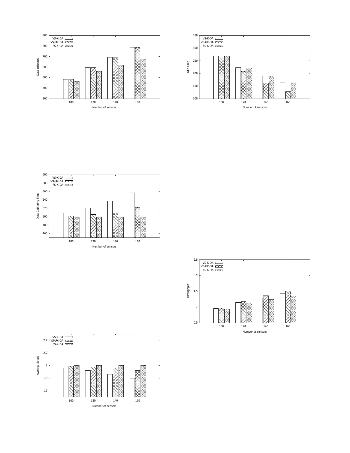
IEEE TRANSA CTIONS ON VEHICULAR TECHNOLOGY , V OL. XX, NO. XX, XXX 2019 1 Plane Sweep Algorithms for Data Collection in W ireless Sensor Netw ork using Mobile Sink Dinesh Dash Abstract —Usage of mobile sink(s) f or data gathering in wireless sensor networks(WSNs) impr oves the performance of WSNs in many respects such as power consumption, lifetime, etc. In some applications, the mobile sink M S travels along a predefined path to collect data fr om the nearby sensors, which are r eferred as sub- sinks. Due to the slow speed of the M S , the data delivery latency is high. Howev er , optimizing the data gathering schedule , i.e. optimizing the transmission schedule of the sub-sinks to the M S and the mov ement speed of the M S can reduce data gathering latency . W e formulate two novel optimization pr oblems for data gathering in minimum time. The first problem determines an optimal data gathering schedule of the M S by controlling data transmission schedule and the speed of the M S , where the data av ailabilities of the sub-sinks are given. The second problem generalizes the first, where the data availabilities of the sub- sinks are unknown. Plane sweep algorithms are proposed for finding optimal data gathering schedule and data availabilities of the sub-sinks. The performances of the proposed algorithms are evaluated through simulations. The simulation results reveal that the optimal distrib ution of data among the sub-sinks together with optimal data gathering schedule impr oves the data gathering time. Index T erms —Mobile sink, Data gathering pr otocol, Wir eless Sensor network, Plane Sweep Algorithm I . I N T RO D U C T I O N In WSNs, data generated at the sensor nodes are either transmitted through multi-hop transmission to a base station [8], [3], or a mobile sink ( M S ) moves through the commu- nication regions of the sensors and collects data from sensors directly/indirectly and brings them to a base station [9], [14]. In multi-hop transmission, sensors located near the base station are overloaded for relaying data from other sensors to the base station and are therefore prone to deplete their energy faster than other far aw ay sensors. Recently , mobile sink based data gathering has been gaining popularity significantly in wireless sensor networks (WSNs). In some applications, the MS periodically patrols the sensors, collects their data, returns to the base station and dumps the collected data at the base station. The problem of determining the tour of the M S has been studied rigorously in [9], [14], [4]. Mobile sink based data gathering improves the performance of WSNs in terms of energy consumption and lifetime of the sensors. Ho wever , introducing M S as a data carrier in the network increases the data deli very latency due to the slo w speed of the M S . Reducing the data deliv ery latency is a critical issue for the M S based data gathering. Ren and Liang et al. [17] have shown that the volume of data collection Dept. of CSE, National Institute of T echnology Patna, India, e-mail: dd@nitp.ac.in Manuscript recei ved XXX, XX, 2018; revised XXX, XX, 2019. is proportional to the data delivery latency . Time-sensiti ve applications such as forest fire detection, intrusion detection etc., demand time bound data deliv ery . Thus, improving data collection with minimum delivery latency is one of the most challenging issues in M S based data gathering. Sev eral data gathering algorithms are proposed to improve the data gathering time using mobile sink by shortening the tour length of the M S [9], [14], [4]. The data gathering time depends on the speed of the M S and the length of the tour . There are some studies in [18], [10] on the adaptiv e speed planning of M S along a predefined path. The M S adjust its speed to maximize network utility and minimize ener gy consumption. Data gathering problems for rechar geable sensor networks are formulated in [22], [ ? ], [ ? ] by jointly optimizing mobile data gathering and energy pro visioning. Gao et. al. [6], [7] propose novel data collection scheme, where a M S is moving along a predefined path with a fixed speed. But, the M S gets limited communication time to collect data from its nearby sensor nodes, referred as sub-sinks. Besides, a metaheuristic (genetic) algorithm is proposed to find data forwarding paths to improve the network throughput as well as to conserve energy . Due to the non-deterministic nature of the algorithm, the solution may vary each time you run the algorithm on the same instance. Therefore, the existing data gathering techniques using M S find optimal tour of M S or find data forwarding paths to M S to improv e the network performance, b ut there is a lack of studies on how to maximize data collection and minimize the data gathering time by controlling the data transmission schedule and speed of the M S . The data transmission schedule of the sub-sinks to the M S together with the speed schedule of the M S is called as data gathering schedule of M S . T o further improve the total data gathering time, we consider the above two factors and find an optimal distribution of the data generated within sensors among the sub-sinks. In addition, our algorithms are based on the geometric characteristics of the problem and are deterministic. Their correctnesses are also sho wn. An example of such type of network is illustrated in Figure 1. A mobile sink M S mov es along a gi ven path P . It collects pre-cached data from a few sensors which are directly reachable from the trajectory path P . Those directly reachable sensors are referred as sub-sinks ( ss 1 , ss 2 , ss 3 , ss 4 , ss 5 ). The M S may collect data from a sub-sink whenev er the M S comes under the communication range of the sub-sink. Thus, the sub-sinks send their data to the M S directly . The M S may be within multiple sub-sinks’ communication regions, and it receiv es data from any one of them at a time. Therefore, proper data transmission schedule of the sub-sinks are also required. The remaining sensors, which are not directly reachable to IEEE TRANSA CTIONS ON VEHICULAR TECHNOLOGY , V OL. XX, NO. XX, XXX 2019 2 P M S s 4 ss 2 s 6 s 9 ss 3 s 11 ss 4 s 7 s 8 s 3 s 1 ss 1 s 5 s 10 s 2 Mobile sink (MS) P ath for mobile sink Sensor Data forw arding link Sub-sink ss 5 Fig. 1. Example of P ath-constrained mobile sink based sensor network. M S ( e.g. s 1 , s 2 , . . . , s 11 ) send their data to the M S through the sub-sinks using multi-hop communication. The major challenges are to find the optimal data transmission schedule of the sub-sinks to the M S for their data deliv ery and speed variation of M S along P . Moreover , since a sensor can send data to M S through multiple sub-sinks, finding the optimal data distribution among the sub-sinks is another challenging issue in M S based data gathering. Our major contributions in this article are summarized as follo ws. 1) Introduce a time-sensitive data gathering problem using a speed adjustable mobile sink to collect data from sensor networks. 2) Linear programming formulation of the problem is dis- cussed, where the initial data availabilities of the sub- sinks are given. 3) Plane sweep based data gathering algorithm is proposed to collect data from the sub-sinks by controlling the data transmission schedule of sub-sinks and speed of the M S . 4) It is further generalized, where data a v ailabilities of the sub-sinks are optimized by controlling sensors’ data distribution among the sub-sinks to improve the data gathering time. The rest of the article is organized as follows. Section II dis- cusses some related works on data gathering problems. Section III presents system model and problem statement. Background and related terminologies are defined in section IV. Section V describes a plane sweep algorithm for data gathering in minimum time, where data av ailabilities of the sub-sinks are giv en. Section VI presents a plane sweep algorithm to improve the data gathering time by optimizing the data av ailability values of the sub-sinks so that the total data gathering time can be reduced. Section VII measures the performance of our proposed solutions. Finally , section VIII concludes the article. I I . R E L A T E D W O R K S Sev eral data gathering algorithms hav e been proposed in the literature using mobile sink M S where the path of the M S is controllable or fixed. Depending on applications, different objectiv es are attained such as maximizing network lifetime, minimizing the total energy consumption, reducing total tour length, etc. In this section, we classify the literature based on whether the path of the M S is controllable or fixed. Somasundara et. al. [19] claim that the sensors with higher variation in sensed data demand more frequent data collection than others. They proposed a solution based on optimizing trav elling path of the M S that allows the M S to visit sensor with a different frequency to reduce buf fer ov erflo w . They prov e that the decision version of the problem is NP-complete and two heuristic algorithms are proposed. The authors in [20] analyze various models of motion planning of mobile sink to solve mobile sink scheduling problem in order to minimize the data deliv ery latency of the network. He et. al. formulate the data gathering problem using M S as a trav elling salesman problem (TSP) with neighborhoods [9]. They schedule M S through the deployed region to improve the tour length of the M S and consider multi-rate wireless communication for data transmission. In [14], a periodic data gathering protocol is proposed for a disconnected sensor network. The M S trav erses the entire sensor network, polls sensors and gathers sensed data from sensors. It improves the scalability issue of large-scale sensor networks. Sayyed et al. in [18] inv estigate the utility of speed control mobile sink for collecting data in WSN. Single-hop clustering technique is used to increase the data collection rate as well as to decrease the data collection latency . T o overcome the delay due to the slow speed of the M S , a subset of sensors are selected as rendezvous nodes. These nodes are used to buf fer the data temporarily from the nearby sensors. When the M S visits these rendezvous nodes, then they transfer their data to the mobile sink. In [1], sensors are grouped into single hop clusters, and the mobile sink visits the centroids of these clusters. If the tour length of the set of centroids is greater than a given upper bound, then some of the clusters are remov ed until the tour length is less than the upper bound. In [2], a shortest path tree rooted at the initial position of the mobile sink is built, and then a sensor node having suf ficient energy as well as many nearby sensors within its vicinity is chosen as the next rendezvous node. In this way , a set of rendezvous nodes are selected and then a travelling salesman tour is obtained ov er the selected rendezvous nodes. In [11], k-means clustering with a weight function is used for finding the rendezvous points and an efficient tour among the rendezvous points is determined for the M S . In addition, an ef ficient data gathering scheme is also proposed to reduce the total packet drop. In [21], rendezvous nodes are selected using set covering problem. The M S tour is scheduled to pass through those rendezvous points. They introduce nov el rendezvous node rotation scheme for fair utilization of all the nodes. Konstantopoulos et. al. in [12] use multiple mobile IEEE TRANSA CTIONS ON VEHICULAR TECHNOLOGY , V OL. XX, NO. XX, XXX 2019 3 sinks to ensure timely deli very of data to the base station. Mobile sinks visit only a subset of rendezvous points while the remaining sensors forward their data to the rendezvous points through multi-hop communication. The proposed approach increases network lifetime by finding tour passing through energy-rich zones as well as through regions where energy consumption is high. In some scenarios, the trajectory of the M S is predefined to a fixed path. Ef ficient data collection algorithms are proposed to improve network performance. In [6], [7], data gathering algorithms are proposed for such cases to improve network performance. Data forwarding paths from the sensors to the sub-sinks are determined to maximize the data collection and balance the energy consumption. Huang et. al. in [10] consider a scenario where a label of importance is assigned to each sensing region. A path-constrained ground vehicle with adaptiv e speed is used to collect data from the sensing field. Although the approach tries to impro ve the data collection throughput, their speed control algorithms are reacti ve due to the adaptiv e nature of speed learning characteristics of the M S . Besides, these algorithms don’t ha ve any specific solution for controlling or optimizing the speed of the M S to improve the data collection rate and minimize delay . In article [ ? ], a deterministic algorithm is proposed for maximization of data collection using fixed speed mobile sink. Ho we ver , it may not provide quality data collection due to the mismatch between the data av ailable to the gatew ays and the data communication time between the gateways and M S . Maximizing the data collection throughput in rechargeable sensor networks is ad- dressed in [15]. Zhang et. al. [22] maximize data collection while maintaining the fairness of the network in rechargeable sensor networks. In [5], [13], data gathering protocols are proposed from path-constrained mobile sensors. The major drawback of the M S based system is its slow speed, which causes long data gathering delay . Since sensors have limited memory , it causes buf fer overflo w in the sensors. T o avoid buf fer overflo w , multiple mobile sinks are deployed and they periodically collect data from the mobile sensors and deliver the collected data to the base station. It can be noted that sev eral data gathering techniques hav e been proposed which focus on reducing the data gathering time of the mobile sink. The existing literature on path constrained mobile sink mostly consider efficient data forwarding mech- anism from the sensors to the mobile sink through the sub- sinks to improve the network performances. But, no existing works consider controlling the data transmission schedule of the sub-sinks to the M S along with the speed of the M S and the sensor’ s data distribution among sub-sinks to improve the total data collection and the total data gathering time of the mobile sink. I I I . S Y S T E M M O D E L A N D P RO B L E M F O R M U L A T I O N W e consider a wireless sensor network (WSN) which con- sists of a set of sensors N = { s 1 , s 2 , . . . , s n } . Sensor s i generates/senses DG ( s i ) amount of data from its en vironment. The communication topology of the network is modelled as an undirected graph G ( N , E ) . The communication regions of the sensors are modelled as disks. There is a mobile sink M S moving on a giv en path P . W e assume that the path P is approximated as piecewise straight line segments. The M S can mov e with a gi ven maximum speed value V to collect data from the sub-sinks. Ho we ver , the M S can change its speed depending upon the data av ailabilities of the sub-sinks. The M S can collect data from sensors whose communication disks intersect the path P . Based on the relati ve position of the sensors with respect to P , sensors are di vided into two groups, sub-sinks and far -aw ay sensors. Sensors which can directly communicate with M S on P are referred as sub-sinks and rest of the sensors are referred as far-away sensors. The far- away sensors send their data to M S through the sub-sinks. Let SS = { ss 1 , ss 2 , . . . , ss m } represent a set of sub-sinks which is a subset of N . Furthermore, we also assume that the M S and the sensors hav e sufficient energy and memory to collect and store all the sensed/relayed data temporarily . The data deliv ery capacity of a sub-sink is the amount of data that can be delivered by the sub-sink to the M S . The data deli very capacity of a sub-sink ss i depends on the time t i the M S allocates to ss i for its data deliv ery within the communication region of ss i and the data transmission rate dtr . W e assume that the M S can recei ve data from one sub-sink at a time. W e also assume that there is no data aggregation in the network. Then, our problems are stated as follows. Problem 1: Let the data availabilities of the sub-sinks be D A = { D A ( ss 1 ) , D A ( ss 2 ) , . . . , D A ( ss m ) } . Our objectiv e is to find data transmission schedule of the sub-sinks to the M S and a speed-schedule of the M S through P such that the M S can collect complete data from all the sub-sinks in minimum time. Our second problem generalizes the previous one, where data gathering time is further improved by optimizing the data av ailabilities of the sub-sinks. Problem 2: Find an optimal data av ailabilities of the sub- sinks D A = { D A ( ss 1 ) , D A ( ss 2 ) , . . . , D A ( ss m ) } by dis- tributing the sensors’ data among the sub-sinks along with their data transmission schedule to the M S and the speed- schedule of the M S through P such that the M S can collect complete data from all the sub-sinks in minimum time. I V . B AC K G RO U N D A N D T E R M I N O L O G I E S The far -away sensors send their data to the M S through the sub-sinks. A sub-sink generates its data and recei ves data from other sensors and store them temporarily in its local buf fer . This buffered data is deli vered by the sub-sink to the M S when it passes through the sub-sink’ s communication region. W e refer this b uf fered data as data availability of the sub-sink. Since the maximum speed V of the M S is giv en, a naiv e approach for the M S is to move at this maximum speed V on P and visit all the sub-sinks and collect their data. But it may not collect complete data from all the sub-sinks. Ho wev er, if the speed of the M S can be varied according to the data av ailabilities of the sub-sinks, then it may improv e the amount of data collection. For instance, the M S should mov e at slow speed within the communication range of a sub-sink, which has more IEEE TRANSA CTIONS ON VEHICULAR TECHNOLOGY , V OL. XX, NO. XX, XXX 2019 4 P Sub-sink’s communication disk Path P distance speed Speed sc hedule (a) (b) S E Fig. 2. Speed-schedule of mobile sink in sensor network data, whereas it should move at a faster speed within the communication range of a sub-sink which has less or no data. Furthermore, the M S should mov e with its maximum speed of V , when it is not under the communication range of any sub- sink or the sub-sinks do not have data to deliver . Determining the speed of the M S at different position on P is referred as speed-schedule of M S . Note that the speed of the M S can vary between 0 to V . It may happen that the M S is within multiple sub-sinks communication regions then one of the sub-sinks can transmit data to the M S . Therefore, proper time sharing among the sub-sinks is also required. W e refer it as data transmission schedule of the sub-sinks. The data transmission schedule of the sub-sinks to the M S together with the speed schedule of the M S is called as data gathering schedule of M S . Our objectives are to find optimal data gathering schedule of the M S through the communication regions of the sub-sinks along the path P to collect complete data from the sub-sinks in minimum time. A possible speed-schedule for M S is shown in Figure 2. Figure 2(a) sho ws the path P of the M S with dashed line and circles denote the communication disks of the sub-sinks. Let the M S start from S and end at E while travelling through the path P . Figure 2(b) sho ws the speed-schedule of the mobile-sink at different position on P . It shows that the speed of M S is slo w within the communication disks of the sub-sinks whereas it runs with its maximum speed V outside the communication disks. W e introduce some terminologies to describe our algorithm, which are as follows. Definition 1. Start-point ( p s i ) : It is a first point on P fr om which a sub-sink ss i can communicate or start delivering data to the M S . Definition 2. End-point ( p e i ) : It is a last point on P after which a sub-sink ss i cannot communicate or ends delivering data to the M S . Definition 3. Data av ailability ( DA ( ss i ) ) : It is the amount of data available at a sub-sink ss i . Definition 4. Data deliv ery time ( DT ( ss i ) ) : It is the minimum time requir ement to transmit the data available at a sub-sink ss i to the M S . Data deli very time is determined using D T ( ss i ) = DA ( ss i ) dtr S p s 1 p e 1 p s 2 p s 3 p s 4 p s 5 p e 2 p e 3 p e 4 p e 5 p s 1 p e 1 p s 2 p s 3 p s 4 p s 5 p e 2 p e 3 p e 4 p e 5 ss 1 ss 2 ss 3 ss 4 ss 5 E S E (a) (b) Fig. 3. Start-point and end-point of sub-sinks on path P formula, where dtr denotes the data transmission rate between ss i and M S . V . D A T A G A T H E R I N G I N M I N I M U M T I M E ( DAT A A V A I L A B I L I T Y O F S U B - S I N K S A R E K N O W N A P R I O R I ) In this section, we first discuss linear programming problem (LPP) formulation of the proposed problem, thereafter we discuss a plane sweep based algorithm. The mobile sink M S trav els through the path P and collects complete data from all the sub-sinks. The data av ailability v alues of the sub-sinks are giv en. The M S recei ves data from one sub-sink at a time. The objectiv e is to collect the complete data from all the sub-sinks in minimum time. W e control the data gathering schedule of the M S . In other words, the time allocation of the M S to the sub-sinks and the time spent by the M S within their communication regions are determined based on their data av ailability values to minimize the data gathering process. A. LPP F ormulation The ordering of the start-points and end-points of the sub- sinks partition the path P into disjoint segments/interv als. An example of partitioning the path P into segments is shown in Figure 3. In Figure 3(a), a set of sub-sinks SS = { ss 1 , ss 2 . . . ss 5 } and their start-points and end-points are shown on the path P . The ordering of the start-points and end-points of the sub-sinks partition the path P into disjoint segments, which are shown in Figure 3(b). Zero or more sub- sinks are reachable to the M S from a particular segment. The idea of the solution is that the data gathering time within each segment is shared properly among the sub-sinks such that the M S can collect complete data from all the sub-sinks through the segments and total data gathering time from the starting position S to the ending position E is minimum. Also, the M S maintains the maximum speed limit constraint. The start-points and end-points of the sub-sinks partition the path P into disjoint segments/interv als. The m sub-sinks hav e 2 m end-points. This will partition the path P into at most 2 m + 1 disjoint segments { I 1 , I 2 , . . . I 2 m +1 } . For each segment, we use a set of variables for the set of sub-sinks reachable from the segment. W ithin a particular segment I j , the set of sub-sinks reachable to the M S remains unchanged. Let S S ( I j ) denote the sub-sinks in SS reachable to the M S within the se gment I j . Let t i j denote the time allocated to sub-sink ss i ∈ S S ( I j ) for transferring its data to the M S IEEE TRANSA CTIONS ON VEHICULAR TECHNOLOGY , V OL. XX, NO. XX, XXX 2019 5 on the segment I j . If a segment I j is not reachable to any sub-sink, then we assume that it is reachable from a virtual sub-sink ss 0 which has no data, i.e. D A ( ss 0 ) = 0 , and the time the M S spends to cross the segment I j is denoted by T ( I j ) = t 0 j ≥ | I j | V . Similarly , if from segment I j two sub- sinks ss i and ss k are reachable, i.e. S S ( I j ) = { ss i , ss k } , then there are two variables t i j and t k j corresponding to two sub-sinks for the segment I j . Each variable value denotes the amount of time allocated to the corresponding sub-sink for data deli very when the M S trav els through the segment I j . There are two types of constraints (i) time spent on each segment I j by the M S is at least the travelling time | I j | V , and (ii) total time t i = P 2 m +1 j =1 t i j : ss i ∈ S S ( I j ) , allocated by the M S to a sub-sink ss i for its data deliv ery , must be greater than or equal to the sub-sink’ s data deli very time D T ( ss i ) . The LPP formulation of the said problem is shown in Equation 1. Minimize : 2 m +1 X j =1 X i : ss i ∈ S S ( I j ) t i j Subject to : X i : ss i ∈ S S ( I j ) t i j ≥ | I j | V , j = 1 . . . (2 m + 1) X j : ss i ∈ S S ( I j ) t i j ≥ DT ( ss i ) , i = 1 . . . m t i j ≥ 0 , i = 0 . . . m, j = 1 . . . (2 m + 1) (1) After solving the LPP in Equation 1, t i j , i = 0 . . . m, j = 1 . . . (2 m + 1) are kno wn, which denote the data transmission schedule of the sub-sinks. The lengths of the segments I i , i = 1 . . . (2 m + 1) are already deri ved from the start-points and end-points. Hence, the speed of the M S at dif ferent segments can be determined easily . The following subsection discusses a plane sweep based algorithm for the problem. B. Plane Sweep Algorithm The mobile sink M S moves through the path P . When the M S is within the multiple sub-sinks’ communication range, then the M S recei ves data from only one of them by prioritizing them according to their end-points positions on P . The sub-sink whose end-point appears first on P has higher priority than that sub-sink whose end-point appears later . Let P R ( ss i ) denote the priority of a sub-sink ss i . In the plane sweep algorithm, it is simulated by moving a sweep line through the path P . W e consider a horizontal data gathering path P for the M S and a virtual vertical line perpendicular to P , called sweep line moves (sweeps) through the path P from S to E . While sweeping the sweep line intersects the sub-sinks’ communication disks. W e hav e defined two types of ev ents : start-point event and end-point ev ent for ev ery sub-sink. Start-points and end-points of the sub-sinks are stored in an event queue Q according to their appearance on P from left to right. At a particular position of the sweep line on P , we maintain a list of sub-sinks in a status line data structure L . The sub-sinks whose communication disks intersect the sweep line on P are in L . At a particular position on P , if multiple sub-sinks’ communication disks intersect the sweep line on P and they hav e data, then a sub- sink ss i in L with maximum priority gets the preference to deliv er data to M S . Initially , all the start-points and end-points of the sub- sinks are added to the event queue Q . W e are calling three methods to perform dif ferent operations on the e vent queue Q . I nser tI nQ () method is used for inserting an ev ent, Remov eF r omQ () method remov es the leftmost event on P , and P eek F r omQ () method retriev es the leftmost ev ent but does not remov e it from the queue. Similarly , three methods I nser tI nL () , R emoveF romL () , and P eekF romL () are used to perform three dif ferent operations on the status line data structure L . Events are processed one by one from the ev ent queue Q , as the sweep line moves through the path P . The top ev ent is removed from Q and is referred as current ev ent C E . A sub-sink ss i is inserted into L , whene ver the sweep line processes its start-point p s i . If the sweep line is processing an end-point p e i of sub-sink ss i and the complete data of ss i is not yet deli vered, then the M S waits at the end-point p e i and receiv es the remaining data from ss i . Subsequently , the sub-sink ss i is removed from L . Thereafter , the next event point N E is picked from the ev ent queue Q . Tra vel time T T of the M S between current e vent C E and the next event N E is determined assuming that the M S mov es with its maximum speed V in between the two events. Thereafter , maximum priority sub-sink ss j is picked from L . If the data transmission time D T ( ss j ) of the sub-sink ss j is ≤ T T , then the sub-sink ss j completes data delivery to the M S between the two events. The sub-sink ss j is removed from L . Subsequently , the next highest priority sub-sink in L is picked for data deli very . This process continues until the sweep line reaches another ev ent point or the data deliv ery process is completed. If there is no sub-sink in L having data to deliver then the M S moves with its maximum speed V . The detailed algorithm is presented in Algorithm 1. In Figure 3(a), the M S starts its journey from S with speed V . As it reaches p s 1 , then the sub-sink ss 1 is inserted into L . Thereafter , M S starts recei ving data form ss 1 until it reaches p s 2 . If the data deli very of ss 1 is not ov er , then there are two sub-sinks ss 1 , ss 2 reachable to M S within segment [ p s 2 p e 1 ] . As the end-point p e 1 appears before p e 2 , therefore, according to our algorithm, sub-sink ss 1 gets the pri vilege to deliv er its remaining data to M S within the segment [ p s 2 p e 1 ] . If the data deliv ery of ss 1 is still not o ver within | p s 1 p e 1 | V time, then the M S waits at point p e 1 for the remaining data deliv ery time for the duration of D T ( ss 1 ) − | p s 1 p e 1 | V time. Otherwise, the M S starts receiving data from ss 2 after crossing the start-point p s 2 and allocating D T ( ss 1 ) time to ss 1 . In this way , the M S either mov es with its maximum speed or waits at the end-points of the sub-sinks until it reaches the end of the path E . Corollary 1. Data gathering sub-paths of the mobile sink M S on P from a sub-sink ss i is confined within [ p s i , p e i ] for i ∈ { 1 . . . m } . Theorem 1. If the mobile sink M S follows the Algorithm 1 for data gathering, then it r eceives complete data fr om all the sub-sinks. IEEE TRANSA CTIONS ON VEHICULAR TECHNOLOGY , V OL. XX, NO. XX, XXX 2019 6 Algorithm 1: Plane sweep algorithm for data gathering using M S Data: Location( ss i ) and D A ( ss i ) ∀ ss i ∈ SS , P , V , dtr Result: Data Transmission Schedule of the sub-sinks, and Speed Schedule of M S ∀ ss i ∈ SS : Compute start-point ( p s i ) and end-point ( p e i ) with respect to P ; Q = ∅ , m = | SS | ; / * Initialize event queue Q with start-points and end-points * / for i = 1 to m do InsertInQ( p s i ); InsertInQ( p e i ); D T ( ss i ) = DA ( ss i ) dtr ; / * Data delivery time of ss i * / end L = ∅ ; / * Initialize status line L * / The M S moves with its maximum speed V from S to the next end-point e vent, or until it reaches end of the path E ; while Q 6 = ∅ do C E = Remov eF r omQ () ; if C E = p s i then InsertInL( ss i ) ; else if C E = p e i ∧ DT ( ss i ) > 0 then M S stops and recei ves remaining data of ss i ; D T ( ss i ) = 0 ; Remov eFromL( ss i ) ; / * If L 6 = ∅ then select a sub-sink ss j with maximum priority from L and M S starts receiving data from ss j * / N E = P eek F r omQ () ; / * next event * / T T = dist ( C E ,N E ) V ; / * travel time between C E and N E * / ss j = P eek F r omL () ; while L 6 = ∅ ∧ D T ( ss j ) ≤ T T do M S moves with speed V and recei ves data from ss j for DT ( ss j ) time ; T T = T T − D T ( ss j ) ; D T ( ss j ) = 0 ; Remov eF r omQ ( p e j ) ; Remov eF r omL ( ss j ) ; ss j = P eek F r omL () ; end if L 6 = ∅ ∧ D T ( ss j ) > T T then D T ( ss j ) = D T ( ss j ) − T T ; M S moves with speed V and continue recei ving data from ss j for T T time ; else M S moves with speed V without recei ving any data to next e vent for T T time ; end Pr oof. Algorithm 1 selects the highest priority sub-sink in L for data deliv ery to the M S . A sub-sink ss i ∈ SS is remov ed from L only when the M S finishes receiving its data by allocating D T ( ss i ) time to ss i . The time allocation may be continuous or discontinuous. A sub-sinks ss i is inserted to L whenev er the M S crosses p s i . Since all the star -points and end- points of the sub-sinks are in Q and are processed. Therefore, all the sub-sinks get a chance to be in L . Once the algorithm ends then the e vent queue Q and the list L become empty . Therefore, all the sub-sinks must have deli vered their complete data to the M S . Theorem 2. The mobile sink M S completes the data gather- ing pr ocess in minimum time by following Algorithm 1. Pr oof. Assume for the sake of contradiction that the M S does not complete the data gathering process in minimum time. According to our algorithm, the M S mov es with its maximum speed V throughout the path except at some end-points. So, there is an extra delay at some end-points. Extra delay for receiving data from a sub-sink ss i is possible only when the M S waits at p e i , but for some sub-path of [ p s i , p e i ] , the M S mov es without receiving data from any sub-sink or recei ves data from a sub-sink ss j , whose end-point p e j appears after p e i . This is because the sub-sinks, whose end-points appear after p e i can deliver data beyond [ p s i , p e i ] , and may overall reduce the waiting time at p e i . According to Algorithm 1, once the M S enters [ p s i , p e i ] , it either receiv es data from ss i , or any other sub-sink ss j such that P R ( ss j ) ≥ P R ( ss i ) in L . This implies p e j appears before p e i . Therefore, there is no sub-path within [ p s i , p e i ] where the M S moves/w aits without receiving data from any sub- sink ss j ∈ L , where P R ( ss j ) ≥ P R ( ss i ) and waits at p e i . Hence, the M S does not mak e e xtra delay at any end-point and completes the data gathering process in minimum time. Theorem 3. T ime complexity of the plane sweep algorithm 1 is O ( m log m ) . Pr oof. Throughout the algorithm, an event point (start- point/end-point) of a sub-sink is inserted once and remov ed once in the event queue Q , and in total 2 m e vent points are processed. The events are processed from event queue Q using a heap data structure. Inserting and then removing the ev ent points require O ( m log m ) time. During the processing of an e vent, some basic operations on the status line data structure L are performed. In the worst case, m sub-sinks are simultaneously in L . Therefore, the time needed to perform an insert or delete operation on the status line is O (log m ) and the peek operation takes O (1) time. The plane sweep algorithm processes 2 m event points for m sub-sinks. In total m insert and m delete operations, and at most 2 m peek operations are performed on the status line data structure L , and each such operation takes at most O (log m ) time. Hence, it follows that the total time processing all the ev ents is O ( m log m ) . IEEE TRANSA CTIONS ON VEHICULAR TECHNOLOGY , V OL. XX, NO. XX, XXX 2019 7 V I . I M P RO V IN G T H E D AT A G A T H E R I N G T I M E B Y O P T I M I Z I N G T H E D A TA A V A I L A B I L I T I E S O F T H E S U B - S I N K S The solution in the previous section finds a data gathering schedule of the M S , where the data av ailability v alues of the sub-sinks are given. This section generalizes the problem, where data a v ailabilities of the sub-sinks are determined to improv e the data gathering time. Proper distribution of the sensors’ data among the sub-sinks is carried out to improve the data gathering time. Determining an optimal data distribution among the sub-sinks is another challenging issue in WSN. The data av ailability values of the sub-sinks are determined using a plane sweep algorithm for the given sensor network. After determining the optimal data a vailability values of the sub- sinks, we consider the values as data deli very capacity of the sub-sinks and the sensors’ data are pushed to those sub-sinks using network flo w algorithm. Thereafter , Algorithm 1 is used to complete the data gathering process in minimum time. In summary , this section discusses the solution for the Problem 2, where our objective is to distribute the sensors’ data among the sub-sinks properly so that the M S can collect complete data from all the sub-sinks in minimum time. A. Determining Data A vailabilities of the Sub-Sinks Using Plane Sweep Algorithm In this subsection, we determine the data availability v alues of the sub-sinks for a gi ven network topology . W e assume that the data generated on the sensors are known, which are denoted as D G ( s i ) : i = 1 : n . Using a plane sweep algorithm, we determine the data availability v alues of the sub-sinks D A ( ss i ) : i = 1 : m . Initially , the sensor network is parti- tioned into connected components C = { c 1 , c 2 , . . . c k } based on its communication topology G . The idea of this algorithm is that the data generated in a component is distributed among its corresponding sub-sinks so that the M S can collect complete data from the component through its sub-sinks in minimum time. The M S moves with its maximum speed V through P , except at a fe w end-points. For individual connected component, the total data gen- erated by the sensors in the corresponding component is determined. Let { D G ( c 1 ) , D G ( c 2 ) , . . . D G ( c k ) } denote the data generated in the components. The data a vailabilities of the sub-sinks are initialized to zero : D A ( ss 1 ) = 0 , D A ( ss 2 ) = 0 , . . . D A ( ss m ) = 0 . The start-points and end-points of the sub-sinks are determined. The sub-sinks are labelled with their corresponding component identity . Let C ( ss i ) denote the component identity of a sub-sink ss i . The last sub-sink of a component c i denoted by LS S ( c i ) is a sub-sink, whose end- point appears last on P among all the sub-sinks in c i . For each component c i , identify its last sub-sink LS S ( c i ) . The start-points and end-points of the sub-sinks are stored in an ev ent queue Q according to their order on the path P . The status line data structure L is initialized to ∅ . A virtual perpendicular sweep line moves through the path P and process the e vents one after another from the ev ent queue. At a particular position on the path P of the sweep line, it keeps track of all the sub-sinks in a status line L , whose communication disks intersect the sweep line on the path P . The priority of a sub-sink ss i in L is based on the two parameters : its corresponding component’ s last sub-sink’ s end-point position, i.e. end-point of LS S ( ss i ) , and its start- point p s i on P . If two sub-sinks ss i and ss j belong to same component, i.e. C ( ss i ) = C ( ss j ) , then the sub-sink whose start-point appears first on P , has higher priority than the other sub-sink. If the two sub-sinks belong to different components, i.e. C ( ss i ) 6 = C ( ss j ) and the end-point of LS S ( C ( ss i )) appears before the end-point of LS S ( C ( ss j )) on P , then P R ( ss i ) > P R ( ss j ) . The top event is remov ed from the queue Q and is referred as the current e vent C E . If C E is a start-point of ss i , then ss i is inserted into L . If C E is an end-point of sub-sink ss i and it is the last sub-sink of its corresponding component c j and the component has data ( D A ( c j ) > 0 ) then the data av ailability of ss i is increased by D A ( c j ) . Subsequently , the sub-sink ss i is removed from L . Thereafter , the next event point N E is picked from the ev ent queue Q . T ravel time T T of the M S between current e vent C E and the next ev ent N E is determined assuming that the M S mo ves with its maximum speed V in between the two ev ents. Next, the maximum priority sub-sink ss j is picked from L . Let C ( ss j ) denote the component of sub-sink ss j . If the remaining data av ailability of the component C ( ss j ) , which is D A ( C ( ss j )) ≤ T T ∗ dtr (data transmission capacity of ss j between the two ev ent points), then data a v ailability of ss j is increased by D A ( C ( ss j )) . The sub-sink ss j is removed from L . The remaining travel time between the two events C E and N E of the M S is updated accordingly . This process continues until the remaining travel time by the M S is exhausted and subsequently process the next e vent. In other words, if data transfer from a component c i is over before the sweep line reaches the end-point of its corresponding last sub-sink LS S ( c i ) , then all the sub-sinks in c i are removed from L . This process continues until the sweep line reaches the next ev ent point or the data deli very process is completed. The detailed algorithm for finding data a v ailabilities of the sub- sinks is shown in Algorithm 2. Theorem 4. T ime complexity of the plane sweep algorithm 2 is O ( n + e + m log m ) , where n and e denote the number of sensors and number of links in the communication graph G . Pr oof. Depth first search is used for partitioning the network into components which can be performed in O ( n + e ) time. Computing total data generated for each component can be performed in O ( n ) time. Finding the start-points and end- points of the sub-sinks can be done in O ( m ) time. Identifying the last sub-sink for each component can be done in O ( n ) time. The time complexity analysis for the rest of the algorithm is similar to Algorithm 1. The plane sweep algorithm processes 2 m event points. The ev ents are inserted and then remov ed from the event queue, which takes overall O ( m log m ) time. During the processing of an ev ent, some basic operations on the status line data structure are performed. There are at most m sub-sinks intersecting the sweep line on P at any time and therefore, the time needed to perform an insert or delete IEEE TRANSA CTIONS ON VEHICULAR TECHNOLOGY , V OL. XX, NO. XX, XXX 2019 8 Algorithm 2: Plane sweep algorithm for computing data av ailabilities of the sub-sinks Data: Communication topology G, Data generated by the sensors { DG ( s 1 ) , D G ( s 2 ) , . . . D G ( s n ) } , SS , P , V , dtr Result: Data av ailabilities of the sub-sinks D A = { D A ( ss 1 ) , D A ( ss 2 ) , . . . D A ( ss m ) } Partition the sensor network into components C = { c 1 , c 2 , . . . c k } based on its communication topology ; ∀ c i ∈ C : Compute total data generated DG ( c i ) by adding all sensors data in the component ; ∀ c i ∈ C : DA ( c i ) = D G ( c i ) ; ∀ ss i ∈ SS : D A ( ss i ) = 0 ; ∀ ss i ∈ SS : Find start-point ( p s i ), end-point ( p e i ) and component-id C ( ss i ) ; ∀ c i ∈ C : Find last sub-sink LS S ( c i ) ; / * Initialize event queue Q with start-point and end-point of the sub-sinks * / Q = ∅ , m = | SS | ; for i = 1 to m do InsertInQ( p s i ); InsertInQ( p e i ); end L = ∅ ; / * Initialize status line L * / while Q 6 = ∅ do C E = Remov eF r omQ () ; if C E = p s i then InsertInL( ss i ) ; else if C E = p e i then if ss i ∈ c j ∧ ss i = LS S ( c j ) ∧ D A ( c j ) > 0 then D A ( ss i ) = D A ( ss i ) + D A ( c j ) ; D A ( c j ) = 0 ; Remov eFromL( ss i ) ; N E = P eek F r omQ () ; Let dist(CE,NE) = Distance between e vents C E and N E ; T T = dist ( C E ,N E ) V ; / * Travel time between C E and N E * / ss j = P eek F r omL () ; / * Peek maximum priority sub-sink in L * / while L 6 = ∅ ∧ DA ( C ( ss j )) ≤ T T ∗ dtr do D A ( ss j ) = D A ( ss j ) + D A ( C ( ss j )) ; D T T = DA ( C ( ss j )) dtr ; / * Data transfer time * / T T = T T − D T T ; D A ( C ( ss j )) = 0 ; Remov eF r omQ ( p e j ) ; Remov eF r omL ( ss j ) ; ss j = P eek F r omL () ; end if L 6 = ∅ ∧ DA ( C ( ss j )) > T T ∗ dtr then D A ( ss j ) = D A ( ss j ) + T T ∗ dtr ; D A ( C ( ss j )) = D A ( C ( ss j )) − T T ∗ dtr ; end s 4 ss 2 s 6 s 9 ss 3 s 11 ss 4 s 7 s 8 s 3 s 1 ss 1 s 5 s 10 s 2 P ss 5 c 1 c 2 Fig. 4. Connected components corresponding to the sensors network operation on status line is O (log m ) and peek operation can be performed in O (1) time. Through the algorithm, a sub- sink is inserted once and remov ed once from the status line data structure. Therefore, the total time spent on accessing the sweep line status data structure is O ( m log m ) . Hence, it follows that the total time spent processing all the ev ents is O ( m log m ) . Therefore, the total time complexity of the algorithm is O ( n + e + m log m ) B. Distributing Data Among the Sub-Sinks Using Network Flow Algorithm Once the data av ailability values of the sub-sinks D A ( ss 1 ) , D A ( ss 2 ) . . . D A ( ss m ) are determined using Algo- rithm 2, this phase distrib utes the sensors’ data among the sub-sinks. Data are pushed from the sensors to the sub-sinks based on their calculated data av ailability v alues. Sensors use the communication topology network to send data to the sub- sinks. Network flow algorithm is used for finding data flo w from the sensors to the sub-sinks. Construction of network flow graph and determining the distribution of data from the sensors to the sub-sinks for a giv en communication topology is described with an example for the sensor network in Figure 1. The connected components corresponding to the sensor network of Figure 1 are identified and labelled with c 1 , and c 2 in Figure 4. T o determine the data distribution from the sensors to the sub-sinks, a network flow graph is constructed using the communication topology of the sensor network. Thereafter , the sensors’ data are distributed among the sub-sinks based on the data av ailability v alues of the sub-sinks, the amount of data generated within the sensors, and the communication topology . The network flo w graph corresponding to the communication topology in Figure 4 is shown in Figure 5. A virtual source verte x V S and a virtual sink verte x V K are added to the network topology . T o maintain the cleanness of the figure, we IEEE TRANSA CTIONS ON VEHICULAR TECHNOLOGY , V OL. XX, NO. XX, XXX 2019 9 V K s 4 ss 2 s 6 s 9 ss 3 s 11 ss 4 s 7 s 8 s 3 s 1 ss 1 s 5 s 10 s 2 Virtual Sink (VK) Virtual link Virtual Source (VS) V S V S V S V S ss 5 Fig. 5. Network flo w graph corresponding to the sensors network; Link capac- ity : ( V S, s i ) = DG ( s i ) ; ( V S, ss i ) = DG ( ss i ) ; ( ss i , V K ) = D A ( ss i ) ; other links capacities are ∞ hav e drawn four duplicate virtual source vertices, b ut actually they are a single verte x V S . The virtual source vertex is incident to the sensor nodes including the sub-sinks using virtual links. The capacities of these virtual links are set based on their data generation capacities. Therefore, the capacity of a link between V S and s i is DG ( s i ) . Similarly , the link capacity between V S and ss i is D G ( ss i ) because, as these are data generation limits of the sensor s i /sub-sink ss i . The sub-sinks are incident to the virtual sink V K through virtual links. The capacity of a virtual link between a sub-sink ss i and the virtual sink V K is set to DA ( ss i ) , which is its data av ailability value determined in the previous phase. Other links represent the communication links among the sensors/sub-sinks, and their capacities are set to infinity because we assume that a sensor can forward the data generated within itself or receiv ed from its neighbors. Thereafter , the network flow algorithm is used for finding the maximum data flo w from the V S to V K . The flo w value of the links denotes the data flow between the corresponding sensors/sub-sinks. Finally , data is delivered from a sub-sink to virtual sink V K . The flow value between a sub-sink and the virtual sink denotes the actual data deli very by the sub-sink to the M S . C. Gathering Data Using Algorithm 1 In this subsection, we find an optimal data gathering sched- ule of the mobile sink ( M S ) to collect complete data from all the sub-sinks in minimum time. Once the data av ailabilities of the sub-sinks D A ( ss 1 ) , D A ( ss 2 ) . . . D A ( ss m ) are deter- mined, and data are pushed from the sensors to the sub-sinks, we use the Algorithm 1 of Section V to find the data gathering schedule of the M S . Theorem 5. If the data availabilities of the sub-sinks are determined using Algorithm 2 and M S follows the speed- schedule using Algorithm 1, then the mobile sink M S com- pletes the data gathering pr ocess in minimum time. Pr oof. The data a vailabilities of the sub-sinks are determined using Algorithm 2 such that the M S is able to receiv e com- plete data from a component while moving with its maximum speed V and if required waits only at the last sub-sink’ s end- point. The data generated in the sensors are distributed among its sub-sinks based on the data av ailability values determined using Algorithm 2. According to Algorithm 1, while the M S is moving, it receives data from the highest priority sub-sink having data to deliver . Let the first sub-sink of a component c i be a sub-sink ss j ∈ c i , whose start-point p s j appears first on P . Let c s i = p s j denote the start-point of the first sub-sink of c i . Similarly , c e i denotes the end-point of the sub-sink LS S ( c i ) . Algorithm 2 prioritizes the sub-sinks based on their compo- nents’ last sub-sink’ s end-point positions and sub-sinks’ start- point positions. The sub-sink whose component’ s last sub- sink’ s end-point appears first on P , gets the highest preference for data deli very . If two sub-sinks are on the same component, then the sub-sink whose start-point appears first has a higher priority than the other . The M S recei ves data from a sub-sink in L , which has maximum priority and has data to deliv er . If there is no data, then it is immediately remov ed from L . Similar to the proof of Theorem 2, assume for the sake of contradiction that the M S does not complete the data gathering process in minimum time. It implies that there is a sub-path of [ c s i , c e i ] for component c i , and the sub-path is under the communication disk of a sub-sink ss k ∈ c i , where the M S mov es without receiving data from any sub-sink or recei ves data from a sub-sink ss l , whose priority P R ( ss l ) < P R ( ss k ) and the M S waits at c e i for receiving data from component c i . The sub-sink ss l may belong to (i) same component c i as of ss k , or (ii) in a dif ferent component c j , i.e. c j 6 = c i . In case (i), where sub-sink ss l ∈ c i , the M S does not wait at c e i . This is because within the communication disk of ss k , if the M S receiv es data from sub-sink ss l ∈ c i with P R ( ss l ) < P R ( ss k ) , then all the sub-sinks in c i with priority ≥ P R ( ss k ) do not hav e data to deliv er . In case (ii), where sub-sink ss l ∈ c j and c j 6 = c i , based on the first sub-sink’ s start-point and last sub-sink’ s end-point positions of a component, two components c i and c j hav e three different types of ov erlaps as shown in Figure 6. All other types of overlaps are equiv alent to one of them. W e will show that extra delay at c e i does not hold for any of these three types of overlaps. In Figure 6(a) type overlap, two components are disjoint. Hence, the M S does not recei ve data from ss l ∈ c j within [ c s i , c e i ] and make an extra delay at c e i . In Figure 6(b) type ov erlap, the second component starts before the end of first component. In this case, the priority of any sub-sink in component c i is higher than any sub-sink in component c j . Hence, the M S recei ves data from ss l ∈ c j within [ c s i , c e i ] only when there is no data in ss k . If there is no data in ss k , then all data from c i is already delivered to the M S and the M S does not wait at c e i . IEEE TRANSA CTIONS ON VEHICULAR TECHNOLOGY , V OL. XX, NO. XX, XXX 2019 10 c s i c e i c s i c e i c s i c e i (a) (b) (c) c s j c e j c s j c e j c s j c e j Fig. 6. Overlaps between components In Figure 6(c) type overlap, the priority of any sub-sink in component c j is higher than any sub-sink in component c i . So, P R ( ss l ) can not be less than P R ( ss k ) . Therefore, in both case (i) and case (ii) our assumption does not hold and hence the theorem is proved. V I I . E X P E R I M E N T A N D P E R F O R M A N C E A N A L Y S I S W e ev aluate the performance of our two proposed algo- rithms. W e have used MA TLAB for implementing our al- gorithms. In this section, we ev aluate the performances of our proposed algorithms. W e refer the algorithms for data gathering algorithm using speed controllable mobile-sink with known data av ailability (Algorithm 1) as VS-K-D A . VS-UK- D A refers to the case where data av ailabilities of the sub-sinks are unknown and optimized using Algorithm 2. Algorithm VS-UK-D A is combined with network flow algorithm for data distribution and with Algorithm 1 to find data gathering schedule. W e compare the above two algorithms with a third algorithm FS-K-D A , where data av ailabilities of the sub-sinks are known apriori as in VS-K-DA and the mobile sink M S is moving with its maximum speed as in [7] for collecting data from the sub-sinks. A. Simulation en vironment During simulation, the number of sensor nodes is varying for 100, 120, 140 and 160. The communication range of sen- sors is set to 75m. Sensors deployment region is a rectangular area of size 1000m x 400m. The rectangular region is vertically partitioned into four sub-regions of length 250m each. W ithin each sub-region of length 250m, sensors are randomly de- ployed within a vertical strip of [75m : 150m]. This is done to ensure that the random communication topology forms at least four connected components and there are gaps between the consecutiv e components. In the simulation, the M S is moving along a horizontal path P at the centre of the region (y=200m). The maximum speed V of the M S is set to 2 m/s. The M S collects data from one sub-sink at a time, which is within the communication range. The data transfer rate between a sub-sink and the M S is set to 2 Kbps. W e assume that the sensors generate data randomly between 0 to 10 packets, and each packet is of size 1Kb. The far-a way sensors send their sensed data to the sub-sinks through multi-hop forwarding. Data av ailabilities of the sub-sinks (for kno wn apriori case) of problem 1 is determined using shortest path routing, where the sensors forward their data to its closest (hop-count) sub-sink. Let e r and e t denote energy consumption for receiving and transmitting unit bit data. Let E i represent the total energy consumption of a sensor s i for receiving d i r bits, and transmitting d i t bits. Therefore, E i can be written as : E i = ( e r ∗ d i r + e t ∗ d i t ) (2) T otal energy consumption of the network E total is calcu- lated as the summation of energy consumption for forwarding data from the sensors to the M S through their respectiv e sub- sinks. E total = n X i =1 E i (3) Let D D ( ss i ) denote data deli vered by a sub-sink ss i to the M S . Hence, total energy consumption E total includes energy consumption for deli vering data from the sub-sinks to the M S , which is P m i =1 e t ∗ D D ( ss i ) . This is because the sub-sinks SS ⊆ N . T able I summarizes the simulation parameters. T ABLE I S I MU L A T IO N P AR A M E TE R S Parameter V alue Rectangular deployment area 1000m × 400m No. of sensors 100, 120, 140, 160 Maximum speed of M S 2 m/s Communication range of sensor 75 m Data transmission rate 2 Kbps e r 2 µ Joule/bit e t 3 µ Joule/bit B. P erformance analysis of the proposed algorithms Figure 7 shows the total data collected by the mobile-sink with respect to the number of sensors. From the figure, it is obvious that the amount of data collection is proportional to the number of sensors. Data collection in VS-K-D A and VS- UK-D A are same because both the algorithms collect complete data from the network, whereas data collection in FS-K-DA is lesser than the two proposed algorithms. The difference be- tween fixed speed and v ariable speed data gathering increases as the number of sensors increases. This is because, in VS- K-D A and VS-UK-D A , the complete data from the sub-sinks are collected by controlling the speed of the M S , whereas in FS-K-DA , the M S mo ves with its maximum speed, and the sub-sinks do not get enough time to deliver their data completely . Figure 8 shows the data gathering time with respect to the number of sensors. It shows that the data gathering time increases proportionally to the number of sensors for the two proposed algorithms VS-K-DA and VS-UK-DA . But data gathering time of FS-K-DA is constant and it does not depend on the number of sensors. This is because in FS-K- D A the M S mov es with its fixed maximum speed (2m/sec). Data gathering time in VS-UK-D A is lesser than VS-K- D A . The time difference between VS-K-DA and VS-UK- D A increases proportional to the number of sensors present in the network. Because in VS-UK-DA , sensors’ data are forwarded to the sub-sinks to reduce the total data gathering IEEE TRANSA CTIONS ON VEHICULAR TECHNOLOGY , V OL. XX, NO. XX, XXX 2019 11 300 400 500 600 700 800 900 100 120 140 160 Data collected Number of sensors VS-K-DA VS-UK-DA FS-K-DA Fig. 7. Data collected (Kb) with respect to no of sensors time. In algorithm VS-UK-D A , sometimes data are forwarded to the sub-sinks at a longer hop count distance. It increases the energy consumption of the network, which is reflected in Figure 12. 460 480 500 520 540 560 580 600 100 120 140 160 Data Gathering Time Number of sensors VS-K-DA VS-UK-DA FS-K-DA Fig. 8. Data gathering time (Sec) with respect to no of sensors Figure 9 shows the average speed of the M S with respect to the number of sensors. For our two proposed algorithms, the av erage speed of the M S decreases as the number of sensors increases. This is because as the number of sensors increase, more data are forwarded to the sub-sinks, and it increases the data transmission time from the individual sub-sink to the M S . The average speed of VS-UK-D A is little higher than VS-K-D A . 1.6 1.8 2 2.2 2.4 100 120 140 160 Average Speed Number of sensors VS-K-DA VS-UK-DA FS-K-DA Fig. 9. A verage speed (m/Sec) of the mobile sink 100 150 200 250 300 350 100 120 140 160 Idle Time Number of sensors VS-K-DA VS-UK-DA FS-K-DA Fig. 10. Idle time (Sec) of the mobile sink Idle period of the M S denotes the time the M S moves without receiving data from any sub-sink while moving on the path P . Figure 10 shows the idle period of the M S . The idle period decreases as the number of sensors increases. This is because as the number of sensors increases, more sub-sinks are there and hence, the total data transfer time increases and the idle time decreases. Idle period of VS-UK- D A is comparativ ely lower than the other , and the difference increases as the number of sensors increases. Throughput measures the amount of data collected by the M S per unit time. Figure 11 shows the throughput of the network with respect to the number of sensors. As the number of sensors increases, the number of sub-sinks and the total data collection by the M S are also increased and hence, improv es the throughput of the network. From the result, it is observed that the throughput of VS-UK-D A is comparatively higher than the other . 0.5 1 1.5 2 2.5 100 120 140 160 Throughput Number of sensors VS-K-DA VS-UK-DA FS-K-DA Fig. 11. Throughput with respect to no of sensors W e ev aluate the total energy consumption for forwarding data to the M S , but the energy consumption of the M S is not considered. Figure 12 shows the total energy consumption with respect to the number of sensors. As the number of sensors increases total data generated in the network increases proportionally and hence, total ener gy consumption increases proportionally . In both VS-K-D A and FS-K-DA data gathering algorithms, the data generated in the sensors are transferred to the sub-sinks through the shortest path. But, in algorithm FS-K-D A , complete data from the sub-sinks are not delivered to the M S and hence, energy consumption is little lesser IEEE TRANSA CTIONS ON VEHICULAR TECHNOLOGY , V OL. XX, NO. XX, XXX 2019 12 2000 3000 4000 5000 6000 7000 8000 9000 10000 100 120 140 160 Energy Consumed Number of sensors VS-K-DA VS-UK-DA FS-K-DA Fig. 12. T otal Energy Consumption (m Joule) with respect to no of sensors than VS-K-DA . Whereas both VS-K-DA and VS-UK-D A algorithms deliv er complete data to the M S , but algorithm VS-UK-D A forwards data to the sub-sinks to optimize total gathering time. Hence, sometimes sensors’ data are forwarded to sub-sinks which are at a longer distance, which increases the total energy consumption of VS-UK-D A . Finally , we study the performance of the algorithms, by varying the maximum speed limit V of the M S and ev aluate the total data gathering time of the M S . Figure 13 shows the total data gathering time for dif ferent speeds. As the maximum speed limit increases, the data gathering time also decreases. This is because as the speed increases, the idle period of the M S decreases proportionally . Also, the time dif ference between VS-K-DA and VS-UK-DA decreases proportionally . For fixed speed data gathering FS-K-D A , total data gathering time decreases linearly , which is reflected in the figure. 200 300 400 500 600 2 3 4 5 6 Data Gathering Time Max Speed Limit VS-K-DA VS-UK-DA FS-K-DA Fig. 13. Data gathered time (Sec) with respect to maximum speed of the M S V I I I . C O N C L U S I O N In this article, we have studied two problems for the maximum data gathering using a mobile sink ( M S ) for time- sensitiv e applications. The M S can adjust its movement speed while moving along a gi ven path in the network. Howe ver , the speed of the M S cannot go beyond a gi ven maximum speed limit V . W e hav e presented plane sweep based algorithms to find optimal data gathering schedule of the M S . In the first algorithm, the minimum time data gathering schedule of the mobile-sink is determined by controlling the data transmission schedule of the sub-sinks and speed of the M S , where the data av ailability values of the sub-sinks are known. The second algorithm improves the data gathering time and the throughput by optimizing the data av ailability values of the sub-sinks by controlling the data distribution from the sensors to the sub- sinks. It is observed from the experiment results that the data gathering time of Algorithm VS-UK-D A is better than the Algorithm VS-K-DA . But, energy consumption of VS-UK- D A is higher than VS-K-D A and FS-K-DA . The results also show that both VS-K-DA and VS-UK-D A have better data gathering capability and throughput than FS-K-DA . In future, we plan to find an optimal fixed speed of the M S to improve the total data collection process. In addition, we will find an optimal path for the M S to impro ve data collection for time- sensitiv e applications. I X . A C K N O W L E D G M E N T S This work is supported by the Science & Engineer- ing Research Board, DST , Govt. of India [Grant numbers: ECR/2016/001035] R E F E R E N C E S [1] A. I. Alhasanat, K. D. Matrouk, H. A. Alasha’ary , and Z. A. Al-Qadi. Connectivity-based data gathering with path-constrained mobile sink in wireless sensor netw orks. W ir eless Sensor Network , 6:118–128, 2014. [2] K. Almi’ani, A. V iglas, and L. Libman. T our and path planning methods for efficient data gathering using mobile elements. International J ournal of Ad Hoc and Ubiquitous Computing , 21(1):11–25, 2016. [3] Y . Y . Cao and A. V . V asilakos. Edal: An ener gy-efficient, delay-aware, and lifetime-balancing data collection protocol for heterogeneous wire- less sensor networks. IEEE/ACM T ransactions on Networking(TON) , 23(3):810–823, 2015. [4] C.-F . Cheng and C.-F . Y u. Data gathering in wireless sensor networks: A combine-tsp-reduce approach. IEEE T ransactions on V ehicular T echnology , 65(4):2309–2324, 2016. [5] D. Dash. Approximation algorithm for data gathering from mobile sensors. P ervasive and Mobile Computing , 46:34–48, 2018. [6] S. Gao and H. Zhang. Energy efficient path-constrained sink na vigation in delay-guaranteed wireless sensor networks. Journal of Networks , 5(6):658–665, 2010. [7] S. Gao, H. Zhang, and S. K. Das. Efficient data collection in wireless sensor networks with path-constrained mobile sinks. IEEE T ransactions on Mobile Computing , 10(4):592–608, 2011. [8] J. He, S. Ji, Y . Pan, and Y . Li. Constructing load-balanced data aggregation trees in probabilistic wireless sensor networks. IEEE T ransactions on P arallel Distributed Systems , 25(7):1681–1690, 2014. [9] L. He, J. Pan, and J. Xu. A progressiv e approach to reducing data collection latency in wireless sensor networks with mobile elements. IEEE T ransactions on Mobile Computing , 12(7):1308–1320, 2013. [10] H. Huang and A. V . Savkin. Optimal path planning for a vehicle collecting data in a wireless sensor network. In IEEE 35th Chinese Contr ol Confer ence (CCC) , pages 8460–8463. Chengdu, China, 2016. [11] A. Kaswan, K. Nitesh, and P . K. Jana. Energy efficient path selection for mobile sink and data gathering in wireless sensor networks. AEU- International Journal of Electr onics and Communications , 73:110–118, 2017. [12] C. K onstantopoulos, N. V athis, G. Pantziou, and D. Ga valas. Employing mobile elements for delay-constrained data gathering in wsns. Computer Networks , 135:108–131, 2018. [13] N. Kumar and D. Dash. Mobile data sink-based time-constrained data collection from mobile sensors: A heuristic approach. IET W ireless Sensor Systems , 8(3):129–135, 2018. [14] M. Ma, Y . Y ang, and M. Zhao. T our planning for mobile data- gathering mechanisms in wireless sensor networks. IEEE Tr ansactions on V ehicular T echnology , 62(4):1472–1483, 2013. [15] A. Mehrabi and K. Kim. Maximizing data collection throughput on a path in energy harvesting sensor networks using a mobile sink. IEEE T ransactions on Mobile Computing , 15(3):690–704, 2016. IEEE TRANSA CTIONS ON VEHICULAR TECHNOLOGY , V OL. XX, NO. XX, XXX 2019 13 [16] A. Mohandes, M. Farrokhsiar , and H. Najjaran. A motion planning scheme for automated wildfire suppression. In IEEE 80th V ehicular T echnology Confer ence (VTC F all) , pages 1–5. V ancouver , Canada, 2014. [17] X. Ren, W . Liang, and W . Xu. Use of a mobile sink for maximizing data collection in energy harvesting sensor networks. In IEEE 42nd International Confer ence on P arallel Pr ocessing (ICPP) , pages 439– 448. L yon, France, 2013. [18] A. Sayyed and L. B. Becker . Optimizing speed of mobile data collector in wireless sensor network. In IEEE International Confer ence on Emer ging T echnologies (ICET) , pages 1–6. Peshaw ar , Pakistan, 2015. [19] A. A. Somasundara, A. Ramamoorthy , and M. B. Sriv astav a. Mobile element scheduling with dynamic deadlines. IEEE Tr ansactions on Mobile Computing , 6(4):395–410, 2007. [20] R. Sugihara and R. K. Gupta. Speed control and scheduling of data mules in sensor networks. ACM Tr ansactions on Sensor Net- works(TOSN) , 7(1):1–29, 2010. [21] S. D. Trapasiya and H. B. Soni. Path scheduling for multiple mobile actors in wireless sensor network. International Journal of Electr onics , 104(5):868–884, 2017. [22] Y . Zhang, S. He, and J. Chen. Near optimal data gathering in rechargeable sensor networks with a mobile sink. IEEE T ransactions on Mobile Computing , 16(6):1718–1729, 2017. Dr . Dinesh Dash received Master of T echnology in Computer Science and Engineering from Uni versity of Calcutta, India in 2004. From 2004 to 2007 he worked as a Lecturer under W est Bengal Univ ersity of T echnology , India. He was awarded Ph.D. in 2013 from Indian Institute of T echnology Kharagpur , India. His PhD research topics was on Cov erage Problems in W ireless Sensor Network. He worked as senior research associate from 2013 to 2014 at Infosys Limited, India. From 2013 to 2014 he worked as Assistant Professor at T ezpur Uni versity , Assam, India. Since Dec 2014, he is working as an Assistant Professor in the Dept of CSE, National Institute of T echnology Patna, India. His current work focuses on sensor network cov erage problem, data gathering problem, design of fault tolerant system in mobile AdHoc Network.