Shannon-Kotelnikov Mappings for Analog Point-to-Point Communications

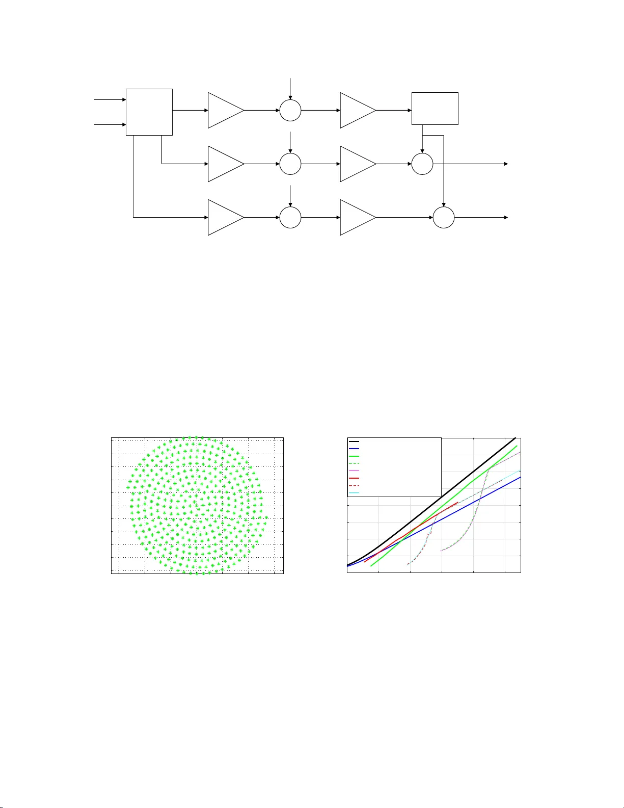
Shannon-K otel’nik o v Mappings for Analog Point-to-Point Communications P ˚ al Anders Floor , T or A. Ramstad, Abstract In this p aper a n appro ach to joint source-ch annel coding (JSCC) named Shannon- K otel’nikov mapping s (S-K m appings) is discussed. S-K mapping s are continuo us, or piecewise co n tinuous direct source-to- channel mapping s operating dir ectly on amplitude c ontinuo u s and discrete time sig n als. Such mapping s include se veral existing JSCC schemes as special cases. Many existing approache s to ana log- or hybrid discrete analog JSCC provide both excellent performan ce as well as robustness to variable noise lev el at low delay an d re lati vely low com plexity . Howe ver , a general th eory explainin g their perfor mance and beh aviour , as well as guid elines o n ho w to construct close to o ptimal mapp ings, do no t curren tly exist. T herefor e, such mapp ings a r e often based o n educated guesses inspir ed b y conﬁg urations that are known in advance to pr oduce good solution s thro ugh numerical optim iz a tio n metho ds. The objective of this pap er is to dev elop a theoretical fram ew ork f o r a n alysis of ana lo g- or hybrid discrete analo g S-K mapping s wh ich enab le s calculatio n o f distortion when apply in g them on point-to- point links, re veal more ab out their f undame n tal natu re, and p rovide g uidelines f or their co nstruction at low ( and arbitrar y) complexity an d dela y . Such guideline s will likely help constrain solutions to nu merical app roaches an d help explain why mach ine lea rning approach es ob tain th e solutions they do. The overall task is d ifﬁcult and we do not p rovide a co m plete framew ork at this stage: W e focus o n h igh SNR an d memoryless sources with an arbitrar y contin u ous un imodal density fun ction an d m emoryless Gau ssian channe ls. W e also p r ovide example mapping s b ased on surfaces which are cho sen based o n the provide d theor y . Index T erms Joint sourc e chann e l co ding, analo g mapping s, d istortion analysis, differential geometr y , OPT A. P . A. Fl oor is with t he Colour Laboratory , Department of Computer Science, Norwegian Uni versity of Science and T echnolog y (NTNU), Gjøvik, Norway (e-mail: paal.anders.ﬂoor@ntnu.no ). T . A. Ramstad is Prof. E meri t us at the Department of Electronic Systems, Norwegian Unive rsity of Science and T echnolog y (NTNU), Tron dheim, Norway (e-mail: tor .ramstad@ntnu.no). This work wa s supp orted by NTNU via the p roject CUB AN and the Research Counc il of Norway (NFR) via the project MELOD Y nr . 187857/S10. Parts of this paper have previously been presented at SP A WC 2006 [1], NORS IG 2006 [ 2] and ITW 2007 [ 3 ]. March 22, 2022 DRAFT 1 Shannon-K otel’nik o v Mappings for Analog Point-to-Point Communications I . I N T R O D U C T I O N Over the last decades more and m ore attentio n has been directed towar ds miniature de vices, for example in-body sensors and miniature electronic modules re placing ceratin neural net work function in the brain. For t his reason, and sev eral others, it has become important to study communication systems wit h low complexity and del ay wi t h the highest pos sible performance. Further , it is crucial to d eterm i ne performance l i mits of such schemes. In t his paper we in vestigate a general set of analo g or hybrid di screte-analog joint source- channel coding (JS CC) schem es named Shannon-K ot el’nikov mappings (S-K m appings). S-K mappings operate di rectly on analog information sources and are known to perform well at low complexity and delay [4], [5], [6], [7], [8], [9]. Shannons’ separation theor em or information t ransmission theore m (see e.g. [10, pp . 224- 227]) for commun ication of a single so u rce over a point-to-po i nt link states that s o urce coding and channel coding can be performed separately , with out any loss com p ared t o a joint techniq u e. T o prove that separation is o ptimal, arbitrary complexity and delay is assumed. W ith a constraint on com plexity and delay , separate source and channel coding (SSCC) does not necessarily resul t in the best possib l e performance, as so me e xamples illustrate: It was sho wn in [11], [12] that for an independent and identi cally distributed (i.i.d.) source and an additive white Gaussian noise (A WGN) channel, both of t he s ame b and w i dth, t h e in form ation theoretical bound 1 is achie ved by a simple linear sou rce-channel mapping operating on a symbo l -by-symbol basis. This resul t was generalized in [12], [13] to s p ecial com binations of correlated sources and channels with m em ory . Furthermore, it was shown in [14], that with an ideal feedback channel, the information theoretical bound is achieved when the channel-source bandwidth ratio is an integer . This was extended to simp l e sensor networks i n [15]. Ho wev er , with limited (or no) feedback, t h e asymptotic bounds cannot be obtain ed a t ﬁ nite complexity and delay when so urce 1 By information theor etical bound we refer to a bound deri ved with no restriction on complexity and delay . March 22, 2022 DRAFT 2 and channel are of different bandwidth or di mension, or in general, when t h e source and chann el are not probabilistically matched [16]. An open q u estion is what the best possi ble performance is for this ca se under complexity and delay constraints. Ef forts dealing wit h this issue are Kostina and V erd ´ u [17], [18] and M erhav [19], [20]. Se veral analog and s emi-analog JSCC schemes for the bandwidth mismatch case, operating at l ow and arbitrary com plexity and delay , hav e been suggested i n t he literature: The ana l og matching scheme in [21] is a structured semi-analog approach b u ilt on lat t ices that achiev es the information theoretical bo unds in the l i mit of inﬁnite compl exity and delay for any colored Gaussian s o urce transmitted on an y colored Gaussian channel. Howe ver , th e performance of analog matching scheme in the ﬁnite complexity and delay regime is, to our knowledge, unknown at present. Schemes that are kno wn t o perform well at lo w comple xity and delay are the hybri d digital-ana l og (HD A) schemes in [22], [23], [24], [4], [25], [26], certain analog mappi n gs like the Ar chimedes Spiral [27], [28], [29] and mappi ngs found by m achine learning [9]. The approach to JSCC st udied in this paper , namely S-K mappings, is insp ired by man y earlier works: First of all, Shannon suggested the use of conti n uous mapp i ngs through space curves as a wa y o f getting close to the inform ation theoretical bounds [30]. Sim ultaneously , K otel’nikov de veloped a theory for analyzing distortion o f certain amplit u de continuo u s and time discrete s ystems realized as parametric curves in N di mensions 2 in [31]. The efforts of Goblick [11], Berge r et al. [12] and V aishampayan [32], [33] are pioneering works on t his subject. The ef fort by Gastpar et. al. [16] is another important cont ri bution and Merha v ’ s ef forts [19], [20] provides insight into the underlying w orkings of such scheme through analysis based on statistical mechanics. Other important w orks includes th e deve lopment of power constrained channel opt imized vector quantizers (PCCO VQ) [32], [34], [35], the HD A schemes in [22], [23], [24], [4], the linear bloc k pul se amplitu d e modulati o n (BP AM) schem e in [36], [32] and the use of parametric curv es for bot h b andwidth expansion [33] and compression [ 27], [28]. Other recent eff orts dedicated to analog or semi-analog mappi ngs are found in [5], [37], [38], [39], [21], [40 ], [41], [8], [42]. Lately machine learning was applied to ﬁnd the o ptimal structure of such mappings [9]. These ef forts illustrate that such schemes perform well at lo w complexity and delay , som e providing excellent performance not matched by any other known scheme. 2 These are basically bandwidth (or dimension) exp anding systems with pulse position modulation as a special case. March 22, 2022 DRAFT 3 Besides Goblikc’ s [43], Gastpar’ s [16] and M erha v’ s approaches [19 ], [20], th ere are, as far as we know , no theory providing m eans t o analyze such mappings nor guideli ne for constructi on on a general basis. The obj ective of this paper is therefore to introduce a theoretical framework based on differ ential geometry , encompassing many analog and hybrid discrete-analog s chemes. This approach seeks to compl ement that of M erha v and Gastpar . The propo s ed theoretical framework facilitate calculation and analysis of t h e ove rall disto rtion in order t o re veal the fundamental nature o f S-K mappi ngs, as well as guidelines on their construction. The m ain reason for dev eloping a theory i s to gain knowledge on how to optimally const ruct such mapp i ngs in general, not h aving to rely on educated gu ess es, num erical optimization sensitive to i nitial condit ions, or machine learning approaches in whi ch little is k n own about why a certain resul t is p roduced. T reating nonlin ear m appings on a general basis is a difﬁc ult prob l em, and we do not present a complete theory at this point, rather int roduce a set of t ools providing insights on the cons t ruction of S-K mappi ngs. W e limit the study to m emoryless and independent analog sou rces drawn from an arbitrary uni modal densit y function. The sources are transmitted on m emoryless, ind epend ent Gaussian p o int-to-point channels, po s sibly with limited feedback providing channel s tate infor- mation. Generally , the mappin gs apply when t he c hannel-source dimension (or bandwidth) ratio is a positive rational num b er . Most of t he resul ts provided are proven under th e assum ption of high signal-to-nois e ratio (SNR). W e focus on low compl exity and delay but also consider ho w these mappings potentially perform by lettin g their dimensio n ality increase. That is, what gains may be obtained if we increase the mappings dim ensions i n order to code blo cks of samples. Finally , we provide particular examples on mappings chosen b ased on the provided theory . The paper is organized as follows: In Sec tion II t he probl em is formulated, the information theoretical lim i t OPT A is introduced, S-K m appings are deﬁned and key concepts from differential geometry are presented. In Section III a di stortion framework for S-K mappings b ased on concepts from differe ntial geom etry is developed and guidelines for their constructio n are g iv en. In Section IV asymptoti c analysis is considered and it is shown under which conditions S- K mappings may achieve optim ality for Gaussian sources. Section V provides examples on construction of S-K mappings us ing surf aces to illustrate the theory developed in preceding sections. In Section VI a discussion is giv en. March 22, 2022 DRAFT 4 I I . P RO B L E M F O R M U L A T I O N A N D P R E L I M I N A R I E S Assume a source x ∈ R M , drawn from a cont i nuous unimodal multiva riate prob abi lity density function (pdf) f x ( x ) , with i. i .d. components x i . x is mapp ed throu g h an S-K mapping (deﬁned i n Section II-B) to a ve ctor z ∈ R N which is transmitted ov er a memoryless channel with a verage power P , so that 1 / N P N i =1 E { z 2 i } ≤ P , and additive Gaussian noise n ∈ R N with joint pdf f n ( n ) with i.i.d. com ponents n i ∼ N (0 , σ 2 n ) . The channel out put ˆ z = z + n is mapped through an S-K m apping at the recei ver to reconstruct the source. As a measure of performance, the end-to-end m ean s q uared error per source sample between the input - and reconstructed vector , D t = (1 / M ) E {k x − ˆ x k 2 } , is consid ered and com pared t o the opt i mal performance theor etically atta i nable (OPT A) [12]. A. OPT A OPT A in the i.i.d. case is obtained by equati ng the rate-distort ion function for the rele va nt source with th e relev ant channel capacity . The equatio n is solved with respect to the sig n al-to- distortion ratio (SDR), which becomes a function of the channel signal-to-nois e ratio (SNR) [12]. For the case o f Gaussian sou rces and channels, OPT A is explicitly give n by σ 2 x D t =  1 + P σ 2 n  f c /f s =  1 + P σ 2 n  N/ M , (1) where σ 2 x is the source variance , σ 2 x /D t is the SDR and P / σ 2 n is the channel SNR. Assuming Nyquist samp l ing and an ideal Nyquist channel, the ratio between channel signalli ng rate f c , and source sampling rate f s , can be obtained by combini ng M source samples with N channel samples. That is, f c /f s ≈ N / M = r , where r is a positiv e rational number ( r ∈ Q + ), named dimension change factor . If r > 1 , the channels dimensi on is h i gher t h an that of the source and this can be utilized for noise reduction . If r ∈ [0 , 1) , the sou rce dimension, and hence the information, has t o be re duced i n a l ossy way before transm ission. W e denote the operation where a so u rce of dim ension M is mapped onto a channel of dimension N an M : N mapping. B. Shann o n -K otel’nikov mappings S-K mappings operate directly on ampl itude cont inuous, discrete time signals. Let S denote a general S-K mappin g and S a speciﬁc realization. W e h ave the following deﬁnition: March 22, 2022 DRAFT 5 Deﬁnition 1: Sha n non-K otel’ni ko v mapping An S-K mappi ng S is a continuous or pi ece wise conti nuous nonli near or linear mapping between R M (source space) and R N (channel space). T h ere are t h ree cases to con s ider: 1. Equal dimension M = N : S is a bijective 3 mapping. 2. Dimension expansion M < N : S ⊆ R N is a mapping that can be rea lized by a hyper surface described by the parametrization 4 S ( x ) = [ S 1 ( x ) , S 2 ( x ) , · · · , S N ( x )] , (2) where each source vector x should ha ve a unique representation S ( x ) ∈ S . S is th en an M dimensional (locally Eu clidean) manifol d embedded in R N . 3. Dimension reduction M > N : S ⊆ R M is a mapping th at can be realized by a hyper surface described by the parametrization S ( z ) = [ S 1 ( z ) , S 2 ( z ) , · · · , S M ( z )] , (3) where each channel vector z should hav e a unique representati o n S ( z ) ∈ S . S is t h en an N dimensional (locally Eu clidean) manifol d embedded in R M .  Case 1 is trivial for Gaussian i.i.d. so urces, i.e. OPT A is obtained by a linear m apping with MMSE decoding at the receiv er (often referred to as uncoded transmi s sion) [11]. This paper is concerned wi t h the case M 6 = N (case 2 and 3). Howe ver , the M = N case fall out as special cases for som e of the resul ts given. Piecewise continui t y is considered in order to include hy brid discrete-analog (HD A) schemes. C. Relevant concepts from di ffer ential geometry The theory of S-K m appings is based on concepts from differential geometry which m ay be unknown to some readers. A brief introduction to necessary concepts are given here with more details provided in Appendix A and [44] which is av ail able o nline. All concepts p resent ed are taken from Kreyszig’ s book [45]. W e u s e variables u ∈ R and u i ∈ R here to keep the discussion general, not s p eciﬁcally referring to source- or channel variables. 3 MMSE decoding is needed at low SNR in order to obtain optimality , effecti vely weaken ing this condition. 4 This is not a restriction, i.e. t he mapping does not need to be described by a parametrization. March 22, 2022 DRAFT 6 Consider a parametric curve ( 1 : N or M : 1 mappi ngs), C : S ( u ) = [ S 1 ( u ) , S 2 ( u ) , · · · , S n ( u )] ∈ R n . In th e following we denote the deriv ativ es wi t h respect to (w .r .t) to a g eneral parameter , u , as S ′ , S ′′ etc. In the sp ecial case of the parameter being the ar ch lengt h , we denot e the deriv ativ es ˙ S , ¨ S etc. T h at is, wh en we parameterize the curve via ℓ ( u ) = Z u u 0 √ S ′ · S ′ d u = Z u u 0 k S ′ k d u. (4) Then k ˙ S k = k t k = 1 , ∀ u , with t the curves tangent vector(s) (See Ap p endix A-A). For a curve, S ( u ) , one can deﬁne curvatur e w .r .t. arch length at u 0 as κ 0 = k ¨ S ( u 0 ) k [45, p. 34]. Consider arc l eng t h parametrization with an ampliﬁcation α , w h ich we name scaled ar c length pa rametrization . Then k S ′ ( u 0 ) k = α k ˙ S ( u 0 ) k = α , ∀ u 0 , and κ ( u 0 ) = k S ′′ 0 ( u 0 ) k / k S ′ 0 k 2 according to Appendix A-A. Th e torsion [45, p. 3 7-40] i s deﬁned as τ ( x ) =   ˙ S ¨ S ... S   / k ¨ S k 2 . When τ = 0 , ∀ x , we have a plane curve. Whenever τ 6 = 0 , th e curve will t wist up into space ( R n ). For surf aces, S , with parametric representati on as (2), (3), we denote partial d eri vati ves as S α = ∂ S ∂ u α , S αβ = ∂ 2 S ∂ u α ∂ u β . (5) The use of subscript s and superscripts h ere relates to Eins t ein’ s summation conve ntion which is described in A p pendix A-B. The curvature of a surface S depend s on the choice of coor dinate curves on S : A curve, C , on surface S : S ( u 1 , u 2 ) is represented by the parametrization C : u 1 = u 1 ( t ) , u 2 = u 2 ( t ) , wh ich is ∈ C 1 (the set of differentiable functions), where t ∈ R . The coordinate curves, u 1 = constant and u 2 = constant, correspon d s t o parallel curves in the u 1 , u 2 -plane. On e must always choos e allowable coor dinates whi ch conditions are provided in [44, p.2]. The normal curvatu re , κ n , of S at point P is given by κ n = b αβ d u α d u β /g αβ d u α d u β (see Appendix A-B3, Eqn. (70)) , wher e g ij = S i · S j are the compon ent s of the me tric tens o r , or ﬁrst fundamental form (FFF) of S , and b αβ = S αβ · n are com ponents of the s econd fundamental form (SFF) of S , with n , the u nit normal to S at P (see Appendi x A-B2 for d et ai l s). A special case of particul ar interest is the extremal values of κ n , named lines of curvatu re (LoC). If one chooses LoC as coordinate curves then the curv ature of S in those directions, the principal curvatur e , are giv en by κ i = b ii /g ii , ∀ i (see Appendix A-B3 for details). For general coordinate curves, κ i are the roots of (72) in Appendix A-B. The normal curvature κ n for any March 22, 2022 DRAFT 7 (tangent) direction can be represented in terms of κ 1 and κ 2 according to t heor em of Euler [45, p. 132] (see also [44]) as κ n = κ 1 cos 2 α + κ 2 sin 2 α , with α the angl e bet ween an arbit rary direction at P and the direction corresponding to κ 1 . I I I . D I S T O R T I O N A N A L Y S I S F O R S - K M A P P I N G S In this section we quantify d istortion for S-K mappin g s. A. Dimensi o n e xpanding S-K ma p pings. In this section K otel’nikovs t heory from [31, pp.62-99] on 1 : N mappings is generalized to include vector sources, enabling analysis of more general m appings. The results presented in this section are extensions of [1]. Fig. 1 depicts the bl o ck diagram for a dim ens ion expanding S-K communication system. Consider source vector x ∈ D ⊆ R M , with do main D . The source is represented by a a sign a l ⊆ ∈ x x ˆ ∈ = ) ( x S z + ⊂ ML detector z ˆ n ) ( ⋅ S Fig. 1. Dimension expanding ( M < N ) communication system for S- K mappings. hyper surface in the channel space x 7→ S ( x ) ∈ S ⊂ R N , (see Deﬁnition 10). Applying a speciﬁc realization of S , S , t h e likelihood function o f t he receiv ed signal ˆ S = S ( x ) + n is f ˆ S | x ( ˆ S | x ) =  1 2 π σ 2 n  N/ 2 e − k ˆ S − S ( x ) k 2 2 σ 2 n , (6) The maxim um likelihood (ML) estimate is then deﬁned as [46] 5 ˆ x = max x ∈ R M f ˆ S | ˆ x ( ˆ S | x ) , (7) and is m axi mized by t he vector x that minim izes k ˆ S − S ( x ) k . I.e., the M L estim ate of x corresponds to the point on S clos est to the recei ved vector in Euclidean dist ance. 5 Ideally MMSE estimation should be considered but is difﬁcult to deal with analytically for such mappings. T his will result in a loss at lo w SNR . See for example [41]. March 22, 2022 DRAFT 8 Ideally on e could formulate t he exact distortio n for any such scheme once a speciﬁc represen- tation S is chosen. Howe ver , this i s incon venient when it comes to analysis of the behavior of such m appings as it is usually very hard, if at all possib le, to ﬁnd closed form so lutions. For this reason we use an approach su ggested b y Kotel’niko v in [31, pp.62-99]. Kotel’niko v reasoned that there a re tw o main contributions to the to tal dis tortion usi n g such mappings: low intensity noise and strong nois e . Low intensity no i se is when the error in the reconstruction at the decoder v aries gradually with the magnitude o f t he noise samples. Distortion due to lo w i ntensity noise can be analyzed with out reference to a speciﬁc S when t he noise can be consi dered weak . Th e resultin g distortion is named weak noise di stortion , denoted b y ¯ ε 2 w n , as deﬁned i n section III-A1. Strong noise is known as anoma lous err ors i n the literature, and results from a thr eshold effect 6 [30]. The resulti ng distortion is named anomalous dist ortion and denoted by ¯ ε 2 an . 1) W eak noi s e di stortion: T o analyze non-linear m appings w i thout re ference to a s peciﬁc structure the concepts introduced in Section II-C and the T ayl or expansion apply . W e begin by quantifying weak noise distorti on : Let S lin ( x ) denote 1st order T aylor approximation of S ( x ) at x 0 S lin ( x ) = S ( x 0 ) + J ( x 0 )( x − x 0 ) , (8) where J ( x 0 ) denotes the J acobian (see Appendix A-B) of S ev aluated at x 0 . Fig. 2(a) shows how the ML estimate is computed by the approximation in (8) for the 2 : 3 case. W e have the following proposition providing the exact distortion under li near approximatio n: Pr o p osition 1: Mi n imum weak noise distort ion For an y continuous i.i.d. s o urce x ∈ R M with unimodal pdf f x ( x ) communicated on an i.i.d. Gaussian channel of dimension N using a continuous dim ension expanding S-K mapping S where S i ∈ C r ( R M ) , r ≥ 1 , i = 1 , .., N , the min i mum dist ortion under th e linear approximati on in (8) is given by ¯ ε 2 w n = σ 2 n M Z Z · · · Z D M X i =1 1 g ii ( x ) f x ( x ) d x , (9) obtained when the metric tensor (or FF F) G of S (Appendix A-B) is diagonal with entries g ii = k ∂ S ( x ) / ∂ x i k 2 . I.e., the squared norm of t he tangent vector along t h e i’th coordinate curve. Pr o o f: See Appendix B-A1.  6 A thorough treatment of threshold effects, going beyond what we present here, is gi ven in [20], [47] March 22, 2022 DRAFT 9 The name weak noise distortion is due to Deﬁnition 2 given later in this section. Eqn. (9) states that weak nois e distortio n becomes s m aller by increasing the g ii ’ s. This is equivalent to making tangent vec tors at an y given point of S longer , and is obtained by stretching S l i ke a rubber -sheet. Bendin g , o r cutt ing, of the signal hyper surface does not re duce weak noise distortion. The concept is illustrated i n Fig. 2(b) for t he 1 : N case when S is a curve. Stretching of the 0 Noise Detected vector Error Received vector Transmitted vector (a) Source Stretched source x 2 x 1 noise noise x 1 x 2 (b) Fig. 2. Dimension exp anding S-K mappings. 2(a) ML estimate approximation for a 2 : 3 map ping under the weak noise regime. 2(b) Kotel’nik ovs concept of analog error reduction for 1 : N mappings. curve makes source vectors appear longer com pared to a given noi se vector , or equiv alently , the more t he source is stretched at the t ransmitter trou gh S th e more th e nois e wil l be attenuated at the rece iver , resulting in sm aller distortion. This result by itself implies that the s ource space should be stretched ind eﬁnitely . Howe ver , as will be seen in Section III-A2, under a channel power constraint, this cannot be done wit h out introducing large anomalous errors. Remark 1: Proposit i on 1 is e xtendable to piecewise continuous mappings s ince one can inte- grate over each surface element, then sum all the contributions afterwards (see example in [22]). The following corollary is a special case o f Proposition 1: Cor oll ary 1: Shape pr eserving mapping March 22, 2022 DRAFT 10 When S has a diagonal m et ri c G with g ii ( x ) = g j j ( x ) = α, ∀ x , i, j , and with α a constant, then ¯ ε 2 w n = σ 2 n α 2 . (10) That is, all source vectors are equally scaled when mapped through S and t he noise wi ll affe ct all values of x equally . Pr o o f: Insert g ii ( x ) = g j j ( x ) = α in (9).  A shape preserving mapping can b e seen as an ampl iﬁcation factor α from source to channel. Although a shape preserving mappin g leads to sim p le analysis, i t s not necessarily opti m al in general. A resul t obtain ed in [48, 294 -2 9 7 ] using variational calculus can b e used for 1 : N mappings to ﬁnd the opt imal g 11 ( x ) for a given source pdf. In order to determine the error m ade in the dis t ortion estimate under linear approximat i on, we need to consider 2 n d order T aylor expansion. W e have the following proposition: Pr o p osition 2: W eak noise err or under 2nd or der T aylor appr o ximation Under 2nd order T ayl or approximation, the special case of 1 : N mappings (curv es) has an error in the absence of anom alies given by ε 2 w n ≈ σ 2 n k S ′ 0 k 2  1 + 1 4 σ 2 n k S ′′ 0 k 2 k S ′ 0 k 4  = σ 2 n k S ′ 0 k 2  1 + 1 4 σ 2 n κ 2 ( x 0 )  , (11) valid for any S-K mapping S ( x ) ∈ C n , n ≥ 2 . T h e last equality is t rue under scaled arc lengt h parametrization. Further , for any dimension expanding S-K mapping as deﬁned in Deﬁnition 10, with LoC coo rdinate curves, the error is given by ε 2 w n ( x 0 ) ≈ σ 2 n M M X i =1  1 g ii ( x 0 )  1 + σ 2 n 4 b 2 ii ( x 0 ) g 2 ii ( x 0 )  = σ 2 n M M X i =1  1 g ii ( x 0 )  1 + σ 2 n 4 κ 2 i ( x 0 )  . (12) Here, κ i = b ii /g ii is the curv ature along coordinate curv e i with b ii the diagonal components of the second f undamental form (SFF) as described in Appendix A-B . Pr o o f: See Appendix B-A2.  Remark 2: W e o nly treat 2nd order T aylor approxi m ation here to simplify analys is. It will be seen in Section I II-B that higher order terms are e ven less inﬂuenti al as σ n is raised to a power twice that of the order , which at hi g h SNR ( σ n << 1 ) l eads to a negligible contribution. Note t hat i n the absence of anomalies, one can characterize dis tortion for S-K mappings in general without choo s ing a speciﬁc S in advance, as i t is expressed solely w .r . t . FFF and SFF components. This m akes it easier to ev aluate the distortio n analytically for such mappings. March 22, 2022 DRAFT 11 From (12 ) alone a li near mapp i ng seems con venient as κ i = 0 , ∀ i . Howe ver , at h igh SNR linear mappings perform poorly , and with (12) in mind, one would s eek nonlinear mappings with the sm allest possible κ i ( x ) . Therefore the weak noise regime, as deﬁned next, is a good approximation for any r easonably chosen mapping at high SNR. Deﬁnition 2: W eak noise r e gime (dimension expansion) Let x 0 denote the transm itted vector and S ( x 0 ) its representation in t he channel s pace. W e say that we are in th e weak noise re gime whenever the 2nd order term in (12) (the term containi ng κ i ), is negligible com pared t o the 1st order term. That is, (8) is a close approxi mation to S and the weak noise dist ortion i n (9) provides an accurate approxi mation to the actual distortion in the absence of anomalies.  Example 1: When is Deﬁnition 2 satisﬁed? There are at leats three cases: i) SNR → ∞ ( σ n → 0 ): The linear approxi m ation in (8) is exact as S is lo cally Euclidean. ii) S i s linear or HD A: Then κ i = 0 , ∀ i . A linear mapping is opt imal when SNR → 0 [36], [49]. HD A systems are composed of piecewise line- or (hyper) plane patches. iii) Small maximal principal curv ature κ max : The smaller κ max is, the larger σ n can be before (9) becomes inaccurate. This is also inline wit h solution s resulti n g from numerical optimization algorithms, which tend to bend less and less the lower the SNR is [35], [50]. 2) A nomalous dis t ortion: W ith a channel power c onstraint, S m ust be cons trained to lie within s ome N − 1 sphere 7 , S N − 1 . In order to make weak noise d i stortion small, the rele vant hyper surf ace must ﬁrst be stretched, then bent and twisted to ”ﬁt” within this sphere. Fig. 3(b) illustrates how this ca n be done in the 1 : 2 case. T ake a decompo sition of the noise n into a tangential component to the sign al curve n w n = n || , a nd a normal com ponent n an = n ⊥ as d epi cted in Fig. 3(a). n w n contributes to weak noise, whilst n an contributes to ano m a lous err ors , which are lar ge errors occurring whene ver k n an k cross es a certain threshol d. Then the transmitted vector S ( x 0 ) representing x 0 , will be detected as t he vector S ( x er r ) on another fold of the curve. This happ ens if the distance, ∆ , between the spiral arms is chosen too small w .r .t. σ n . Althoug h S ( x er r ) is not far away from S ( x 0 ) in the channel space, the value i t re presents, x er r , is f ar a way from x 0 in so u rce space, leading to lar ge reconstruction errors. The occurrence 7 The deﬁniti on of an N -sphere is S N = { y ∈ R N +1 | d ( y , 0) = constant } [51, p.7], where d is t he distance f r om any point y on S N to t he origin of R N +1 . E. g. the spher e embedded in R 3 is denoted S 2 , the “2-sphere”. March 22, 2022 DRAFT 12 0 0 z 1 z 2 s(d) s(−d) Constrained region Linear mapping Nonlinear mapping ∆ n an n wn (a) 0 0 z 1 z 2 s(x 0 ) s(x err ) n (b) Fig. 3. E xample of 1 : 2 S-K mappings ( ± d denote t he boundary of D ). 3(a) Linear and nonlinear mappings (negativ e source v alues represented by dashed curve). 3(b) As the spiral arms gets close, noise may take the transmitted vec tor S ( x 0 ) closer to another fold of the curve leading to large decoding errors. of anomalous errors d epend s on σ n , and t he min i mum distance ∆ min between folds of S as well as its curvature. For anomalous errors to occur with small probabi lity , ∆ min should be chos en as lar ge as possi ble. There is t hus a tradeof f between reducing weak noise distortion (where ∆ min should be as sm al l as possible) and anomalous disto rt i on. The exception is at l ow SNR where linear mappings may do just as well [36], [49]. In this case anomalou s errors do n o t occur , and we w i ll always be in the weak n o i se regime of Deﬁnition 2 as κ i = 0 , ∀ i in (86) (see Fig. 3(a) ). T o quantify anomalous distort ion it is con venient to consider canal surfaces [45, pp. 266-268]. W e b egin wit h curves ( 1 : N m appings). Deﬁnition 3: Canal surface A canal surface is the en velope , E , to the family , F , of cong ruent spheres (or N − 1 hyper-spheres S N − 1 ), and is the set of all characteristics to F , deﬁned by [45, p. 263 ] S c ( z i , x ) = 0 , ∂ S c ( z i , x ) ∂ x = 0 i = 1 , · · · , N , (13) where S c = 0 deﬁnes a s u rface in R 3 (or hypersurface in R N ). The characteristic is a curv e in R 3 (or a hypersurface o f dimension N − 2 in R N ). The characteristic points of the canal surface March 22, 2022 DRAFT 13 are the i ntersection of t he characteristics given by [45, p. 266 ] S c ( z i , x ) = 0 , ∂ S c ( z i , x ) ∂ x = 0 , ∂ 2 S c ( z i , x ) ∂ x 2 = 0 , i = 1 , · · · , N . (14)  An important special case is the family , F , of spheres with constant radiu s r and center on a curve C : y ( x ) , which can be re presented as S c ( z , x ) = ( z − y ( x )) · ( z − y ( x )) − r 2 = 0 . In this case the characteristics of F are circles and the characteristic points are points of intersection of th ese circles. This concept can be directly applied to 1 : N S-K m appings in Gaussian noise by setting y = S ( x ) , with z the channel coor dinates and x the s ource values. The extension to M : N mappings is straight forward: The canal hypersurface o f an M- dimensional S embedded in R N is the en velope of the congruent hyper -spheres S N − M − 1 . W e refer to a canal hypersurface simp ly as “canal surface” in the following. Canal surfaces are important for S-K mappi ngs as they under certain con d itions can guarantee low probability for anomalous errors. Lemma 1: Consi der M : N dimension expanding S . Let ρ min = 1 /κ max , with κ max the m axi mal principal curvature of S , and r the radius of the hyper-sphere S N − M − 1 . F urther , l et ∆ min be the minimum distance between any fold of S for any x : Then the corresponding canal surface, the en velope of S N − M − 1 , will not int ersect itself at any point. That i s , the canal surface wi ll hav e no characteristic poi nts ⇐ ⇒ i) ∆ min > 2 r and i i) ρ min > r for all poi n ts of S . Pr o o f: See Appendix B-A3.  Remark 3: Note that con dition ii) i s incorporated into conditio n i). The reason we explicitly state ii) is to constrain the curvature of S so th at it can be removed from the analysis l at er . Example 2: W e give an example on a 1 : 3 mapping. Fig. 4 depicts a canal surface surround ing a curve in channel sp ace R 3 . The radius of the canal surface is lin ked to the noise vector n an = n ⊥ . Bending of the tube can i ncrease t he prob ability for anomalou s errors, i mplying th at s t raight lines have the lowest probability for such errors. F rom this perspective, non-linear m appings seem to be sub-op t imal. Ho wever , acc ording to Lemma 1, one can circumvent t h is if t he radius of curvature of S is s mall enoug h. The signiﬁcant p robability mass 8 of the normali zed noi se vector n an is located wi t hin a circle of radius ρ n = p 2 b 2 n σ 2 n / 3 , wi th b n related to the variance 8 signiﬁcant pr obability mass refers to all e vents except those with very low probability . E.g., li ke the “ 4 σ loading” used in [52, pp. 124-125] when constructing scalar quantizers. March 22, 2022 DRAFT 14 Cross sections Tube Bent tube ) ( 0 x S ) ( 0 x S an n wn n an n an n Fig. 4. Canal Surfaces: T op ﬁgure: Li near signal curve L × S 1 . Bottom ﬁgure: nonlinear signal curve S × S 1 . of n an (typically b n > 4 incorporates abo u t 99 . 99% of the probability mass when the dimens ion of n an is sm all). Therefore, if i) is s atisﬁed, and if ρ s > r = ρ n ≥ r N − 1 N b n σ 2 n , (15) then no characteristic points exists, and t he canal s urface will not intersect itself. W e provide a deﬁnition of anomalous distortion valid in the vicinity of the optimal operational SNR. That is, we onl y consider jum ps to the nearest point on ano t her fold, S ( x er r ) , from a given transmitted poi nt, S ( x 0 ) (j umps across sev eral folds may happen as σ n grows, b ut t his is far from opt i mal). Fig. 3 shows the terminol ogy used in t h e following deﬁnition. Deﬁnition 4: Ano m a l ous distortion Let x 0 denote the transmit ted v ector and S ( x 0 ) its representation in the channel space. Let n an denote the K ( ≤ N ) dimension al com ponent of a decomposi t ion of the noise vector n that poin t s in the direction of t he clos est point S ( x er r ) on any ot her fold of S from S ( x 0 ) (as seen i n Fig. 3(a)). x er r ( x 0 ) d enotes the reconstructed vector i n the case o f th i s anomaly . Let ∆ min ( x 0 ) deno te th e Euclidean d istance bet w een S ( x 0 ) and S ( x er r ) . Further , let ρ an = k n an k with f ρ an ( ρ an ) its pdf. The probabi lity that x 0 is detected as x er r is then P an ( x 0 ) = Z ∞ ∆ min ( x 0 ) / 2 f ρ an ( ρ an ) d ρ an . (16) The anomalo u s distortion close t o the opt imal operational SNR is then deﬁned as ¯ ε 2 an = E x  P an ( x ) k x − x er r ( x ) k 2  . (17)  March 22, 2022 DRAFT 15 B. M : N Dimension Reducing S-K mappings . Results presented in this section are extensions of [2]. Fig. 5 shows a blo ck diagram for the dimension reducing communication s ystem under consideration. As d eﬁned in Sec tion II-B, a n ⊆ ∈ x ) ˆ ( ˆ z S x = z ˆ + ) ( ⋅ S ∈ ) ˆ ( z S ∈ = ) ( x p z ) ( ⋅ p   Fig. 5. Dimension reducing ( M > N ) communication system for S -K mappings. dimension reducing S-K mapping s S is an N dim ensional subset of the source space R M that can be realized by a hyper surf ace S as in (3), parameterized by the channel signal z . In this sense, the S-K mappin g is a representati o n of the channel in the source space. T o reduce the d imension of a source under a channel power constraint, some of its informati on content will be lost. The source vectors x are approximated by their projection onto S , an operation denoted q ( x ) ∈ S ⊂ R M . The dim ension is subsequent ly changed from M t o N by a lossless operator d r : S → D c ⊆ R N , where D c is the domain of th e channel signal determined by the channel power constraint. The total operation is named pr ojection o p eration , and denoted p = d r ◦ q : x ∈ R M 7→ p ( x ) ∈ D c ⊆ R N . The vector z = p ( x ) i s transmitted over an A WGN channel with no ise n ∈ R N . Channel n o ise will lead to displ acements of the projected source vector along S . W ith a continuous S , th e dist ortion d ue t o channel no i se will be gradual l y increasing with σ 2 n , i.e. no anomalous errors wi l l occur . Howe ver , anomalo u s errors may occur if S is piecewise con tinuous (like HD A schemes). Considering ML detection, the reconst ructed vector is ˆ x = S ( ˆ z ) . The concept is illustrated for a 2 : 1 mappi n g in Fig. 6(b). There are two m ai n contributions to the total distort i on for contin uous S : approx imatio n distortio n from the lossy projection operation, and c hannel distortion resulting from channel noise mapped th rou gh S at the receiver . 1) Chan n el distortion: The recei ved vector ˆ z = z + n is mapped through S to reconstruct x . When noise is s u f ﬁciently small, distortion can be modelled by considering the tang ent space of S . That is, one can consider the linear approxim ation S lin ( z 0 ) of S ( z ) at z 0 , S lin ( z 0 + n ) = S ( z 0 ) + J ( z 0 ) n . (18) March 22, 2022 DRAFT 16 0 0 x 1 x 2 ∆ (a) x 1 x 2 x 0 Decision spiral ρ MN = ∆ /2 Tangent line Weak channel error x 0 ^ p(x 0 ) Large channel error Approximation error (b) Fig. 6. Dimension reducing S-K mapping in the 2 : 1 case. 6(a) Covering of source space w i th parametric curve. The dashed lines represent ne gativ e channel v alues. Green dots are source v ectors drawn from a 2D Gau ssian distribution. 6(b) Local behav ior . T he spiral segments are close to osculating circles. The following proposition give s the exact dis t ortion under linear approxi mation: Pr o p osition 3: Mi n imum W eak Channel Distort ion For any continuous i.i.d. Gaussian channel o f dimensio n N and any dimens i on reducing S-K mapping S where S i ∈ C r ( R M ) , r ≥ 1 , i = 1 , ..., M , the distortion due t o channel noise under the lin ear approximation in (18) is given by ¯ ε 2 chw = σ 2 n M Z Z · · · Z D c N X i =1 g ii ( z ) f z ( z ) d z , (19) where f z ( z ) is the channel pdf, and g ii the diagon al components of t he metric tens o r of S . Pr o o f: See App endix B-B1.  The name weak channel distortion is due t o Deﬁnition 5 given belo w . Proposition 3 states that weak channel di s tortion increases in magnitu de when S is stretched as the g ii ’ s increases. T o keep the channel d i stortion small, S should be stretched mi nimally 9 . The following corollary is a special case o f Proposition 3: 9 The opposite is sough t in the dimension expansion c ase as an increase of g ii leads to larger attenuation of noise at the recei ver side, whereas in the dimension r eduction case, increase of g ii will amplify the noise at the receiv er . March 22, 2022 DRAFT 17 Cor oll ary 2: Shape pr eserving mapping When S has a d iagonal metric with g ii ( z ) = g j j ( z ) = α, ∀ z , i, j , and α constant, then ¯ ε 2 ch = N σ 2 n M α 2 . (20) I.e. all channel vectors are equally scaled when m app ed throu g h S , and thus noise wi ll af fect all source vectors x equally . Pr o o f: Insert g ii ( z ) = g j j ( z ) = α in (19).  Under Corollary 2, S can be seen as an ampliﬁcation α from channel to source at the receiv er . As the channel noise becomes larger , (19) becomes inaccurate as illustrated in Fig. 6(b). T o determine the error under li near approximati o n, we consider 2nd order T aylor expansion: Pr o p osition 4: Er r or under 2nd or der T aylor appr oximation (dimension r eduction) Under 2n d order T aylo r approximatio n , in t h e special case of M : 1 mappings, the error due to channel nois e is given by ε 2 ch ( x 0 ) = σ 2 n k S ′ 0 k 2 + 3 σ 4 n 4 k S ′′ 0 k 2 k S ′ 0 k 4 = k S ′ 0 k 2 σ 2 n + 3 σ 4 n κ 2 ( x 0 ) 4 , (21) valid for any S-K mapping S ( x ) ∈ C n , n ≥ 2 . T h e last equality is t rue under scaled arc lengt h parametrization. Further , for any dimension reducing S-K mapp i ng as deﬁned in Deﬁniti on 10, with LoC coo rdinate curves, the error is given by ε 2 ch ( x 0 ) ≈ σ 2 n M N X i =1  g ii ( z 0 ) + 3 σ 2 n 4 κ 2 i ( z 0 )  = σ 2 n M N X i =1  g ii ( z 0 ) + 3 σ 2 n 4 b 2 ii ( z 0 ) g 2 ii ( z 0 ) )  . (22) Pr o o f: See App endix B-B2.  Comparing with d i mension e xpansion in Proposit i on 2 we see that di stortion is scaled by the components of the SFF (or curvature) in a similar manner . The scaling w .r .t . g ii is di fferent howe ver , corresponding to th e resul ts in (9) and (19). Remark 4: From the proof o f Proposition 4, Appendix B-B2, Eq . (93), we have ε 2 ch ( x 0 ) = σ 2 n k ˙ S ( x 0 ) k 2 + 3 σ 4 n 4 k ¨ S ( x 0 ) k 2 + 5 σ 6 n 12 k ... S ( x 0 ) k 2 = σ 2 n + 3 4 κ 2 0 σ 4 n + 5 12 κ 2 0 τ 2 0 σ 6 n , (23) for the channel error u nder 3 rd order T aylor expansion. The last equality is a canonical r epr esen- tation [45, p.48], valid for any curve S ∈ C 3 , r ≥ 3 . This shows that hi g her o rder t erm s become smaller as σ n decreases, at least for curves with smal l κ 0 and τ 0 . Referring to Section III-A , this is the reason why we did not cons i der T ayl or expansion beyond 2nd order there. March 22, 2022 DRAFT 18 Deﬁnition 5: W eak noise r e gime (dimension r eduction) Let z 0 denote t he transmitt ed vector and S ( z 0 ) it s representation i n the source space. W e are i n the weak noise r e g i me whenever the second (or higher) order t erm in (22), i.e., the terms containing κ i , is negligible compared to the 1st order term. Th at is, (18) is a close approximati on to S and the weak channel distortion in (19) provides an accurate approximatio n to the actual di stortion due t o channel nois e.  Remark 5: Generally the error i n the M L-estimate increases with κ max (and τ ). Howe ver , for continuous mappings, κ max (and τ ) n eed t o be non-zero in order to cover th e s o urces space and thereby keep the approx i mation distortion lo w . One sho uld therefore c hoose a mapping that ﬁlls the sou rce space with the small est possi b le κ (and τ ). Alternati vely , one may choose HD A s ystems consisting of parallel lines or planes where κ i = 0 , at the expense of introducing anomalous err ors. Therefore the weak noise r egime is a good approxim ation for any reasonably chosen mapp i ngs at high SNR. 2) A ppr o ximation distorti on: Approx imation dis tortion results fr om the lossy operation p . Its magnit ude depends on the a verage distance source vectors have to S . In order to make the approximation d istortion as small as pos sible, S sh ould cover the source space so t hat ever y x is as close to it as poss i ble. Covering of the s ource s p ace is obtained by st retching, bending a nd twisting the transformed channel space S inside th e subset of the source s p ace with signiﬁcant probability mass (an example for t he 2 : 1 case is p rovided in Fig. 6(a) ). This i s in con ﬂict with the requirement of reducing channel d i stortion in which the s t retching of S should be minimi zed. There is thus a tradeof f between th e two distortio n contributions. Since approxim ation distortion is structure dependent, one cannot ﬁnd a closed form expression for it i n general. Ho we ver , one can ﬁnd a general expression v alid for certain simple mappi ng structures that becomes exact as the dimension of t he mappin g becomes large. Deﬁnition 6: Uni f orm S-K mappi ng For an S-K mapping where at each point , S ( z 0 ) , ∀ z 0 ∈ D c , t h ere is a ﬁxed dis t ance ∆ to the nearest point on a nother fold of S , is named uniform S -K mapping . The maximal approxim ation error from x to S will then be ∆ / 2 for any x to any point of S .  Remark 6: Note that for a uniform mappi ng, any vector being approx i mated to any poi nt of S will be conﬁned within a Canal Surface as deﬁned in Section III-A2, Deﬁnition 3. The 2 : 1 S-K mapping shown in Fig. 6(a) is a uni form mapping (except close to the origin). March 22, 2022 DRAFT 19 For un i form S-K mappings, a simi lar di stortion lower bound as t hat deri ved for vector quantizers in [53] can be found for small ∆ , i.e., a spher e bound [54]. W e ha ve the follo wing proposi tion: Pr o p osition 5: Sp her e bound for appr oximation distortion For a un iform S-K mapping with distance ∆ between closest points on neighboring folds , the approximation dist o rt ion is bounded by ¯ ε 2 q ≥ M − N 4 M ( M − N + 2) ∆ 2 . (24) As this is a sphere bound, equality is achiev ed in the limit when M , N → ∞ [54], with N / M = r a constant, when ∆ i s sufﬁciently small. Pr o o f: See App endix B-B3.  Remark 7: Note that the bound in (24) is e xact in some low-dimensional cases. For e xample when M = 2 , N = 1 u sing the Archimedes s p iral, as this case is equiva lent to a scalar qu ant izer . I V . A S Y M P TO T I C A NA L Y S I S F O R S - K M A P P I N G S W e inv estigate how S-K mappings p erform as the dimensionali t y 10 (or bl oc k-length ) of t he mappings increases. Th at is, can S-K mapping s achie ve OPT A as M , N → ∞ in general? A. Asymptot ic analysis for di mension e xpanding S -K mappings. W e det erm i ne under which conditions dim ension expanding S-K m app i ngs may achieve OPT A for ∀ r ∈ Q [1 , ∞ ) in the limit M , N → ∞ . W e only treat the case of Gaussian sources and channels. The resul ts presented are extensions of [3]. As proving t he existence of hyper su rface s s at i sfying a distortion criterion is hard, if at all possible, we use a geometrical ar gument and consider how l ar ge volume the transformed source will occupy in the channel space, a generalization of results presented in [55, pp.666-674]. W e start with a propositi on concerning anomalou s errors in t he asymptotic case M , N → ∞ : Pr o p osition 6: As ymptotic anomalo us distortion Let the n o i se be norm al i zed with the channel dimension N , ˜ n = n / √ N , and let ∆ min denote the smallest distance to the closest point, S ( x er r ) , on any other fold o f S for any transmitted vector S ( x 0 ) . Furthermore, with n an the K ( ≤ N ) dim ensional component of n poin t ing in the direction of S ( x er r ) from S ( x 0 ) . Then ¯ ε 2 an → 0 as K, N → ∞ if ∆ min > 2 p K/ N σ n . 10 I.e., letting M , N increase while r = N / M ∈ Q + is kept constant. March 22, 2022 DRAFT 20 Pr o o f: First consi der no rmalized Gaussi an noise vectors ˜ n . By deﬁnition, these vectors ha ve mean length σ n . It is shown in [55, pp. 3 24-325] t hat the variance of k ˜ n k decreases as N increases and th at lim N →∞ k ˜ n k = σ n with probabil ity one. For n an , a K ( < N ) dimensional subset of ˜ n , we get k n an k = p K/ N σ n with probabili ty one.  Remark 8: Proposit i on 6 is equiv alent to ha v ing no characteristic points for the canal surface as stated in Lemm a 1. I.e., 1 /κ max ≥ ρ n ≥ p b 2 n σ 2 n ( N − M ) / N , with K = N − M , where b n → 1 as M , N → ∞ . Proposition 6 is the ke y to imp rove performance b y increasing mapping dimens ionality: Consider Deﬁnitio n 4. The di s tribution o f ρ = k ˜ n k , ˜ n ∈ R N , is g iven by [56 , p. 237 ] f ρ ( ρ ) = 2( N 2 ) N 2 ρ N − 1 Γ( N 2 ) σ N n e − N 2 ρ 2 σ 2 n , N ≥ 1 , (25) where Γ( · ) is the Gamma functi on [57]. Fig. 7(a) shows (25) for selected values of N . Note 0 0.05 0.1 0.15 0.2 0.25 0.3 0.35 0 2 4 6 8 10 12 14 16 18 ρ f ρ N=1 N=2 N=8 (a) −2.5 −2 −1.5 −1 −0.5 0 0.5 1 1.5 2 2.5 3 −2.5 −2 −1.5 −1 −0.5 0 0.5 1 1.5 2 2.5 Constrained region Intersected 2:4 scheme 1:2 scheme ∆ 2:4 ∆ 1:2 (b) Fig. 7. 7(a) The pdf of ρ = k ˜ n k when σ n = 0 . 1 . 7(b) Performance i mprov ement by i ncreasing mapping dimensionality: The green dashed cu rve ill ustrates an intersected surface. As ∆ 2:4 < ∆ 1:2 for the same anomalous error probability , the 2 : 4 mapping may be stretched a bit further . T his increases the g ii ’ s and so ¯ ε 2 wn is reduced. that t he probability mass of ρ becomes more l o cated around σ n as N increases. Considering this ef fect w .r .t. S -K mappings , a gain can be ob tained when i ncreasing dimensionality as ∆ min can be reduced: Consider r = 2 , which can be accompl ished by both 1 : 2 and 2 : 4 mapping s . T ake a March 22, 2022 DRAFT 21 2 : 4 mapping with di ago n al G with g 11 = g 22 , both chosen op timally . The 2 : 4 mapping ca n then be “packed” m ore densely in the channel space as f ρ ( ρ ) narrows. That is, ∆ 2:4 < ∆ 1:2 . Fig. 7(b) illustrates. The g ii ’ s can therefore be made larger wi th the 2 : 4 m apping, ef fectiv ely reducing ¯ ε 2 w n and thereby th e g ap to OPT A. No te that the intersected 2 : 4 mapping in the ﬁgure is just an illustration , not an actual 2 : 4 mapping (the whole 4-dim ensional space has to be considered, as will become apparent from Proposi tion 9 in Section V). Remark 9: Linear mappin g s do not introduce anom alous errors, so they cannot beneﬁt from increased dimension ali ty . Therefore they are sub -optimal whene ver M 6 = N except when SNR → −∞ . According to P ropositi o n 6, anomalous errors can be av oi ded as M , N → ∞ by making ∆ min ≥ 2 p K/ N σ n . W e need to determine th e small est obt ai n able weak noise distortion under this condition without violating a channel po wer con s traint. As will be seen in th e follo wing, for a ﬁxed no ise variance σ 2 n , this is the same as satis fying Lemma 1. In order to determine the volume S occupies in the channel space it m ust b e enclo s ed w i thin an entity of dimension N . Arguments in [55, pp. 67 0 -672] re veal that for 1 : N mappin g s t h is entity sh ould be a tube with constant radiu s ρ M N ≥ k n an k > p b 2 N M σ 2 n ( N − 1) / N ( b N M → 1 as N → ∞ ), wi t h the signal curve at i t s center . Th at is, a N − 1 dimensional tub e S × S N − 2 , with S N − 2 an N − 2 sphere with radius ρ M N . Th i s entity is a canal surface after Deﬁniti on 3 in Section III-A 2. Locally this canal surface can be approxim ated by L × S N − 2 , with L a li ne- segment. Referring back to E x ample 2 we locally hav e L × S N − 2 as long as th e principal curva ture κ is sm all enough (for the same reason as in Deﬁnition 2 ). T o analyze M : N mappings, S × S N − 2 must be generalized to enclose M -di mensional hyper surfaces. This is obtained by cons idering canal h yper surfaces in Section III-A2 and Deﬁnition 3: Thus, we obtain th e entity S × S N − M − 1 which is l ocally described by B M × S N − M − 1 . S N − M − 1 is an N − M − 1 sphere wit h radius ρ M N ≥ p b 2 N M σ 2 n ( N − M ) / N and B M is an M-dimensional bal l with radius ρ M . I.e., a spherical region in R M with a certain radius ρ M . ρ M will be unbounded in ﬁnite d imensional cases, and as M → ∞ , ρ M → σ x . W e h ave the following deﬁnition: Deﬁnition 7: Local B M × S N − M − 1 r e gime The S-K m apping S i s locally at t h e center of B M × S N − M − 1 if: i) Deﬁniti on 2 i s satisﬁed. ii) T h e distance to the clo sest po int on a different fol d of S is ∆ min = 2 ρ M N ≥ 2 p b 2 N M σ 2 n ( N − M ) / N March 22, 2022 DRAFT 22 at ev ery poin t S ( x 0 ) , ∀ x 0 ∈ D . iii) Lemma 1 is satisﬁed, i . e., the canal surface S × S N − M − 1 has no characteristic points.  Remark 10: Condit ion i) s ays that S must be approximately ﬂ at inside a sphere of radius σ n as M , N → ∞ at e very point of S . That is, κ max must be s mall so t hat th e 1st order term i n (12) dominates. Condition s ii) and i ii) are to minimi ze the ef fect of anomalous errors. For example, Deﬁnition 7 is satis ﬁed for a 1 : 3 m apping if the cylinder in Fig. 4 is a v ali d m o d el locally along the whol e curve. T o av oid sub-optimal util i zation of the channel sp ace, ρ M N should be chosen constant and as small as possible for a given S NR while satisfying Deﬁnitio n 7. Remark 11: For ﬁxed SNR there is an opt i mal ρ M N : If σ n increases t h e performance will deteriorate due t o anomalous errors, while i f σ n decreases t h ere will be un-utilized s p ace av ailable to stretch S further imp l ying sub-optimal ¯ ε 2 w n . In the l at t er case the slope of SDR vs SNR wi ll follow that of a l inear system according to (12) as the ﬁrst term dom inates. W e h ave the following proposition: Pr o p osition 7: Mi n imum asymptoti c distortion for dimensi on expanding S-K mappings Assume that f x ( x ) is Gaussian. Any shape preserving dimens ion expanding S-K mapping satisfying Deﬁnition 7, w i ll in the limit M , N → ∞ , for an y r = N/ M ∈ Q ([1 , ∞ )) , have anomalous dis tortion ¯ ε 2 an → 0 and potentially obtain weak noise dis tortion give n by ¯ ε 2 w n min = σ 2 x  1 + P N σ 2 n  − r (26) Pr o o f: See Ap p endix C-A.  W e summ arize the condi tions t hat dimension expanding S-K m app ings must s atisfy in the limit M , N → ∞ to obtain the di s tortion in (26): 1. Deﬁnit ions 2 and 7 should be satisﬁed: S should be nearly ﬂat with in a hyper-sphere of radius σ n . The larger σ n is, the smaller κ max should be, so that the 1st term i n (86) dominates. 2. Corollary 1 should be satis ﬁed: S sh o uld be shape preserving. T h is is a sufﬁcient b ut not necessary conditi o n. 3. At an y point S ( x 0 ) ∈ S , ∆ min > 2 p (1 − 1 /r ) σ 2 n to av oid anomal o us errors. That is, th e canal surface S × S N − M − 1 should sati s fy Lemma 1. 4. S sho u ld ﬁll th e channel s pace as densely as possible while satisfying 1) and 3) for a giv en po wer cons traint in order to stretch (amplify) the source as much as possible and thereby minimize ¯ ε 2 w n . A mapping S ( x ) with ρ M N = ∆ min , ∀ x i s then s uf ﬁcient. March 22, 2022 DRAFT 23 Example 3: What S-K m apping would satis fy these conditions? Low dimensio nal equiv alents to such mappings are s hown for the 1 : 2 case in Fig 8. The mapping in Fig. 8(a) potentially −1 −0.8 −0.6 −0.4 −0.2 0 0.2 0.4 0.6 0.8 1 −0.8 −0.6 −0.4 −0.2 0 0.2 0.4 0.6 0.8 Decision value Noise, fixed probability Constrained region Signal curve ρ MN S(x 0 ) (a) −0.8 −0.6 −0.4 −0.2 0 0.2 0.4 0.6 0.8 1 −0.8 −0.6 −0.4 −0.2 0 0.2 0.4 0.6 0.8 Signal curve Noise, fixed probability Decision spiral S(x 0 ) ρ MN (b) Fig. 8. S tructures that potentially satisfy the necessary and sufﬁcient conditions of Proposition 7. ρ M N should decrease with increasing SNR. (a) Parallel line segmen ts (HD A system) (b) Archimedes spiral. fulﬁll all condition as κ = 0 , it s uniform, and it ﬁlls the channel sp ace p roperly . T h e spi ral in Fig. 8(b) potenti ally satisﬁes 2-4, but also 1 as long as κ << σ 2 n . That is, the spiral must have smaller curvature as the SNR drops (obtained by choosing ∆ min lager). Th is is inl ine with earlier ef forts [ 5]. The question i s if higher dimension al generalizations satis fyi ng the a bove conditions can be c onstructed. The parallel lines mapp ing in Fig. 8(a) is clearly the simpl est to generalize. As will be sho wn in Se ction V (Proposition 9) any such mapping cannot be decomposable into lower dimensional sub-mappings. Remark 12: The case M = N is a special case of Proposition 7, where ¯ ε 2 an = 0 , ¯ ε 2 w n follows (9) exactly ∀ M , N , and one can s et g ii = α i (following Corollary 1). Then (26) is obtained eve n when M = N = 1 under MMSE decodi ng [8]. B. Dimensi o n r educing S-K mappin gs. In this section we determine under which conditi ons dimension reducing S-K mappings may achie ve OPT A for ∀ r ∈ Q [0 , 1 ) in t h e limit M , N → ∞ . W e onl y treat Gaussian s ources. March 22, 2022 DRAFT 24 W e consider continuou s mappings here to av oid anom alous errors. W e t hen need to determine the optimal balance between approximation di s tortion and channel distortion (as in [58]). The approximation distorti on is determi ned by the way the S co vers the sou rce space, whereas t he channel dist ortion is determined from the stre tching of S necessary to obtain this cove r . For th e same reason as in Section IV -A, we use a volume approach. Again we need to enclos e S inside a canal surface, n ow of di mension M − 1 . By s imilar reasoning as in Section IV -A, we obtain the canal surface S × S M − N − 1 , now resi d i ng in the source space. This canal surface can locally be approxim ated as B N × S M − N − 1 , with B N is a ball with radius ρ N , a local representation of the transformed channel space in source space, and S M − N − 1 , a hyper -sphere with radius ρ M N , corresponding to the decis i on borders for approxi m ation to a uniform S (Deﬁnit i on 6). W e hav e: Deﬁnition 8: Local B N × S M − N − 1 r e gime A S-K mapping, S , resides locally at the center of B N × S M − N − 1 if: i) Deﬁnition 5 is satisﬁed ii) Deﬁnition 6 is satis ﬁed with ∆ = 2 ρ M N , where ρ M N is the radius of S M − N − 1 .  Condition i) states that S must be approximately ﬂat inside a sphere of radius α √ b N σ n at any point S ( z 0 ) , where α is the ampliﬁcation factor in (20). Condit ion ii) ensures uniformi ty (Deﬁnition 6). Note that both i) and ii) will be satisﬁed if f the canal surfa ce S × S M − N − 1 has no characteristic points, which limits the maximal principal curvature κ max . T ake t h e 3 : 1 case: we then have the canal surface in Fig. 4, b ut where n an now corresponds to the approximatio n error x 0 − p ( x 0 ) and n w n corresponds to the channel error S ( ˆ x 0 ) − p ( x 0 ) . W e h ave the Proposition. Pr o p osition 8: Mi n imum asymptoti c distortion for dimensi on r educing S-K mappin gs Assume that f x ( x ) is Gaussian. Any shape preserving and continuous dimensi o n reducing S-K mapping satisfying Deﬁnition 8 will in the limit M , N → ∞ , for any r = N / M ∈ Q ([0 , 1]) , potentially obtain t he dist o rtion D min = ¯ ε 2 q + ¯ ε 2 ch = σ 2 x  1 + P N σ 2 n  − r . (27) Pr o o f: See Ap p endix C-B.  W e s u mmarize the cond itions that a dimension reducing S-K mapp ing should fulﬁll i n order to satisfy Proposi tion 8: 1. Deﬁnitions 5 and 8 must be satisﬁed: S sho u ld b e approximately ﬂat with i n a sph ere o f radius ασ n , imp lying that larger σ n necessitates smaller m aximal principal curvature κ max . March 22, 2022 DRAFT 25 2. S shou l d be uni form (Deﬁnition 6) and shape preserving (Corollary 2). 3. S shou l d be conti nuous to av oid anomalo us errors. 4. F or ﬁxed approxim ation distortion, the canal surface of S should cover the source space with the least possibl e stretching and curvature to mini mize channel distorti on. As for e xpanding m appings, S cannot be decomposable into lo wer dimensio n al sub-mappings according to Propos ition 9 in Section V. What S satisﬁes t h ese conditio ns? The mapp i ng in Fig 6(a) sati sﬁes 2-4 in th e ﬁnite di men- sional case. Howe ver , as in the expansion case κ << σ 2 n if point 1) should be satisﬁed. A si milar mapping to the one shown in Fig. 8(a ), now residing in the s o urce space, clearly satisﬁes 1), 2) and 4) (as κ = 0 ) but n ow 3) is violated. It has been s h own that the generalization o f such a 2 : 1 mapping to arbitrary d i mensionality can achiev e the bound as SNR → ∞ [59], [60]. Condition 3 is t herefore not necessary , only sufﬁcient. This also goes for condition 2). V . M A P P I N G C O N S T RU C T I O N Construction of 1 : N o r M : 1 mapping s follow m ore or less directly from results and condi tions deriv ed for curves through o ut this paper as exe mpliﬁed in [5]. Howev er , when it comes to surfaces, or hyper surfaces in general, more cons t raints hav e to be imposed to guarantee that the mapping is well-performing and follo w the same s lope as OPT A at h igh SNR. W e consider surfaces i n R 3 (if not o therwise stated) in order to obtain si m ple and explicit re sults, which can be extended to high er dimension al surfac es and spaces m ore or less di rectly . Earlier in vestigations [39, pp. 88-89] indicated that a diagonal G w i th g ii ( x i ) = constant ∀ i , is con venient as it a voids nonlinear distortion, pro viding a shape preser ving mapping (Corollary 1 and 2) 11 . Further , for general (source) dis t ributions it can be con venient to choose G ( x 1 , x 2 ) = diag [ g 11 ( x 1 ) , g 22 ( x 2 )] (28) where g ii ( x i ) can be optimized for t he rele v ant source pdf for each coordinate curve o n S (like the meth o d in [48, pp.2 96-297] for 1 : N mappings). Howe ver , as we show later , the metric in (28) is not sufﬁc ient for a mapping to follow the same slope as OPT A curve as SNR → ∞ . Coordinate curves on S where g ii only d epends on x i are pos s ible only for certain sub-families of surfaces: An isometri c mappin g between two surfaces S and S ∗ are length preserving under 11 A diagonal G arises naturally from (9) and (19 ) as only the g ii ’ s contribute. March 22, 2022 DRAFT 26 the same choice of coordi nates. I.e., g αβ = g ∗ αβ [45, pp.176-177]. Any S that has a metric like (28) can be mapped isometrically to the Euclidean plane, and Theorem 59.3 in [45, p.189] states that this has to be a d evelopable sur face [45, p.18 9]: Deﬁnition 9: Developable surf ace: A ruled su r face (RS) is obtained by a set of straigh t lines, z ( ℓ ) , named generators interrelated through a space curve y ( ℓ ) , named indi catrix [45, p.181], S ( ℓ, t ) = y ( ℓ ) + t z ( ℓ ) . (29) z is a unit vector linearly independent of the tangent ˙ y , i.e., ˙ y × z 6 = 0 . y ( ℓ ) , acts like the trajectory for a straight line through s pace, and b o th z and y are coordi nate curves on S . The RS is a de velopable surface (DS) ⇔   ˙ y z ˙ z   = 0 (Theorem 58.1 in [45, p.182]).  For an y DS, g ii can be made constant and equal to 1 ∀ x i by arc length parametrization of y . An e xample of DS is s hown in Fig. 9(a) in Section V -A1 (a straight line moved along the Archimedes spiral). Howe ver , as we show next, an y DS will be sub-optimal at high SNR. When constructing mappings based on surfac es, one simpl ifying assu m ption is to construct sev eral parallel and independent systems based on curves (i.e., 1 : N or M : 1 mappings), each one representing a coordinate curve on the result ing surface. This approach was taken in [7]. This pro vides a simp le way of const ructing higher dimensional mappings. Howe ver , one cannot obtain optim al performance at high SNR in thi s way: T ak e a m + n : 2 mappi ng when M > N and a 2 : m + n mappin g when M < N , both realized as two parametric curv e-based systems in parallel: a m : 1 and n : 1 mapping when M > N and a 1 : m and 1 : n mappi ng when M < N . Pr o p osition 9: Su b-optimality of decompos a ble mappings Any m + n : 2 or 2 : m + n mapping com posed of lo wer dim ensional ( curve-based) sub-mappings will always ha ve SDR ∼ SNR ˜ r as SNR → ∞ , with ˜ r , the dimension change factor of the sub- system wi th the highest distortion. Therefore, such m appings wil l diver ge from OPT A at high SNR. Pr o o f: See Ap p endix D-1.  Remark 13: A statement for general M : N fol lows from Proposition 9 considering sever al such systems in parallel us ing powe r allocation over all sub-systems with water ﬁlling [61, p.277]. Remark 14: As all DS can be seen as a straigh t line ( 1 : 1 sys tem) moved along a curve y (a March 22, 2022 DRAFT 27 M : 1 or 1 : N system), any D S will div erge from the OPT A bo u nd as SNR gro ws lar ge, i ncluding the sugg estion for higher di m ensional mappings in [7]. For dimension reducing mappi ngs, we also have Cor oll ary 3: For any uniform dimension reducing S , then ¯ ε 2 ch ∼ ∆ − ( M − N ) / N to obtain the same slo p e as OPT A as SNR → ∞ . Pr o o f: Follows from the proof of Proposition 8 in Appendix C , Eqn (115).  Example 4: T ake a un i form 3 : 2 S-K mapping where ¯ ε 2 a ∼ ∆ 2 according to Propositio n 5. Then we need ¯ ε 2 ch ∼ 1 / ∆ , in order t o obtain SDR ∼ SNR 2 / 3 as SNR → ∞ . Remark 15: A last imp ortant condi tion for S-K mappings [62, p.1 03]: T o min i mize channel power and reduce the ef fect of noise it is important t hat source v ectors with highest probability are allo cated t o channel representation s with low power . T o a void the problem of no n-optimal sl ope one has to wid en the set of mappi ngs beyond DS, keeping a sim ilar type of G as in (28). The mos t direct generalization are surfaces that can be mapped in an angl e p reserving way , or conf ormally , to the Euclidean plane. The metric between two surface s S and S ∗ are then propo rtional, i.e. g ∗ αβ = η ( u 1 , u 2 ) g αβ [45, pp. 193 -19 4], with η some proportionality factor . A s u b set of surfaces conformal to the Euclidean plane are shape preserving. In the rest of this section se veral 3 : 2 and 2 : 3 mappings are e v aluated i n order to illustrate the results of this paper . There are myriads o f known surfaces exempliﬁed in t h e Encyclopedia of Analytical Surfaces [63]. The criteria laid down in this paper rules o ut m ost o f t hem as potential candidates for S-K mapping s. A. Examples o n 3 : 2 mapp i ngs Three 3 : 2 mappings selected based o n i ntuition o btained through previous sections are ev al- uated: 1) A DS-based mapping which is simple b ut decomposable. 2) A mapping which is not decom posable. 3) A hy b rid discrete-analog m apping constructed t o satisfy all requirements needed to obt ain the s l ope of OPT A at high SNR. T o eva luate performance of t he example m appings we compare them with OPT A and block pulse amplit ude modulation (BP AM) [36 ] whi ch is the op timal linear mapping. Obviously , any choice of non l inear mappin g should rise well above BP AM as the SNR increases. At the end of the section all suggested schem es are compared to existing superior mappi n gs. March 22, 2022 DRAFT 28 1) R ight Cylinder with Ar chimedes Spiral Dir ectrix (RCASD): Fig. 9(a) depicts the RCASD in the source space. Th e parametric equati o n for the RCASD is g iven by [63, p. 51] 3 2 -4 3 1 2 x 1 0 -2 1 x 2 -1 0 RCASD -1 0 -2 x 3 -2 -3 -3 2 4 (a) 0 10 20 30 40 50 60 SNR(dB) 0 5 10 15 20 25 30 35 40 SDR(dB) Performance of RCASD OPTA 3:2 OPTA 2:1 BPAM RCASD: Simulated RCASD: Robustness, simulated RCASD: Robustness, calculated (b) Fig. 9. (a) RCASD in source space with LoC coordinate grid. (b) Performance of RCAS D compared to OPT A and B P AM. S ( x ) =  ± aϕ ( z 1 ) cos( ϕ ( z 1 )) , ± aϕ ( z 1 ) sin( ϕ ( z 1 )) , α 2 z 2  , (30) with α 2 some ampliﬁcation factor and a = ∆ /π , w h ere ± refers to posi t iv e and negative channel values. ∆ is th e smallest dist ance between the two “spiral s u rface s” seen in Fig. 9(a). Th e RCASD is a DS with Archimedes spiral as directrix (a 2 : 1 sub-mappi ng [5]). The components o f FFF (metric) are g 11 =  ∆ π  2  ϕ ′ ( z 1 )  2  1 + ϕ 2 ( z 1 )  , g 22 = α 2 2 , g 12 = g 21 = 0 , (31) and the com p onents of the SFF are b 11 = − a ( ϕ ′ ( z 1 )) 2 2 + ϕ 2 ( z 1 ) p 1 + ϕ 2 ( z 1 ) , b 12 = b 21 = b 22 = 0 . (32) The compon ents in (31) are com puted from g αβ = S α · S β , and the com ponents of the SFF are computed from (69) in Appendix A-B (see [44 ] for details). W ith (31 ) and (32) one can from Theorem 2 con clu de t hat the coordinate curves are LoC as g 12 = b 12 = 0 , and so (21) describes the 2nd order behavior of this m app i ng. Evaluation of cur vatur e: W ith LoC coordinates, the prin ci p al c urvatures are found from the above fundamental forms as: κ 1 = b 11 g 11 = − 2 + ϕ 2 ( z 1 ) a ( p 1 + ϕ 2 ( z 1 )) 3 / 2 , κ 2 = b 22 g 22 = 0 . (33) March 22, 2022 DRAFT 29 By choosing ϕ ( z 1 ) = ± p α 1 z 1 / ( η ∆) , (34) with α 1 some ampliﬁcation factor , on e approximates arc length parametrization along the directrix as shown i n [5]. Evaluation of κ 1 as function of the free parameters ∆ and α 1 , is provided in [4 4 , p.23], Fig. 18(a). Generally , the curvature is relati vely small for this mapping. By inserting optimized parameters for 30dB SNR found by the opti mization procedure below ( ∆ ∗ = 0 . 60 8 , α ∗ 1 = 3 . 33 ) one obtains | ¯ κ 1 | < 1 ave raged over the rele vant range of z 1 . By considering t he distortion terms i n (12), with total t ransmission power 1, then σ 2 n = 0 . 00 1 , and one can see that the 1st order t erm is in the order of about 10 − 3 / (10 − 3 ) 2 = 100 0 over the 2 nd order term. Therefore, RCASD is a m apping following Deﬁnition 2 at high SNR. Optimization of RCASD as 3 : 2 mapping: The RCASD’ s performance is made scalable wit h SNR throu g h the factor a = ∆ /π where ∆ is adapted to σ 2 n . Distortio n : W ith ˜ z i = z i + n i mapped throu gh (30), the channel distorti o n is comp u ted from (19). W ith ϕ as in (34), g 11 ≈ α 2 1 , ∀ z 1 , z 2 . Similarly , since x 3 = α 2 z 2 , then g 22 = α 2 2 , and so G i s diagonal with constant g ii ’ s, wh ich was one of t he criteria s ought. Therefore ¯ ε 2 ch = σ 2 n 3 Z Z 2 X i =1 g ii ( z ) f z ( z ) d z = σ 2 n 3  α 2 1 + α 2 2  f z ( z ) d z = σ 2 n  α 2 1 + α 2 2  3 . (35) From Fig. 9 (a) one c an see that we have a uniform S-K mapping (Deﬁnition 6), impl ying that Eq. (24) wi t h N = 2 and M = 3 applies: ¯ ε 2 q ≥ ∆ 2 / 36 . (36) P ower: Th e directrix, Archimedes’ spiral, was appli ed as 2 : 1 mapping in [5]. W ith ϕ as in (34) it was shown that a Laplace d istribution over z 1 is obtained with variance σ 2 y 1 = 2(2 η σ 2 x π / (∆ α 1 )) 2 , η = 0 . 16 , at high SNR. As z 2 = x 3 /α 3 , z 2 has a Gaussian distribution with variance σ 2 z 2 = σ 2 x /α 2 2 . Therefore, the total channel power becomes P t = 1 2  2  2 η σ 2 x π ∆ α 1  2 + σ 2 x α 2 2  . (37) Optimizati on: W ith constraint C t = P max − P t (∆ , α 1 , α 2 ) ≥ 0 , the objective function L (∆ , α 1 , α 2 ) = ¯ ε 2 q (∆) + ¯ ε 2 ch ( α 1 , α 2 ) − λC t (∆ , α 1 , α 2 ) , (38) is obtained. Th e optim al parameters are foun d by a numerical approach as in [39, pp. 87]. March 22, 2022 DRAFT 30 The performance of the optimized RCASD is shown in Fig. 9(b) (red curve). T h e RCASD clearly improves with SNR, rising well abov e BP AM as SNR increases, and is also robust to var ying SNR, h a ving bot h grac eful i m provement and reduction for a ﬁxed set of parameters (red dashed curv e). The ca lculated performance is als o sho wn (gre en curve) in order to demon- strate the accuracy of the theoretical analysis in Section III-B. T h e distortion contributions in Section III-B ca n be observed from the robustness graphs: ¯ ε 2 q dominates above the opt imal SNR point, whereas below , ¯ ε 2 ch dominates. Simulated and calculated performance correspond well, conﬁrming t h at RCASD follows Deﬁnit ions 5 for large d eviations around the optim al point, e ven at ﬁnite SNR, inline with the curvature e v aluation abo ve. H owev er , the slope at high SNR follows that of 2 : 1 OPT A (black dashed curve) which is expected from Pr oposit i on 9 as th e RCASD is a DS consisting of a 2 : 1 system and a 1 : 1 system. This is e xplicitly shown in [44, p.19]. The RCASD is also equiv alent to the 3 : 2 scheme proposed in [7]. 2) S nail Sur face: The snail surface cannot be d ecom posed into s u b -mappings and covers a spherical sub set of the source space properly , av oiding b ends wit h high curvature (see curv ature e valuation belo w). Its parametrization h as components [63, p. 2 8 0 ] S 1 ( z 1 , z 2 ) = aϕ ( z 1 ) sin( ϕ ( z 1 )) cos( α 2 z 2 + φ ) , S 2 ( z 1 , z 2 ) = bϕ ( z 1 ) cos( ϕ ( z 1 )) cos( α 2 z 2 + φ ) , S 3 ( z 1 , z 2 ) = − cϕ ( z 1 ) sin( α 2 z 2 + φ ) , (39) which are valid for 0 ≤ z 1 ≤ k π , − π ≤ z 2 ≤ π . T o include negativ e values of z 1 , i.e., − k π ≤ z 1 ≤ 0 , one si mply ﬂips t h e sign o f all comp o nents in (39), and obtain a double snail surface (DSS), depicted in Fig. 1 0 (a). By choosing ψ = π / 2 and a = b = c = 2∆ /π one obtains a spherical sym metry which leads to a (close to ) un iform S-K mapping (Deﬁnition 6 ), and so (36 ) is a lower bound for ¯ ε 2 q . φ wi l l be decided later . For a general ϕ ( z 1 ) , the m etric tensor is found t o be [44] g 11 = ( aϕ ′ ( z 1 )) 2  1 + ϕ 2 ( z 1 ) cos 2 ( α 2 z 2 + φ )  , g 22 = a 2 α 2 2 ϕ 2 ( z 1 ) , g 12 = g 21 = 0 . (40) By inserting ϕ ( z 1 ) = α 1 z 1 in (40) on e observes that g ii ∼ z 2 1 , i = 1 , 2 , impl ying that ¯ ε 2 ch increases with z 2 1 . One can com pensate this for both g ii components simu l taneously by cho osing ϕ ∼ √ z 1 . As th e RCASD also h as g 11 ∼ z 2 1 when ϕ ( z 1 ) = α 1 z 1 , and that DSS scales with ∆ l ike RCASD, it makes sense t o use (34) for DSS as well, t he choice of η being arbitrary . March 22, 2022 DRAFT 31 -4 4 -2 2 4 0 x 3 2 Double Snail Surface 2 x 2 0 x 1 0 4 -2 -2 -4 -4 (a) -10 1 -5 0.5 1 0 x 3 0.5 Variable z 1 , z 2 around /2 5 x 2 0 x 1 0 10 -0.5 -0.5 -1 -1 (b) -5 5 5 x 1 x 2 0 0 0 Variable z 2 , z 1 around 2 x 3 -5 -5 5 (c)              cos  «Rot ation» axis (d) Fig. 10. (a) The DSS ( a = b = c = 2∆ /π ). (b) DS S wi th z 1 v ariable and z 2 = π / 2 ± ǫ 1 . (b) DSS with z 2 v ariable and z 1 = 2 π ± ǫ 2 . (d) V irtual spherical shell applied to compute the channel pdf of z 2 . Evaluation of curv ature : The components of t h e SFF , deriv ed in [44, p. 2 3], are b 11 = − a ( ϕ ′ ( z 1 )) 2 ϕ 2 ( z 1 ) cos 3 θ p 1 + ϕ 2 ( z 1 ) cos 2 θ , b 22 = − aα 2 2 ϕ 2 ( z 1 ) cos θ p 1 + ϕ 2 ( z 1 ) cos 2 θ , b 12 = aα 1 α 2 ϕ 2 ( z 1 ) sin θ p 1 + ϕ 2 ( z 1 ) cos 2 θ , (41) As the coordinates are not LoC, the pri n cipal curv atu res are the roots of (72) in Appendix A-B κ 1 / 2 = 1 2  b 11 g 11 + b 22 g 22 + / − s  b 11 g 11 + b 22 g 22  2 − 4 b 11 b 22 − b 2 12 g 11 g 22  . (42) Evaluation of κ i as function of the free parameters ∆ , α 1 and α 2 is provided i n [44, p.23], Fig. 18(b). Not surpris i ngly , t he curvature i s lar g er than for RCASD in gener al, particularly w h en ∆ March 22, 2022 DRAFT 32 is lar ge and α 1 is small (corresponding to lo w SNR case). Ho wev er , when ∆ is small and α 1 is lar ge, corresponding to high SNR ca se, the curv at u re is relativ ely small: By inserting opti mized parameters for 30dB SNR foun d by t he optimizatio n procedure below ( ∆ ∗ = 0 . 539 , α ∗ 1 = 4 . 76 , α ∗ 2 = 2 . 57 ) one obtains m aximal curv ature | ¯ κ 2 | < 1 av eraged ove r th e relev ant range of z 1 . By considering the distortion terms in (12), wi th total transm ission power 1, then σ 2 n = 10 − 3 , and one can see that the 1 s t order term is in t he order of about 1 0 − 3 / (10 − 3 ) 2 = 10 0 0 over the 2nd order term. Therefore, the DSS is also a mappin g following Deﬁniti on 2 at high SNR. Optimization of DSS as 3 : 2 mapping: Channel P ower and Dens i ty Function: T o e valuate the channel input from DSS it is conv enient to analyze variation for each channel separately , resulti n g in the geometrical conﬁgurations in Figs. 10(b) and 10(c) (see [44] for more details ). T o deri ve the pdf of z 1 , consid er Fig. 10(b). By perturbing z 2 with ± ǫ 1 around som e constant value (here π / 2 ) with z 1 free, we get a cork scr ew -like s tructure. In the l imit ǫ 1 → 0 we get a spiral with t orsion τ 6 = 0 , rising from t he x 1 x 2 -plane at a rate depending o n z 2 : Whenever z 2 = ± (2 m + 1) π / 2 , m ∈ N , τ is maximal, whereas when z 2 = ± mπ , m ∈ N , τ = 0 , and the spi ral is plane. Th erefore, the mapping from DSS to z 1 can be app rox imated as t he radius , ρ = p x 2 1 + x 2 2 + x 2 3 , tracing out points insid e a sphere as z 1 and z 2 var y over their do mains. Then, with ∆ s mall, one can approximate the mapping x → z 1 as a continuous function h : R 3 → R . This assumpt ion becomes m ore accurate as SNR grows, i.e., as ∆ decreases. By choos ing ϕ = ( γ z 1 ) n , n ∈ Q + , then z 1 = h ( x 1 , x 2 , x 3 ) = ± γ a − n ( x 2 1 + x 2 2 + x 2 3 ) n/ 2 = ± γ a − n ρ n = ℓ ( ρ ) . W e h ave: Lemma 2: At high SNR, with ϕ = ( γ z 1 ) n , the pdf for z 1 when S is a DSS, is given by f z 1 ( z 1 ) = na 3 γ 3 | z 1 | 3 n − 1 √ 2 π σ 3 x e − a 2 ϕ 2 ( z 1 ) 2 σ 2 x . (43) Pr o o f: See Appendix D-2.  Now assume that ϕ ( z 1 ) is g iv en by (34), then γ = p α 1 / ( η ∆) , and thus f z 1 ( z 1 ) = a 3 α 3 / 2 1 p | z 1 | 2 √ 2 π σ 3 x ( η ∆) 3 / 2 e − a 2 α 1 | z 1 | 2 σ 2 x η ∆ . (44) According to [64, p. 8 7,154] a Gamma distrib ution h as the form f Γ ( x ) = u ( x ) x c − 1 e − x b / (Γ( c ) b c ) with s econd moment E { x 2 } = c ( c + 1) b 2 . Therefore (44) is a double Gamma distri bution with March 22, 2022 DRAFT 33 c = 3 / 2 and b = (2 η ∆ σ 2 x ) / ( a 2 α 1 ) . Since (44) has zero m ean, the power of channel 1 becomes P 1 = V ar { z 1 } = 15( η ∆ σ 2 x ) 2 a 4 α 2 1 = 15( η π 2 σ 2 x ) 2 16 α 2 1 ∆ 2 . (45) T o deri ve t h e pdf of z 2 , consid er Fig. 10(c). By perturbing z 1 with ± ǫ 2 around som e constant value (here 2 π ) with z 2 free, we get two M ¨ obius stri p s. In the limit ǫ 2 → 0 we get a circle ”rotating” abou t an axis wh ose radius increases as 2∆ z 1 /π . Consider φ = 0 . Then the rotation axis is at π / 2 . The radiu s o f t h e rot at i ng circle i s insigniﬁcant as z 2 ∈ [ − π , π ] , independent of z 1 . From t h e perspective of z 2 , as th e joint pdf of x is spherically symmetric, we hav e a uniform mass distri bution ov er a virtual sph erical s h ell of arbitrary radius , r 0 , as depicted in Fig. 10(d). T o ﬁnd the probabil i ty m ass associated with dif ferent values o f z 2 , one consi ders the sum of all points alon g circles result ing from int ersections of t his virtual s phere by planes perpendicular t o the rotation axis (green circle in Fig. 10(d)). The radius, r i , of such a circle is r i = r 0 cos( υ ) , where υ = z 2 is the angle from the equato rial plane, υ = π / 2 −  , and  t h e po l ar angle. The circumference as a function of z 2 is O ( z 2 ) = 2 π r 0 cos( z 2 ) . Since r 0 is arbitrary , one can set r 0 = 1 / (2 π ) implyi ng that f z 2 ( z 2 ) ∼ | cos( z 2 ) | , z 2 ∈ [ − π , π ] . T o av oid high probability for the lar gest channel am plitude values, one can set φ = π / 2 to o b tain ze ro probability there. I.e., a sine distri bution result s . T o normalize, as R π 0 sin( z 2 ) d z 2 = 2 , then f z 2 ( z 2 ) = α 2 4 | sin( α 2 z 2 ) | . (46) Since f z 2 ( z 2 ) is prop ortional t o Gilberts si ne d i stribution f x ( x ) = sin(2 x ) , which according to [65] has variance E { x 2 } = ( π 2 / 4 − 1 ) / 2 , the p ower for channel 2 becomes P 2 = V ar { z 2 } = 2 α 2 2  π 2 4 − 1  . (47) Distortio n : Us ing (40), we obtain I 2 = Z Z g 22 ( z ) f z ( z ) d z = 2( aα 2 ) 2 α 1 η ∆ Z ∞ −∞ z 1 f z 1 ( z 1 ) d z 1 = 3 α 2 2 σ 2 x . (48) The last e quality comes from the fact that z 1 is gam ma distributed, th erefore the integral in (48) becomes [64, p .154] bc/ 2 = 3 η ∆ σ 2 x / ( a 2 α 1 ) . Further , we ha ve using (40) (see [44] for details), I 1 = Z Z g 11 ( z ) f z ( z ) d z = α 1 ∆ η π 2 E { z − 1 1 } + 2 α 2 1 3 π 2 η 2 , (49) Through power series expansion one can sh ow that E { z − 1 1 } ≈ 4(1 + V ar { z 1 } ) up to 3rd order (see [44]). Ins erti ng this in t o (49), th e channel distort i on results from (19), ¯ ε 2 ch = σ 2 n  I 1 + I 2  3 ≈ σ 2 n 3  4 α 1 ∆ η π 2  1 + 15( η π 2 σ 2 x ) 2 16 α 2 1 ∆ 2  + 2 α 2 1 3 π 2 η 2 + 3 α 2 2 σ 2 x  . (50) March 22, 2022 DRAFT 34 Optimizati on: W it h constraint C t = P max − P t (∆ , α 1 , α 2 ) ≥ 0 , we get a similar obj ectiv e function as in (38) whi ch is foun d numerically . The performance of the opt imized DSS is plot ted in Fig . 12(a). Comparing with Fig. 9(b) its clear that DSS has better performance than the R CASD at high SNR, which is expected from Proposition 9. The DSS is also nois e robust (green dashed curve), and the magenta l ine conﬁrms that the theoretical m o del derive d for DSS above is quite accurate. Howe ver , one can see that the gap to OPT A increases som e what above 40dB, the reason being that ¯ ε 2 ch ∼ 1 / ∆ 2 instead of ¯ ε 2 ch ∼ 1 / ∆ , which is required according to Corollary 3. Therefore, t he DSS will ev entually div erge from OPT A (albeit a t a higher SNR than a decompos abl e mappin g). One option that has not yet been in vestigated that may lead t o the righ t slope is a change of coordinates curves. 3) 3 : 2 Hybrid V ector Quantizer Linear Coder (HVQLC) : W e construct a mapping satisfying all necessary criteria for obtaining SDR ∼ SNR 2 / 3 as S NR → ∞ . T o simplify the problem a HD A approach is taken: Consider approxim ating x to pl anes parallel to the x 1 , x 2 -plane in R 3 with distance ∆ between them. One then ob tains a uniform S , and so ¯ ε 2 q ∼ ∆ 2 according to Proposit ion 5. W i t h parallel planes G = αI , with α some scaling factor . T o make th e mapping non-decomp osable, we m ap the planes onto the channel wi th their center placed on the Archimedes spiral, th ereby ob t aining a mix of several sources on each channel. A sp iral is chosen for two reasons: 1) The condition ¯ ε 2 ch ∼ 1 / ∆ in Corollary 3 is obtained, as shown in Proposition 10. 2) T o easily scale the mapping wi th SNR: By choosing ϕ as in (34), an equal distance, ∆ , b et ween the spiral arms as well as between the centroids along each arm results (a uniform VQ on a dis c, as illu strated in Fig. 14(a), Section V -B1). The block d iagram for the 3 : 2 HVQLC is depicted in Fig. 1 1. Optimization of 3 : 2 HVQLC: Distortio n : A drawback of t h is m apping is that it int roduces anom alo us errors when centroids are mis-detected. Thi s happens with probabi lity P r {k y 12 + n k ≥ ∆ / (2 α 3 ) } , where y 12 = [ x 1 x 2 ] /α . The error is bounded by 2 b x σ x , with b x depending o n the lim i ting o f x 1 and x 2 described below . The pdf of y 12 + n is the product the distributions of x i + n i , i = 1 , 2 , each with pdf N (0 , σ 2 y + σ 2 n ) [64, pp.181 -18 2]. The v ariable w = k y 12 + n k i s t h en Rayleigh distributed [64, pp. 202-203], f w ( w ) = w / ( σ 2 y + σ 2 n ) exp( − w 2 / 2( σ 2 y + σ 2 n )) . Therefore ¯ ε 2 an = 4 b 2 x σ 2 x P r  w ≥ ∆ 2 α 3  = 4 b 2 x σ 2 x Z ∞ ∆ / (2 α 3 ) f w ( w ) d w = 4 b 2 x σ 2 x e − ∆ 2 8 α 2 3 ( σ 2 x /α 2 + σ 2 n ) . (51) March 22, 2022 DRAFT 35 i Detect: Spiral VQ + + 1:2 spiral 1   1 /  1/        ±     ±      (  ) + +               - -            2:1 spiral Fig. 11. 3 : 2 HVQLC block diagram. Green blocks are optional. In order to obtain a mapping where anomalous errors happen wi th low probability one will either condition ∆ /α 3 to be smal l , or limi t x 1 and x 2 at some value (green blocks in Fig. 11). By limi ting x i at the value b x σ x , one introduces a distortion [66] ¯ ε 2 κ = 4 3 Z ∞ b x σ x ( x i − b x σ x ) 2 f x ( x i ) d x i , i = 1 , 2 . (52) By limiting each source separately , the HVQLC will result i n para llel planes in R 3 , where as by limitin g p x 2 1 + x 2 2 , parallel di s cs are obt ained. T o make t he probability of ano m alous errors s m all, the following constraint is n eeded ∆ α 3 > 2 b x σ x α 1 + 2 b n σ n . (53) The probability is adj usted wi th the b x parameter . W ith b x > 4 then 99 . 99% of all source values are sti ll present. As mentioned above, g ii = α 2 and so the channel d i stortion becomes ¯ ε 2 ch = 2 σ 2 n α 2 / 3 . W e also hav e a un iform S-K mappi ng. Therefore, the tot al distortion becomes D t = ∆ 2 36 + 2 σ 2 n α 2 3 + 4 b 2 x σ 2 x e − ∆ 2 8 α 2 3 ( σ 2 x /α 2 + σ 2 n ) . (54) P ower: Since x 1 and x 2 are scaled Gaussians, th ei r transmission power becomes P 1 + P 2 = 2 σ 2 x /α 2 . As x 3 is mapped through a discretisized version of the 1 : 2 mapping in [5], the same power expression a pplies for small ∆ (hig h S NR) 12 : P 3 ≈ 2∆ σ x / ( η √ 2 π 5 α 2 3 ) . The f act that 12 A factor appearing in [5] is removed as we assume x 3 to take on va lues ov er R . In [5 ] the source was limit ed to [ − 1 , 1] . March 22, 2022 DRAFT 36 P 3 ∼ ∆ /α 2 3 giv es ¯ ε 2 ch ∼ 1 / ∆ as required by Corol l ary 3. The total power is then P t = 2 σ 2 x α 2 + 2∆ σ x η √ 2 π 5 α 2 3 . (55) Optimizati on: T o determine optimal performance we consi d er t h e Lagrangian L (∆ , α, α 3 ) = D t (∆ , α ) − λ 1 C 1 (∆ , α, α 3 ) − λ 2 C 2 (∆ , α, α 2 ) , (56) where C 1 = P max − ( P 1 + P 2 + P 3) and C 2 (∆ , α, α 2 ) = ∆ − 2 b x σ x α 3 /α 1 − 2 b n σ n α 3 . The slight diffe rence from the constraint i n (53) is for bett er numerical stabi lity when solving (56). The optimized performance of HVQLC, ignoring limitation, is sho wn in Fig. 12(b), magenta curve. T h e HVQLC follow the O PT A slope at high SNR (as shown below), and i t is noi se robust (magenta dashed curve) despite of anomalous errors. Howev er , anom alies are li kely the reason why HVQLC backs off fom OPT A compared to DSS for SNR < 40 dB. High SNR a n alysis: W e prove th at 3 : 2 HVQLC has the same sl o pe as OPT A as SNR → ∞ . Pr o p osition 10: 3 : 2 HVQLC at high S NR: At high SNR the SDR of 3 : 2 HVQLC follows SDR =  9 η √ π 5 8 b 2 x  2 3 SNR 2 3 . (57) Pr o o f: See Appendix D-3.  This shows that 3 : 2 HVQLC follows the OPT A slope. From (57), with σ x = 1 , b x = 4 and η = 0 . 16 , the loss from OPT A becomes SDR loss = − 10 lg( 9 · 0 . 16 √ π 5 / (8 · 16 )) 2 / 3 ≈ 4 . 7 dB, corresponding to t h e gap seen in Fig. 12 (b). 4) Compa rison of differ ent 3 : 2 schemes: The p erformance of all mapping s proposed in th i s section are compared in Fig. 12(b). W e also include the performance of Saidutt a et. al. ’ s 3 : 2 mapping [9] found using deep learning, a method named variati onal auto encod ers (V AE), as well as power constrained channel optimized vector quantizer (PCCO VQ) [35 ], [67]. PC CO VQ is a num erically optimized discrete mapping for an y r = N / M ∈ Q , replicating continuous or piece-wise contin u ous mappi ngs when the number of source- and channel sym bols in the mapping is large. Approaching (or beating) t he V AE or PC CO VQ system is a goo d indication of a well performing mappi n g as these are properly opt imized mapping s . Not su rprisingly , Saidutta’ s V AE mapping (gray dash-dot curve) and PC CO VQ (black dashed curve) have su perior performance i n the SNR range they h a ve been op t imized for 13 . Howe ver , 13 The reason why the PCCO VQ system declines abo ve 22dB is because 4096 symbols are used during optimization, which is too small a number at higher SNR. March 22, 2022 DRAFT 37 0 10 20 30 40 50 60 SNR(dB) 0 5 10 15 20 25 30 35 40 SDR(dB) Performance of Double Snail Surface (DSS) OPTA BPAM DSS: Simulated DSS: Robustness, simulated DSS: Robustness, calculated (a) 0 10 20 30 40 50 60 SNR(dB) 0 5 10 15 20 25 30 35 40 SDR(dB) Comparison of 3:2 systems OPTA PCCOVQ Saidutta et. al. RCASD DSS HVQLC HVQLC: robustness (b) Fig. 12. (a) P erf ormance of Double Snail Surface (DSS ) compared to OPT A and BP AM. (b) P erformance of all suggested 3 : 2 schemes compared to key mappings in literature. the proposed m app ings of this paper i s only about 1dB inferior to the reference systems. The RCASD is best at l ow SNR, the DSS has the best performance between 20 and 45 dB, whil e the HVQLC i s best from 45d B and above, and is the onl y sy stem that does not di ver ge from OPT A at high SNR. Its is int eresti ng to see that different conﬁgurations provide well performing mappings. How- e ver , any such conﬁguration will n eed to com ply with the conditio n s presented in th i s paper . Although DS-based mappings, like RCASD, div erge from OPT A at hi gh SNR, decomposable mappings ha ve their vir tue as as simple alt ernative that perform well at lo w to medium SNR , and which i s easy to generalize to higher dim ensions. Although the mappings proposed are inferior to t h e two optim i zed schemes, the loss is small , and they ha ve the advantage of being a parametric representation, providing one codebook that only needs to be scaled in order t o adapt to varying SNR. Thus lowering complexity . B. Examples o n 2 : 3 mapp i ngs W e analyze two m appings: i ) A hybrid di screte analog schem e, hybrid vector quan tizer linear coders (HVQLC) sugges t ed in [39, pp. 89-93]. ii) The RCASD treated in Section V -A1. 1) H V Q LC: This is a generalization of the hybrid scalar qunatizer linear c oder (HSQLC) proposed in [23]. The bl ock diagram i s depicted in Fig. 13. March 22, 2022 DRAFT 38 1 n Spiral VQ 1 x 2 x 1 α i 2 α 2 α 1 e 2 e 1 z 2 z 3 z + + + 1 ˆ x 2 ˆ x 1 / 1 α i ˆ 1 ˆ e 2 ˆ e Decode + + 2 n 3 n 2 / 1 α 2 / 1 α Fig. 13. 2 : 3 HVQLC block diagram. Here VQ centroid indices are denoted by i , e 1 and e 2 denote the two error components from the VQ, and α 1 , α 2 are scaling factors to adjus t chann el po wer . T o make the VQ adaptable to var ying SNR, its centroids are placed on Archim edes’ spiral as sho wn in Fig. 14(a). Arc length parametrization is chosen along the spi ral for the same reason as for the 3 : 2 HVQLC. The scaled −6 −4 −2 0 2 4 6 −5 −4 −3 −2 −1 0 1 2 3 4 5 X 1 X 2 (a) 0 10 20 30 40 50 SNR(dB) 0 10 20 30 40 50 60 70 80 SDR(dB) Performance of 2:3 HVQLC and RCASD OPTA BPAM HVQLC: simulated HVQLC: Robustness, simulated HVQLC: Robustness, calculated RCASD: simulated RCASD: Robustness, simulated RCASD: Robustness, calculated (b) Fig. 14. (a) The Spiral VQ applied i n HVQLC mapping. (b) Performance of 2 : 3 HVQLC and RCASD compared to OPT A and BP AM. VQ i n dices are t ransmitted as P AM symbol s on chann el 1, while the scaled error components are transmitted on channels 2 and 3, leading to a “m i x” of both sources on all three channels. March 22, 2022 DRAFT 39 Geometrically , the 2 : 3 HVQLC consists of planes parallel to the z 1 , z 2 -plane in channel space (as illu s trated in [39, p.90]) making it similar to 3 : 2 HVQLC (parallel planes in source space). Distortio n : ¯ ε 2 w n can be found from (10), as the HVQLC is shape preserving. On l y the error components e 1 , e 2 contribute, and so ¯ ε 2 w n = σ 2 n /α 2 2 . As the VQ indices are scaled by α 1 , the dis tance between each plane in channel space i s α 1 . Therefore, the anomalo us error probabilit y is p th = P r { n 1 ≥ α 1 / 2 } . Sin ce n 1 is Gauss ian, p th = (1 − erf ( α 1 / 2 √ 2 σ n ) (see [39, p.90]). The error made when anomalous errors occur is ∆ , as this is the distance to the nearest neighbor for any giv en centroid. Therefore, ¯ ε 2 an = ∆ 2 2  1 − erf  α 1 2 √ 2 σ n  . (58) P ower : As centroids are placed on the Archim edes’ spiral in an equidi stant m anner , the pd f of z 1 will be a discretized v ersion o f the pdf for RCASD directrix, a discretized Laplace pdf. For s m all ∆ , its v ariance can be approximated by the variance of a Laplace pdf. Therefore, the power on channel 1 can be approxim at ed as P 1 = V ar { z 1 } ≈ 2 α 2 1  2 η π 2 ∆ 2 σ 2 x  2 . (59) Generally , the right hand side will be so mewhat smaller than the real power , b ut th e sm aller ∆ is (higher SNR) t he better they coin cide. Not e particularly that σ 2 z 1 ∼ 1 / ∆ 4 , di f ferent from the 3 : 2 RCASD directrix where σ 2 z 1 ∼ 1 / ∆ 2 . The reason is that indi ces are sent on the channel and so t he length measured along the spiral is independent of ∆ . This d iff erence in exponent is crucial to m ake HVQLC obtain t he same slo p e as 2 : 3 O PT A. For channels 2 and 3, assumi n g that ∆ is small, e 1 and e 2 are uni form ly distributed over (∆ / 2) × (∆ / 2) . Therefore, the power on channel 2 and 3 can be approxi m ated by P 2 = P 3 ≈ α 2 2 ∆ 2 / 12 . The total channel power is then P t = 2 3  2 α 1 η π 2 ∆ 2 σ 2 x  2 + α 2 2 ∆ 2 12  . (60) Optimizati on: The Lagrangian is L (∆ , α 1 , α 2 , λ ) = ¯ ε 2 w n ( α 2 ) + ¯ ε 2 th (∆ , α 1 ) − λc t (∆ , α 1 , α 2 ) , where c t (∆ , α 1 , α 2 ) = P max − P t (∆ , α 1 , α 2 ) ≥ 0 , with P t (∆ , α 1 , α 2 ) as in (60), and P max the maximum power per channel. Num erical optimization is applied (see [39, p. 92 ]). The performance of the opti m ized 2 : 3 HVQLC sys t em is shown in Fig. 14(b) (green curve). The HVQLC has decent performance, about 5dB from OPT A above 20dB SNR. It also follows March 22, 2022 DRAFT 40 the slop e of OPT A at high SNR as will be shown in Proposition 11. B oth simulated (green dashed curve) and calculated (magenta curve) robustness performance are shown, where the two distortion contributions can be seen: ¯ ε 2 w n dominates above the optimal SNR point and beha ves like a l inear scheme (ha ving the same slope as BP AM) which is to be expected from Deﬁnition 2 and Proposition 1. Belo w the opt i mal SNR, ¯ ε 2 an dominates, and is observed to div er ge faster from OPT A than ¯ ε 2 w n . The theoretical model coin cides well with s imulations at high SNR. Since the HVQLC consist s of planes, the weak nois e regime of Deﬁnitions 2 will be sati sﬁed exactly . High SNR analysi s: W e prove that 2 : 3 HV QL C has the s ame slope as OPT A as SNR → ∞ . T o simpli fy one can elim inate anomal o us errors by choosing α 1 sufﬁ ciently lar ge. By letting α 1 ≥ 2 b n σ n , with b n > 4 , 99 . 99% of all possible e vents are included, and the total distortion can be app rox imated as D t ≈ σ 2 n /α 2 2 . Pr o p osition 11: 2 : 3 HVQLC at high S NR: At high SNR, the SDR of 2 : 3 HVQLC follows SDR = 7 √ 3 σ 2 x 6 η π 2 σ 2 x b n SNR 3 2 . (61) Pr o o f: See Appendix D-4.  W it h σ x = 1 , b n = 4 , η = 0 . 1 6 , the loss from OPT A is SDR loss = − 10 lg(7 √ 3 / (6 η π 2 b n )) ≈ 4 . 95 dB, corresponding t o the performance gap in Fig . 14(b). 2) 2 : 3 RCASD: The equation for this mapping is the same as in (34), but now as a function of the sou rce vectors x . The distortion and po wer for this mapping is ea sily derived using results from preceding sections and existing papers: T o comp u te ¯ ε 2 w n we assume arc length p arametrization and obtain the same G as for the 3 : 2 RCASD in Section V -A1. Then (9) is reduced t o ¯ ε 2 w n = 0 . 5 σ 2 n ( α − 2 1 + α − 2 2 ) . Furthermore, ¯ ε 2 an is the same as for th e 1 : 2 mapp i ng in [5], Eqn.(25), scaled b y 0 . 5 . The power on channels 1 and 2 is also the same as for the 1 : 2 mapping in [5], and is g iv en by P 1 + P 2 = 2∆ σ x α 2 / ( η √ 2 π ) . As x 3 is scaled with α 3 and sent on channel 3, the po wer is P 3 = σ 2 x α 2 3 . Then P t = ( P 1 + P 2 + P 3 ) / 3 . The performance of the optim i zed RC ASD is shown in Fig. 14(b). As e xpected from Propo- sition 9, the RCAS D diver ges from OPT A, following t he slope of a 1 : 1 s ystem at high SNR . Howe ver , between 10-22 dB SNR, the RCASD outperforms the HVQL C. As for 3 : 2 case, a DS based approach b ri n gs advantages at l ow to medium SNR. The correspondence between March 22, 2022 DRAFT 41 the calculated and simulated robustness curves indicate that the theoretical model ﬁts well with reality at hi gh SNR. C. Remarks for both 3 : 2 and 2 : 3 m a ppings: From the analys i s and simulati ons in Sections V -A and V -B it may appear like full y continuous mappings based on surfac es may be sub-optim ality in the sense that th ey c annot follow the slope of OPT A at high SNR. This is in contrast to S -K m appings realized by curves where such dive rgence is not observed [5], [39], [37]. Ho wev er , we still hav e not in vestigated the optimal choice of coordinate system on no n -decomposable mappi ngs like DSS. Just as curve- based mappi n gs will div er ge from OPT A i f ϕ is chosen no n-wisely [39], it m ay be that th e div ergence observed for surfaces is due to wrong choice of coordinate system. Thi s is indicated by [9] where fully cont i nuous mapping s resulting from a deep learning approach, a structure quite s i milar t o the DSS proposed in this paper , seem to fol low OPT A at hig h SNR. Howe ver , this is not conclu siv e as [9] only show performance up to 30 dB, where als o t h e DSS follo ws the slope of OPT A. An intu itive cho i ce of coordinat e curves for dimension reducing mappings are geodesi cs (see [44, p.11] or [45, pp.162 -16 8]) as t hey minimi ze th e length bet w een any two points on S , and t hereby t he g ii ’ s. Howev er , determi ning the optim al coordinate sy stem in general is di fﬁcult ev en for 2D surfaces, and shou ld be followed up in fut u re ef fort(s). V I . S U M M A RY , D I S C U S S I O N A N D E X T E N S I O N S In this paper a t heoretical frame work for analyzing and con s tructing analog mappings used for jo int sou rce-channel coding has been proposed. A g eneral set of continuous or pi ecewise continuous mappings n am ed Shannon-Kotel’niko v (S-K) m appings have been con s idered for the case of m emoryless sources and channels. Generally , S-K mappings are nonl i near di rect mappings between source- and channel s pace. In this paper w e focused on spaces of different dimensions. The distorti on framework int roduced describes S-K mappi ng behaviour in general, that is, without reference to a speciﬁc mapp i ng re- alization. Also , t he framew ork provides guideli n es for construction of well performing mappings for both l ow and arbitrary complexity and delay . T wo proposition s (Propositi on 7 and 8) ind i cate under which condit ions S-K mapping s may achie ve the inform at i on theoretical bound s (OPT A) for Gauss i an sources. Not s urprisingly , the March 22, 2022 DRAFT 42 dimensionali ty of a mappin g mu s t be i n ﬁnite to achieve o p t imality when the source and channel dimension do not match. This is because the optimal space utilization with such mappings is obtained only in the li mit of inﬁnit e dimensionali t y . When it comes to construction of mappings it is shown that any mapping which can be decomposed into combinati ons of lower dim ensional s ub-mappings cannot obtain the same slope as the informati o n theoretical bounds at high SNR. W e also apply the provided theory to construct mappings for 2 : 3 and 3 : 2 cases. These mapping s have decent per formance. Al beit so me of th em are inferior to mappings found by machine learning and other numerical optimization methods, the loss is small (about 1dB), and the mappings found can easily be adapted to varying channel conditions simp ly by scaling o ne giv en structure, thereby reducing complexity . The condition st ated can provide constraints on numerical approaches [8], [68] that may provide m appings closer to the global op timum wi thout ha vi ng to input a pre-determined, c lose to optimal mapping. T h e conditions p resented may also provide a deeper understanding of wh y certain conﬁgurations are fa vore d by machine learning approaches [9]. Futur e Extensions: 1) Glo bal (Manif old) struct ure: Although t he main results of this paper provides i ndications on the global structure for S-K mapping s , they do not necessarily provide the exact optimal solu- tion. Se veral approaches for ﬁnding the global structure exists, like the PCCO VQ algorithm [67], [50], approach using v ariational calculus [69], [68] and machine learning [9]. All these works rely on numerical m ethods, and there is no guarantee that t h e optim al mappings have been found. Constraining s olutions based on conditions determin ed throu ghout th i s paper may be one step tow ards obtaining glo b al l y optimal mappin g s. 2) Low SNR: Further analys is is necessary in order to deal properly wit h the low SNR case. W e considered ML decoding here, but MM SE decoding is n eeded at lo w SNR to obtain optimal performance. Howe ver , deriving analy tical expressions under MMSE decodi n g is not necessarily feasible for nonlinear mappings in general. 3) Corr elated sour ces: The results of this paper can be extended to correlated sources. For example, the special case o f two correlated sources transmitted on two channels was t reated in [70] where it was sho wn that a ruled surface can utilize correlation to obtain signiﬁcant gains. The approach in [35] also indicate how to extend these m appings to correlated sources. 4) Mu ltiple access netw orks: A t tempts hav e been made to extend some of the results of this March 22, 2022 DRAFT 43 paper to correlated Gaussian sources commu n icated on a Gaus s ian multip l e access channel with both orthogonal and simultaneous transmission [70], [66], [60]. These are heurist i c approaches, howe ver . A P P E N D I X A C O N C E P T S F RO M D I FF E R E N T I A L G E O M E T RY A. Ar c lengt h parametrization, dif fer ential geometry of curves and formula of F r enet. Let S : u ∈ [ a, b ] ⊆ R → S ( u ) ∈ R N with S ( u ) ∈ C 1 be a parametrization for the curve C w .r .t. ℓ ( u ) . L et ℓ ( u ) denote the arc length of S as deﬁned in (4) and ϕ i ts in verse. Theor em 1: Let y ( ℓ ) be a parametrization of C . Then y ( ℓ ) and s ( ϕ ( u )) will ha ve the s ame i m- age, and k y ′ ( ℓ ) k = k s ′ ( ϕ ( ℓ )) k ≡ 1 , ∀ ℓ .  Pr o o f 1: See[71, pp. 115-116 ].  There are three u n it vectors connected to any curve C : S ∈ R 3 : The unit tangent vector t = ˙ S = S ′ / k S ′ k , the unit principa l norm a l vector p = ˙ t / k ˙ t k = ¨ S / k ¨ S ( x 0 ) k , and the unit binormal vector b = t × p . The vectors t , p and b make out a v ector space of mutually orthogonal vectors n am ed moving t rihedr on which i s so deﬁned at each point along C . Thi s is illustrated in [45 , pp. 36-37]. These vectors further deﬁne three m utually orthogo n al planes: i) Osculating Plane spanned by t and p , ii) normal plane spanned by p and b , and iii) r ectifying plane spanned by t and b . For a parametric curve, S ( u ) , curvature w .r .t . arch length is deﬁned as κ 0 = k ¨ S ( u 0 ) k [45, p. 34]. Then we also hav e p = (1 /κ ) ¨ S = ρ ¨ S . The torsion [45, p. 37-40] is deﬁned as τ ( x ) = − p · b =   ˙ S ¨ S ... S   / k ¨ S k 2 . For a g eneral parametrization we ha ve [45, pp.35, 3 9] κ = p k S ′ k 2 k S ′′ k 2 − ( S ′ · S ′′ ) 2 k S ′ k 3 2 , τ =   S ′ S ′′ S ′′′   k S ′ k 2 k S ′′ k 2 − ( S ′ · S ′′ ) 2 . (62) For scaled a rc length parametrization, k S ′ ( u 0 ) k = α k ˙ S ( u 0 ) k = α , ∀ u 0 , and so κ in (62) reduces to κ ( u 0 ) = k S ′′ 0 ( u 0 ) k / k S ′ 0 k 2 as S ′ 0 ⊥ S ′′ 0 . The curva ture can locally be interpreted as a circle of radius ρ = 1 /κ , named radius of curvatur e , lying in the osculating plane of s . The correspondi ng circle is named osculat ing cir cle and its center named ce ntr e of curvatur e . I.e., the curv ature in a neighborhood of u 0 is equiv alent to t h at of a circle with radius ρ (illustration is provided in [44], Fig. 3). Th is concept is also va lid for curves i n R M , M ≥ 3 . March 22, 2022 DRAFT 44 Deﬁnition 10: F ormula of F r enet (FoF) [45, p. 41] relates th e deriv ativ es ˙ t , ˙ p and ˙ b to linear combinations of t , p , and b of curve C deﬁned in Section II-B as follows: ˙ t = κ p , ˙ p = − κ t + τ b , ˙ b = − τ p , (63) where κ is the curvature and τ the torsion .  B. Einst ein summation con venti on, surfaces, f u ndamental forms and curvatur e 1) S ummation conv ention: T o ef ﬁciently express multiple sum-op erations resulting when analyzing surfaces, Einstein summation con vention is con venient [45, p.84]: If in a produc t a letter ﬁgures twice, once a superscript and once a subscript, summation should be carried o ut fr om 1 to N w .r .t. this letter . For e xample, for simple and double sum s we hav e N X α =1 a α b α = a α b α , N X α =1 N X β =1 a αβ u α u β = a αβ u α u β . (64) 2) F undamental f o rms: First fundamental f o rm (FFF) : Consider a hyper surface S realized by (2) or (3). In order to measure lengths , angles and areas on S , a metric is needed. A lengt h diffe rential of a curve C ∈ S is g iv en by [45, p.82] 14 : d ℓ 2 = ( S 1 d u 1 + S 2 d u 2 ) · ( S 1 d u 1 + S 2 d u 2 ) = S 1 · S 1 ( d u 1 ) 2 + 2 S 1 · S 2 d u 1 d u 2 + S 2 · S 2 ( d u 2 ) 2 . (65) The quantiti es g αβ = S α · S β are components of a 2nd or der covariant tensor (see [45, pp.88- 105] or [44 ] for deﬁnition of cov ariant and contra va riant tensor) n amed metr i c tensor . By the summation con vention, d ℓ 2 = g αβ d u α d u β , named ﬁrst fundamental form (FFF). For a smooth embedding S in R N ( M ≤ N ) the metric tens or is a symmetric, p o s itive deﬁnite M × M m atrix G = J T J [51, pp. 3 01-343], with J the J acobian [72, p.47] of S , a N × M matrix with entries J ij = ∂ S i /∂ u j , i ∈ 1 , · · · , N , j ∈ 1 , · · · , M . I.e., g ii is th e squared norm of the tang ent vector along the i ’ th coo rdi nate curve of S . Al l cr oss terms g ij , are inner products of tangent vectors along the i ’ th and j ’th coordinate curve of S . The contrav ariant metri c tensor is a tensor with comp onents g αβ satisfying g αβ g αβ = δ β α . Let g = det ( G ) . For a 2-di m ensional S , the covariant and contrav ariant metrics are related as g 11 = g 22 g , g 12 = g 21 = − g 12 g , g 22 = g 11 g . (66) 14 W e look at a 2D surface here for better readability . The general case is straight forward to determine. March 22, 2022 DRAFT 45 Second fundamen tal f orm (SFF) : For any point , P , of a curve C ∈ S ∈ R 3 , the correspon ding unit normal to S , n = S 1 × S 2 / k S 1 × S 2 k , li es in the norm al plane o f C which al s o contains its principal normal p . The angle between n and p d enoted γ , depends on the geometry of both C and S in a neigh b orhood of P . W e have two extremes: 1) γ = π / 2 , ∀ u 0 ∈ C , implying t hat p ⊥ n , a nd C is a plane curve. I.e., S is a plane. 2) γ = 0 , ∀ u 0 ∈ C , impl ying that p || n . Then C is a geodesic on S , i.e., the arc with t he shortest poss ible length between t wo poi n ts on S [45, pp.160-162] 15 . Exampl es are straight l ines in the plane and great circles on a sph ere. Assume that curve C ∈ S is represented by arc length parametrization u 1 ( ℓ ) , u 2 ( ℓ ) , wit h γ the angle between n and p . As these are unit vectors, cos γ = p · n , which wi ll generally va ry along C . From FoF (63) we ha ve p = ¨ S /κ and so κ cos γ = ¨ S · n . From the product rule ˙ S = ∂ S ∂ u 1 d u 1 d ℓ + ∂ S ∂ u 2 d u 2 d ℓ = S α ˙ u α . (67) Diffe rentiating w .r . t . ℓ again, th en ¨ S = S αβ ˙ u α ˙ u β + S α ¨ u α . S ince S α · n = 0 , then κ cos γ = ( S αβ · n ) ˙ u α ˙ u β . The term in the parentheses, b αβ = S αβ · n , α , β = 1 , · · · , N , (68) depend on S only (in dependent of C ) and are s ymmetric due to t h e symmetry of S αβ . b αβ are components of a 2n d order co var iant tensor , where the quadratic form b αβ d u α d u β is the second fundamental form (SFF). T o comput e b αβ for surfaces i n R 3 , the following relation is con venient, b αβ = S αβ · n = S αβ ·  S 1 × S 2 √ g  = 1 √ g | S 1 S 2 S αβ | . (69) 3) Norm a l curvatur e, principal curvatur e, lines of curvatur e: Let t be any allowable parameter for curve C . Th en ˙ u α = ( d u α / d t )( d t/ d ℓ ) = u α ′ /ℓ ′ . and therefore κ cos γ = b αβ ˙ u α ˙ u β = b αβ u α ′ u β ′ ℓ ′ = b αβ u α ′ u β ′ g αβ u α ′ u β ′ = b αβ d u α d u β g αβ d u α d u β . (70) It is sho wn in [45, pp. 1 2 1-124] that κ n = κ cos γ is the curvature at point P ∈ S of the nor mal section C ∈ S , named norma l curvatur e at P . Further , the th eorem o f Meusnier [45, p.122 ] states t h at o ne can restrict the consideration of curvature at any poi nt P ∈ S to t h at of normal sections witho ut loss of generalit y . 15 Geodesics are solutions to the Euler-Lagr ange Equations in V ariational Calculus [73, pp.13-17 ]. March 22, 2022 DRAFT 46 The di rectio n s where κ n has extremal values can be d etermined except when b αβ ∼ g αβ (named umbilic point): Eq. (70) can be rewritten as ( b αβ − κ n g αβ ) d u α d u β = 0 . By differ entiating w .r .t. d u γ , treating κ n as a constant, one obtain s [45, pp.1 2 8-129], ( b αγ − κ n g αγ ) d u α = 0 , γ = 1 , 2 . (71) The roots of (71) are directions for wh i ch κ n is extreme, named principal direc tions of nor mal curvatur e at P . The corresponding curv atures, κ 1 and κ 2 , are the principal nor mal curvatur es of S , corresponding t he maxim al and minim al curv ature of S at P , respectively . It is prov en in [ 45, p.129] that the roots of (71) are re al, and at ev ery point (not an um bilic), the principal directions are orthogon al . Further , a curve on S who se di rection at ev ery p o int is a principal directio n is a l ine of curvatur e (LoC) of S . It is proven i n [45, p.130] that LoC on any surface S ∈ C r , r ≥ 3 , are real curves, and if S has no umb i lics, the LoC form an orthogonal net ever ywhere on S . One may always choose coordinates u 1 , u 2 on S so that the LoC are allowable coordin at es (see [44, p. 2]) at any poin t of S (not umb ilic). Th en [45, p.1 30]: Theor em 2: The coordinate curves of any allowable coordinate system on S coi ncide with the LoC ⇔ g 12 = 0 and b 12 = 0 , at any point where thos e coordinates are allow able. Pr o o f: See [45, p.130].  When the coordinate curves are LoC, (71) hol ds wit h κ n = κ 1 , d u 2 = 0 and again with κ n = κ 2 , d u 1 = 0 . Therefore κ 1 = b 1 1 , b 2 1 = 0 , κ 2 = b 2 2 , b 1 2 = 0 , and one obtains κ i = b ii /g ii . Generally , with B the matrix of b αβ , κ i are the roo t s of [45, p . 130] κ 2 i − b αβ g αβ κ i + det( B ) det( G ) = 0 . (72) A P P E N D I X B P RO O F S F O R S E C T I O N I I I A. Pr oofs for Section III-A 1) P r oof, Pr oposition 1: Assum e that S i ∈ C 1 ( R M ) , i = 1 , .., N . The tangent s p ace at x 0 is given by (8). Applyin g ML detecti o n , then S ( x M L ) = S ( x 0 ) + P pr oj n (see Fig. 2(a)), where P pr oj is a proj ecti on matrix given by [74, p.158] P pr oj = J ( x 0 )( J ( x 0 ) T J ( x 0 )) − 1 J ( x 0 ) T = J ( x 0 ) G ( x 0 ) − 1 J ( x 0 ) T , (73) March 22, 2022 DRAFT 47 Setting S lin ( x ) = S ( x M L ) , wit h S lin as in (8) and from (73), w e get J ( x 0 )( x ML − x 0 ) = J ( x 0 ) G ( x 0 ) − 1 J ( x 0 ) T n . (74) Multiply ing both sides from the left with J T , using the fact that G is in vertible, then ( x ML − x 0 ) = G ( x 0 ) − 1 J ( x 0 ) T n . The MSE given t hat x 0 was transmitted is t h en ε 2 w n = 1 M E { ( x ML − x 0 ) T ( x ML − x 0 ) } . (75) Lemma 3: W ith ML detection, the minimum MSE i n (75) is achie ved with a diago nal G ε 2 w n = σ 2 n M M X i =1 1 g ii , (76) where g ii are th e diagonal components of G at x 0 .  Lemma 3 implies th at the sm allest pos sible weak noise MSE is obtain ed with orthogonal coordinate curves. Expectation over D gi ves t he wanted result.  Pr o o f, Lemma 3: Consider the MSE i n (75). T o av oid mat ri x mul tiplication, the N -dimensional noise vector n is, without l oss of generality , replaced by its M di mensional projection n P , which is als o Gaussian since P pr oj is a linear transformation [74, p.117 ]. Let J = J ( x 0 ) . Assume that a hy pothetical in verse B = J − 1 exists. Let S t denote the (M-dimens ional) tangent space of S at x 0 . Under Deﬁnition 2 t he linear approximation to S − 1 can be applied, and so ˆ x = S − 1 ( S t ( x 0 ) + n P ) ≈ S − 1 ( S t ( x 0 )) + Bn P = x 0 + Bn P . Then, using Einst ein s u mmation con vention, Eqn. (75) becomes ε 2 w n = E { n T P B T Bn P } / M = b T i b j E { n i n j } / M , with b i column vector no. i of B . W ith i.i.d. noise, E { n i n j } = σ 2 n δ ij , then ε 2 w n = 1 M E { n T P B T Bn P } = σ 2 n M M X i =1 b T i b i = σ 2 n M M X i =1 k b i k 2 . (77) Since B = J − 1 , and since any orthog onal matrix has an in verse, the abov e result implies t hat the basis of t h e t angent space of S can be chos en orthogonal wi thout any loss. An orthogonal J results in a diagonal G (see Appendix A-B2). Therefore G − 1 , as well as G − n ) , are also d iagonal with e lements 1 /g ii . W ith G − 2 diagonal, E { n i n j } = σ 2 n δ ij , and with (77) in mind, ( 75) leads to ¯ ε 2 w n = 1 M E { ( G − 1 J T n ) T ( G − 1 J T n ) } = 1 M E { ( J T n ) T G − 2 ( J T n ) } = σ 2 n M M X i =1 1 g 2 ii k J i k 2 , (78) where J i is column v ector no. i o f J and k J i k 2 ≡ g ii .  March 22, 2022 DRAFT 48 2) P r oof, Pr opositi o n 2: The ML-estimate of this problem using 2’nd order T aylor approx- imation has no simple solution [44]. Howe ver , we can apply th e analys i s for puls e position modulation (PPM) in [55, pp. 703-704]. Geometricall y , PPM is a curve on a h yper sphere where the arc between any two coordinate ax es is li ke t he circle se gment depicted in Fig. 15. As  =  = 1/   || (  )    + () Signal curve    Fig. 15. Circle approximation for calculation of error up to 2nd order . the curvature o f any curve can b e described locally by the osculating circle, the analy sis done for PPM is also valid locally for any 1 : N mapping un d er arc length parametrization. In the following, the curve segment in Fig. 15 i s named cir cle ap p r oxima tion . W e divide the noise i nto the compo nents Pr oj ( n ) = n || , i.e., the projectio n onto the clo s est point on the circle in Fig. 15 , and its n o rm al, n ⊥ . For the circle approximation R ( x ) = ρ ( x ) = 1 /κ ( x ) = 1 / k ¨ S 0 k iff t = k ˙ S 0 k = 1 (under arc length parametrization). In polar coordinates, S ( x ) ≈ [ R ( x ) , θ ( x )] = [ ρ, θ ] . Then R ( x ) = R = ρ, ∀ x and we hav e S = [ R cos( θ ( x )) , R sin( θ ( x ))] . Then d S d x =  R sin( θ ( x )) d θ ( x ) d x , − R cos( θ ( x )) d θ ( x ) d x  . (79) By taking t he norm we ﬁnd th at k d S / d x k 2 = R 2 ( d θ ( x ) / d x ) 2 . From thi s we get d θ ( x ) d x = 1 R     d S d x     = k S ′ 0 k ρ = ακ = α k ¨ S 0 k . (80) That is, d θ ( x ) / d x ∼ κ . The t wo last equalities in (80) are valid un d er scaled arc length parametrization. T o d et ermi ne t he M L estimate for the circle approximation we re write (80) as d x = d θ ( x ) / ( k s ′ 0 kk s ′′ 0 k ) = d θ ( x ) ρ ( x 0 ) / k s ′ 0 k . Then x 0 − ˆ x M L = ρ ( x 0 ) k s ′ 0 k θ = θ κ ( x 0 ) k s ′ 0 k . (81) March 22, 2022 DRAFT 49 θ m u st be expressed in term s of n || and ρ (or κ ). In Fig. 15 we have a right-l egged triangle where φ = ( π − θ ) / 2 , and with b = ρ sin( θ ) its ri g ht normal. Therefore sin( φ ) = b/ k n || k ⇒ k n || k = b/ sin( φ ) = ρ sin( θ ) / sin( φ ) . Furthermore, sin( φ ) = sin( π / 2 − θ / 2) = cos( θ / 2) . Since sin 2 y = 2 sin y cos y , with y = θ / 2 , then sin( θ ) = 2 sin( θ / 2 ) cos( θ / 2) , implying that k n || k = 2 ρ sin( θ / 2) . T herefore θ = 2 sin − 1 ( k n || k / (2 ρ ( x 0 ))) . By the 2nd order expansion [75, p. 117] sin − 1 ( x ) = x + x 3 / (2 · 3 ) + x 5 1 · 3 / 2 · 4 · 5 + · · · , we get θ ≈ k n || k ρ ( x 0 )  1 + k n || k 2 24 ρ 2 ( x 0 )  . (82) One can then compute the error up to second order from (81) and (82) ε 2 w n = E  ( x − ˆ x M L ) 2 | x = x 0  = E  ρ ( x 0 ) k s ′ 0 k θ  = ρ 2 ( x 0 ) k s ′ 0 k 2 E  k n || k ρ ( x 0 )  1 + k n || k 2 24 ρ 2 ( x 0 )  2  = 1 k s ′ 0 k 2 E  k n || k 2 + 2 k n || k 4 24 ρ 2 ( x 0 ) + k n || k 6 24 2 ρ 4 ( x 0 )  . (83) Since E { n a } = 1 · 3 · · · ( a − 1) σ a n , a even, and zero otherwise [64, p. 1 48], we get ε 2 w n = σ 2 n k s ′ 0 k 2  1 + σ 2 n 4 ρ 2 ( x 0 ) + 5 σ 4 n 48 ρ 4 ( x 0 )  = σ 2 n k s ′ 0 k 2  1 + 1 4 σ 2 n κ 2 ( x 0 ) + 5 48 σ 4 n κ 4 ( x 0 )  . (84) In general, κ is gi ven by (62). Under scaled arc length parametrizatio n , k S ′ ( x 0 ) k = α k ˙ S ( x 0 ) k = α , ∀ x 0 , then (62 ) reduces to κ ( x 0 ) = k S ′′ 0 ( x 0 ) k / k S ′ 0 k 2 . Then t h e error can be e xpressed in t erms of the si g nal curve’ s deriv atives as ε 2 w n = σ 2 n k S ′ 0 k 2  1 + 1 4 σ 2 n k S ′′ 0 k 2 k S ′ 0 k 4 + 5 48 σ 4 n k S ′′ 0 k 4 k S ′ 0 k 8  . (85) As will be sho wn in Lemma 1, one should let σ 2 n << ρ 2 ( x 0 ) to a void larger errors (at least at high SNR). At hi g h SNR ( σ 2 n << 1 ) one can therefore make t h e approximati on ε 2 w n ≈ σ 2 n k S ′ 0 k 2  1 + 1 4 σ 2 n κ 2 ( x 0 )  = σ 2 n k S ′ 0 k 2  1 + 1 4 σ 2 n k S ′′ 0 k 2 k S ′ 0 k 4  (86) At hig h SNR th e S can be signi ﬁcantly stretched, i. e., k S ′ 0 k = α >> 1 . Th e the 1 s t order term in (86) will domin ate more and mo re over the 2nd order term. As shown i n Section B-B2, higher order terms wi l l contribute e ven less, and th erefore the circle approximation above will do. T o see th at the circle approximati on above is valid locally for any 1 : N mapping:For a general curve in polar coo rdi nates, the product rule gives d S d x =  R ′ ( x ) cos( θ ( x )) + R ( x ) sin ( θ ( x )) , R ′ ( x ) sin( θ ( x )) − R ( x ) cos( θ ( x ))  . (87) March 22, 2022 DRAFT 50 Locally , R ′ ( x ) is small if the curvature of S changes slowly with x . Therefore, the smaller the deriv ative κ ′ ( x ) , the more accurate the circle approxi m ation is. As wil l becom e clear in Lemma 1, it is not con venient to use a curve (or surface in general) with a rapidl y changing curv ature. For generalization to surfaces, consi der ﬁrst 2 : N mappings. Assu me t hat x 1 and x 2 are parameters in a LoC coordinate representation . Then, according to Theorem 2 in Section A-B3, g 12 = b 12 = 0 , therefore the curvature is κ i ( x 0 ) = b ii ( x 0 ) /g ii ( x 0 ) , i = 1 , 2 .Since x 1 , x 2 , n 1 and n 2 are independent and i.i.d., and we have two orthogonal coordinate curves, ε 2 w n ( x 0 ) ≈ σ 2 n 2 2 X i =1  1 g ii ( x 0 )  1 + σ 2 n 4 κ 2 i ( x 0 )  = σ 2 n 2 2 X i =1  1 g ii ( x 0 )  1 + σ 2 n 4 b 2 ii ( x 0 ) g 2 ii ( x 0 )  , (88 ) which is a s traight forward generalization of the result for 1 : N mappin gs. For M : N mappings , th e generalization follows directly as we ha ve M orthogonal curves forming a coordinate grid, and the result is obtained b y lett ing the sum in (88) run from 1 to M .  3) P r oof, Lemma 1: Cond i tion i) is obvious, and can be seen directly from Fig. 3(b). Condition ii): W e begin with 1 : N m appings (see [45, pp.266 -267]): The spheres S N − 2 ∈ F can be represented as S c ( z i , x ) = ( z − S ( x )) · ( z − S ( x )) − r 2 = 0 , i = 1 , · · · , N . Further , ∂ S c /∂ x = − 2 ˙ S · ( z − S ) = 0 , ˙ S = ∂ S /∂ x , implying that ( z − S ) ⊥ ˙ S , and ∂ 2 S c ∂ x 2 = − 2 ¨ S · ( z − S ) + 2 = − 2 κ s p · ( z − S ) + 2 = 0 . (89) The last equ al i ty is due to the FoF (63). W ith ρ s = 1 /κ s we g et p · ( z − S ) − ρ s = 0 . ⇒ : This condition follows di rectly from (89) . ⇐ : Since k p · ( z − S ) k = k z − S k = r , then if ρ s > r ∀ x , t he last equati on in (89) will not hav e a real solution (or characteristic points). W it h the d eﬁnition of principal curv ature in Appendi x A-B3 it is straight forward to extend t he proof to M : N mappings (canal hyper surfaces): The resul t foll ows directly from 1 : N case by let- ting a curve C be LoC with maximal principal curvature for all poin ts o f S . That is, C is always in the direction of t he maximal curvature on S .  B. Pr oofs Section III-B 1) P r opo sition 3: Under Deﬁnition 5 , the receiv ed signal ˆ x = S ( ˆ z ) can be approximated by (18), where J ( z 0 ) n contributes to the distortion. Th e MSE per source component gi ven that March 22, 2022 DRAFT 51 z 0 was transmitted is t h en ε 2 ch = 1 M E  ( J ( z 0 ) n ) T ( J ( z 0 ) n )  = 1 M E  ∂ S 1 ∂ z 1 n 1 + · · · + ∂ S 1 ∂ z N n N  2 + · · · +  ∂ S M ∂ z 1 n 1 + · · · + ∂ S M ∂ z N n N  2  . (90) Since noise on each sub-channel is ind epend ent , E { n i n j } = σ 2 n δ ij . After some rearrangement, ε 2 ch = σ 2 n M  ∂ S 1 ∂ z 1  2 + · · · +  ∂ S M ∂ z 1  2  + · · · +  ∂ S 1 ∂ z N  2 + · · · +  ∂ S M ∂ z N  2  = σ 2 n M  g 11 + g 22 + · · · + g N N  = σ 2 n M N X i =1 g ii . (91) Expectation w .r .t. z gives the wanted result.  2) P r oof, Proposition 4 : W ith z 0 transmitted, and noise n , we hav e: S ( z 0 + n ) ≈ S ( z 0 ) + n S ′ ( z 0 ) + n 2 2 S ′′ ( z 0 ) + n 3 3! S ′′′ ( z 0 ) , (92) from the 3 rd order T aylor expansion. From this we can derive the channel distortion as ε 2 ch ( z 0 ) = E      n S ′ ( z 0 ) + n 2 2 S ′′ ( z 0 ) + n 3 3! S ′′′ ( z 0 )     2  . (93) T o expand this expression and take the expectation, it is adv antages to us e arc length parametriza- tion (see Appendix A-A). Then, ˙ S · ¨ S = 0 , ˙ S · ... S = 0 a nd ¨ S · ... S = 0 [ 45, pp. 36-37]. W ith this in mind, using t h e fact that E { n a } = 1 · 3 · · · ( a − 1) σ a n , a e ven, and zero otherwise [64, p.148], the expectation in (93) can be found from st raigh t forward calculations ε 2 ch ( z 0 ) = σ 2 n k ˙ S ( z 0 ) k 2 + 3 σ 4 n 4 k ¨ S ( z 0 ) k 2 + 5 σ 6 n 12 k ... S ( z 0 ) k 2 , (94) where k ˙ S ( x 0 ) k = 1 according to Theorem 1 in Appendix A-A. The ﬁrst term in (94) dominates when σ n is small i f the κ and τ are sufﬁciently small (see Eq. (23)). Consider scaled arc lengt h parametrization, i .e., k S ′ ( z 0 ) k = α k ˙ S ( z 0 ) k = α , ∀ z 0 . Then (62) reduces to κ ( z 0 ) = k S ′′ 0 ( z 0 ) k / k S ′ 0 k 2 (since S ′ 0 ⊥ S ′′ 0 , still) and th e channel error can be expressed up to 2nd order in terms of the signal curves d eriva tives as i n (21). For general hyper surfaces t he T aylor expansion for vector valued function s leads to a com- plicated e xpression, m aking i t hard to draw conclus i ons. It is m ore c on venient to consider LoC: By choosing LoC as coordinates on a M : 2 mapping S , then, as for t h e M < N c ase, t h e most direct generalization of the M : 1 case results. As s ume that z 1 and z 2 are along the LoC. Then, according to Theorem 2, g 12 = b 12 = 0 . Therefore κ i ( z 0 ) = b ii ( z 0 ) /g ii ( z 0 ) with g ii and b ii as deﬁned before, but now ev aluated w .r . t . the channel variables z i . Then (22) follows.  March 22, 2022 DRAFT 52 3) P r oof, Pr opositi on 5 : Consider an m -dimensional vector quantizer (VQ) with equal th e distance amo ng each neighboring centroi ds, ∆ , named uniform VQ. Th e distortion of a uniform VQ is lower bounded by assum ing m − 1 -spheres as V oronoi regions [53], [54], a sphere bou n d. Let the radius of these be ρ m . Then Lemma 4: Th e d i stortion for a m-dimensio nal uniform VQ is lower bounded by 16 ¯ ε 2 a ≥ E {k x − q ( x ) k 2 } = m 4( m + 2 ) ∆ 2 , (95) where q ( x ) denote it s centroids  Since the decision borders of a uniform VQ b ecom e spherical as m → ∞ [53], [54], [76], equality is ob tained in (95) as m → ∞ when ∆ is sufﬁciently small. Eqn. (95) mus t be modiﬁed to entail S-K mappin gs. Assumi ng uniform S-K m apping (Deﬁni- tion 6), then for each point S 0 ∈ S the decision borders for approximating v alues in R M to this point is a n M − N − 1 -sphere, S M − N − 1 (the fa mily of such s phere ∀ S 0 ∈ S is a canal surface) . The N − M dimensional space where t his sphere lies, is orthogo nal to S at S 0 , im plying that th e approximation to an N-dimens i onal u n iform S-K mappi n g results in t h e same distortion as t h at of an M − N dimensi onal VQ. B y s ubstituti ng m = M − N in (95) and d ividing by M the wanted result is obtained.  Pr o o f, Lemma 4 : Consider ﬁrst th e special case of high dimensio n al VQ with spherical V oronoi regions o f unit radius ρ m = 1 with one centroid at the origin. I f the source v ariance σ x >> ρ m , then the pdf of k x − q ( x ) k , f q , will b e approxi mately uniform [53]. Then on e may consider any of the centroi ds to quanti fy ¯ ε 2 a . Let q ( x ) = 0 for simpli city , and let B m denote the volume contained within the relev ant V oronoi region (see ( 99) for analytical expression). Then f q = 1 /B m , q ∈ [0 , ρ m ] , and 0 otherwise. Then ¯ ε 2 a = Z · · · Z B m k x k 2 f q d x = 1 B m Z · · · Z B m k x k 2 d x . (96) From [53, p. 375], we ha ve that th e moment of inertia Z · · · Z B m k x k 2 d x = m m + 1 B m . (97) Therefore ¯ ε 2 a = m/ ( m + 1) . As the quantization error scales with the radius of the V oronoi regions, ρ m , the distorti on ¯ ε 2 a , will scale wit h ρ m = ∆ 2 / 4 .  16 Note that (95) differs from the bound derive d in [53], since that bound is inv ariant with respect to size of t he quantizer cells. Here we need the distortion to scale wit h the cell size so it can depend on the S NR. March 22, 2022 DRAFT 53 A P P E N D I X C P RO O F S F O R S E C T I O N I V A. Pr oof, Pr opos i tion 7: Assume that the channel sign al and t he nois e are no rm alized wit h N . For a power constrained Gaussian channel, the recei ved vector will lie wi thin an N − 1 sphere of radius ρ N = q P N + b 2 N σ 2 n , (98) with hi gh probabil i ty . P N and σ 2 n channel signal power and noise variance per dimens ion, respectiv ely . W i t h b N one tak es into consi d eration that ρ N exceeds p P N + σ 2 n for ﬁnite N , so b N → 1 as N → ∞ . Let B n denote the volume ins i de an ( n − 1) - sphere of unit radius [77] B n = π n 2 Γ  n 2 + 1  . (99) The volume of the canal surface, S M × S N − M − 1 , mus t be sm al l er than or equal to th e channel space volume in order to to satisfy the channel power con s traint. If S M × S N − M − 1 has no characteristic point s, then locally we hav e B M × S N − M − 1 , for all points o n S . Therefore B M ρ M M B N − M ρ N − M M N ≤ B N ρ N N , (100) where ρ M N is the canal hyper surface radius and ρ M is the radius of the s ource space. Further , assume the same decomp osition of n as in Section III-A2 (see Fig. 3(a)), the M - dimensional tangent to S , n w n and the N − M d i mensional normal n an . T o a void anomalous errors, Proposit ion 6 states that ρ M N ≥ k n an k = p (( N − M ) / N ) b 2 N M σ 2 n , where b N M → 1 as M , N → ∞ . When M , N i s large enoug h , (100) can be written ( b N = b N M = 1 as M , N → ∞ ) B M ρ M M B N − M  N − M N σ 2 n  N − M 2 ≤ B N ( P N + σ 2 n ) N 2 . (101) W it h a shape preserving mapping, ¯ ε 2 w n is determi ned from ρ M . Solving (101) w .r .t. ρ M , ρ M ≤ M p ˜ B σ n  1 1 − M / N  N − M 2 M  1 + P N σ 2 n  N 2 M , (102) where from (99) ˜ B = B N B M B N − M = Γ  N − M 2 + 1  Γ  M 2 + 1  Γ  N 2 + 1  . (103) March 22, 2022 DRAFT 54 Eqn. (103) can be expressed through the Beta f u nction using [57, p. 9] B ( , ς ) = Z 1 0 t  − 1 (1 − t ) ς − 1 d t = Γ(  )Γ( ς ) Γ(  + ς ) , (104) and the Funct i onal r elation Γ( a + 1) = a Γ( a ) [57, p. 3]. Letting  = ( N − M ) / 2 + 1 and ς = M / 2 + 1 , u sing the above relations, we ob tain ˜ B =  N 2 + 1  B  N − M 2 + 1 , M 2 + 1  =  N 2 + 1  B ( N ,M ) . (105) As M of N noise components ( n w n ) contribute to weak no i se distortion , we get ¯ ε 2 w n = E {k n w n k 2 } ρ 2 M = M σ 2 n N ρ 2 M , (106) from (10). W ith ρ M N > k n an k , ¯ ε 2 an = 0 from Proposi t ion 6 . Then ¯ ε 2 w n is the total distortio n D t . Assume a ﬁxed r = N / M . Subs t ituting M = N /r and inserting (102) in to (106) t hen D t = 1 r  1 − 1 r  r − 1  N 2 + 1  − 2 r N B − 2 r N ( N ,r )  1 + P N σ 2 n  − r , (107) where B ( N ,r ) = Z 1 0 t N 2 r ( r − 1) (1 − t ) N 2 r d t. (108) What is left to sh ow is then lim N →∞  N 2 + 1  − 2 r N B − 2 r N ( N ,r ) = r  1 − 1 r  1 − r . (109) Using the prod u ct rule for li m its [78, p . 6 8], the ﬁrst t erm on the left in (109) i s eliminated since its lim i t equals 1. Further , usi n g H ¨ old ers i nequality [79, p. 135-136], we get B ( N ,r ) ≤   t N 2 r ( r − 1) (1 − t ) N 2 r   ∞ , (110) with equ al i ty as N → ∞ . By differentiation one ﬁnd that t max = 1 − 1 / r maximi zes the n o rm in (110), and so B ( N ,r ) =  1 − 1 r  N 2 r ( r − 1)  1 r  N 2 r , (111) as N → ∞ . Raising both sides of (111) to the po wer − 2 r / N gives the wanted result 17 .  Comments on ﬁnite dimensionality: F or ﬁnit e M , N anomalous errors will al ways have some probability of occurrence as k ˜ n k has nonzero variance. For ﬁnit e M , N , b N and b N M 17 The abov e result does not contain σ x , but can easily be included by setting ρ M = ασ x , solving (102) wit h respect to α , and substituting α for ρ M in (106). March 22, 2022 DRAFT 55 must be included to account for a nonzero v ariance around the mean l ength of both source- and channel vectors. Gi ven a certain probabi lity for anomalous errors, b M N is found from (25) by substitut ing N − M for N . Some further elaboration on ﬁnite dimensionali ty w as given in [3]. B. Pr oof, Pr opos i tion 8: T o make ¯ ε 2 q small, S × S M − N − 1 should cover the source s pace. W ith no charac teristic points, we are under Deﬁnition 8, and t h e following inequality should be sati sﬁed B N ρ N N B M − N ρ M − N M N ≥ B M ρ M M . (112) ρ M = k x k = p M b 2 M σ 2 x is th e radius of the source-space, ρ N = α p N ( P N + b 2 N σ 2 n ) is the radius of the channel space (these are not normalized here), where α is an ampliﬁcation factor , ρ M N = ∆ / 2 is the canal surface radius, and b M , b N → 1 as M , N → ∞ . As in Appendix C-A these are set to one in what follo ws. Inserting the above in (112) and s olving w .r .t. α , we obtain α ≥ s M M N N ˜ B 1 N  ∆ 2  − M − N N σ M N x σ − 1 n  1 + P N σ 2 n  − 1 2 , (113) where ˜ B =  M 2 + 1  B  M − N 2 + 1 , N 2 + 1  =  M 2 + 1  B ( M ,N ) , (114) deriv ed in a similar way as in App end i x C-A. Assumi n g a shape preserving mapping and inserting (113) in t o (20), an expression for ¯ ε 2 ch is found. Furthermore, ¯ ε 2 q and ¯ ε 2 ch can be cons i dered independent under Deﬁnition 8 as they are perpendicular , thus D t = ¯ ε 2 q + ¯ ε 2 ch = M − N 4 M ( M − N + 2) ∆ 2 + M M N − 1 ˜ B 2 N  ∆ 2  − 2 M − N N σ 2 M N x  1 + P N σ 2 n  − 1 . (115) Diffe rentiating (115) with respect t o ∆ , equating to zero and solv i ng for ∆ , we obtain ∆ opt = M M − N 2 M  4 M ( M − N + 2) M − N  N 2 M  M − N N  N 2 M 2 1 − N M ˜ B 1 M σ x  1 + P N σ 2 n  − N 2 M . (116) Inserting (116) and (114) in t o (115) and u sing the relation N = M r , with r ∈ Q [0 , 1 ] , we get D t =  1 + r 1 − r  1 − r 1 − r + 2 / M  1 − r  1 − r r  r  M 2 + 1  2 M B 2 M ( M ,r ) σ 2 x  1 + P N σ 2 n  − r . (11 7) where B ( M ,r ) = Z 1 0 t M 2 (1 − r ) (1 − t ) M r 2 d t. (118) March 22, 2022 DRAFT 56 W e g et rid of two terms as lim M →∞  M 2 + 1  2 M ,  1 − r 1 − r + 2 / M  1 − r  = [1 , 1] , (119) further using the product rule for limi ts [78, p.68]. From H ¨ olders inequality [79, p. 13 5-136] B ( M ,r ) ≤ (1 − r ) M 2 (1 − r ) r M r 2 , (120) with equality when M → ∞ , and so lim M →∞  1 + r 1 − r  1 − r r  r B 2 M ( M ,r ) =  1 + r 1 − r  1 − r r  r (1 − r ) (1 − r ) r r = 1 (121)  A P P E N D I X D P RO O F S F O R S E C T I O N V 1) P r oof, Pr oposition 9: T ake the dim ens ion reduction case: The min imal dist ortion for a n : 1 system is found by s olving (1) w .r .t. D t , setti ng N = 1 , M = n , D n :1 =  σ 2 x 1 + P n :1 σ 2 n  1 n . (122) For an m : 1 system, simply s u bstitute n with m in (12 2). W it h P t , the total power of the ( m + n ) : 2 system, one can allocate power to t he two sub -s y stems through a factor κ ∈ [0 , 1] so t hat P n :1 = κP t . Let SNR = P t /σ 2 n and use th e fact that 1 + x ≈ x as x b ecomes large. Then, lim SNR →∞ D t ( m + n :2) = lim SNR →∞ σ 2 x m + n  1 + κ SNR  1 n +  1 + (1 − κ ) SNR  1 m  = σ 2 x m + n lim SNR →∞  1 κ 1 /n SNR 1 /n + 1 (1 − κ ) 1 /m SNR 1 /m  . (123) According to the laws of limits lim x →∞ κx = κ lim x →∞ x , and so the po wer allocati o n f actor(s) can be moved outside the limit. Then, for m > n since SNR 1 /m grows m ore slowly than SNR 1 /n , D t ( m + n :2) will be dominated by t he second term in (123) as SNR → ∞ . In the expansion case, a sim i lar deri vation leads to lim SNR →∞ D t (2: m + n ) = σ 2 x m + n lim SNR →∞  1 κ SNR n + 1 (1 − κ ) SNR m  . (124) If now m > n , the ﬁrst term in (124) will dominat e as SNR → ∞ .  March 22, 2022 DRAFT 57 2) P r oof, Lemma 2: The cumulative distribution is gi ven by a straight forward generalization of the h : R 2 → R case in [64, pp. 180-181]: F z 1 ( z 1 ) = p r { Z 1 ≤ z 1 } = p r { ( x 1 , x 2 , x 3 ) ∈ D + Z 1 ∪ D − Z 1 } = Z Z Z D + Z 1 ∪D − Z 1 f X 1 X 2 X 3 ( x 1 , x 2 , x 3 ) d x 1 d x 2 d x 3 , (125) where f X 1 X 2 X 3 ( x 1 , x 2 , x 3 ) is t he joint Gaussian distri bution and D + Z 1 =  ( x 1 , x 2 , x 3 )   ( x 2 1 + x 2 2 + x 2 3 ) n 2 ≤ ρ n , z 1 ≥ 0  , D − Z 1 =  ( x 1 , x 2 , x 3 )   ( x 2 1 + x 2 2 + x 2 3 ) n 2 ≥ − ρ n , z 1 < 0  . (126) Then f z 1 ( z 1 ) = d F z 1 / d z 1 . As f z 1 ( z 1 ) is s ymmetric about the origi n for the DSS, one can consider D + Z 1 only . Since D + Z 1 is sp h erical, it is con venient to integrate in spherical coordinates [80] f z 1 ( z 1 ) = 1 2 d d z 1 Z 2 π 0 Z π 0 Z aϕ ( z 1 ) 0 f ρ ( ρ ) ρ 2 sin( θ ) d ρ d θ d φ, (127) where f ρ ( ρ ) = exp( − ρ 2 / (2 σ 2 x )) / ((2 π ) 3 / 2 σ 2 x ) . The in t egrals o ver θ, φ become I ( θ, φ ) = π , and d d z 1 Z aϕ ( z 1 ) 0 f ρ ( ρ ) ρ 2 d ρ = 1 (2 π ) 3 / 2 σ 3 x d d z 1 Z aϕ ( z 1 ) 0 e − ρ 2 2 σ 2 x ρ 2 d ρ = na 3 γ 3 z 3 n − 1 1 (2 π ) 3 / 2 σ 3 x e − a 2 ϕ 2 ( z 1 ) 2 σ 2 x . (128) Multiply ing with π , further usi ng absolute value to include ne gative values, the w anted result is obtained.  3) P r oof, Pr opos i tion 10: With b x sufﬁ ciently lar ge, the probability for anomalies becomes small due to the cons traint in (53), and the last term in (54 ) becomes ne gligible. A constant gap to OPT A at high SNR then imp l ies that D t = ∆ 2 36 + 2 σ 2 n α 2 3 = C · SNR − 2 3 , (129) with C some constant. W e show t h at such a constant exists, complying with th e KKT problem in (56) with D t as in (129). Let κ = η √ 2 π 5 . As α 3 does not occur explicitly in (129), we eliminate it by equating the constraints in (56) to zero and sol v ing w .r .t. α 3 . Then α 2 3 = ∆ σ x α 2 κ ( P t α 2 ) = ∆ 2 α 2 (2 b x σ x + 2 b n σ n α ) 2 . (130) From thi s an equati on for α resul ts, (4 b 2 n σ 2 n − P t ∆ κ ) α 2 + 8 b x b n σ n α + (4 b 2 x + ∆ κ ) = 0 , ass uming σ x = 1 . W ith SNR = P t /σ 2 n , the solution is α = − 4 b x ± p ∆ κ (4 SNR b x b − 2 n + ∆ κ − 2 n SNR − 4) b n σ n (4 − ∆ κb − 2 n SNR ) ≈ SNR →∞ ± p ∆ κ SNR (4 b 2 x + ∆ κ ) ∆ κσ n SNR , (131) March 22, 2022 DRAFT 58 where we h ave used x + constant → x for large x in the last approxim ation. Th en, since onl y the posi tiv e solution is viable ¯ ε 2 ch = 2 σ 2 n 3 α 2 = 2 3 4 b 2 x + ∆ κ ∆ κ SNR . (132) The di stortion contributions shoul d balance at high SNR [58], i.e., ¯ ε 2 ch = ¯ ε 2 q , and so ∆ 2 / 36 = ( C / 2) SNR − 2 3 . Therefore ∆ = 3 √ 2 SNR − 1 3 , and from (129) and (132) D t = 2 ¯ ε 2 ch = 4 3 · 4 b 2 x + 3 κ √ 2 C SNR − 1 3 3 κ √ 2 C SNR − 1 3 SNR = C · SNR − 2 3 . (133) Therefore 4 b 2 x 3 √ 2 C κ SNR − 1 3 = 3 C 4 SNR 1 3 − κ ≈ SNR →∞ 3 C 4 SNR 1 3 . (134) Solving (134) w .r .t. C , then C = ( 1 6 b 2 x / (9 √ 2 κ )) 2 / 3 .  4) P r oof, Proposition 11 : The L agrangi an for the problem is now L (∆ , α 2 , λ ) = σ 2 n α 2 2 + λ 1  κ 2 α 2 1 ∆ 4 + α 2 2 ∆ 2 12 − P t  + λ 2 (2 b n σ n − α 1 ) , (135) where κ = 2 η π 2 σ 2 x . Equali ty constraints are assumed, i.e., P t = 0 . 5( P 1 + P 2 ) and α 1 = 2 b n σ n , as all the av ailable power shou l d be used, and the HV Q L C s hould ﬁll the channel space as properly as possible under t h e given constraints. By solving (60) w .r .t. α 2 we get α 2 = 12(3 P t / 2 − κ 2 α 2 1 / ∆ 4 ) / ∆ 2 . Then, SDR = σ 2 x D t = σ 2 x α 2 2 σ 2 n = 12 σ 2 x σ 2 n ∆ 2  3 P t 2 − κ 2 α 2 1 ∆ 4  (136) The constrained problem over ∆ , α 1 , α 2 is now con verted to an unconstrained problem ov er ∆ . By solvi n g ∂ SDR /∂ ∆ = 0 we get ∆ ∗ = 4 p 12 κ 2 b 2 n / SNR, wi t h SNR = P t /σ 2 n . By inserting this into (136), we get th e wanted result.  R E F E R E N C E S [1] P . A. Floor and T . A. Ramstad, “Noise analysis for dimension e xpanding mappings in so urce-channel coding, ” in 7th W orkshop on Signal Proce ssing Advances in W ir eless C ommunications . Cannes, France: IEEE, Jul. 2006. [2] ——, “Dimension reducing mappings in joint source-channel coding, ” in Nor dic Signal Pr ocessing Symposium . Reykja vik, Iceland: IEE E, Jun. 2006. [3] ——, “Optimality of dimension e xpanding S hannon- Kotel’nikov mapp ings, ” in Information Theor y W orkshop . T ahoe City , CA, USA: IEEE, Sep. 2007. [4] M. S kog lund, N. Phamdo, and F . Alajaji, “Hybrid digital-analog source-channel coding for bandwidth compres- sion/exp ansion, ” IEEE Tr ans. Information Theory , vol. 52, no. 8, pp. 3757–3763 , Aug. 2006. March 22, 2022 DRAFT 59 [5] F . Hekland, P . A. Floor , and T . A. Ramstad, “Shannon-K otel’niko v mappings in joint source-chann el coding, ” IEEE T rans . Commun. , vol. 57, no. 1, pp. 94–105, Jan. 2009. [6] E. Akyol, K. Rose, and T . A. Ramstad, “Optimal mappings for joint source channel coding, ” in Pr oc. Information Theory W orkshop (IT W) . Dub lin, Ireland: IEE E , Aug. 30th - Sept. 3rd 2010. [7] Y . Hu, J. Garcia-Frias, and M. Lamarca, “ Analog joint source-channel coding using non-linear curv es and mmse decoding, ” IEEE T rans. Commun. , vo l. 59, no. 11, pp. 3016–3026, Nov . 2011. [8] E. Akyol, K. B. V iswanath a, K. Rose, and T . A. Ramstad, “On zero-delay source-channel coding, ” IEEE T rans. Information Theory , vol. 60, no. 12, pp. 7473–7489, Dec. 2014. [9] Y . M. Saidutta, A. Abdi, and F . Fekri, “Joint source-channel coding ov er additive noise analog channels using mixture of v ariational autoencod ers, ” IEE E Jou rnal on Selected Ar eas i n Communications , vol. Early Access, May 2021. [10] R. E . Blahut, Principles and practice of information theory , ﬁrst (reprint) ed. Addison -W esley , 1991. [11] J. Goblick, T ., “Theoretical limitations on the transmission of data from analog sources, ” IEEE T rans. Information Theory , vol. 11, no. 4, pp. 558–56 7, Oct. 1965. [12] T . Berger and D. W . Tufts, “Optimum pulse amplitude modulation part I: Transmitter-recei ver design and bounds from information theory , ” IEEE T rans. Information Theory , vol. IT -13, no. 2, pp. 196–2 08, Apr . 1967. [13] T . A. Ramstad, “On joint source-chann el coding for the non-white G aussian case, ” in 7th W orkshop on Signal P rocessing Advances in W ireless Communications . Canne s, F rance: IE EE, Jul. 2006. [14] J. Schalkwijk and L. Bl uestein, “Transmission of analog wav eforms through chann els with feedback, ” IEEE T rans. Information Theory , vol. 13, pp. 617–61 9, 1967. [15] A. N. Kim and T . A. Ramstad, “Bandwidth expansion in a simple gaussian sensor network using feedback, ” in 2010 Data Compr ession Confere nce , IEEE. Sno wbird, Utah: IEEE, Mar . 2010, pp. 259–268 . [16] M. Gastpar , B. Rimoldi, and M. V etterli, “T o code, or not to code: Lossy source-channel communication r evisited, ” IEEE T rans. Information Theory , vol. 49, no. 5, pp. 1147–1158, May 2003. [17] V . K ostina and S. V erd ´ u, “Lossy joint sourc e-channel coding in the ﬁnite block length r egime, ” IEEE T ransactions on Information Theory , vol. 59, no. 5, pp. 2545–2 575, May 2013. [18] V . K ostina and S. V erd ´ u, “T o code or not to code: Rev isited, ” in Information Theory W orkshop (IT W) . IEEE, sept 2012. [19] N. Merhav , “Threshold effects in parameter esti mation as phase transitions in statistical mechanics. ” arXiv:1005.36 20v1 [cs.IT], 2010. [20] ——, “W eak-noise modulation-estimation of vector parameters, ” IEEE T ransactions on Information Theory , vol. 66, no. 5, pp. 3268–3276, May 2020. [21] Y . K ochman and R. Zamir, “ Analog mathching of colored sources to colored channels, ” IEE E Tr ans. Information Theory , vol. 57, no. 6, pp. 3180–3 195, Jun. 2011. [22] D. McRae, “P erformance ev aluation of a ne w modulation technique, ” IE EE T rans. Information Theory , vol. 19, no. 4, pp. 431–44 5, Aug. 1971. [23] H. Co ward and T . A. Ramstad, “Quantizer optimization i n hybrid digital-analog transmission of analog source signals, ” in Pr oc. I EEE I nt. Conf. on Acoustics, Speec h, and Signal Pr oc. (ICA SSP) , vol. 5. Istanbu l, Tu rkey : IEEE, Jun. 2000, pp. 2637–2 640. [24] U. Mittal and N. Phamdo, “Hybrid digital-analog (HD A) joint source-channel codes for broadcasting and rob ust communications, ” IE EE T rans. Information Theory , vol. 48, no. 5, pp. 1082–1102, May 2002. March 22, 2022 DRAFT 60 [25] M. Kleiner an d B. Ri moldi, “ Asymptotical optimal joint sou rce-chanel coding with minimal delay , ” i n Globecom Communication T heory Symposium . H onolulu, HI: I E EE, Dec. 2009. [26] V . M. Prabhakaran, R. Puri, and K. Ramchandran, “Hybrid digital- analog strategies for source-channel broadcast, ” in Annual Allerton Confer ence on Communication, Contr ol and Computing . IEEE, 2005. [27] S.-Y . Chung, “On the construction of some capacity-approaching cod ing schemes, ” Ph.D. dissertation, Massachusetts Institute of T echnology , Sep. 2000. [Online]. A vailable: http://wicl.kaist.ac.kr/pdf/sychung%20phd %20thesis.pdf [28] T . A. Ramstad, “Shannon mappings for robust communication, ” T elektr onikk , vol. 98, no. 1, pp. 114–128, 2002. [Online]. A v ailable: http://www .telenor .com/telektronikk/v olumes/pdf/1.200 2/Page 114- 128.pdf [29] C. Thomas, C. May , and G. W elti, “Hybrid amplitude-and-phase modulation for analog data transmission, ” IEEE T rans. Commun. , vol. 23, no. 6, pp. 634–645, Jun. 1975. [30] C. E . Shannon, “Communication in the presence of noise, ” Pr oc. IRE , vol. 37, pp. 10–21, Jan. 1949. [31] V . A. K otel’niko v , The T heory of Optim um Noise I mmunity . New Y ork: McGraw-Hill Book Company , Inc, 1959. [32] V . A. V aishampayan, “Combined source-channel coding for bandlimited wav eform channels, ” Ph.D. dissertation, Univ ersity of Maryland, 1989. [33] V . A. V aishampayan and S. I. R. Costa, “Curves on a sphere, shift-map dynamics, and error control for continuous alphabet sources, ” IE EE T rans. I nformation Theory , vol. 49, no. 7, pp. 1658–1672, Jul. 2003. [34] J. M. L ervik, A. Fuldseth, and T . A. Ramstad , “Combined image subband coding and multil evel modulation fo r communication over po wer- and bandwidth li mited channe ls, ” in Proc. W orkshop on V isual Signal Proce ssing and Communications . Ne w Brunswick, NJ, USA: IEE E, Sep. 1994, pp. 173–1 78. [35] A. Fuldseth and T . A. Ramstad, “Bandwidth compression for continuo us amplitude chann els based on vec tor approximation to a continuo us subset of the source signal space, ” in Pr oc. I E EE Int. C onf. on Acoustics, Speech, and Signal Pro c. (ICASSP) , 1997. [36] K.-H. Lee and D. P . Petersen, “Optimal linear coding for vector channels, ” IEEE Tr ans. Commun. , vol. COM-24, no. 12, pp. 1283–1290, Dec. 1976. [37] F . Hekland , “On t he design and analysis of S hannon-K otel’niko v mappings for joint source-chan nel coding, ” Ph.D. dissertation, Norwegian Uni versity of S cience and Engineering (NTNU), 2007. [38] X. Cai and J. W . Modestino., “Bandwidth expan sion shannon mapping for analog error-control coding, ” in 40th Annual Confer ence on Information Sciences and Systems . IEEE, Mar . 2006. [39] P . A. Floor , “On the theory of S hannon-K otel’niko v mappings in joint source-channel coding, ” Ph.D. dissertation, Norweg ian Univ ersity of Science and Engineering (NTNU), 20 08. [Online]. A v ailable: https://ntnuopen.ntnu .no/ntnu- xmlui/handle/11250/249749 [40] T . A. Ramstad and K . Rose, “Optimization of sample-by-sample transmission of non-gaussian signals ove r non-gaussian channels, ” in International Confere nce on Recent Advances in T elecommunications (RACE’08) , Osman ia University , Hyderabad, Dec. 2008. [41] Y . Hu, J. Garcia-Frias, and M. Lamarca, “ A nalog joint source -channel coding using non-linear mapp ings and M M S E decoding, ” IE EE T rans. Commun. , vol. 59, no. 11, Nov 2011. [42] B. Chen and G. W . W ornell, “ Analog error-correcting codes based on chaotic dynamical systems, ” IEEE T rans. Commun. , vol. 46, no. 7, pp. 881–89 0, Jul. 1998. [43] T . J. Goblick, “Theoretical limitations on the transmission of data fr om analog sources, ” IE EE T rans. Information T heory , vol. 11, no. 10, pp. 558–5 67, Oct. 1965. March 22, 2022 DRAFT 61 [44] P . A. F loor and T . A. Ramsted, “T ools for analysis of shannon-k otel’niko v mappings, ” 2022, arXiv:2107.085 26v2 [cs.IT]. [Online]. A vailable: https://arxiv .org /abs/2107.08526 v2 [45] E. Kreyszig , Differ ential Geometry . Dover Publications, I nc., 1991. [46] C. T herrien, Discr ete Random Signals and Statistical Signal Pr ocessing . Prentice Hall, 1992. [47] N. Merhav , “Threshold ef f ects in parameter estimation as phase transitions in statistical mechanics, ” IEEE T rans. Information Theory , vol. 57, no. 10, pp. 7000– 7010, Oct. 2011. [48] D. J. Sakrison, Communication Theory: T ransmission of W aveforms and Digital Information . Ne w Y ork: John Wiley & Sons, Inc, 1968. [49] E. Akyol and K . Rose, “On linear transfo rms in zero-delay Gaussian source-channel coding, ” i n Pr oc. International Symposium on Information Theory (ISIT) . IEE E, 2012. [50] P . A. Floor, T . A. Ramstad, and N. W ernersson, “Po wer constrained channel optimized vector quantizers used for bandwidth expan sion, ” in I nternational Symposium on W ir eless Communication Systems . Trondh eim, Norway: IEEE, Oct. 2007. [51] M. S pi vak , A Compr ehensive Introd uction to Differe ntial Geometry , 3rd ed. Publish or Perish, Houston T exa s, Inc, 1999. [52] N. S . Jayant and P . Noll, Digital Coding of W aveforms . Prentice-Hall Inc. Englewoo d Cliffs, 1984. [53] A. Gersho, “ Asymptotically optimal bloc k quantization, ” IEEE Tr ans. Information Theo ry , vol. 25, no. 4, pp. 37 3–380, Jul. 1979. [54] J. H. Conway and N. J. A. Sloane, Spher e P ackings, Lattices and Gr oups . Spring er V erlag, 1999. [55] J. M. W ozencraft and I. M. Jacobs, Principles of Communication Engineering . New Y ork: John W iley & Sons, Inc, 1965. [56] H. C r am ´ er , Mathematical Methods of Statistics , ﬁrst (reprint) ed. Princeton Univ ersity Press, 1951. [57] H. Bateman, Higher Tr anscend ental F unctions , F . O. Arthur Erd ´ elyi, Wilhelm Magnus and F . G. T ricomi, Eds. M cGraw- Hill book compan y , Inc, 1953, vol. One. [58] F . Hekland, G. E. Øien, and T . A. Ramstad, “Using 2:1 S hannon mapping for joint source-channel coding, ” in Pro c. Data Compr ession Confere nce , IEEE. Sno wbird, Utah: IEEE Computer Society Press, Mar . 2005, pp. 223–232. [59] P . A. F loor , A. N. Kim, T . A. Ramstad, and I. Balasingham, “On transmission of multiple G aussian sources over a G aussian M A C using a V Q L C mapping, ” in Information T heory W orkshop (ITW) . Lausann e, Switzerland: IEE E, Sept. 3rd-7th 2012. [60] P . A. Floor, A. N. Kim, T . A. Ramstad, I. Balasingham, N. W ernersson, and M. Skoglund, “On joint source-channel coding for a multiv ariate gaussian on a gaussian mac, ” IEEE T ransaction s on Communications , vol. 63, no. 5, pp. 1824–1836, May 2015. [61] T . M. Cover and J. A. Thomas, E lements of Information Theory . Ne w Y ork: Wile y , 2006. [62] J. M. Lervik, “S ubband image communication ov er digital transparent and analog wav eform channels, ” Ph.D. dissertation, NTNU, 1996. [63] S. N. Kriv oshapk o and V . N. Ivano v , Encyclopedia of Analytical Surfaces . Springer International Publishing Switzerland, 2015. [64] A. Papoulis and S. U. Pillai , Pr obability , Random V ariables and Stochastic Processe s , 4th ed. New Y ork: McGraw-Hill higher education, Inc, 2002. [65] A. E dwards, “Gilberts sine distribution, ” T eac hing Statistics , vol. 22, no. 3, pp. 70–71, 2000. [66] P . A. Floor, A. N. Kim, N. W ernersson, T . R amstad, M. Skoglun d, and I. Balasingham, “Zero-delay joint source-channel coding for a biv ariate G aussian on a G aussian M A C , ” IEE E T rans. Commun. , vol. 60, no. 10, Oct. 2012. March 22, 2022 DRAFT 62 [67] A. Fuldseth, “Robust subband video compression for noisy channels with multilev el signaling, ” Ph.D. dissertation, Norwegian Univ ersity of Science and Engineering (NTNU), 1997. [68] M. S. Mehmetoglu, E. Akyol, and K. Rose, “Deterministic an nealing-based optimization for zero-delay so urce-channel coding in networks, ” IEEE T ransactions on Communications , vol. 63, no. 12, pp. 5089–51 00, Dec. 2015. [69] E. Akyol, K. Rose, and T . A. Ramstad, “Optimized analog mappings for distributed source-channel coding, ” in Proc. Data Compr ession Confere nce , IEEE. Sno wbird, Utah: IEEE Computer Society Press, Mar . 2010. [70] P . A. Floor, A. N. Ki m, T . Ramstad, and I. Balasingham, “Zero delay joint source channel coding for multiv ariate G aussian sources over orthogonal G aussian channels, ” Entr opy , vol. 15, no. 6, pp. 2129–2161 , Jun. 2013. [71] J. J. Callahan, The G eometry of Spacetime: An Intr oduction to Special and General Relativity , S. Axler , F . W . Gehring, and K. A. Ribet, Eds. New Y ork: Springer-V erlag, Inc, 2000. [72] J. R. Munkres, Analysis on Manifolds . W estview Press, 1991. [73] J. L . Troutman , V ariational Calculus and Optimal Contr ol . S pringer-V erlag, 1996. [74] G. S trang, Linear A lgebr a and its Applications , 3rd ed. Thomson Learning, Inc, 1986. [75] K. R ott mann, Mathematische F ormelsammlung . Bibliographisches Institut & F . A. Brockhaus, 1991. [76] R. Z amir and M. F eder , “On lattice quantization noise, ” IEEE T rans. Information Theory , vol. 42, no. 4, pp. 1152–1 159, Jul. 1996. [77] Wik ipedia contributors, “m-sphere— Wikipedia, the free encyclopedia, ” [Online; accessed 26-December-2020]. [Online]. A v ailable: https://en.wikipedia.org /wiki/N- sphere#Closed forms [78] C. H . Edwards and D. E. Penney , Calculus with analytic geometry . Prentice-Hall, Inc., 1998. [79] C. Gasquet and P . Witomski, F ourier Analysis and Applications , 1st ed., M. G. J.E. Marsden, L. Sirovich and W . J ¨ ager , Eds. Springer -V erlag New Y ork, I nc, 1999. [80] W . D. Richter , “Generalized spherical and simplicial coordinates, ” J ournal of Mathematical Analysis and A pplications , vol. 336, pp. 1187–12 02, 2007. March 22, 2022 DRAFT

Shannon-Kotelnikov Mappings for Analog Point-to-Point Communications

Original Paper

Comments & Academic Discussion

Leave a Comment

Original Paper

Related Papers

Comments & Academic Discussion

Leave a Comment