Self-Directed Online Machine Learning for Topology Optimization

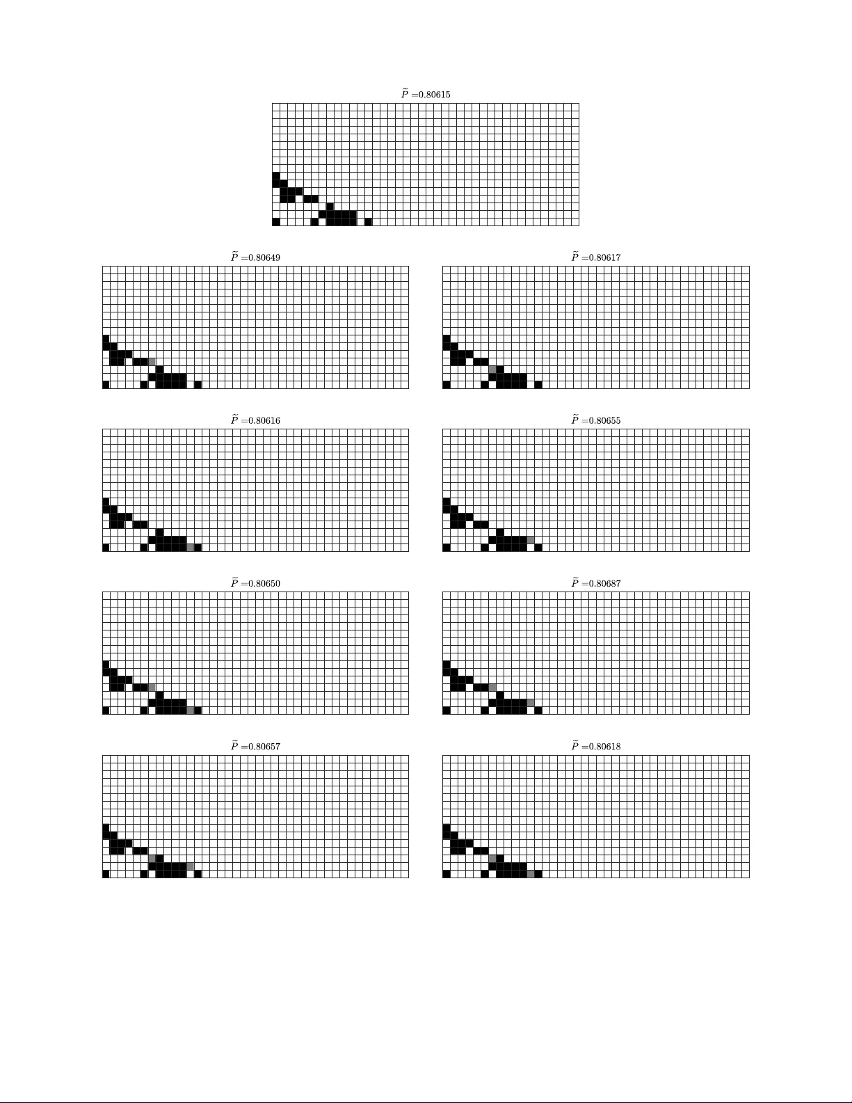
Self-Directed Online Mac hine Learning for T op ology Optimization Changyu Deng 1 , Yizhou W ang 2 , Can Qin 2 , Y un F u 2 , and W ei Lu 1,3,* 1 Departmen t of Mec hanical Engineering, Univ ersity of Michigan, Ann Arb or, MI 48109, United States 2 Departmen t of Electrical and Computer Engineering, Northeastern Universit y , Boston, MA 02115, United States 3 Departmen t of Materials Science and Engineering, Univ ersity of Michigan, Ann Arb or, MI 48109, United States * Corresp onding author: weilu@umic h.edu This pap er is published on Nature Communications ( https://rdcu.be/cFHgJ ) Abstract T op ology optimization by optimally distributing materials in a given domain requires non-gradien t optimizers to solve highly complicated problems. Ho wev er, with hundreds of design v ariables or more in volv ed, solving such problems would require millions of Finite Elemen t Metho d (FEM) calculations whose computational cost is h uge and impractical. Here w e rep ort Self-directed Online Learning Optimization (SOLO) which in tegrates Deep Neural Net work (DNN) with FEM calculations. A DNN learns and substitutes the ob jectiv e as a function of design v ariables. A small n um b er of training data is generated dynamically based on the DNN’s prediction of the optim um. The DNN adapts to the new training data and giv es b etter prediction in the region of interest un til conv ergence. The optim um predicted b y the DNN is pro ved to con verge to the true global optim um through iterations. Our algorithm was tested by four types of problems including compliance minimization, ﬂuid- structure optimization, heat transfer enhancement and truss optimization. It reduced the computational time by 2 ∼ 5 orders of magnitude compared with directly using heuristic metho ds, and outp erformed all state-of-the-art algorithms tested in our exp erimen ts. This approac h enables solving large m ulti-dimensional optimization problems. Main Distributing materials in a domain to optimize p erformance is a signiﬁcant topic in many ﬁelds, suc h as solid mec hanics, heat transfer, acoustics, ﬂuid mechanics, materials design and v arious m ultiphysics disciplines 1 . Man y n umerical approac hes 2 ha ve b een developed since 1988, where the problems are form ulated by density , level set, phase ﬁeld, top ological deriv ativ e or other metho ds 3 . T ypically , these approac hes use gradient-based optimizers, suc h as the Metho d of Mo ving Asymptotes (MMA), and th us hav e v arious restrictions on the prop erties of gov erning equations and optimization constraints to allow for fast computation of gradien ts. Because of the in trinsic limitation of gradien t-based algorithms, the ma jority of existing approac hes hav e only b een applied to simple problems, since they would fail as so on as the problem b ecomes 1 complicated suc h as in volving v arying signs on gradients or non-linear constrain ts 4 . T o address these diﬃculties, non-gradien t metho ds hav e b een dev elop ed which pla y a signiﬁcan t role in o vercoming the tendency to b e trapp ed in a lo cal minim um 5 . Non-gradien t optimizers, also known as gradien t-free or deriv ativ e-free metho ds, do not use the gradien t or deriv ativ e of the ob jectiv e function and has b een attempted b y sev eral researc hers, most of which are sto c hastic and heuristic metho ds. F or instance, Ha jela et al. applied Ge- netic Algorithm (GA) to a truss structure optimization problem to reduce weigh t 6 . Shim and Mano ochehri minimized the material use sub ject to maximum stress constraints by a Simulated Annealing (SA) approach 7 . Besides these tw o p opular metho ds, other algorithms hav e b een in vestigated as w ell, such as an t colonies 8,9 , particle swarms 10 , harmon y searc h 11 , and bacterial foraging 12 . Non-gradien t metho ds ha ve four adv an tages o ver gradient-based metho ds 5 : b etter optima, applicable to discrete designs, free of gradients and eﬃcien t to parallelize. How ev er, the ma jor disadv an tage of the metho ds is their high computational cost from calling the ob jectiv e functions, which b ecomes prohibitiv ely exp ensiv e for large systems 3 . As a trade-oﬀ, sometimes searc hing space can b e reduced in order for less computation. F or instance, pattern search has b een applied 13,14 whic h is a non-heuristic metho d with a smaller searching space but is more lik ely to b e trapp ed in lo cal minima. Mac hine learning has b een used in sequential mo del-based optimization (SMBO) to target at exp ensiv e ob jective function ev aluation 15,16 . F or instance, Bay esian optimization (BO) 17 uses a Gaussian prior to appro ximate the conditional probabilit y distribution of an ob jectiv e p ( y | x ) where y = F ( x ) is the ob jectiv e and x is the design v ariable (vector); then the unkno wn re- gions can b e estimated by the probability mo del. In Co v ariance Matrix Adaptation Evolution Strategy (CMA-ES) 18 , a m ultiv ariable Gaussian distribution is used to sample new queries. Ho wev er, as demonstrated later in the pap er, these methods are not designed for large-scale and high-dimensional problems, and thus do not p erform w ell in top ology optimization for slow con vergence 19 or requirement of shrinking design space 20 . Despite some improv emen t to scale up these algorithms 21,22 , none of them has shown sup erior p erformance in top ology optimization to the b est of our kno wledge. There are some reports on leveraging mac hine learning to reduce the computational cost of top ol- ogy optimization 23–31 . Most of them are generativ e mo dels which predict solutions of the same problem under diﬀeren t conditions, after b eing trained b y optimized solutions from gradient- based metho ds. F or example, Y u et al. 30 used 100,000 optimal solutions to a simple compliance problem with v arious b oundary forces and the optimal mass fractions to train a neural net w ork consisting of Conv olutional Neural Netw ork (CNN) and conditional Generativ e Adversarial Net- w ork (cGAN), whic h can predict near-optimal designs for an y giv en b oundary forces. How ev er, generativ e mo dels are not top ology optimization algorithms: they rely on existing optimal de- signs as the training data. The predictions are restricted b y the cov erage of the training datasets. T o consider diﬀeren t domain geometries or constrain ts, new datasets and netw orks w ould b e re- quired. Besides, the designs predicted by the net works are close to, but still diﬀerent from the optimal designs. An oﬄine learning metho d 31 replaces some FEM calculations during the op- timization pro cess with DNN’s prediction, y et giv es limited impro vemen t esp ecially considering that it requires the solutions to similar problems for training. 2 Here w e prop ose an algorithm called Self-directed Online Learning Optimization (SOLO) to accelerate non-gradien t top ology optimization. A DNN is used to map designs to ob jectives as a surrogate mo del to approximate and replace the original function whic h is exp ensiv e to calculate. A heuristic optimization algorithm ﬁnds the p ossible optimal design according to DNN’s prediction. Based on the optim um, new query p oin ts are dynamically generated and ev aluated by the Finite Element Metho d (FEM) to serv e as additional training data. The lo op of suc h self-directed online learning is repeated until conv ergence. This iterativ e learning sc heme, whic h can b e categorized as an SMBO algorithm, takes adv an tage of the searc hing abilities of heuristic metho ds and the high computational sp eed of DNN. Theoretical conv ergence rate is deriv ed under some assumptions. In con trast to gradient-based methods, this algorithm do es not rely on gradien t information of ob jective functions of the top ology optimization problems. This prop ert y allo ws it to b e applied to binary and discrete design v ariables in addition to contin uous ones. T o sho w its p erformance, w e test the algorithm by t wo compliance minimization problems (designing solid so that the structure achiev es maximum stiﬀness for a giv en loading), t wo ﬂuid- structure optimization problems (designing ﬂuid tunnel to minimize the ﬂuid pressure loss for a giv en inlet sp eed), a heat transfer enhancement problem (designing a copp er structure to reduce the charging time of a heat storage system), and three truss optimization problems (c ho osing the cross-sectional areas of bars in a truss). Our algorithm reduces the computational cost by at least tw o orders of magnitude compared with directly applying heuristic metho ds including Generalized Sim ulated Annealing (GSA), Binary Bat Algorithm (BBA) and Bat Algorithm (BA). It also outp erforms an oﬄine version (where all training data are randomly generated), BO, CMA-ES, and a recent algorithm based on reinforcemen t learning 32 . Results F ormulation and o v erview. Consider the following topology optimization problem: in a design domain Ω, ﬁnd the material distribution ρ ( x ) that could tak e either 0 (void) or 1 (solid) at p oin t x to minimize the ob jective function F , sub ject to a v olume constrain t G 0 ≤ 0 and p ossibly M other constrain ts G j ≤ 0( j = 1 , ..., M ) 4 . Mathematically , this problem can b e written as lo oking for a function ρ deﬁned on the domain Ω, min dom( ρ )=Ω F ( ρ )      G 0 ( ρ ) = R Ω ρ ( x ) d x − V 0 ≤ 0 G j ( ρ ) ≤ 0 , j = 1 , ..., M ρ ( x ) = 0 or 1 , ∀ x ∈ Ω , (1) where V 0 denotes the given volume. T o solve such a problem n umerically , the domain Ω is discretized in to ﬁnite elements to describ e the density distribution by N no dal or elemen tal 3 v alues, min ρ =[ ρ 1 ,ρ 2 ,...,ρ N ] T F ( ρ )          G 0 ( ρ ) = N P i =1 w i ρ i − V 0 ≤ 0 G j ( ρ ) ≤ 0 , j = 1 , ..., M ρ i ∈ S , i = 1 , ..., N , (2) where w i denotes the weigh t of in tegration. The domain of ρ i is usually binary ( S = { 0 , 1 } ), but more generally may tak e other v alues suc h as discrete ( S = { a 0 , a 1 , ..., a K } ) or con tinuous ( S = [0 , 1]). Our algorithm can b e applied to Eq.(2) with binary , discrete or contin uous design v ariables. In this section, w e discuss the case of contin uous design v ariables since it is most general. In many applications, the ob jective function is quite complicated and time-consuming to calcu- late, since it requires solving partial diﬀeren tial equations b y , for instance, FEM. T o reduce the n umber of FEM calculations and accelerate non-gradient optimization, w e build a DNN to ev al- uate the ob jective function. In a naiv e wa y , the en tire domain of the ob jective function should b e explored to generate the training data. This would incur a huge n um b er of FEM calculations. Ho wev er, we only care ab out the function v alues close to the global optim um and do not require precise predictions in irrelev ant regions. In other words, most information ab out the ob jective function in the domain is unnecessary except the details around the optimum. So we do not need to generate data to train in those irrelev an t regions. An intuitiv e explanation is shown in Fig. 1a. In a 1D minimization example, we can generate a small dataset to train the DNN and reﬁne the mesh around the minimum obtained from the curren t prediction to ac hieve higher resolution at the place of interest in the next iteration. After sev eral batc hes, the minim um of the predicted function would conv erge to that of the ob jective function. Fig. 1b sho ws the ﬂo w diagram of the prop osed algorithm. A small batch of random vectors (or arra ys) ρ satisfying the constraints in Eq.(2) is generated. The corresp onding ob jective v alues F ( ρ ) are calculated by FEM. Then, ρ and F ( ρ ) are inputted in to the DNN as the training data so that the DNN has a certain level of ability to predict the function v alues based on the design v ariables. Namely , the output of the DNN f ( ρ ) appro ximates the ob jectiv e function F ( ρ ). N ext, the global minimum of the ob jectiv e function f ( ρ ) is calculated by a heuristic algorithm. After obtaining the optimized array b ρ , more training data are generated accordingly . Inspired b y the concept of GA 33 , the disturbance w e add to the arra y is more than a small p erturbation, and is categorized as m utation, crosso v er and con v olution. Mutation means replacing one or sev eral design v ariables with random n um b ers; crossov er means exc hanging several v alues in the array; con volution means applying a con volution ﬁlter to the v ariables (see Metho ds for details). Then constrain ts are c hec ked and enforced. The self-directed learning and optimization pro cess stops when the v alue of the ob jective function F ( b ρ ) do es not c hange anymore or the computation budget is exhausted. This algorithm can con verge prov ably under some mild assumptions. Given the total num b er of 4 New data by disturbance minimum f 1 , DNN trained by data f 2 , DNN trained by data F , Objective function  (  )  a T rain DNN  ≈  Start Input objective function  & constraints Generate m 0 random  �  = argmin  (  ) Disturb �  t o generate m random  f Convergent? End Y Output �  N Initial data Calculate  (  ) New data Calculate  (  ) b Fig. 1: Sc hematics of the prop osed self-directed online learning optimization. a , Sc hematic illustration of self-directed online training. The initial batch of training data (light blue dots) is randomly lo cated. The DNN f 1 (dashed light-blue line) trained on ﬁrst batch of data only giv es a rough represen tation of the true ob jective function F (solid black line). The second batch training data (dark blue dots) are generated by adding disturbance (orange curve) to the minimum of f 1 . After trained with tw o batches, the DNN f 2 (dashed dark-blue line) is more reﬁned around the minim um (the region of interest), while remains almost the same at other lo cations suc h as the righ t con v ex part. f 2 is very close to ﬁnding the exact global minim um p oin t. b , Flow diagram of the algorithm. training data n train , for an y trained DNN with small training error, we ha ve [ F ( b ρ ) − F ∗ ] 2 ≤ e O  C √ n train  , (3) where C is a constant related to some inheren t prop erties of F and DNN, F ∗ is the global minim um of F , and e O omits log terms. This result states that when our trained DNN can ﬁt the training data well, then our algorithm can conv erge to the global optimal v alue. W e provid e con vergence guaran tee with concrete conv ergence rate for our prop osed algorithm, and to the b est of our kno wledge, this is the ﬁrst non-asymptotic conv ergence result for heuristic optimization metho ds using DNN as a surrogate mo del. The detailed theory and its deriv ation are elab orated in Supplementary Section 2. In the follo wing, we will apply the algorithm to eigh t classic examples of four t yp es (co vering binary , discrete and con tinuous v ariables): tw o compliance minimization problems, t wo ﬂuid- structure optimization problems, a heat transfer enhancement problem and three truss optimiza- tion problems. Compliance minimization. W e ﬁrst test the algorithm on t wo simple con tinuous compliance minimization problems. W e show that our algorithm can conv erge to global optim um and is 5 faster than other non-gradient metho ds. Symme t ry Roller Force a 0 500 1000 1500 2000 0.3 0.4 0.5 0.6 0.7 0.8 SOLO Offline SS GSA CMA-ES BO b 0 500 1000 1500 2000 -0.2 0 0.2 0.4 0.6 0.8 SOLO Offline c d Gradient-based e E = 0 . 293 e SOLO@501 e E = 0 . 298 f SOLO@5,782 e E = 0 . 293 0 0.2 0.4 0.6 0.8 1 Fig. 2: Setup and results of a compliance minimization problem with 5 × 5 design v ariables. a , Problem setup: minimizing compliance sub ject to maxim um v olume constrain t. b , Best dimensionless energy with a total of n train accum ulated training samples. SOLO denotes our prop osed metho d where the cross “X” denotes the conv ergence p oin t (presented in e ), “Oﬄine” denotes training a DNN oﬄine and then uses GSA to searc h for the optim um without up dating the DNN, whose results are indep enden t so they are plotted as circles instead of a curve, SS denotes Sto c hastic Searc h, which is the same as SOLO except that b ρ in eac h lo op is obtained b y the minimum of existing samples, CMA-ES denotes Cov ariance Matrix Adaptation Evolution Strategy , BO denotes Bay esian Optimization. SOLO conv erges the fastest among these methods. c , Energy prediction error of b ρ relative to FEM calculation of the same material distribution. e b ρ denotes DNN’s prediction, E b ρ denotes FEM’s result. d , Optimized design pro duced b y the gradien t-based metho d. e E = 0 . 293. e , Optimized design pro duced by SOLO. n train = 501 and e E = 0 . 298. f , Optimized design pro duced by SOLO. n train = 5 , 782 and e E = 0 . 293. In d - f , dark red denotes ρ = 1 and dark blue denotes ρ = 0, as indicated by the right color scale bar. As shown in Fig. 2a, a square domain is divided evenly b y a 4 × 4 mesh. A force down w ard is applied at the top right edge; the b ottom left edge is set as a roller (no v ertical displacement); the right b oundary is set to b e symmetric. There are 25 no dal design v ariables to control the material distribution, i.e. density ρ . Our goal is to ﬁnd the density ρ i ( i = 1 , 2 , ..., 25), sub ject to a volume constrain t of 0.5, such that the elastic energy E of the structure is minimized, 6 equiv alen t to minimizing compliance or the v ertical displacemen t where the external force is applied. F ormally , min ρ ∈ [0 , 1] N e E ( ρ ) = E ( ρ ) E ( ρ O ) , (4) where ρ O = [0 . 5 , 0 . 5 , ..., 0 . 5] T . The constraint is w · ρ ≤ 0 . 5 , (5) where w denotes the vector of linear Gaussian quadrature. In Eq.(4) we use the dimensionless elastic energy e E ( ρ ), deﬁned as the ratio of elastic energy of the structure with given material distribution to that of the reference uniform distribution (the material density is 0.5 everywhere in the domain). The elastic energy is calculated b y FEM from the Y oung’s mo dulus in the domain, whic h is related to densit y b y the p opular Simpliﬁed Isotropic Material with Penalization (SIMP) metho d, 34 Y ( ρ ( x )) = Y 0 ρ ( x ) 3 + ε  1 − ρ ( x ) 3  , (6) where Y and Y 0 denote the Y oung’s mo duli as a v ariable and a constan t resp ectiv ely , ε is a small n umber to av oid numerical singularity and ρ ( x ) is the material density at a giv en lo cation x in terp olated linearly b y the no dal v alues of the elemen t. F or b enc hmark, we use a traditional gradient-based algorithm, the Metho d of Mo ving Asymptotes (MMA), to ﬁnd the optimized solution (Fig. 2d). F or our prop osed metho d, we use 100 random arra ys to initialize the DNN. Then Generalized Sim ulated Annealing (GSA) is used to obtain the minimum b ρ based on the DNN’s prediction. Afterw ards, 100 additional samples will b e generated b y adding disturbance to b ρ including m u- tation and crosso ver. Suc h a lo op contin ues un til con v ergence. W e compare our prop osed metho d, Self-directed Online Learning Optimization (SOLO), with ﬁv e other algorithms. In Fig. 2b, SOLO conv erges at n train = 501. “Oﬄine” denotes a naive implemen tation to couple DNN with GSA, which trains a DNN oﬄine b y n train random samples and then uses GSA to search for the optimum, without up dating the DNN. As exp ected, the elastic energy decreases with the num b er of accumulated training samples n train . This is b ecause more training data will mak e the DNN estimate the elastic energy more accurately . Y et it con verges muc h slo w er than SOLO and do es not w ork well even with n train = 2 , 000. More results are sho wn in Supplementary Fig. 1. SS denotes Sto c hastic Searc h, whic h uses current minim um (the minimum of existing samples) to generate new searching samples; the setup is the same as SOLO except that the base design b ρ is obtained from the current minimum instead of a DNN. Comparing SS with SOLO, w e can conclude that the DNN in SOLO giv es a b etter searc hing direction than using existing optima. CMA-ES denotes Co v ariance Matrix Adaptation Ev olution Strategy with a m ulti-v ariable Gaussian prior. BO denotes Bay esian Optimization with Gaussian distribution as the prior and exp ected impro v ement (EI) as the acquisition function. Our metho d outp erforms all these metho ds in terms of con vergence sp eed. CMA-ES ranks the second with an ob jectiv e v alue 3% higher than SOLO at n train = 2 , 000. T o assess inference accuracy in online and oﬄine learning, w e compare the DNN-predicted energy with that calculated by FEM on the same material distribution. The relative error is deﬁned 7 b y [ e ( b ρ ) − E ( b ρ )] /E ( b ρ ) where e ( b ρ ) and E ( b ρ ) denote energy calculated by DNN and FEM re- sp ectiv ely . The energy prediction error is sho wn in Fig. 2c. When n train is small, b oth net works o verestimate the energy since their training datasets, comp osed of randomly distributed density v alues, corresp ond to higher energy . As n train increases, the error of SOLO ﬂuctuates around zero since solutions with lo w energy are fed bac k to the netw ork. Roller Symme t ry Force a 0 0.5 1 1.5 2 10 4 0.2 0.4 0.6 0.8 1 SOLO Offline CMA-ES b 0 0.5 1 1.5 2 10 4 -0.5 0 0.5 1 SOLO Offline c d Gradient-based e E = 0 . 222 e SOLO@10,243 e E = 0 . 228 f SOLO@77,691 e E = 0 . 222 0 0.2 0.4 0.6 0.8 1 Fig. 3: Setup and results of a compliance minimization problem with 11 × 11 design v ariables. a , Problem setup: minimizing compliance sub ject to maxim um v olume constrain t. b , Best dimensionless energy with a total of n train accum ulated training samples. SOLO denotes our prop osed metho d where the cross “X” denotes the conv ergence p oin t (presented in e ), “Oﬄine” denotes training a DNN oﬄine and then uses GSA to searc h for the optim um without up dating the DNN, whose results are indep enden t so they are plotted as circles instead of a curv e, CMA-ES denotes Co v ariance Matrix Adaptation Ev olution Strategy . SOLO conv erges the fastest among these metho ds. c , Energy prediction error of b ρ relative to FEM calculation of the same material distribution. e b ρ denotes DNN’s prediction, E b ρ denotes FEM’s result. d , Optimized design pro duced b y the gradien t-based metho d. e E = 0 . 222. e , Optimized design pro duced b y SOLO. n train = 10 , 243 and e E = 0 . 228. f , Optimized design pro duced by SOLO. n train = 77 , 691 and e E = 0 . 222. In d - f , dark red denotes ρ = 1 and dark blue denotes ρ = 0, as indicated b y the righ t bar. The solution of SOLO using 501 samples is presented in Fig. 2e, whose energy is 0.298, almost the same as that of the b enc hmark in Fig. 2d. With higher n train , the solution from SOLO b ecomes 8 closer to that of the b enc hmark (the ev olution of optimized structures is sho wn in Supplemen tary Fig. 2). In Fig. 2f, the energy is the same as the b enchmark. The material distribution in Fig. 2f do es not diﬀer m uch from that in Fig. 2e. In fact, using only 501 samples is suﬃcient for the online training to ﬁnd the optimized material distribution. W e ﬁnd that in our problem and optimization setting, the GSA needs ab out 2 × 10 5 function ev aluations to obtain the minimum of DNN. Since the DNN approximates the ob jective function, we estimate GSA needs the same n umber of ev aluations when applying to the ob jectiv e, then it means 2 × 10 5 FEM calculations are required if directly using GSA. F rom this p erspective, SOLO reduces the num b er of FEM calculations to 1/400. A similar problem with a ﬁner mesh having 121 (11 × 11) design v ariables is sho wn in Fig. 3a. The b enc hmark solution from MMA is shown in Fig. 3d, whose energy is 0.222. The trends in Fig. 3b and c are similar to those in Fig. 2 with a coarse mesh. Fig. 3b shows that SOLO con verges at n train = 10 , 243, giving e E = 0 . 228. Our metho d again outp erforms CMA-ES, the second b est algorithm according to Fig. 2b. The material distribution solutions are shown in Fig. 3e and f. The conﬁguration of SOLO is the same as that for the coarse mesh except that eac h lo op has 1,000 incremen tal samples and GSA p erforms 4 × 10 6 function ev aluations. Compared with directly using GSA, SOLO reduces the num b er of FEM calculations to 1/400 as well. The ev olution of optimized structures is shown in Supplementary Fig. 3. Fluid-structure optimization. In the following t wo problems, w e leverage our algorithm to address binary ﬂuid-structure optimization. W e wan t to show that our method outp erforms the gradien t-based method and a recen t algorithm based on reinforcemen t learning 32 . As shown in Fig. 4a, the ﬂuid enters the left inlet at a giv en velocity p erpendicular to the inlet, and ﬂows through the c hannel b ounded b y w alls to the outlet where the pressure is set as zero. In the 20 × 8 mesh, we add solid blocks to change the ﬂo w ﬁeld to minimize the friction loss when the ﬂuid ﬂo ws through the channel. Namely , we wan t to minimize the normalized inlet pressure min ρ ∈{ 0 , 1 } N e P ( ρ ) = P ( ρ ) P ( ρ O ) , (7) where P denotes the a verage inlet pressure and ρ O = [0 , 0 , ..., 0] T indicates no solid in the domain. As for the ﬂuid prop erties, w e select a conﬁguration with a lo w Reynolds num b er for stable steady solution 35 , sp eciﬁcally , Re = D v L µ = 40 , (8) where D denotes ﬂuid densit y , µ denotes viscosit y , v denotes inlet v elo cit y and L denotes inlet width (green line). F or the benchmark, we use a typical gradient-based algorithm which adds an imp ermeable medium to c hange binary v ariables to con tinuous ones 36 . It uses the adjoint metho d to de- riv e gradien ts and MMA as the solver. The solution is presen ted in Fig. 4c. The solid blo c ks form a ramp at the left b ottom corner for a smo oth ﬂow expansion. W e use tw o v ariants of our algorithm. One is denoted as SOLO-G, a greedy v ersion of SOLO where additional 10 samples pro duced in each lo op are all from the DNN’s prediction. The 9 Pressu re outlet V elocity inlet a 0 500 1000 1500 2000 2500 0.96 0.97 0.98 0.99 1 Gradient-based SOLO-G SOLO-R 280 290 0.9565 0.957 0.9575 2140 2150 0.9567 0.9568 0.9569 0.957 b c Gradient-based e P = 0 . 9569 1 2 3 4 5 6 7 8 9 10 11 12 13 14 15 16 17 18 19 20 1 2 3 4 5 6 7 8 d SOLO-G@286 e P = 0 . 9567 1 2 3 4 5 6 7 8 9 10 11 12 13 14 15 16 17 18 19 20 1 2 3 4 5 6 7 8 e SOLO-R@2,148 e P = 0 . 9567 1 2 3 4 5 6 7 8 9 10 11 12 13 14 15 16 17 18 19 20 1 2 3 4 5 6 7 8 Fig. 4: Setup and results of a ﬂuid-structure optimization problem with 20 × 8 design v ariables. a , Problem setup: minimizing pressure drop through the tunnel. The v ertical green line on the left denotes the inlet while the v ertical blue line on the right denotes the outlet. b , Dimensionless inlet pressure versus n train , the n um b er of accum ulated training samples. SOLO- G denotes a greedy v ersion of our prop osed metho d, SOLO-R denotes the regular version of our prop osed metho d. The horizontal dashed line denotes the solution from the gradien t-based metho d. The cross “X” denotes the con v ergence p oin t (presen ted in d and e , resp ectively). c , Optimized design obtained b y the gradient-based metho d. e P = 0 . 9569. d , Optimized design obtained by SOLO-G. n train = 286 and e P = 0 . 9567. e , Optimized design obtained by SOLO-R. n train = 2 , 148 and e P = 0 . 9567. In c - e , black denotes ρ = 1 (solid) and white denotes ρ = 0 (v oid). The solutions in d and e are equiv alen t since the ﬂow is blo c ked b y the black squares forming the ramp surface and the white squares within the ramp at the left b ottom corner are irrelev an t. initial batc h is comp osed of a solution ﬁlled with zeros and 160 solutions each of which has a single elemen t equal to one and others equal to zero. The pressure v alues corresp onding to these designs are calculated by FEM. These 161 samples are used to train a DNN. Next, Binary Bat Algorithm (BBA) is used to ﬁnd the minim um of the DNN. The top 10 solutions (after removing rep eated ones) encountered during BBA searching will b e used as the next batc h of training data. The other v ariant, denoted as SOLO-R, is a regular version of SOLO where each lo op has 100 incremental samples. 10 of them are pro duced in the same wa y as SOLO-G whereas the rest 90 are generated by adding disturbance to the b est solution predicted by the DNN. Similar to the compliance minimization problems, the disturbance includes m utation and crossov er. As shown in Fig. 4b, SOLO-G and SOLO-R con verge to the same ob jective function v alue e P = 0 . 9567 at n train = 286 and n train = 2 , 148 resp ectiv ely . Their solutions are equiv alent, sho wn in Fig. 4d and e. In termediate solutions from SOLO-G are shown in Supplementary Fig. 4. W e obtain the optim um b etter than the gradient-based metho d ( e P = 0 . 9569) after only 286 FEM calculations. F or comparison, a recent topology optimization work based on reinforcemen t learn- 10 Pressu re outlet V elocity inlet a 0 500 1000 1500 2000 2500 0.8 0.82 0.84 Gradient-based SOLO-G 1900 1910 1920 0.8062 0.8064 b c Gradient-based e P = 0 . 8065 1 2 3 4 5 6 7 8 9 10 11 12 13 14 15 16 17 18 19 20 21 22 23 24 25 26 27 28 29 30 31 32 33 34 35 36 37 38 39 40 1 2 3 4 5 6 7 8 9 10 11 12 13 14 15 16 d SOLO-G@1,912 e P = 0 . 8062 1 2 3 4 5 6 7 8 9 10 11 12 13 14 15 16 17 18 19 20 21 22 23 24 25 26 27 28 29 30 31 32 33 34 35 36 37 38 39 40 1 2 3 4 5 6 7 8 9 10 11 12 13 14 15 16 Fig. 5: Setup and results of a ﬂuid-structure optimization problem with 40 × 16 design v ariables. a , Problem setup: minimizing pressure drop through the tunnel. b , Dimensionless inlet pressure versus n train , the num b er of accumulated training samples. SOLO-G denotes a greedy version of our prop osed metho d, where the cross “X” denotes the conv ergence p oin t (pre- sen ted in d ). The horizon tal dashed line denotes the solution from the gradient-based metho d. c , Optimized design obtained b y the gradient-based metho d. e P = 0 . 8065. d , Optimized design obtained by SOLO-G. n train = 1 , 912 and e P = 0 . 8062. In c , d , blac k denotes ρ = 1 (solid) and white denotes ρ = 0 (v oid). The SOLO-G result in d has tw o gaps at the 7th and 12th columns, while the gradien t-based result in c giv es a smo oth ramp. W e try ﬁlling the gaps and ﬁnd that their existence indeed reduces pressure, which demonstrates the p o werfulness of our metho d. ing used the same geometry setup and obtained the same solution as the gradient-based metho d after thousands of iterations 32 ; our approach demonstrates b etter p erformance. Compared with directly using BBA which requires 10 8 ev aluations, SOLO-G reduces FEM calculations by or- ders of magnitude to ab out 1 / (3 × 10 5 ). T o accoun t for randomness, we rep eat the exp eriments another four times and the results are similar to Fig. 4b (see Supplementary Figs. 5 and 6). W e also apply our algorithm to a ﬁner mesh, with 40 × 16 design v ariables (Fig. 5a). SOLO-G con verges at n train = 1 , 912, shown in Fig. 5b. Our design (Fig. 5d, e P = 0 . 8062) is found to b e b etter than the solution from the gradien t-based algorithm (Fig. 5c, e P = 0 . 8065). In termediate solutions from SOLO-G are shown in Supplementary Fig. 7. Compared with directly using BBA whic h needs 2 × 10 8 ev aluations, SOLO-G reduces the num b er of FEM calculations to 1 / 10 5 . Similar trends can b e observ ed when rep eating the exp erimen ts (see Supplementary Fig. 7). It is in teresting to note that the optimum in Fig. 5d has tw o gaps at the 7th and 12th columns. It is a little counterin tuitiv e, since the gradien t-based metho d gives a smo oth ramp (Fig. 5c). W e try ﬁlling the gaps and ﬁnd that their existence indeed reduces pressure (see Supplementary Fig. 8), whic h demonstrates how p o werful our metho d is. 11 Heat transfer enhancement. In this example, w e w ould lik e to solv e a complicated problem that gradient-based metho ds are diﬃcult to address. Phase change materials are used for energy storage by absorbing and releasing latent heat when the materials c hange phases, typically b e- t ween solid and liquid. Due to their simple structure and high heat storage capacity , they are widely used in desalination, buildings, refrigeration, solar system, electronic co oling, spacecraft and so forth 37 . Ho w ever, commonly used non-metallic materials suﬀer from v ery low thermal conductivit y . A p opular solution is to add high conductivity material (suc h as copp er) as ﬁns to enhance heat transfer 38 . T op ology optimization is implemen ted to optimize the geometry of ﬁns. T o deal with such transien t problems, current gradient-based metho ds hav e to simplify the problem b y using predetermined time p erio d and ﬁxed boundary conditions 39–42 . By contrast, in real applications, these conditions dep end on user demand and en vironment, or even couple with the temp erature ﬁeld of the energy storage system 43–47 . Therefore, problems with more complex settings need to b e addressed. W e consider a heat absorption scenario where time is v ariant and the b oundary condition is coupled with the temp erature ﬁeld. As shown in Fig. 6a, copp er pip es con taining heat source are inserted in a phase c hange material, paraﬃn w ax R T54HC 48 ; the heat source can be fast-c harging batteries for electric vehicles or hot water for residen tial buildings. Considering symmetry , the problem is conv erted to a 2D problem in Fig. 6b. W e ﬁll the domain with wax to store heat and with copp er to enhance heat transfer. The material distribution ρ ( x ) ∈ { 0 , 1 } (1 b eing copp er and 0 b eing wax) is represented by a 10 × 10 mesh. Sp eciﬁcally , a contin uous function is interpolated by Gaussian basis functions from the 10 × 10 design v ariables and then conv erted to binary v alues b y a threshold (see Metho ds for details). Our goal is to ﬁnd the optimal ρ to minimize the time to c harge the system with a given amoun t of heat min ρ ∈ [0 , 1] N e t ( ρ ) = t ( ρ ) t ( ρ O ) , (9) where N = 100, ρ O = [0 , 0 , .., 0] T means no copp er inside the design domain, and t ( ρ ) is the time to c harge the system with Q 0 amoun t of heat, expressed b y Z t ( ρ ) 0 q ( ρ , t )d t = Q 0 , (10) sub ject to the maxim um heat ﬂux constraint at the b oundary (green curve in Fig. 6b) q ( ρ , t ) ≤ q 0 , (11) the constraint of maximum temp erature of the domain, T ( ρ , q , x , t ) ≤ T 0 , (12) and given copp er usage, i.e., the volume constrain t of copp er, R Ω ρ ( x )d x R Ω d x = 0 . 2 . (13) 12 a Heat flux Adiabatic Design domain Copper (copper and wax) b 0 0.5 1 1.5 2 2.5 10 4 0 0.05 0.1 0.15 0.2 SOLO Direct Approximated c d SOLO@20,860 e t = 0 . 0137 e Direct@24,644 e t = 0 . 0275 f Approximated e t = 0 . 0203 Fig. 6: Setup and results of a heat transfer enhancemen t problem with 10 × 10 design v ariables. a , Engineering bac kground: a group of copp er pip es are inserted in a phase change material. Because of symmetry , we only need to consider 1/8 of the unit cell (dark blue area in the top right corner). b , Problem setup: minimizing the time to c harge the system with a giv en amoun t of heat, sub ject to heat ﬂux, temp erature and v olume constrain ts. The blac k dots denote lo cations of design v ariables. c , Dimensionless c harging time versus n train , the num b er of accumulated training samples. SOLO denotes our prop osed metho d, where the cross “X” denotes the con vergence p oin t (presented in d ). “Direct” denotes solving the problem directly b y gradient descen t. “Appro ximated” denotes simplifying this problem to a steady state problem. d , Optimized design obtained b y SOLO. e t = 0 . 0137. e , Optimized design obtained b y “Direct”. n train = 24 , 644 and e t = 0 . 0275. f , Optimized design obtained b y “Approximated”. e t = 0 . 0203. In d - f , blac k denotes ρ = 1 (copp er) and white denotes ρ = 0 (w ax). The SOLO result in d has islands isolated from ma jor branches, while the “Approximated” result in f giv es a connected structure. W e try combining the islands to b e part of ma jor branc hes and ﬁnd that the existence of isolated islands indeed reduces time, which demonstrates the p o w erfulness of our metho d. Here Q 0 , q 0 and T 0 are preset constants. Ob viously , the b ottom left b oundary (inner side of copp er pip es) has the highest temp erature during charging, thus we only need to consider the temp erature constraint at this b oundary . Ph ysically , there are one or tw o charging steps: the system is c harged at heat ﬂux q 0 un til the b oundary temp erature reaches T 0 or the total heat ﬂo w reaches Q 0 (whic hever ﬁrst), and if it is the former case, the heat ﬂux is reduced to maintain the b oundary temp erature at T 0 un til the total heat ﬂow requiremen t is satisﬁed. In practice, w e c ho ose parameters such that the system will go through t wo steps for sure. 13 T o solve the problem with ob jectiv e Eq.(9) and constrain ts in Eqs.(11)-(13), our metho d SOLO is initialized by 500 random samples to train a DNN. Bat Algorithm (BA) is then used to ﬁnd the minimum of the DNN, based on whic h additional 200 samples are generated in each lo op b y m utation and con v olution. Two gradient-based metho ds are used as baselines to compare with our algorithm: one is to solv e Problem (9)-(13) directly b y gradien t descen t, denoted as “Direct”; the other is to simplify this problem to a steady state problem 42 , denoted as “Appro ximated”. In Fig. 6c, SOLO conv erges at n train = 20 , 860 (mark ed by a cross “X”) with low er e t than other metho ds. It app ears coun ter-intuitiv e that the solution of SOLO, shown in Fig. 6d, has some copp er islands isolated from ma jor branc hes. W e tried removing these islands and adding more copp er materials to the ma jor branc hes to maintain copp er volume, yet the v ariants show ed w orse p erformance, as shown in Supplementa ry Fig. 10. “Direct” giv es the worst solution in Fig. 6e. “Approximated” yields a go o d solution with a tree structure, as sho wn in Fig. 6f; since it do es not solv e the same problem as the other tw o metho ds, we do not consider its relation with n train and represent it by a horizontal line in Fig. 6c. Our metho d gives a go o d solution after 20,860 FEM calculations, while BA is estimated to need 4 × 10 8 calculations. In summary , our metho d outp erforms the other tw o metho ds and reduces the num b er of FEM calculations b y o ver four orders of magnitude compared with BA. T russ optimization. In this example, we test the scalabilit y of SOLO with ov er a thousand design v ariables. Also, w e will compare it with a heuristic metho d, BA, to pro vide direct evidence that SOLO can reduce the num b er of FEM computations b y ov er tw o orders of magnitude. T russ structures are widely used in bridges, tow ers, buildings and so forth. An exemplary ap- plication, an antenna to wer, is sho wn in Fig. 7a. Researc hers hav e b een w orking on optimizing truss structures from diﬀeren t p ersp ectiv es. A classic truss optimization b enc hmark problem is to optimize a structure with 72 bars 49–52 , as sho wn in Fig. 7b with four rep eated blo c ks, so as to minimize the weigh t of the bars sub ject to displacement and tension constrain t. F ollo wing this benchmark problem, we set the goal to optimize the size of eac h bar (the bars can all ha ve diﬀeren t sizes) to minimize total dimensionless w eight min ρ ∈{ a 1 ,a 2 ,...,a 16 } N f W ( ρ ) = W ( ρ ) W ( ρ max ) = P N i =1 ρ i L i γ i W ( ρ max ) , (14) where ρ i , L i and γ i are the cross-sectional area, length, and unit w eigh t of the i -th bar, resp ec- tiv ely; ρ max uses the largest cross-sectional area for all bars; N = 72 is the num b er of bars. Eac h bar is only allo wed to c ho ose from 16 discrete cross-sectional area v alues a 1 , a 2 , ..., a 16 , to represen t standardized comp onen ts in engineering applications. The tension constrain t requires all bars to not exceed the maximum stress | σ i | ≤ σ 0 , i = 1 , 2 , ..., N . (15) The displacement constrain t is applied to the connections of the bars: the displacemen t in an y direction is required to be lo wer than a threshold || ∆ x i || ∞ ≤ δ 0 , i = 1 , 2 , ..., N c , (16) 14 a Force b c 72 bars 1 0 3 1 0 4 1 0 5 0 . 1 0 . 2 0 . 3 S O L O B A ≈ 1 0 2 t i m e s d 432 bars 1 0 3 1 0 4 1 0 5 1 0 6 1 0 7 1 0 8 0 . 1 0 . 2 0 . 3 0 . 4 ≈ 3 × 1 0 3 t i m e s S O L O B A e 1,008 bars 1 0 4 1 0 5 1 0 6 1 0 7 1 0 8 0 . 1 5 0 . 2 0 0 . 2 5 0 . 3 0 S O L O B A ≈ 3 × 1 0 3 t i m e s Fig. 7: Setup and results of three truss optimization problems with diﬀerent num b ers of bars (equal to the num b ers of design v ariables). a , Illustration of an antenna to wer, an exemplary application of truss structures. b , Illustration of the problem setup: minimizing total w eight through changing the size of each bar, sub ject to stress and displacemen t constraints. The blo c k is rep eated un til the giv en n umber of bars is reached. c - e , Dimensionless w eight f W v ersus the n umber of accum ulated training samples n train . SOLO denotes our prop osed metho d. BA denotes Bat Algorithm. The num b ers of bars for these three sub-ﬁgures are 72, 432 and 1,008, resp ectiv ely . Eac h exp eriment is rep eated ﬁve times; the curves denote the mean and the shado ws denote the standard deviation. where N c is the n umber of connections. No w w e ha ve an optimization problem with ob jective Eq.(14) sub ject to stress constrain t Eq.(15) and displacement constraint Eq.(16). In addition to the p opular 72-bar problem, w e add more rep eated blo c ks to the structure to generate t wo more problems, with 432 and 1,008 bars. Geo- metric symmetry is not considered while solving the problems. Therefore, the design space go es up to 16 1 , 008 ≈ 10 1 , 214 , whic h is extremely huge. F or the three problems, SOLO is initialized by 100, 500 and 1,000 samples, resp ectiv ely . The n umber of incremental samples p er lo op is 10% of the initialization samples. 10% of incremental samples are the optima obtained b y BA based on the DNN’s prediction, and the rest 90% are generated by m utation of the b est solution predicted b y the DNN. 15 The results are shown in Fig. 7c-e. T o reac h the same ob jective weigh t, BA needs ov er 10 2 times of calculations of SOLO. The diﬀerence b ecomes even larger when the n umber of v ariables increases. These examples demonstrate the scalabilit y of SOLO by sho wing higher eﬃciency in computation, esp ecially with a large n umber of design v ariables. Discussion T op ology optimization is an imp ortan t problem with broad applications in many scien tiﬁc and engineering disciplines. Solving non-linear high-dimensional optimization problems requires non- gradien t metho ds, but the high computational cost is a ma jor challenge. W e prop osed an approac h of self-directed online learning optimization (SOLO) to dramatically accelerate the optimization pro cess and mak e solving complex optimization problems p ossible. W e demonstrated the eﬀectiveness of the approac h in solving eigh t problems of four types, i.e., t wo compliance minimization problems, tw o ﬂuid-structure optimization problems, a heat transfer enhancemen t problem and three truss optimization problems. F or the compliance problems with 25 and 121 contin uous design v ariables, our approac h conv erged and pro duced optimized solutions same as the known optima with only 501 and 10,243 FEM calculations, resp ectiv ely , whic h are ab out 1/400 of directly using GSA and FEM without DNN based on our estimation. F or the ﬂuid problems with 160 and 640 binary v ariables, our metho d (SOLO-G) con v erged after 286 and 1,912 FEM calculations, resp ectiv ely , with solutions b etter than the b enc hmark. It used less than 1 / 10 5 of FEM calculations compared with directly applying BBA to FEM, and con verged m uch faster than another w ork based on reinforcement learning. In the heat transfer enhancemen t example, w e inv estigated a complicated, transien t and non-linear problem. Our metho d gav e a solution that outp erformed other baselines after 20,860 FEM calculations, whic h w as estimated to b e four orders of magnitude less than BA. Similar to other SMBO metho ds, o verhead computation was introduced (b y training DNNs and ﬁnding their optima), but it w as almost negligible (see the time proﬁle in Supplemen tary T able 1) whic h is attractive for real- w orld applications where new designs wan t to b e developed and tested. In these examples, w e estimated the amount of computation of directly using heuristic algorithms, which show ed that our approac h led to 2 ∼ 5 orders of magnitude of computation reduction. In addition to this estimation, w e applied BA to the original ob jectiv es in the three truss optimization problems and observed 2 ∼ 4 orders of magnitude of calculation reduction using our approac h. Our algorithm is neat and eﬃcien t, and has great p oten tial for large-scale applications. W e bring a new p erspective for high-dimensional optimization by em b edding deep learning in optimiza- tion metho ds. More tec hniques, suc h as parallel FEM computation, uncertaint y mo deling and disturbance based on sensitivity analysis, can b e incorp orated to enhance the p erformance. Metho ds Enforcemen t of v olume constraint. Compliance and heat transfer problems ha ve v olume constrain ts. The latter will b e detailed in Section Interp olation of design variables , thus w e only discuss the former here. In the t wo compliance problems, all matrices represen ting the densit y 16 distribution ρ ha ve the same weigh ted av erage P N i =1 w i ρ i = V 0 due to the volume constraint where w i denotes the weigh t of linear Gaussian quadrature. A matrix from the initial batc h is generated by three steps: 1. Generate a random matrix with elements uniformly distributed from 0 to 1. 2. Rescale the arra y to enforce the predeﬁned weigh ted av erage. 3. Set the elements greater than one, if an y , to one and then adjust those elements less than one to main tain the a verage. Matrices for the second batc h and afterwards add random disturbance to optimized solutions b ρ and then go through Step 2 and 3 ab o ve to mak e sure the v olume satisﬁes the constraint. Finite Element Metho d (FEM) and gradient-based baselines. The ob jective function v alues of material designs are calculated b y FEM as the ground truth to train the DNN. In the compliance and ﬂuid problems, the meshes of FEM are the same as the design v ariables. In the heat problem, the meshes are ﬁner. Numerical results are obtained b y COMSOL Multiphysics 5.4 (except the truss problems). Solutions from gradien t-based metho ds (including “Approximated” ) are all solved b y MMA via COMSOL with optimality tolerance as 0.001. In the ﬂuid problems, the gradien t-based baseline metho d pro duces a contin uous arra y , and w e use multiple thresholds to conv ert it to binary arrays and recompute their ob jective (pressure) to select the b est binary arra y . In the heat problem, the “Appro ximated” metho d uses the same resolution as the other t wo metho ds (SOLO and “Direct”) for a fair comparison. Sp eciﬁcally , we apply a Helmholtz ﬁlter 53 , whose radius is half of the minimum distance of t wo design v ariable lo cations, to yield a mesh-indep enden t solution. The solution is a contin uous arra y; w e use a threshold to conv ert it to a binary array which satisﬁes the v olume constrain t in Eq.(14). In terp olation of design v ariables. In the t wo compliance problems and the heat problem, w e use a v ector (or matrix) ρ to represent a spacial function ρ ( x ). In terp olation is needed to obtain the function ρ ( x ) for FEM and plotting. Given design v ariables ρ = [ ρ 1 , ρ 2 , ..., ρ N ] T , we get the v alues ρ ( x ) by tw o in terp olation metho ds. F or the compliance problems, we use bilinear in terp olation 54 . Supp ose x = ( x, y ) is within a rectangular elemen t whose no dal co ordinates are ( x 1 , y 1 ) , ( x 1 , y 2 ) , ( x 2 , y 1 ) , ( x 2 , y 2 ), the in terp olated function v alue can b e calculated b y ρ ( x, y ) =  x 2 − x x − x 1   F ( x 1 , y 1 ) F ( x 1 , y 2 ) F ( x 2 , y 1 ) F ( x 2 , y 2 )   y 2 − y y − y 1  ( x 2 − x 1 )( y 2 − y 1 ) . (17) F or the heat problem, a contin uous function ¯ ρ ( x ) ∈ [0 , 1] (which will later b e conv erted to a binary function whic h takes 0 or 1) is in terp olated by Gaussian basis functions 13,20 : ¯ ρ ( x, y ) = N X i =1 λ i φ ( x , x i ) + a 0 + a 1 x + a 2 y , (18) where φ ( x , x i ) = e − ( x − x i ) 2 /d 2 ( d is a preset distance), and λ i , a 0 , a 1 , a 2 are parameters to b e 17 determined. The following constrain ts are needed to guaran tee a unique solution N X i =1 λ i = 0 , N X i =1 λ i x i = 0 , N X i =1 λ i y i = 0 . (19) Expressing the ab o ve equations by a matrix form, we ha ve          φ ( x 1 , x 1 ) . . . φ ( x 1 , x N ) 1 x 1 y 1 . . . . . . . . . . . . . . . . . . φ ( x N , x 1 ) . . . φ ( x N , x N ) 1 x N y N 1 . . . 1 0 0 0 x 1 . . . x N 0 0 0 y 1 . . . y N 0 0 0                   λ 1 . . . λ N a 0 a 1 a 2          =          ρ 1 . . . ρ N 0 0 0          , (20) abbreviated as Φ λ =  ρ 0  . W e get λ = Φ − 1  ρ 0  and in terp olate ¯ ρ ( x ) b y Eq.(18). Then we set a threshold ρ thres to con vert the con tinuous function ¯ ρ ( x ) to a binary one ρ ( x ) ∈ { 0 , 1 } , i.e., ρ ( x ) = 1 if ¯ ρ ( x ) ≥ ρ thres and ρ ( x ) = 0 otherwise. The threshold ρ thres is controlled to satisfy the copp er v olume constrain t Eq.(13). Deep Neural Net w ork (DNN). The architectures of the DNN used in this pap er is presen ted in Fig. 8. The design v ariable ρ is ﬂattened to a 1D v ector as the input to DNN. All inputs are normalized b efore training and we introduce batch normalization (BN) 55 within the netw ork as regularization. The output of DNN is recipro cal of the ob jectiv e function (energy , pressure, c harging time or w eigh t) to giv e b etter resolution at low er ob jective v alues. F or the rest of this pap er, we regard the DNN to approximate the ob jective function for simplicity . T o optimize the DNN training pro cess, we apply ADAM 56 as the optimizer implemented on the platform of PyT orch 1.8.0 57 . The learning rate is 0.01. The loss function is set as Mean Square Error (MSE) 58 . All mo dels are trained for 1,000 ep o c hs with a batch size of 1,024 (if the num b er of training data is less than 1,024, all the data will b e used as one batc h). Random generation of new samples from a base design. After calculating the optimized arra y b ρ , more training data are generated by adding disturbance to it. As shown in Fig. 9, there are three kinds of disturbance: mutation, crossov er and conv olution. They are all likely to c hange the w eighted av erage of an array , thus the enforcement of v olume constraint will b e applied when necessary . Mutation means mutating several adjacent cells in the optimized array , i.e., generating random n umbers from 0 to 1 to replace the original elements. In the 2D example sho wn in Fig. 9a, the n umbers in a 2-b y-2 b o x are set as random. Crossov er denotes the crosso ver of cells in the arra y b ρ and is achiev ed b y the following steps: 1. Assign a linear index to each element in the arra y . 2. Randomly pick sev eral indices. 3. Generate a random sequence of the indices. 18 Linear , N × 512 BatchNorm 1d Leaky ReLU Linear , 512 × 256 Dropout BatchNorm 1d Leaky ReLU Linear , 256 × 128 BatchNorm 1d Dropout Leaky ReLU Linear , C × C Dropout BatchNorm 1d Leaky ReLU Linear , C × C BatchNorm 1d × B × B Linear , 128 × 1 Linear , 256× 256 Dropout BatchNorm 1d Linear , N × C BatchNorm 1d Leaky ReLU Linear Dropout BatchNorm 1d Leaky ReLU Linear , 256 × 128 BatchNorm 1d Dropout Leaky ReLU Linear , 128 × 1 Linear , N × C Dropout BatchNorm 1d Leaky ReLU Linear , C × C /2 BatchNorm 1d Leaky ReLU Linear , C /2× 1  ∈ 0 , 1  N = 25 / 12 1  ∈ 0 , 1   = 1 00  ∈  0 ,  1 , … ,  1 6   = 72 / 43 2 / 1 , 0 08  (  )  (  )  (  ) a b c  ∈ 0 , 1   = 16 0 / 64 0 or Fig. 8: Arc hitectures of DNN. The input is a design v ector ρ and the output is the predicted ob jective function v alue f ( ρ ).“Linear” presents a linear transformation and “Batc hNorm1d” denotes one-dimensional batch normalization used to av oid in ternal cov ariate shift and gradient explosion for stable training 55 . “LeakyReLU” is an activ ation function extended from ReLU with activ ated negativ e v alues. “Dropout” is a regularization metho d to preven t ov erﬁtting b y randomly masking no des 59 . a , the DNN in the compliance and ﬂuid problems. b , the DNN in the heat problem. Tw o arc hitectures are used in this problem. At the 100th lo op and b efore, B = 1, C = 512, and the Linear lay er in the dashed b o x is 512 × 256. A t the 101st lo op and afterw ards, B = 4, C = 512 and the 4 Linear la yers are 256 × 512, 512 × 512, 512 × 512 and 512 × 256, resp ectiv ely . c , the DNN in the truss optimization problems. B = 1. C = 512 when N = 72 / 432; C = 1 , 024 when N = 1 , 008. 4. Replace the original n um b ers according to the sequence ab o v e. As sho wn in Fig. 9b, indices are assigned sequentially from left to righ t and from top to b ottom. The indices we pick in Step 2 are 3, 4 and 8; the sequence generated in Step 3 is 4, 8 and 3. In the tw o compliance problems, the wa ys to generate a new input matrix based on b ρ and their p ossibilities are: (a) m utation: mutating one element in b ρ (10%); 19 1 2 3 4 5 6 7 8 9 1 2 3 1 2 6 8 6 9 1 2 3 4 5 6 7 8 9 1 2 4 8 5 6 7 3 9 Exchange numbers 1 2 3 4 5 6 7 8 9 1 2 3 53 36 6 52 32 9 1 2 3 4 * Replace with random numbers Convolution a b c Fig. 9: Illustration of m utation and crossov er . a , An example of m utation: some adjacen t cells (in the red b o x) are replaced with random num b ers. b , An example of crossov er: several cells (in the red b o xes) are exc hanged. c , An example of con volution: several cells (in the red b o x) are conv oluted with a kernel (in the blue cell). The volume constrain t may b e enforced at next step, not shown here. (b) m utation: mutating a 2 × 2 matrix in b ρ (10%); (c) m utation: mutating a 3 × 3 matrix in b ρ (20%); (d) m utation: mutating a 4 × 4 matrix in b ρ (20%); (e) crosso ver: choosing an integer n from one to the num b er of total elements, selecting n cells in b ρ and p erm uting them (20%); (f ) generating a completely random matrix like the initial batc h (20%). In the ﬂuid problem with 20 × 8 mesh, i.e. SOLO-R, the w ays are the same as previous ones except a threshold is needed to con vert the contin uous array in to a binary one. The threshold has 50% probability to b e β 4 1 where β 1 is uniformly sampled from [0 , 1], and has 50% probabilit y to b e the elemen t-wise mean of b ρ . In the heat problem, crossov er is replaced b y con v olution. It is the same as the compliance problems except that (e) ab o ve is replaced b y (g) Con volution: substituting a submatrix of the array , whose size and the corresp onding probabilit y is the same as (a-d), with a same c onvolution (the output has the same size as the input submatrix) b et w een the submatrix and 2 × 2 kernel whose elemen t is uniformly sampled from [0 , 1]. In the truss optimization problems, the design v ariable ρ is purely one-dimensional and can no longer b e represen ted as a matrix. Therefore, we only use m utation. First, β 2 is uniformly sampled from [0 , 1] to indicate the ratio of elements to b e mutated in b ρ , and then those elements are randomly selected to add γ to themselv es; γ is uniformly sampled from [ − 1 , 1]. Generalized Simulated Annealing (GSA). Simulated Annealing (SA) is a stochastic metho d 20 to determine the global minim um of a ob jective function b y simulating the annealing process of a molten metal 60 . GSA is a type of SA with sp eciﬁc forms of visiting function and acceptance probabilit y 61 . Assuming ob jective b ρ = arg min ρ ∈ [0 , 1] N h ( ρ ) , (21) w e do the following: 1. Generate an initial state ρ (0) = [ ρ (0) 1 , ρ (0) 2 , ..., ρ (0) N ] T randomly and obtain its function v alue E (0) = h ( ρ (0) ). Set parameters T (0), t max , q v , q a . 2. F or artiﬁcial time step t = 1 to t max , (a) Generate a new state ρ ( t ) = ρ ( t − 1) + ∆ ρ ( t ) , where the probability distribution of ∆ ρ ( t ) follo ws the visiting function g (∆ ρ ( t ) ) ∝ [ T ( t )] − N 3 − q v  1 + ( q v − 1) [∆ ρ ( t ) ] 2 [ T ( t )] 2 3 − q v  1 q v − 1 + N − 1 2 . (22) where T denotes the artiﬁcial temperature calculated by T ( t ) = T (0) 2 q v − 1 − 1 (1 + t ) q v − 1 − 1 . (23) (b) Calculate the energy diﬀerence ∆ E = E ( t ) − E ( t − 1) = h ( ρ ( t ) ) − h ( ρ ( t − 1) ) . (24) (c) Calculate the probabilit y to accept the new state p = min ( 1,  1 − (1 − q a ) t T ( t ) ∆ E  1 1 − q a ) . (25) Determine whether to accept the new state based on the probability , if not, ρ ( t ) = ρ ( t − 1) . 3. Conduct lo cal search to reﬁne the state. Since compliance minimization has a v olume constraint, the ob jective function used in the opti- mization pro cess is written as h ( ρ ) = f ( ρ ) + c ( w · ρ − V 0 ) 2 , (26) where c is a constant to transform the constrained problem to an unconstrained problem by adding a p enalty term. GSA is implemented via SciPy pac k age with default parameter setting. F or more details please refer to its do cumen tation 62 . Bat Algorithm (BA). Bat Algorithm (BA) is a heuristic optimization algorithm, inspired by the ec holo cativ e b ehavior of bats 63 . This algorithm carries out the search pro cess using artiﬁcial 21 bats mimic king the natural pulse loudness, emission frequency and v elo cit y of real bats. It solves the problem b ρ = arg min ρ ∈ [0 , 1] N h ( ρ ) . (27) W e adopt a mo diﬁcation 64 and implement as follows: 1. Generate M vectors ρ (0 , 1) , ρ (0 , 2) , ..., ρ (0 ,M ) . W e use ρ ( t,m ) to denote a v ector, ﬂattened from the array represen ting design v ariables. It is treated as the p osition of the m -th artiﬁcial bat, where m = 1 , 2 , ..., M . W e use ρ ( t,m ) i ∈ [0 , 1] to denote the i -th dimension of vector ρ ( t,m ) , where i = 1 , 2 , ..., N . Thus, ρ (0 ,m ) = [ ρ (0 ,m ) 1 , ρ (0 ,m ) 2 , ..ρ (0 ,m ) N ] T . 2. Calculate their function v alues and ﬁnd the minimum ρ ∗ = arg min h ( ρ (0 ,m ) ). 3. Initialize their v elo cit y v (0 , 1) , v (0 , 2) , ..., v (0 ,m ) , ..., v (0 ,M ) . 4. Determine parameters q min , q max , t max , α , γ , r (0) , A (0) , w init , w f inal . 5. F or artiﬁcial time step t = 1 to t max , (a) Up date parameters A ( t ) = αA ( t − 1) , r ( t ) = r (0) (1 − e − γ t ), w ( t ) = (1 − t/t max ) 2 ( w init − w f inal ) + w f inal . (b) F or m = 1 , 2 , ..., M , i. Calculate sound frequency q ( t,m ) = q min + ( q max − q min ) β , (28) where β is a random num b er that has a uniform distribution in [0 , 1]. ii. Up date velocity based on frequency v ( t,m ) = w ( t ) v ( t − 1 ,m ) + ( ρ ( t − 1 ,m ) − ρ ∗ ) q ( t,m ) . (29) iii. Get a (temp orary) new solution. Calculate the new p osition ρ ( t,m ) = ρ ( t,m − 1) + v ( t,m ) . (30) iv. Lo cal searc h. Generate β 0 i ( i = 1 , 2 , ..., N ), a series of random n umbers uniformly sampled in [0 , 1]. F or those i satisfying β 0 i > r ( t ) , add noise to curren t b est solution ρ ( t,m ) i = ρ ∗ i + A ( t ) , (31) where  is a random v ariable sampled in Gaussian distribution with zero mean, ρ ∗ i is the i -th comp onen t of ρ ∗ . If ρ ( t,m ) i go es o ver the range [0 , 1], it is thresholded to 0 or 1. F or others, keep them as they are. v. Determine whether to accept the new solution. Rev erse to the previous step ρ ( t,m ) = ρ ( t − 1 ,m ) , if h ( ρ ( t,m ) ) > h ( ρ ( t − 1 ,m ) ) or β 00 > A ( t ) (where β 00 is random n umber uniformly sampled in [0 , 1]). (c) Up date ρ ∗ = arg min m =1 , 2 ,...,M h ( ρ ( t,m ) ). 6. Output b ρ = ρ ∗ . BA is used in the heat and truss problems. In the heat problem, we optimize f without adding p enalt y terms since the v olume constraint is con trolled b y a threshold, i.e., h = f . In the truss 22 optimization problems, we need to c ho ose ρ ( t,m ) in a discrete space since only 16 v alues are allo wed. Before we ev aluate h ( ρ ( t,m ) ), w e will replace ρ ( t,m ) i b y the nearest discrete v alues. T o deal with constrain ts in Eqs. (15) and (16), the ob jective function is con verted to h ( ρ ) = W ( ρ )   1 + X | σ i | >σ 0 | σ i | − σ 0 σ 0 + X || ∆ x i || ∞ >δ 0 || ∆ x i || ∞ − δ 0 δ 0   2 . (32) Binary Bat Algorithm (BBA). Binary Bat Algorithm 65,66 is a binary version of BA. T o solv e b ρ = arg min ρ ∈{ 0 , 1 } N h ( ρ ) , (33) w e sligh tly adjust the original algorithm and implemen t it as follows: 1. Generate M vectors ρ (0 , 1) , ρ (0 , 2) , ..., ρ (0 ,M ) . W e use ρ ( t,m ) to denote a v ector, ﬂattened from the array represen ting design v ariables. It is treated as the p osition of the m -th artiﬁcial bat, where m = 1 , 2 , ..., M . W e use ρ ( t,m ) i ∈ { 0 , 1 } to denote the i -th dimension of v ector ρ ( t,m ) , where i = 1 , 2 , ..., N . Thus, ρ (0 ,m ) = [ ρ (0 ,m ) 1 , ρ (0 ,m ) 2 , ..ρ (0 ,m ) N ] T . 2. Calculate their function v alues and ﬁnd the minimum ρ ∗ = arg min h ( ρ (0 ,m ) ). 3. Initialize their v elo cit y v (0 , 1) , v (0 , 2) , ..., v (0 ,m ) , ..., v (0 ,M ) . 4. Determine parameters q min , q max , t max , α , γ , r (0) , A (0) . 5. F or artiﬁcial time step t = 1 to t max , (a) Up date parameters A ( t ) = αA ( t − 1) , r ( t ) = r (0) (1 − e − γ t ). (b) F or m = 1 , 2 , ..., M , i. Calculate sound frequency q ( t,m ) = q min + ( q max − q min ) β , (34) where β is a random num b er that has a uniform distribution in [0 , 1]. ii. Up date velocity based on frequency v ( t,m ) = v ( t − 1 ,m ) + ( ρ ( t − 1 ,m ) − ρ ∗ ) q ( t,m ) . (35) iii. Get a (temp orary) new solution. Calculate the p ossibilit y to c hange p osition based on v elo cit y V ( t,m ) i =     2 π arctan  π 2 v ( t,m ) i      + 1 N . (36) iv. Random ﬂip. Generate β 0 i ( i = 1 , 2 , ..., N ), a series of random num b ers uniformly in [0,1]. F or those i satisfying β 0 i < V ( t,m ) i , change the p osition b y ﬂipping the 0/1 v alues ρ ( t,m ) i = 1 − ρ ( t − 1 ,m ) i . (37) F or others, k eep them as they are. v. Accept the lo cal optim um. Generate β 00 i ( i = 1 , 2 , ..., N ), a series of random num- b ers uniformly sampled in [0 , 1]. F or those i satisfying β 00 i > r ( t ) , set ρ ( t,m ) i = ρ ∗ i . 23 vi. Determine whether to accept the new solution. Rev erse to the previous step ρ ( t,m ) = ρ ( t − 1 ,m ) , if h ( ρ ( t,m ) ) > h ( ρ ( t − 1 ,m ) ) or β 000 > A ( t ) (where β 000 is random n umber uniformly sampled in [0,1]). (c) Up date ρ ∗ = arg min m =1 , 2 ,...,M h ( ρ ( t,m ) ). 6. Output b ρ = ρ ∗ . BBA is used in the ﬂuid problems. Since we do not hav e constraints in these problems, we can optimize f without adding p enalt y terms, i.e., h = f . Data a v ailabilit y The optimization data generated in this study ha ve b een dep osited in the Zeno do database 67 . Co de a v ailabilit y All co de (MA TLAB and Python) used in this pap er is dep osited in the Zeno do rep ository 68 or a v ailable at https://github.com/deng- cy/deep_learning_topology_opt . References [1] Deaton, J. D. & Grandhi, R. V. A survey of structural and multidisciplinary contin uum top ology optimization: p ost 2000. Structur al and Multidisciplinary Optimization 49 , 1–38 (2014). [2] Bendsøe, M. P . & Kikuchi, N. Generating optimal top ologies in structural design using a homogenization metho d. Computer Metho ds in Applie d Me chanics and Engine ering 71 , 197–224 (1988). [3] Rozv any , G. I. A critical review of established metho ds of structural top ology optimization. Structur al and multidisciplinary optimization 37 , 217–237 (2009). [4] Sigm und, O. & Maute, K. T op ology optimization approaches. Structur al and Multidisci- plinary Optimization 48 , 1031–1055 (2013). [5] Sigm und, O. On the usefulness of non-gradient approac hes in top ology optimization. Struc- tur al and Multidisciplinary Optimization 43 , 589–596 (2011). [6] Ha jela, P . & Lee, E. Genetic algorithms in truss top ological optimization. International Journal of Solids and Structur es 32 , 3341–3357 (1995). [7] Shim, P . Y. & Mano o c hehri, S. Generating optimal conﬁgurations in structural design using simulated annealing. International journal for numeric al metho ds in engine ering 40 , 1053–1069 (1997). [8] Ka veh, A., Hassani, B., Sho jaee, S. & T a v akkoli, S. Structural top ology optimization using an t colon y metho dology. Engine ering Structur es 30 , 2559–2565 (2008). 24 [9] Luh, G.-C. & Lin, C.-Y. Structural top ology optimization using an t colon y optimization algorithm. Applie d Soft Computing 9 , 1343–1353 (2009). [10] Luh, G.-C., Lin, C.-Y. & Lin, Y.-S. A binary particle sw arm optimization for con tinuum structural top ology optimization. Applie d Soft Computing 11 , 2833–2844 (2011). [11] Lee, K. S. & Geem, Z. W. A new structural optimization metho d based on the harmony searc h algorithm. Computers & Structur es 82 , 781–798 (2004). [12] Georgiou, G., Vio, G. A. & Co op er, J. E. Aero elastic tailoring and scaling using Bacterial F oraging Optimisation. Structur al and Multidisciplinary Optimization 50 , 81–99 (2014). [13] Guirguis, D., Melek, W. W. & Aly , M. F. High-resolution non-gradien t topology optimiza- tion. Journal of Computational Physics 372 , 107–125 (2018). [14] Guirguis, D. & Aly , M. F. A deriv ative-free level-set metho d for top ology optimization. Finite Elements in A nalysis and Design 120 , 41–56 (2016). [15] Bartz-Beielstein, T. A surv ey of mo del-based metho ds for global optimization. Bioinspir e d Optimization Metho ds and Their Applic ations 1–18 (2016). [16] Hutter, F., Ho os, H. H. & Leyton-Bro wn, K. Sequen tial mo del-based optimization for general algorithm conﬁguration. In International c onfer enc e on le arning and intel ligent optimization , 507–523 (Springer, 2011). [17] F razier, P . I. A tutorial on ba yesian optimization. arXiv pr eprint arXiv:1807.02811 (2018). [18] Hansen, N. The cma evolution strategy: A tutorial. arXiv pr eprint arXiv:1604.00772 (2016). [19] Bujn y , M., Aulig, N., Olhofer, M. & Duddeck, F. Hybrid evolutionary approac h for level set top ology optimization. In 2016 IEEE Congr ess on Evolutionary Computation (CEC) , 5092–5099 (IEEE, 2016). [20] Luo, Y., Xing, J. & Kang, Z. T op ology optimization using material-ﬁeld series expan sion and kriging-based algorithm: An eﬀective non-gradient metho d. Computer Metho ds in Applie d Me chanics and Engine ering 364 , 112966 (2020). [21] Jin, J., Y ang, C. & Zhang, Y. An improv ed cma-es for solving large scale optimization problem. In International Confer enc e on Swarm Intel ligenc e , 386–396 (Springer, 2020). [22] W ang, Z., Hutter, F., Zoghi, M., Matheson, D. & de F eitas, N. Bay esian optimization in a billion dimensions via random embeddings. Journal of Artiﬁcial Intel ligenc e R ese ar ch 55 , 361–387 (2016). [23] Lei, X., Liu, C., Du, Z., Zhang, W. & Guo, X. Mac hine Learning Driven Real Time T op ology Optimization under Mo ving Morphable Comp onen t (MMC)-Based F ramework. Journal of Applie d Me chanics 86 , 011004 (2018). [24] Banga, S., Gehani, H., Bhilare, S., P atel, S. & Kara, L. 3d top ology optimization using con volutional neural net works. arXiv pr eprint arXiv:1808.07440 (2018). 25 [25] Oh, S., Jung, Y., Kim, S., Lee, I. & Kang, N. Deep Generative Design: In tegration of T op ology Optimization and Generative Mo dels. Journal of Me chanic al Design 1–22 (2019). [26] Sosno vik, I. & Oseledets, I. Neural net works for top ology optimization. Russian Journal of Numeric al Analysis and Mathematic al Mo del ling 34 , 215–223 (2019). [27] Ra wat, S. & Shen, M.-H. H. A nov el top ology optimization approac h using conditional deep learning. arXiv pr eprint arXiv:1901.04859 (2019). [28] Jang, S., Y o o, S. & Kang, N. Generative design by reinforcemen t learning: enhancing the div ersity of top ology optimization designs. arXiv pr eprint arXiv:2008.07119 (2020). [29] Shen, M.-H. H. & Chen, L. A new cgan tec hnique for constrained top ology design optimiza- tion. arXiv pr eprint arXiv:1901.07675 (2019). [30] Y u, Y., Hur, T., Jung, J. & Jang, I. G. Deep learning for determining a near-optimal top ological design without any iteration. Structur al and Multidisciplinary Optimization 59 , 787–799 (2019). 1801.05463 . [31] Sasaki, H. & Igarashi, H. T op ology optimization accelerated by deep learning. IEEE T r ans- actions on Magnetics 55 , 1–5 (2019). [32] Ga ymann, A. & Montomoli, F. Deep neural netw ork and mon te carlo tree search applied to ﬂuid-structure top ology optimization. Scientiﬁc r ep orts 9 , 1–16 (2019). [33] Whitley , D. A genetic algorithm tutorial. Statistics and Computing 4 , 65–85 (1994). [34] Bendso e, M. P . & Sigm und, O. T op olo gy Optimization: The ory, Metho ds and Applic ations (Springer, 2004). [35] Deng, C., Qi, X. & Liu, Y. Numerical study on equilibrium stability of ob jects in ﬂuid ﬂo w—a case study on constructal law. Case Studies in Thermal Engine ering 15 , 100539 (2019). [36] Olesen, L. H., Okk els, F. & Bruus, H. A high-lev el programming-language implemen tation of top ology optimization applied to steady-state navier–stok es ﬂo w. International Journal for Numeric al Metho ds in Engine ering 65 , 975–1001 (2006). [37] Kamk ari, B. & Shokouhmand, H. Exp erimen tal inv estigation of phase change material melting in rectangular enclosures with horizontal partial ﬁns. International Journal of He at and Mass T r ansfer 78 , 839–851 (2014). [38] Desai, A. N., Gunjal, A. & Singh, V. Numerical in v estigations of ﬁn eﬃcacy for phase c hange material (p cm) based thermal con trol mo dule. International Journal of He at and Mass T r ansfer 147 , 118855 (2020). [39] Chen, J., Xia, B. & Zhao, C. T op ology optimization for heat transfer enhancemen t in thermo c hemical heat storage. International Journal of He at and Mass T r ansfer 154 , 119785 (2020). 26 [40] Pizzolato, A., Sharma, A., Maute, K., Sciacov elli, A. & V erda, V. T op ology optimization for heat transfer enhancement in latent heat thermal energy storage. International Journal of He at and Mass T r ansfer 113 , 875–888 (2017). [41] Iradukunda, A.-C., V argas, A., Huitink, D. & Lohan, D. T ransient thermal p erformance using phase change material integrated top ology optimized heat sinks. Applie d Thermal Engine ering 179 , 115723 (2020). [42] Zhao, M., Tian, Y., Hu, M., Zhang, F. & Y ang, M. T op ology optimization of ﬁns for energy storage tank with phase change material. Numeric al He at T r ansfer, Part A: Applic ations 77 , 284–301 (2020). [43] Li, Y. et al. Optimization of thermal managemen t system for li-ion batteries using phase c hange material. Applie d Thermal Engine ering 131 , 766–778 (2018). [44] W eng, J. et al. Optimization of the detailed factors in a phase-change-material mo dule for battery thermal managemen t. International Journal of He at and Mass T r ansfer 138 , 126–134 (2019). [45] Y an, J., Li, K., Chen, H., W ang, Q. & Sun, J. Exp erimental study on the application of phase change material in the dynamic cycling of battery pack system. Ener gy Conversion and Management 128 , 12–19 (2016). [46] Arıcı, M., Bilgin, F., Ni ˇ zeti ´ c, S. & Karaba y , H. Pcm integrated to external building walls: An optimization study on maximum activ ation of laten t heat. Applie d Thermal Engine ering 165 , 114560 (2020). [47] Xu, T., Humire, E. N., Chiu, J. N.-W. & Saw alha, S. Numerical thermal p erformance in vestigation of a laten t heat storage protot yp e tow ard eﬀective use in residen tial heating systems. Applie d Ener gy 278 , 115631 (2020). [48] Y u, J. et al. Eﬀect of p orous media on the heat transfer enhancemen t for a thermal energy storage unit. Ener gy Pr o c e dia 152 , 984–989 (2018). [49] Gomes, H. M. T russ optimization with dynamic constraints using a particle swarm algo- rithm. Exp ert Systems with Applic ations 38 , 957–968 (2011). [50] F arshc hin, M., Camp, C. & Maniat, M. Multi-class teaching–learning-based optimization for truss design with frequency constraints. Engine ering Structur es 106 , 355–369 (2016). [51] P erez, R. l. & Behdinan, K. Particle swarm approach for structural design optimization. Computers & Structur es 85 , 1579–1588 (2007). [52] Camp, C. V. & F arshchin, M. Design of space trusses using mo diﬁed teaching–learning based optimization. Engine ering Structur es 62 , 87–97 (2014). [53] Lazaro v, B. S. & Sigmund, O. Filters in top ology optimization based on helmholtz-t yp e diﬀeren tial equations. International Journal for Numeric al Metho ds in Engine ering 86 , 765–781 (2011). 27 [54] Han, D. Comparison of commonly used image interpolation metho ds. In Pr o c e e dings of the 2nd International Confer enc e on Computer Scienc e and Ele ctr onics Engine ering (ICCSEE 2013) , vol. 10 (2013). [55] Ioﬀe, S. & Szegedy , C. Batc h normalization: Accelerating deep net work training b y reducing in ternal co v ariate shift. In International c onfer enc e on machine le arning , 448–456 (PMLR, 2015). [56] Kingma, D. P . & Ba, J. Adam: A metho d for stochastic optimization. arXiv pr eprint arXiv:1412.6980 (2014). [57] P aszke, A. et al. Automatic diﬀeren tiation in pytorc h. In NIPS-W (2017). [58] Lehmann, E. & Casella, G. The ory of Point Estimation (Springer V erlag, 1998). [59] Sriv astav a, N., Hin ton, G., Krizhevsky , A., Sutsk ever, I. & Salakhutdino v, R. Dropout: A simple wa y to prev ent neural net works from o verﬁtting. Journal of Machine L e arning R ese ar ch 15 , 1929–1958 (2014). [60] Xiang, Y., Gubian, S. & Martin, F. Generalized simulated annealing. In P eyv andi, H. (ed.) Computational Optimization in Engine ering , chap. 2 (In techOpen, Rijek a, 2017). URL https://doi.org/10.5772/66071 . [61] Xiang, Y., Gubian, S., Suomela, B. & Hoeng, J. Generalized Sim ulated Annealing for Global Optimization: The GenSA P ack age. The R Journal 5 , 13 (2013). [62] The SciPy communit y . scip y .optimize.dual annealing – scip y v1.3.0 reference guide. https://docs.scipy.org/doc/scipy/reference/generated/scipy.optimize. dual_annealing.html (2019). Accessed: 2019-05-19. [63] Y ang, X.-S. A new metaheuristic bat-inspired algorithm. In Natur e inspir e d c o op er ative str ate gies for optimization (NICSO 2010) , 65–74 (Springer, 2010). [64] Yılmaz, S. & K ¨ u¸ c ¨ uksille, E. U. A new mo diﬁcation approac h on bat algorithm for solving optimization problems. Applie d Soft Computing 28 , 259–275 (2015). [65] Mirjalili, S., Mirjalili, S. M. & Y ang, X.-S. Binary bat algorithm. Neur al Computing and Applic ations 25 , 663–681 (2014). [66] Ramasam y , R. & Rani, S. Mo diﬁed binary bat algorithm for feature selection in unsup ervised learning. Int. A r ab J. Inf. T e chnol. 15 , 1060–1067 (2018). [67] Deng, C., W ang, Y., Qin, C., F u, Y. & Lu, W. Self-Directed Online Mac hine Learning for T op ology Optimization. Zeno do. https://doi.org/10.5281/zenodo.5725598 (2021). [68] Deng, C., W ang, Y., Qin, C., F u, Y. & Lu, W. Self-Directed Online Mac hine Learning for T op ology Optimization. Zeno do. https://doi.org/10.5281/zenodo.5722376 (2021). [69] Nair, V. & Hin ton, G. E. Rectiﬁed linear units improv e restricted b oltzmann mac hines. In ICML (2010). 28 [70] Bartlett, P . L., F oster, D. J. & T elgarsky , M. J. Sp ectrally-normalized margin b ounds for neural netw orks. In A dvanc es in Neur al Information Pr o c essing Systems , 6240–6249 (2017). [71] Neyshabur, B., Bho janapalli, S. & Srebro, N. A pac-bay esian approach to sp ectrally- normalized margin b ounds for neural net works. arXiv pr eprint arXiv:1707.09564 (2017). [72] Chen, M., Li, X. & Zhao, T. On generalization b ounds of a family of recurrent neural net works. arXiv pr eprint arXiv:1910.12947 (2019). [73] Blair, C. Problem complexity and metho d eﬃciency in optimization (as nemirovsky and db yudin). SIAM R eview 27 , 264 (1985). [74] Nemiro vski, A., Juditsky , A., Lan, G. & Shapiro, A. Robust sto c hastic approximation approac h to sto c hastic programming. SIAM Journal on optimization 19 , 1574–1609 (2009). [75] Lin, T., Jin, C. & Jordan, M. I. On gradient descen t ascent for nonconv ex-concav e minimax problems. arXiv pr eprint arXiv:1906.00331 (2019). [76] Chen, M. et al. On computation and generalization of generative adv ersarial imitation learning. arXiv pr eprint arXiv:2001.02792 (2020). [77] McDiarmid, C. Concentration. In Pr ob abilistic metho ds for algorithmic discr ete mathemat- ics , 195–248 (Springer, 1998). [78] Mohri, M., Rostamizadeh, A. & T alw alk ar, A. F oundations of machine le arning (MIT press, 2018). [79] Bartlett, P . L. & Mendelson, S. Rademac her and gaussian complexities: Risk b ounds and structural results. Journal of Machine L e arning R ese ar ch 3 , 463–482 (2002). Ac kno wledgemen t The authors gratefully ac knowledge the support b y the National Science F oundation under Grant No. CNS-1446117 (W.L.). Comp eting in terests The authors declare no conﬂict of interests. Author con tributions C.D. designed the algorithm and drafted the manuscript. Y.W. derived the conv ergence theory . C.D. and C.Q. wrote the co de. Y.W., C.Q. and Y.F. edited the man uscript. W.L. sup ervised this study and revised the manuscript. 29 Supplemen tary Information T able of Con tents Section 1: Supplementary table and ﬁgures . . . . . . . . . . . . . . . . . . . . . . . . . . . . . . . . . . . . . . . . . . . . . . . . . 31 • Supplemen tary T able 1: Average wall time within a lo op . . . . . . . . . . . . . . . . . . . . . . . . . . . . . 31 • Supplemen tary Fig. 1: Ob jective (energy) and prediction error of the compliance mini- mization problem with 5 × 5 v ariables . . . . . . . . . . . . . . . . . . . . . . . . . . . . . . . . . . . . . . . . . . . . . . . . . 32 • Supplemen tary Fig. 2: Evolution of the solution from SOLO for the compliance minimiza- tion problem with 5 × 5 v ariables . . . . . . . . . . . . . . . . . . . . . . . . . . . . . . . . . . . . . . . . . . . . . . . . . . . . . . 33 • Supplemen tary Fig. 3: Evolution of the solution from SOLO for the compliance minimiza- tion problem 11 × 11 v ariables . . . . . . . . . . . . . . . . . . . . . . . . . . . . . . . . . . . . . . . . . . . . . . . . . . . . . . . . . 34 • Supplemen tary Fig. 4: Evolution of the solution from SOLO-G for the ﬂuid-structure optimization problem with 20 × 8 mesh . . . . . . . . . . . . . . . . . . . . . . . . . . . . . . . . . . . . . . . . . . . . . . . . 35 • Supplemen tary Fig. 5: Rep eating SOLO-G for the ﬂuid-structure optimization problem with 20 × 8 mesh . . . . . . . . . . . . . . . . . . . . . . . . . . . . . . . . . . . . . . . . . . . . . . . . . . . . . . . . . . . . . . . . . . . . . . 35 • Supplemen tary Fig. 6: Rep eating SOLO-R for the ﬂuid-structure optimization problem with 20 × 8 mesh mesh . . . . . . . . . . . . . . . . . . . . . . . . . . . . . . . . . . . . . . . . . . . . . . . . . . . . . . . . . . . . . . . . 36 • Supplemen tary Fig. 7: Evolution of the solution from SOLO-G for the ﬂuid-structure optimization problem with 40 × 16 mesh . . . . . . . . . . . . . . . . . . . . . . . . . . . . . . . . . . . . . . . . . . . . . . 37 • Supplemen tary Fig. 8: Perturbation of the optim um from SOLO-G for the ﬂuid-structure optimization problem with 40 × 16 mesh. . . . . . . . . . . . . . . . . . . . . . . . . . . . . . . . . . . . . . . . . . . . . . . 38 • Supplemen tary Fig. 9: Rep eating SOLO-G for the ﬂuid-structure optimization problem with 40 × 16 mesh . . . . . . . . . . . . . . . . . . . . . . . . . . . . . . . . . . . . . . . . . . . . . . . . . . . . . . . . . . . . . . . . . . . . 39 • Supplemen tary Fig.10: P erturbation of the optimum from SOLO for the heat transfer enhancemen t problem . . . . . . . . . . . . . . . . . . . . . . . . . . . . . . . . . . . . . . . . . . . . . . . . . . . . . . . . . . . . . . . . 40 Section 2: Theory on conv ergence . . . . . . . . . . . . . . . . . . . . . . . . . . . . . . . . . . . . . . . . . . . . . . . . . . . . . . . . . . 41 • Section 2.1: F ormulation and theorem . . . . . . . . . . . . . . . . . . . . . . . . . . . . . . . . . . . . . . . . . . . . . . . . 41 • Section 2.2: Preliminaries . . . . . . . . . . . . . . . . . . . . . . . . . . . . . . . . . . . . . . . . . . . . . . . . . . . . . . . . . . . . 43 • Section 2.3: Pro of . . . . . . . . . . . . . . . . . . . . . . . . . . . . . . . . . . . . . . . . . . . . . . . . . . . . . . . . . . . . . . . . . . . . 44 30 1 Supplemen tary table and ﬁgures Supplemen tary T able 1: Average wall time within a lo op of SOLO. There are three ma jor steps in each lo op: FEM calculation to obtain corresp onding ob jectiv e function v alues, DNN training, and optimization which searches for the optim um based on DNN’s prediction. W e giv e a v ery rough estimate on our personal computer (CPU: Intel i7-8086K, GPU: NVidia R TX 2080 Sup er). Italic numb ers indicate GPU computing and the others are computed en tirely on CPU. Actual running time is sensitive to hardw are en vironment, softw are pack ages, parameter setting and so forth. F urther, FEM calculation is appro ximately prop ortional to the num b er of additional samples p er lo op; training time dep ends on existing training data obtained from previous lo ops; optimization dep ends on the n umber of function ev aluations. Similar to other SMBO metho ds, our surrogate mo del introduces o verhead computation. In the compliance and ﬂuid problems, the ov erhead is comparable with FEM calculation time, yet it is almost negligible considering the huge b eneﬁt of reducing FEM calculations from 10 5 ∼ 10 8 (see the table) to 10 2 ∼ 10 4 ; b esides, we chose relativ ely simple problems and th us eac h calculation only cost < 0 . 5 s for compliance problems and < 6 s for ﬂuid problems; smaller p ortion of the o verhead is exp ected for more complicated problems with higher FEM computation time. When the problem b ecomes more complicated in the heat example, a larger adv antage of our metho d can b e observed. In the three truss problems, our fo cus is on the reduction of FEM calculations rather than computation time since the problems are fast to calculate. Problem Num b er of W all time /s additional samples FEM T raining Optimization (ev aluations) Compliance 5 × 5 100 40 35 70 (2 × 10 5 ) Compliance 11 × 11 1000 500 150 1000 (4 × 10 6 ) Fluid 20 × 8 (G) 10 35 10 35 (1 × 10 8 ) Fluid 20 × 8 (R) 100 350 20 35 (1 × 10 8 ) Fluid 40 × 16 (G) 10 60 25 140 (2 × 10 8 ) Heat 10 × 10 200 40000 25 200 (4 × 10 8 ) T russ 72 10 0.02 20 300 (1 × 10 9 ) T russ 432 50 0.05 150 500 (1 × 10 9 ) T russ 1008 100 0.15 1500 1500 (2 × 10 9 ) 31 2 10 3 10 4 10 5 2 10 5 0.3 0.35 0.4 0.45 a 10 2 10 3 2 10 3 10 4 10 5 2 10 5 0 0.1 0.2 0.3 0.4 0.5 0.6 0.7 b Supplemen tary Fig. 1: Ob jectiv e (energy) and prediction error of the compliance minimization problem with 5 × 5 v ariables. a , Dimensionless energy as a function of n train . F or SOLO, the solid line denotes the b est ob jective v alues and the squares denote e E ( b ρ ). b , Energy prediction error of b ρ . 32 a b c d e f g h i Supplemen tary Fig. 2: Ev olution of the solution from SOLO for the compliance minimization problem with 5 × 5 v ariables. Each plot is the b est among n train accum ulated training data and the corresp onding energy e E is mark ed. There is no ob vious change after h undreds of training samples. 33 a b c d e f g h i Supplemen tary Fig. 3: Ev olution of the solution from SOLO for the compliance minimization problem 11 × 11 v ariables. Eac h plot is the b est among n train accum ulated training data and the corresp onding energy e E is mark ed. There is no obvious c hange after ten thousand training samples. 34 1 2 3 4 5 6 7 8 9 10 11 12 13 14 15 16 17 18 19 20 1 2 3 4 5 6 7 8 a 1 2 3 4 5 6 7 8 9 10 11 12 13 14 15 16 17 18 19 20 1 2 3 4 5 6 7 8 b 1 2 3 4 5 6 7 8 9 10 11 12 13 14 15 16 17 18 19 20 1 2 3 4 5 6 7 8 c 1 2 3 4 5 6 7 8 9 10 11 12 13 14 15 16 17 18 19 20 1 2 3 4 5 6 7 8 d 1 2 3 4 5 6 7 8 9 10 11 12 13 14 15 16 17 18 19 20 1 2 3 4 5 6 7 8 e 1 2 3 4 5 6 7 8 9 10 11 12 13 14 15 16 17 18 19 20 1 2 3 4 5 6 7 8 f Supplemen tary Fig. 4: Ev olution of the solution from SOLO-G for the ﬂuid-structure optimization problem with 20 × 8 mesh. Eac h plot is the b est among n train samples. 0 100 200 300 400 500 600 0.96 0.97 0.98 0.99 1 542 546 550 0.9565 0.957 0.9575 a 0 100 200 300 400 500 600 0.96 0.97 0.98 0.99 1 476 480 0.9565 0.957 0.9575 b 0 100 200 300 400 500 600 0.96 0.97 0.98 0.99 1 410 414 418 0.9565 0.957 0.9575 c 0 100 200 300 400 500 600 0.96 0.97 0.98 0.99 1 390 394 0.9565 0.957 0.9575 d Supplemen tary Fig. 5: Rep eating SOLO-G for the ﬂuid-structure optimization prob- lem with 20 × 8 mesh. All conﬁgurations are the same as Fig. 4b except diﬀeren t random seeds. They obtain the same ob jective e P despite diﬀerent conv ergence rate. 35 0 500 1000 1500 2000 2500 0.96 0.97 0.98 0.99 1 1260 1264 0.9565 0.957 0.9575 a 0 500 1000 1500 2000 2500 0.96 0.97 0.98 0.99 1 1810 1814 1818 0.9565 0.957 0.9575 b 0 500 1000 1500 2000 2500 0.96 0.97 0.98 0.99 1 1966 1970 1974 0.9565 0.957 0.9575 c 0 500 1000 1500 2000 2500 0.96 0.97 0.98 0.99 1 1476 1480 0.9565 0.957 0.9575 d Supplemen tary Fig. 6: Rep eating SOLO-R for the ﬂuid-structure optimization prob- lem with 20 × 8 mesh. All conﬁgurations are the same as Fig. 4b except diﬀeren t random seeds. They obtain the same ob jective e P despite diﬀerent conv ergence rate. 36 1 2 3 4 5 6 7 8 9 10 11 12 13 14 15 16 17 18 19 20 21 22 23 24 25 26 27 28 29 30 31 32 33 34 35 36 37 38 39 40 1 2 3 4 5 6 7 8 9 10 11 12 13 14 15 16 a 1 2 3 4 5 6 7 8 9 10 11 12 13 14 15 16 17 18 19 20 21 22 23 24 25 26 27 28 29 30 31 32 33 34 35 36 37 38 39 40 1 2 3 4 5 6 7 8 9 10 11 12 13 14 15 16 b 1 2 3 4 5 6 7 8 9 10 11 12 13 14 15 16 17 18 19 20 21 22 23 24 25 26 27 28 29 30 31 32 33 34 35 36 37 38 39 40 1 2 3 4 5 6 7 8 9 10 11 12 13 14 15 16 c 1 2 3 4 5 6 7 8 9 10 11 12 13 14 15 16 17 18 19 20 21 22 23 24 25 26 27 28 29 30 31 32 33 34 35 36 37 38 39 40 1 2 3 4 5 6 7 8 9 10 11 12 13 14 15 16 d 1 2 3 4 5 6 7 8 9 10 11 12 13 14 15 16 17 18 19 20 21 22 23 24 25 26 27 28 29 30 31 32 33 34 35 36 37 38 39 40 1 2 3 4 5 6 7 8 9 10 11 12 13 14 15 16 e 1 2 3 4 5 6 7 8 9 10 11 12 13 14 15 16 17 18 19 20 21 22 23 24 25 26 27 28 29 30 31 32 33 34 35 36 37 38 39 40 1 2 3 4 5 6 7 8 9 10 11 12 13 14 15 16 f Supplemen tary Fig. 7: Ev olution of the solution from SOLO-G for the ﬂuid-structure optimization problem with 40 × 16 mesh. Eac h plot is the b est among n train samples. 37 1 2 3 4 5 6 7 8 9 10 11 12 13 14 15 16 17 18 19 20 21 22 23 24 25 26 27 28 29 30 31 32 33 34 35 36 37 38 39 40 1 2 3 4 5 6 7 8 9 10 11 12 13 14 15 16 a 1 2 3 4 5 6 7 8 9 10 11 12 13 14 15 16 17 18 19 20 21 22 23 24 25 26 27 28 29 30 31 32 33 34 35 36 37 38 39 40 1 2 3 4 5 6 7 8 9 10 11 12 13 14 15 16 b 1 2 3 4 5 6 7 8 9 10 11 12 13 14 15 16 17 18 19 20 21 22 23 24 25 26 27 28 29 30 31 32 33 34 35 36 37 38 39 40 1 2 3 4 5 6 7 8 9 10 11 12 13 14 15 16 c 1 2 3 4 5 6 7 8 9 10 11 12 13 14 15 16 17 18 19 20 21 22 23 24 25 26 27 28 29 30 31 32 33 34 35 36 37 38 39 40 1 2 3 4 5 6 7 8 9 10 11 12 13 14 15 16 d 1 2 3 4 5 6 7 8 9 10 11 12 13 14 15 16 17 18 19 20 21 22 23 24 25 26 27 28 29 30 31 32 33 34 35 36 37 38 39 40 1 2 3 4 5 6 7 8 9 10 11 12 13 14 15 16 e 1 2 3 4 5 6 7 8 9 10 11 12 13 14 15 16 17 18 19 20 21 22 23 24 25 26 27 28 29 30 31 32 33 34 35 36 37 38 39 40 1 2 3 4 5 6 7 8 9 10 11 12 13 14 15 16 f 1 2 3 4 5 6 7 8 9 10 11 12 13 14 15 16 17 18 19 20 21 22 23 24 25 26 27 28 29 30 31 32 33 34 35 36 37 38 39 40 1 2 3 4 5 6 7 8 9 10 11 12 13 14 15 16 g 1 2 3 4 5 6 7 8 9 10 11 12 13 14 15 16 17 18 19 20 21 22 23 24 25 26 27 28 29 30 31 32 33 34 35 36 37 38 39 40 1 2 3 4 5 6 7 8 9 10 11 12 13 14 15 16 h 1 2 3 4 5 6 7 8 9 10 11 12 13 14 15 16 17 18 19 20 21 22 23 24 25 26 27 28 29 30 31 32 33 34 35 36 37 38 39 40 1 2 3 4 5 6 7 8 9 10 11 12 13 14 15 16 i Supplemen tary Fig. 8: P erturbation of the optimum from SOLO-G for the ﬂuid- structure optimization problem with 40 × 16 mesh. Intuitiv ely the ramp should b e smo oth, y et we observ e t wo gaps in the optimum given by SOLO-G. W e try ﬁlling the gaps. a , The optim um from SOLO-G. b-i , One or t w o blo c ks (gra y) are added to ﬁll the gap, with higher e P . 38 0 1000 2000 3000 4000 5000 0.8 0.82 0.84 4910 4914 4918 0.8062 0.8064 a 0 1000 2000 3000 4000 5000 0.8 0.82 0.84 4856 4860 4864 0.8062 0.8064 b 0 1000 2000 3000 4000 5000 0.8 0.82 0.84 3870 3874 0.8062 0.8064 c 0 1000 2000 3000 4000 5000 0.8 0.82 0.84 4346 4350 4354 0.8062 0.8064 d Supplemen tary Fig. 9: Rep eating SOLO-G for the ﬂuid-structure optimization prob- lem with 40 × 16 mesh. All conﬁgurations are the same as Fig. 5b except that diﬀerent random seeds and higher n trian are used. They all outp erform the gradien t-based baseline. 39 a e t = 0 . 013669 b e t = 0 . 013672 c e t = 0 . 013786 d e t = 0 . 013894 e e t = 0 . 014032 f e t = 0 . 013684 Supplemen tary Fig. 10: P erturbation of the optim um from SOLO for the heat trans- fer enhancement problem. a , The optimum from SOLO. b-f , Copp er islands are remov ed; other copp er p ortions will b ecome thick er to maintain total solid v olume. The solution from SOLO gives lo w est time e t , although some are v ery close (the diﬀerence ma y even b e caused by n umerical noise in FEM computation). 40 2 Theory on con v ergence In the main text, we presen ted a simpliﬁed version of conv ergence (Eq. (3)). In this section, we giv e a detailed description of our theoretical result. W e ﬁrst present the main result (Theorem 1). Then, we in tro duce some preliminary deﬁnitions and knowledge used in the pro of. In the end, we approac h the pro of. 2.1 F orm ulation and theorem The unkno wn ob ject function is denoted as F ( ρ ), where ρ ∈ R N .W e denote the domain of { ρ | 0 ≤ ρ i ≤ 1 , 1 ≤ i ≤ N } as K . W e supp ose the global minimizer ρ ∗ = argmin ρ F ( ρ ). W e consider the total iteration num b er to b e T . At iteration t (1 ≤ t ≤ T ), the DNN is denoted as f t ( · ) and w e denote the empirical minimizer of this DNN function to be b ρ ( t ) , i.e. b ρ ( t ) = argmin ρ f t ( ρ ) . (S1) Besides, we denote our DNN as a D -la yer neural net work which is formulated as follows: f t ( ρ ) = W > D σ ( W D − 1 σ ( ...σ ( W 1 ρ ))) , where W = { W k ∈ R d k − 1 × d k | k = 1 , ..., D } , d 0 = N (num b er of input dimensions), d D = 1, and σ ( v ) = [max { v 1 , 0 } , ..., max { v d , 0 } ] > is the ReLU 69 activ ation function for v ∈ R d . W e further denote d = max { d i } and the function class of suc h neural net works as H f . A t time step t , given the empirical optimal p oin t b ρ ( t − 1) , the additional m training p oin ts is generated through the following pro cess: ρ ( j t ) = b ρ ( t − 1) + ξ ( j t ) , j t = mt − m + 1 , mt − m + 2 , · · · , mt. Here ξ ( j ) denotes random noise for p erturbation. Hence through the iterating pro cess, the sam- pled p oin ts are random v ariables. A t time step t , we denote all the realizations of random training data p oin ts set as K t = { ρ ( i )   i = 1 , · · · , mt } . No w before w e pro ceed, w e need to impose some mild assumptions on the problem. Assumption 1. W e suppose that 1) the spectral norm of the matrices in DNNs are uniformly bounded, i.e., there exists B W > 0 s.t. k W k k 2 ≤ B W , ∀ k = 1 , · · · , D . 2) the target function is b ounded, i.e., there exists B F > 0 s.t. k F k ∞ ≤ B F . 1) of Assumption 1 is a commonly studied assumption in existing generalization theory literature on deep neural net works 70–72 . 2) of Assumption 1 assumes F is b ounded, which is standard and in tuitive since F has a ph ysical meaning. 41 Assumption 2. W e assume that for an y iteration t , ξ ( j t ) ( j t = mt − m + 1 , · · · , mt ) are i.i.d. (in- dep enden t and identically distributed) p erturbation noise. The generated training data  ρ ( j t 1 )  are indep enden t of  ρ ( j t 2 )  if t 1 6 = t 2 . The assumption of the i.i.d. prop erties of noise in Assumption 2 is common in optimization literature 73–76 . The diﬀerence is that in traditional optimization literature noise refers to the diﬀerence b et ween the true gradien t and the sto c hastic gradient while the noise here denotes p erturbations to generate new samples in each iteration. Note that our Assumption 2 only needs the i.i.d. property of noise, which is w eaker than the standard assumptions for sto c hastic gradien t metho ds which require un biased prop ert y and b ounded v ariance 74–76 . Since our ﬁtting DNN f t s are contin uously changing throughout iterations and the empirical minimizers b ρ ( t ) are also alternating, it is reasonable for us to assume that the diﬀerent groups of generated data samples are indep enden t for the ease of theoretical analysis in the sequel. W e denote the distribution of samples { ρ ( j t )   j t = mt − m + 1 , mt − m + 2 , · · · , mt } as D t (1 ≤ t ≤ T ), with whic h w e can in tro duce the follo wing deﬁnition. Deﬁnition 1. F or a measurable function f , w e denote E D 1: T f ( ρ ) = P T t =1 E ρ ∼ D t f ( ρ ) T , (S2) where E denotes exp ectation. Assumption 3. F or an y t and f t ∈ H f , k F − f t k 2 ∞ = C ( t ) E ρ ∼ D 1: t ( F − f t ) 2 , where C ( t ) is a monotonically decreasing function w.r.t. iteration num b er t . Assumption 3 basically describ es that the Chebyshev distance of our DNN at time t and F is b ounded by a constant num b er (w.r.t. t ) times the av erage true loss of ( F − f t ) 2 till time t . This assumption is reasonable in that the the av erage true loss can b e seen as a v ariant of Euclidean distance b et ween our DNN at time t and F . Ev entually we arriv e at our main result. Theorem 1. Under Assumptions 1, 2 and 3, given iteration num b er T and any δ > 0, for an y trained DNN f T ∈ H f with empirical MSE training error  at iteration T , w e hav e that with probabilit y at least 1 − δ ov er the joint distribution of ρ (1) , ρ (2) , · · · , ρ ( mT ) ,  F ( b ρ ( T ) ) − F ( ρ ∗ )  2 ≤ 4 C ( T )   96 B 2 √ mT r d 2 D log  1 + 8 B B D W D √ mT d  + 12 B 2 s 2 log 2 δ mT + 8 mT +    , where B = max { B F , B D W } . 42 2.2 Preliminaries Before showing the complete pro of, w e in tro duce some deﬁnitions and lemmas. Lemma 1 (McDiarmid’s Inequalit y 77 ) . Let X 1 , · · · , X m ∈ X b e a set of m ≥ 1 indep endent random v ariables and assume that there exist c 1 , · · · , c m > 0 such that h : X m → R satisﬁes the follo wing conditions: | h ( x 1 , · · · , x i , · · · , x m ) − h ( x 1 , · · · , x 0 i , · · · , x m ) | ≤ c i , for all i ∈ [ m ] and an y p oin ts x 1 , · · · , x m , x 0 i ∈ X . Here x s are the realizations of X s. Let h ( S ) denote h ( X 1 , · · · , X m ), then, for all s > 0, the follo wing inequality hold: P { h ( S ) − E [ h ( S )] ≥ s } ≤ exp  − 2 s 2 P m i =1 c 2 i  , (S3) P { h ( S ) − E [ h ( S )] ≤ − s } ≤ exp  − 2 s 2 P m i =1 c 2 i  , (S4) where P denotes probability and E denotes exp ectation. Deﬁnition 2 (Cov ering Num b er 78 ) . Let ( V , k·k ) b e a normed space, and Θ ⊂ V . V ector set { V i ∈ V | i = 1 , · · · , N } is an ι -cov ering of Θ if Θ ⊂ ∪ N i =1 B ( V i , ι ) where B ( V i , ι ) denotes the ball with cen ter V i and radius ι , equiv alently , ∀ θ ∈ Θ , ∃ i such that k θ − V i k ≤ ι . The co v ering n um b er is deﬁned as : N (Θ , k·k , ι ) := min { n : ∃ ι -co vering ov er Θ of size n } . Deﬁnition 3 (Rademac her Complexit y & Empirical Rademacher Complexit y 78,79 ) . Giv en a sample S = { x (1) , x (2) , · · · , x ( n ) } and a set of real-v alued function H , the Empiric al R ademacher Complexity is deﬁned as b R n ( H ) = R n ( H | S ) := 1 n E σ sup h ∈H n X i =1 σ i h ( x ( i ) ) , where sup denotes supremum and the exp ectation is ov er the Rademac her random v ariables ( σ 1 , σ 2 , · · · , σ i , · · · , σ n ), which are i.i.d. (independent and identically distributed) with P ( σ i = 1) = P ( σ i = − 1) = 1 2 . The R ademacher Complexity is deﬁned as R n ( H ) := E S R n ( H | S ) = 1 n E S,σ sup h ∈H n X i =1 σ i h ( x ( i ) ) , whic h is the exp ectation of the Empirical Rademac her Complexit y o v er sample S . Lemma 2 (Dudley’s Entrop y Integral Bound 72 ) . Giv en a sample S = { x (1) , x (2) , · · · , x ( n ) } , let H b e a real-v alued function class taking v alues in [0 , r ] for some constant r , and assume that zero function 0 ∈ H . Then w e hav e b R n ( H ) ≤ inf α> 0 4 α √ n + 12 n Z r √ n α q log N ( H , ι, k·k ∞ ) dι ! , 43 where inf denotes inﬁmum. Lemma 3. (Cov ering n umber b ound using volume ratio 72 ) Let W = { W ∈ R a × b : k W k 2 ≤ λ } b e the set of matrices with b ounded sp ectral norm and ι b e given. The cov ering num b er N ( W , ι, k·k F ) is upp er b ounded b y N ( W , ι, k·k F ) ≤   1 + 2 · min n √ a, √ b o λ ι   ab . 2.3 Pro of This subsection presen ts the complete pro of of Theorem 1. W e ﬁrst give a pro of sketc h. Pro of sketc h W e pro vide a sk etch of pro of of Theorem 1 for readers’ conv enience. First b y the prop ert y of our algorithm and telescoping, w e can get sup f T ∈ H f  F  b ρ ( T )  − F ( ρ ∗ )  2 ≤ 4 sup f T ∈ H f k F − f T k 2 ∞ . (S5) (S5) means that when function f T can ﬁt the target function F very well, the univ ersal con v er- gence can b e guaran teed. By Assumption 3, w e can rewrite (S5) as sup f T ∈ H f  F  b ρ ( T )  − F ( ρ ∗ )  2 ≤ 4 C ( T ) sup f T ∈ H f P T t =1 E ρ ∼ D t ( F ( ρ ) − f T ( ρ )) 2 T . (S6) Then w e can employ the standard argumen t of Rademacher Complexity to b ound the RHS of (S6) and then obtain sup f T ∈ H f P T t =1 E ρ ∼ D t ( F ( ρ ) − f T ( ρ )) 2 T ≤ 2 b R K T ( H M ) + 12 B 2 s 2 log 2 δ mT + sup f T ∈ H f 1 mT mT X i =1  F  ρ ( i )  − f T  ρ ( i )  , (S7) where function class H M = { ( f T ( ρ ) − F ( ρ )) 2 | f T ∈ H f } and sup f T ∈ H f 1 mT P mT i =1  F  ρ ( i )  − f T  ρ ( i )  can b e view ed as the supreme of the training error (  by our assumption, can be arbitrari ly small). Then utilizing Lemma 2, w e hav e b R K T ( H M ) ≤ 4 α √ mT + 48 B 2 √ mT q log N ( H M , α, k·k ∞ ) , (S8) where N denotes the cov ering num b er. Then through inv estigating the Lipsc hitz prop ert y of f T w.r.t to its parameter set, emplo ying the argumen t of volume ratio (Lemma 3) and setting α as 1 √ mT , we can b ound the co vering num b er b y N  H M , 1 √ mT , k·k ∞  ≤ d 2 D log  1 + 8 B D B D W √ mT d  . (S9) 44 Finally combining (S6), (S7), (S8) and (S9), we get the desired universal con vergence result. Before showing the full pro of, w e in tro duce an auxiliary lemma here. Lemma 4. Under Assumptions 2, we ha ve 1) the whole generated data p oin ts  ρ ( i )   i = 1 , 2 , · · · , mT  are mutually indep enden t. 2) for any t ,  ρ ( j t )   j t = mt − m + 1 , · · · , mt  are i.i.d.. Lemma 4 is a straigh tforw ard result of Assumption 2. No w w e can approac h the pro of of Theorem 1. Pr o of. W e ﬁrst b ound term sup f T ∈ H f ( F ( b ρ ( T ) ) − F ( ρ ∗ )) 2 b y telescoping: sup f T ∈ H f ( F ( b ρ ( T ) ) − F ( ρ ∗ )) 2 (i) ≤ sup f T ∈ H f ( F ( b ρ ( T ) ) − f T ( b ρ ( T ) ) + f T ( ρ ∗ ) − F ( ρ ∗ )) 2 (ii) ≤ sup f T ∈ H f 2 { [ F ( b ρ ( T ) ) − f T ( b ρ ( T ) )] 2 + [ f T ( ρ ∗ ) − F ( ρ ∗ )] 2 } ≤ 4 sup f T ∈ H f k F − f T k 2 ∞ (iii) = 4 C ( T ) sup f T ∈ H f P T t =1 E ρ ∼ D t ( F ( ρ ) − f T ( ρ )) 2 T . (S10) Here (i) comes from Eq. (S1), (ii) uses the fact that for any real n umber x and y , w e ha ve ( x + y ) 2 ≤ 2( x 2 + y 2 ). (iii) arises from Assumption 3. F or notational simplicit y we further denote Φ( K T ) = sup f T ∈H f h E D 1: T ( F − f T ) 2 − b E K T ( F − f T ) 2 i , (S11) where b E K T ( F − f T ) 2 = 1 mT P mT i =1 ( F ( ρ ( i ) ) − f T ( ρ ( i ) )) corresp onds to the empirical MSE loss when training our neural netw ork. Supp ose K 0 T and K T are tw o samples which are diﬀerent only in the k -th p oin t, namely K T = { ρ (1) , ..., ρ ( k ) , ..., ρ ( mT ) } and K 0 T = { ρ (1) , ..., ρ ( k ) 0 , ..., ρ ( mT ) } , we ha ve | Φ( K 0 T ) − Φ( K T ) | ≤ sup f T ∈H f    b E K T ( F − f T ) 2 − b E K 0 T ( F − f T ) 2    = sup f T ∈H f     ( F ( ρ ( k ) ) − f T ( ρ ( k ) )) 2 mT − ( F ( ρ ( k ) 0 ) − f T ( ρ ( k ) 0 )) 2 mT     ≤ 8 B 2 mT , 45 then by Mcdiarmid’s Inequality (Eq.(S3) in Lemma 1), w e get P (Φ( K T ) − E K T Φ( K T ) ≥ s ) ≤ exp − 2 s 2 mT · ( 8 B 2 mT ) 2 ! = exp  − mT s 2 32 B 4  . (S12) Giv en any δ > 0, by setting the right hand side of (S12) to b e δ 2 , we ha v e with probabilit y at least 1 − δ 2 , Φ( K T ) ≤ E K T Φ( K T ) + 4 B 2 s 2 log 2 δ mT . (S13) Notice that E K T Φ( K T ) = E K T ( sup f T ∈H f h E D 1: T ( F − f T ) 2 − b E K T ( F − f T ) 2 i ) = E K T ( sup f T ∈H f E K 0 T h b E K 0 T ( F − f T ) 2 − b E K T ( F − f T ) 2 i ) . (S14) Here the second equality in Eq. (S14) is b ecause: E K 0 T h b E K 0 T ( F − f T ) 2 i = 1 mT mT X i =1 E K 0 T  F  ρ ( i )  − f T ( ρ ( i ) )  2 (i) = 1 mT ( m X i =1 E ρ ( i ) ∼ D 1  F ( ρ ( i ) ) − f T ( ρ ( i ) )  2 + 2 m X i = m +1 E ρ ( i ) ∼ D 2  F ( ρ ( i ) ) − f T ( ρ ( i ) )  2 + · · · + mT X i = mT − T +1 E ρ ( i ) ∼ D T  F ( ρ ( i ) ) − f T ( ρ ( i ) )  2 ) (ii) = 1 mT  m E D 1 ( F − f T ) 2 + m E D 2 ( F − f T ) 2 + · · · + m E D T ( F − f T ) 2  = E D 1: T ( F − f T ) 2 , where (i) results from 1) of Lemma 4 and (ii) comes from 2) of Lemma 4. 46 F urther we ha ve E K T ( sup f T ∈H f E K 0 T h b E K 0 T ( F − f T ) 2 − b E K T ( F − f T ) 2 i ) (i) ≤ E K T ,K 0 T sup f T ∈H f h b E K 0 T ( F − f T ) 2 − b E K T ( F − f T ) 2 i = E K T ,K 0 T sup f T ∈H f 1 mT mT X i =1  ( F ( ρ ( i ) 0 ) − f T ( ρ ( i ) 0 )) 2 − ( F ( ρ ( i ) ) − f T ( ρ ( i ) )) 2  (ii) = E σ,K T ,K 0 T sup f T ∈H f 1 mT mT X i =1 σ i  ( F ( ρ ( i ) 0 ) − f T ( ρ ( i ) 0 )) 2 − ( F ( ρ ( i ) ) − f T ( ρ ( i ) )) 2  (iii) ≤ E σ,K 0 T sup f T ∈H f 1 mT mT X i =1  σ i ( F ( ρ ( i ) 0 ) − f T ( ρ ( i ) 0 )) 2  + E σ,K T sup f T ∈H f 1 mT mT X i =1  − σ i ( F ( ρ ( i ) ) − f T ( ρ ( i ) )) 2  =2 E σ,K T sup f T ∈H f 1 mT mT X i =1  σ i ( F ( ρ ( i ) ) − f T ( ρ ( i ) )) 2  , (S15) where σ i are Rademac her v ariables (Deﬁnition 3), whic h are uniformly distributed indep enden t random v ariables taking v alues in {− 1 , +1 } . Here (i) and (iii) hold due to the sub-additivit y of the suprem um function (considering the conv exity of suprem um function, by Jensen’s Inequalit y , w e hav e for any function h , sup R x h ( x ) ≤ R x sup h ( x ) holds). (ii) combines the deﬁnition of Rademac her v ariable σ i and the fact that the exp ectation is tak en ov er b oth K T and K T 0 . F or notational simplit y , given any function f T ∈ H f , we deﬁne the non-negativ e loss function M ( f T ) : ρ → ( f T ( ρ ) − F ( ρ )) 2 and its function class H M = { M ( f T ) : f T ∈ H f } . Then combining (S14) and (S15) w e obtain E K T Φ( K T ) ≤ 2 R mT ( H M ) , (S16) where R mT ( H M ) = E σ,K T sup f T ∈H f 1 mT P mT i =1 σ i ( F ( ρ ( i ) ) − f T ( ρ ( i ) )) 2 is the Rademacher Complex- it y (Deﬁnition 3) of H M . No w, w e deﬁne the Empirical Rademac her Complexit y of H M as b R K T ( H M ) := E σ sup f T ∈H f 1 mT mT X i =1 σ i ( F ( ρ ( i ) ) − f T ( ρ ( i ) )) 2 . Again, supp ose K 0 T and K T are tw o samples whic h are diﬀeren t only in the k -th p oin t, namely 47 K T = { ρ (1) , ..., ρ ( k ) , ..., ρ ( mT ) } and K 0 T = { ρ (1) , ..., ρ ( k ) 0 , ..., ρ ( mT ) } , we ha ve | b R K T ( H M ) − b R K 0 T ( H M ) | =      E σ sup f T ∈H f 1 mT mT X i =1 σ i ( F ( ρ ( i ) ) − f T ( ρ ( i ) )) 2 − E σ sup f T ∈H f 1 mT mT X i =1 σ i ( F ( ρ ( i ) 0 ) − f T ( ρ ( i ) 0 )) 2      ≤ sup f T ∈H f     ( F ( ρ ( k ) ) − f T ( ρ ( k ) )) 2 mT − ( F ( ρ ( k ) 0 ) − f T ( ρ ( k ) 0 )) 2 mT     ≤ 8 B 2 mT , then by Mcdiarmid’s Inequality (Eq.(S4) in Lemma 1), w e get P ( b R K T ( H M ) − R mT ( H M ) ≤ − s ) ≤ exp − 2 s 2 mT · ( 8 B 2 mT ) 2 ! = exp  − mT s 2 32 B 4  . (S17) Giv en an y δ > 0, b y setting the right handside of Eq.(S17) to b e δ 2 , we ha ve with probabilit y at least 1 − δ 2 , R mT ( H M ) ≤ b R K T ( H M ) + 4 B 2 s 2 log 2 δ mT . (S18) No w com bining (S13), (S16) and (S18), w e get with probability at least 1 − δ , Φ( K T ) ≤ 2 b R K T ( H M ) + 12 B 2 s 2 log 2 δ mT , (S19) here w e use the fact that (S13) and (S18) hold with probability 1 − δ 2 resp ectiv ely and that (1 − δ 2 ) 2 > 1 − δ . It is straigh tforward that k M ( f T ) k ∞ ≤ 4 B 2 , then Dudley’s Entrop y (Lemma 2) giv es us b R K T ( H M ) ≤ 4 α √ mT + 12 mT Z 4 B 2 √ mT α q log N ( H M , ι, k·k ∞ ) dι ≤ 4 α √ mT + 48 B 2 √ mT q log N ( H M , α, k·k ∞ ) , (S20) where N denotes the co v ering num b er. W e pic k α = 1 √ mT , and combine (S10), (S19) and (S20) to get sup f T ∈ H f ( F ( b ρ ( T ) ) − F ( ρ ∗ )) 2 ≤ 4 C ( T )   96 B 2 √ mT s log N  H M , 1 √ mT , k·k ∞  + 12 B 2 s 2 log 2 δ mT + 8 mT + b E K T ( F − f T ) 2   . (S21) 48 Next w e need to compute the co vering num b er N ( H M , 1 √ mT , k·k ∞ ). T o deriv e a tight cov- ering num b er w e in vestigate the Lisp c hitz contin uity of f T with resp ect to the w eight ma- trices W 1 , · · · , W D . Consider t wo neural netw orks f T ( ρ ) = W > D σ ( W D − 1 σ ( ...σ ( W 1 ρ ))) and f 0 T ( ρ ) = W 0> D σ ( W 0 D − 1 σ ( ...σ ( W 0 1 ρ ))) with diﬀeren t sets of weigh t matrices, w e ﬁrst notice that k M ( f T ) − M ( f 0 T ) k ∞ = sup ρ   ( f T ( ρ ) − F ( ρ )) 2 − ( f 0 T ( ρ ) − F ( ρ )) 2   = sup ρ | ( f T ( ρ ) + f 0 T ( ρ ) − 2 F ( ρ ))( f T ( ρ ) − f 0 T ( ρ )) | ≤ 4 B k f T − f 0 T k ∞ . Next w e get the b ound based on w eight matrices. Sp eciﬁcally , giv en t wo diﬀerent sets of matrices W 1 , · · · , W D and W 0 1 , · · · , W 0 D , we ha ve k f T − f 0 T k ∞ ≤   W > D σ ( W D − 1 σ ( ...σ ( W 1 ρ ) ... )) − ( W 0 D ) > σ ( W 0 D − 1 σ ( ...σ ( W 0 1 ρ ) ... ))   2 ≤   W > D σ ( W D − 1 σ ( ...σ ( W 1 ρ ) ... )) − ( W 0 D ) > σ ( W D − 1 σ ( ...σ ( W 1 ρ ) ... ))   2 +   ( W 0 D ) > σ ( W D − 1 σ ( ...σ ( W 1 ρ ) ... )) − ( W 0 D ) > σ ( W 0 D − 1 σ ( ...σ ( W 0 1 ρ ) ... ))   2 ≤ k W D − W 0 D k 2 k σ ( W D − 1 σ ( ...σ ( W 1 ρ ) ... )) k 2 + k W 0 D k 2   σ ( W D − 1 σ ( ...σ ( W 1 ρ ) ... )) − σ ( W 0 D − 1 σ ( ...σ ( W 0 1 ρ ) ... ))   2 . Note that w e hav e k σ ( W D − 1 σ ( ...σ ( W 1 ρ ) ... )) k 2 (i) ≤ k W D − 1 σ ( ...σ ( W 1 ρ ) ... ) k 2 ≤ k W D − 1 k 2 k σ ( ...σ ( W 1 ρ ) ... ) k 2 (ii) ≤ B D − 1 W k ρ k 2 (iii) ≤ B D − 1 W , where (i) comes from the deﬁnition of the ReLU activ ation, (ii) comes from k W k k 2 ≤ B W and recursion, and (iii) comes from the b oundedness of ρ . Accordingly , we hav e k M ( f T ) − M ( f 0 T ) k ∞ ≤ 4 B k f T ( ρ ) − f 0 T ( ρ ) k ∞ ≤ 4 B ( B D − 1 W k W D − W 0 D k 2 + k W 0 D k 2   σ ( W D − 1 σ ( ... )) − σ ( W 0 D − 1 σ ( ... ))   2 ) (i) ≤ 4 B ( B D − 1 W k W D − W 0 D k 2 + B W   W D − 1 σ ( ... ) − W 0 D − 1 σ ( ... )   2 ) (ii) ≤ 4 B B D − 1 W D X k =1 k W k − W 0 k k 2 , (S22) where (i) comes from the fact that ∀ A 1 , A 2 ∈ R a × b , k σ ( A 1 ) − σ ( A 2 ) k 2 ≤ k A 1 − A 2 k 2 , and (ii) comes from the recursion. Considering the fact that each M ( f T ) corresp onds to its parameter set W 1 , · · · , W D , we can then derive the cov ering num b er of H M b y the Cartesian pro duct of 49 the matrix co vering of W 1 , ..., W D : N ( H M , k · k ∞ , ι ) (i) ≤ D Y k =1 N  W k , ι 4 B B D − 1 W D , k · k 2  (ii) ≤ D Y k =1 N  W k , ι 4 B B D − 1 W D , k · k F  (iii) ≤ 1 + 8 B B D W D √ d ι ! d 2 D . (S23) Here (i) utilizes the fact that if ∀ k = 1 , 2 , · · · , D , matrix set  V k,j k ∈ R d k − 1 × d k     j k = 1 , 2 , · · · , N  W k , ι 4 B B D − 1 W D , k · k 2  is a ι 4 B B D − 1 W D − co vering of set { W k | k W k k 2 ≤ B W } , then b y (S22) we ha ve function set  V > D,j D σ ( V D − 1 ,j D − 1 σ ( ...σ ( V 1 ,j 1 ρ ) ... ))     1 ≤ j k ≤ N  W k , ι 4 B B D − 1 W D , k · k 2  , ∀ 1 ≤ k ≤ D  is an ι − cov ering of H M . (ii) comes from the fact that for any matrix W we ha ve k W k 2 ≤ k W k F , and (iii) emplo ys Lemma 3. Plugging (S23) into (S21), we get sup f T ∈ H f ( F ( b ρ ( T ) ) − F ( ρ ∗ )) 2 ≤ 4 C ( T )   96 B 2 √ mT r d 2 D log  1 + 8 B D B D W √ mT d  + 12 B 2 s 2 log 2 δ mT + 8 mT + b E K T ( F − f T ) 2   . (S24) Since we consider the empirical MSE training loss to b e less than  , i.e., b E K T ( F − f T ) 2 ≤ , (S25) so by plugging (S25) into (S24), w e get the desired result. 50

Self-Directed Online Machine Learning for Topology Optimization

Original Paper

Comments & Academic Discussion

Leave a Comment

Original Paper

Related Papers

Comments & Academic Discussion

Leave a Comment