Applications of Grassmannian flows to integrable systems

We show how many classes of partial differential systems with local and nonlocal nonlinearities are linearisable in the sense that they are realisable as Fredholm Grassmannian flows. In other words, time-evolutionary solutions to such systems can be constructed from solutions to the corresponding underlying linear partial differential system, by solving a linear Fredholm equation. For example, it is well-known that solutions to classical integrable partial differential systems can be generated by solving a corresponding linear partial differential system for the scattering data and then solving the linear Fredholm (or Volterra) integral equation known as the Gel’fand-Levitan-Marchenko equation. In this paper and in a companion paper, Doikou et al. [DMSW:graphflows], we both, survey the classes of nonlinear systems that are realisable as Fredholm Grassmannian flows, and present new example applications of such flows. We also demonstrate the usefulness of such a representation. Herein we extend the work of Poppe and demonstrate how solution flows of the non-commutative potential Korteweg de Vries and nonlinear Schrodinger systems are examples of such Grassmannian flows. In the companion paper we use this Grassmannian flow approach as well as an extension to nonlinear graph flows, to solve Smoluchowski coagulation and related equations.

💡 Research Summary

The paper introduces a unifying framework—Fredholm Grassmannian flows—to linearise a broad class of partial differential equations (PDEs) that feature both local and non‑local nonlinearities. The central construction starts with two Hilbert–Schmidt operators, Q(t) and P(t), linked by a linear Fredholm relation P = G Q, where G(t) is another Hilbert–Schmidt operator. By choosing the operators A, B, C, D in the canonical system

∂ₜQ = A(t,Q,P) Q + B(t,Q,P) P,
∂ₜP = C(t,Q,P) Q + D(t,Q,P) P,

to be linear (often simple differential operators such as ∂ₓ or higher‑order polynomials), the evolution of Q and P becomes a linear PDE system. The non‑linearity of the original problem is then encoded entirely in the Fredholm relation, which at the kernel level reads

p(x,y;t) = g(x,y;t) − ∫ g(x,z;t) q̂(z,y;t) dz,

with p, g, q̂ the kernels of P, G, Q̂ respectively. This “big matrix product” is an infinite‑dimensional analogue of matrix multiplication and generates non‑local interaction terms when expressed in terms of g.

The authors first illustrate the general scheme with a prototype where B = −∂ₓ and D = d(∂ₓ) (d a polynomial). The resulting kernel equation for g is

∂ₜg = d(∂ₓ)g + ∫ g(x,z) ∂_z g(z,y) dz,

a non‑local nonlinear PDE that exemplifies the method’s ability to capture convolution‑type nonlinearities.

The framework is then applied to classical integrable systems. For the Korteweg–de Vries (KdV) equation, the scattering data operator P is taken as a Hankel operator with additive kernel p(y+z+x;t). Solving the linear evolution ∂ₜp = μ∂ₓⁿp (n≥3) yields p, and the Fredholm relation becomes the Gel’fand–Levitan–Marchenko equation. By introducing the operator U = (id − Q)⁻¹ and using the Pöppe product rule for Hankel operators, the authors derive a closed‑form evolution for the kernel g:

∂ₜg = μ∂ₓ³g − 3 (∂ₓg)(·,0) (∂ₓg)(0,·).

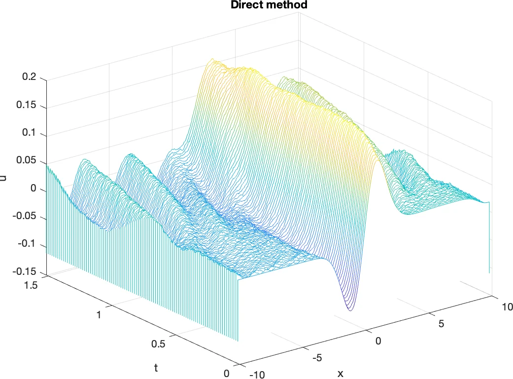
Restricting to the diagonal (y = z = 0) recovers the standard potential KdV equation ∂ₜu = μ∂ₓ³u − 3μ(∂ₓu)².

For non‑commutative extensions, the operators A and D are chosen as i f(P P†) and i h(∂ₓ) respectively, with f and h polynomial functions. This yields a non‑local nonlinear Schrödinger‑type equation for g:

i∂ₜg = h(∂ₓ)g + g ⋆ f ⋆ (g ⋆ g†),

where “⋆” denotes the big matrix product. Setting f(x)=x reproduces the non‑local nonlinear Schrödinger equation, demonstrating that the Grassmannian flow approach accommodates both commutative and non‑commutative integrable models.

In a companion paper, the authors extend the method to Smoluchowski coagulation equations with constant frequency kernels. By interpreting the convolution structure of the coagulation kernel within the Fredholm relation, they obtain a graph‑flow generalisation that captures additive and multiplicative frequency cases.

Beyond theory, the paper discusses computational implications. Grassmannian flows provide a natural coordinate chart on the infinite‑dimensional Grassmann manifold, allowing the representation of rapidly growing modes (e.g., far‑field exponential growth) in a numerically stable way. Prior work on large‑scale spectral methods and Maslov index computation has already leveraged such flows; the present framework broadens these applications to a wider class of nonlinear PDEs.

In summary, the authors demonstrate that many PDEs—ranging from classical integrable equations (KdV, nonlinear Schrödinger) to non‑commutative and coagulation models—can be recast as linear operator evolutions coupled with a linear Fredholm equation. This unifies the inverse scattering transform, Riccati‑type formulations, and modern Grassmannian geometry, offering both a deeper analytical understanding and a promising avenue for efficient numerical algorithms.