Global stabilization of multiple integrators by a bounded feedback with constraints on its successive derivatives

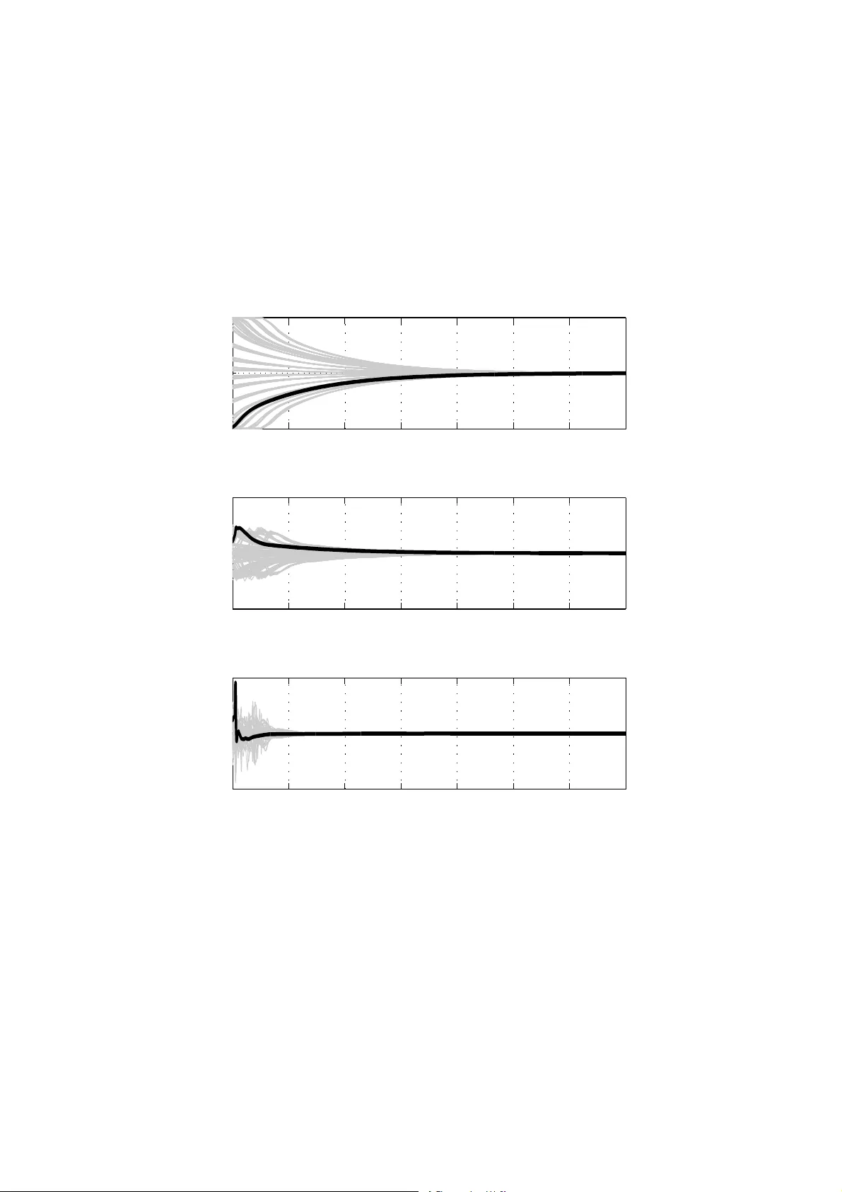
Global stabilization of multiple integrators by a bounded feedback with constraints on its successive d eriv atives Jonathan Laporte, Antoine Chaillet and Y acine Chitour ∗ † Abstract In this paper, we ad dress the global stabilizatio n o f cha ins of integrators by means of a bounded static feedbac k law whose p first time deri vati ves are bound ed. Our construction is based on the tech nique of ne sted satur ations introdu ced by T eel. W e show that the con trol am plitude and the maximum value of its p first deriv ati ves ca n be imposed below any pr escribed values. Our results ar e illustrated by the stabilization of the third ord er integrator on the feedback and its first two deriv ati ves. 1 Introd uction Actuator constraints is an important pract ical issue in control appl ications since it is a possibl e source of instability or performance degrada tion. Global stab ilizatio n of linear ti me-in v ariant (L TI) systems with actuator satu rations (o r b ounde d inpu ts) can be achie ved if and on ly the unc ontroll ed linear sy stem has no ei gen v alues with positi ve real part and is stabiliza ble [1]. Among tho se systems, chains of inte grators hav e recei ved specific atten tion. Saturatio n of a linear feedback is not globall y stabil izing as soon as the integra tor chain is of dimension great er than or equal to three [2, 3]. In [4] a globa lly stabi- lizing feedback is construct ed using nested saturat ions for the multiple integ rator . This con structi on has been e xtended to the general case i n [1], in wh ich a f am- ily of stabiliz ing fee dback laws is proposed as a linear combinati on of saturation functi ons. In [5] and [6], the issue of performance of these bounde d feedback s is in ves tigated for multiple integr ators and some improv ements are achie ved by us- ing v ariable le vels of saturat ion. A g ain sche duled feedb ack was p ropose d in [7 ] to ensure rob ustness to some classes of bo unded disturb ances. Global practica l stabi- lizatio n has been achiev ed in [8] in the presence of bounded actuato r disturbance s using a backst epping proce dure. ∗ This research was partiall y supported by a public grant overse en by the F rench ANR as part of the I n vestissements d’A venir program, through the iC ODE institute, research project funded by t he IDEX Paris-Saclay , ANR-11-IDEX-0003-02. † J. Laporte, A. Chaillet and Y . Chitour are with L 2S - Un iv . Paris Sud - Centrale- Sup ´ elec. 3, rue Joliot-Curie. 91192 - Gif sur Yvette, F rance. jonathan.lapor te, antoine.chai llet, yacine.chitour@l2s.cen tralesupelec.fr 1 T echnologica l consider ations may not only lead to a limited amplitude of the applie d control law , b ut also to a limited reacti vity . This problem is known as rate satura tion [9] and correspo nds to the situation when the si gnal deli vered by the ac- tuator cannot ha ve too fast v ariatio ns. T his issue has been addre ssed for instance in [10]-[11]. In [10, 12], regiona l stability is ensured through LMI-based conditions. In [9], a gain schedulin g techniq ue is used to ensu re semi-g lobal stabilization of in- teg rator chains. In [13], semi-glob al sta bilizati on is obtain ed vi a low-gain feedback or lo w-and-high-g ain feedback . In [11], a backsteppi ng procedure is propose d to global ly stabilize a nonline ar system with a control law whose amplitude and fi rst deri vati ve are bounded independen tly of the initial state. In this paper , we deepen the in vestiga tions on globa l stabilizat ion of L TI sys- tems subject to bounde d actuatio n with ra te con straints . W e consider rate con- straint s that affect only the first deri vati ve of the control signal, b ut also its succes- si ve p first deri v ati ves, where p denotes an arbitrary positi ve inte ger . Foc using on chains of integrat ors of arbitrary dimension , we propos e a static feedback law that global ly stabiliz es chains of integr ators, and whose magnitude and p first deri va- ti ves are below arbitrari ly prescrib ed va lues at all times. Our control law is based on the nested saturations introduced in [4]. W e rely on specific saturatio n fun ctions, which are linear in a neighborhoo d of the origin and constant for larg e val ues of their ar gument. This paper is or ganized as follo w s. In Section 2 , w e provide definitio ns and state our mai n result. The proof of th e main result is gi ven in Section 3 based on sev eral technical lemmas. In Section 4, we test the ef fi cienc y of the propo sed contro l la w via numerical simulati ons on the th ird o rder in tegr ator , with a fe edback whose magnitude and two first deriv ati ves are bounded by prescribed valu es. W e pro vide some conclusion s and possible future extens ions in Section 5. Notations. The functio n sign : R \{ 0 } → R is defined as sign ( r ) : = r / | r | . Giv en a set I ⊂ R and a constant a ∈ R , w e let I ≥ a : = { x ∈ I : x ≥ a } . Gi ven k ∈ N and m ∈ N ≥ 1 , we say that a functio n f : R m → R is of class C k ( R m , R ) if its dif ferentials up to order k exist and are continu ous, and we use f ( k ) to deno te the k -th order deri vati ve of f . By con vent ion, f ( 0 ) : = f . The facto rial of k is denote d by k !. W e define J m , k K : = { n ∈ N : n ∈ [ m , k ] } . W e use R m , m to denote the set of m × m matrice s w ith real coefficien ts. J m ∈ R m , m denote s the m -th Jordan block, i.e. the m × m matrix giv en by ( J m ) i , j = 1 if i = j − 1 and zero otherwise. For each i ∈ J 1 , m K , e i ∈ R m refers to the column vector with coordinate s equal to zero exc ept the i -th one equal to one. 2 Statement of the main result In this section we present our main result on the stabiliza tion of the multiple inte- grator s with a control law whose magnitude and p first deriv ativ es are bounded by prescr ibed constant s. Gi ven n ∈ N ≥ 1 , the multiple integrat or of length n is gi ven 2 by          ˙ x 1 = x 2 , . . . ˙ x n − 1 = x n , ˙ x n = u . (1) Letting x : = ( x 1 , . . . , x n ) , System (1) can be compactly written as ˙ x = J n x + e n u . In order to make the objecti ves of this paper more precise, we start by introd ucing the notion of p -bounded feedback law by ( R j ) 0 ≤ j ≤ p for System (1), which will be used all along the docu ment. Definition 1. Given n ∈ N ≥ 1 and p ∈ N , let ( R j ) 0 ≤ j ≤ p denote a family of positive consta nts. W e say that ν : R n → R is a p-boun ded feedba c k law by ( R j ) 0 ≤ j ≤ p for System (1) if, for every trajecto ry of the close d loop system ˙ x = J n x + e n ν ( x ) , the time functio n u : R ≥ 0 → R defined by u ( t ) = ν ( x ( t )) for all t ≥ 0 satisfies, for all j ∈ J 1 , p K , sup t ≥ 0 n    u ( j ) ( t )    o ≤ R j . Based on this definition, we can restate our stabiliz ation proble m as follo ws. Giv en p ∈ N and a set of positi ve real numbers ( R j ) 0 ≤ j ≤ p , our aim is to design a feedba ck la w ν which is a p -bou nded fe edback law by ( R j ) 0 ≤ j ≤ p for System (1) such that the o rigin of the closed-l oop syst em ˙ x = J n x + e n ν ( x ) is globa lly asympto tically stable. The case p = 0 corres ponds to global stabiliza tion with bound ed state feedba ck and has been addr essed in e.g. [4, 5, 6]. The case p = 1 corres ponds to global stabilizati on with bounded state feedback and limited rate, in the line of e.g. [10, 12, 9, 13, 11]. Inspir ed by [4], our design for an arbitrary order p is based on a nested saturations feedback, w here saturations belong to the follo wing class of functio ns. Definition 2. G iven p ∈ N , S ( p ) is defined as the set of all functions σ of class C p ( R , R ) , whic h ar e odd, and such that ther e e xists positive constants α , L, σ max and S satisfyin g, for all r ∈ R , (i) r σ ( r ) > 0 , w hen r 6 = 0 , (ii) σ ( r ) = α r, w hen | r | ≤ L, (iii) | σ ( r ) | = σ max , when | r | ≥ S . In the seque l, we associa te with eve ry σ ∈ S ( p ) the 4-tuple ( σ max , L , S , α ) . 3 The consta nts σ max , L , α , and S will be exten si vely used through out the paper . Figure 1 helps fixing the ideas. σ max repres ents the saturation lev el, m eaning the maximum v alue that can be reach ed by the sat uration . L denotes the linearity thresh old: for al l | r | ≤ L , the satura tion beha ves like a purely linear gain. α is the v alue of th is gain tha t is, the sl ope of the saturation in the linear region. S repres ents the saturati on threshold: for all | r | ≥ S , the function saturate s and takes a single va lue (either − σ max or σ max ). Notice that it necess arily holds that S ≥ L and the equality may only hold when p = 0. W e also stress that the succes si ve deri vati ves up to order p of an ele ment of S ( p ) are bounded . An exampl e of such functi on is gi ven in Section 4 for p = 2. Figure 1: A typic al e xample of a S ( p ) saturation function w ith const ants ( σ max , L , S , α ) . Based on these two definitions, we are no w ready to presen t our main result, which establis hes that global stabiliz ation on any chain of inte grators by boun ded feedba ck with constrain ed p first deriv ativ es can always be achiev ed by a particular choice of neste d saturations. Theor em 1. Given n ∈ N ≥ 1 and p ∈ N , let ( R j ) 0 ≤ j ≤ p be a family of positive con- stants . F or ev ery se t o f s atur ation funct ions σ 1 , . . . , σ n ∈ S ( p ) , the r e ex ists ve ctor s k 1 , . . . , k n in R n , and positive constants a 1 , . . . , a n suc h that the feedbac k law ν de- fined, for eac h x ∈ R n , as ν ( x ) = − a n σ n  k T n x + a n − 1 σ n − 1  k T n − 1 x + . . . + a 1 σ 1 ( k T 1 x )  . . .  (2) is a p-boun ded feedbac k la w by ( R j ) 0 ≤ j ≤ p for System (1), and the origin of the closed -loop system ˙ x = J n x + e T n ν ( x ) is globally asymptot ically stable . The proof of this result is giv en in Section 3. It prov ides a bov e th eorem w e gi ve belo w also provid es an expli cit choice of the gain ve ctors k 1 , . . . , k n and constan ts a 1 , . . . a n . 4 Remark 1. In [1], a stabili zing feedbac k law was constru cted using linear com- binati ons of saturat ed functio ns. That feedbac k with satura tion function s in S ( p ) canno t be a p-bou nded feedbac k for System (1). T o see this, consider the multi- inte grator of length 2 , given by ˙ x 1 = x 2 , ˙ x 2 = u. A ny stabi lizing feedbac k us- ing a linear combinati on of satur ation functions in S ( p ) is given by ν ( x 1 , x 2 ) = − a σ 1 ( bx 2 ) − c σ 2 ( d ( x 2 + x 1 )) , w her e the constants a, b, c, and d ar e chosen to in- sur e stability of the closed-l oop system accor ding to [1]. L et u ( t ) = ν ( x 1 ( t ) , x 2 ( t )) for all t ≥ 0 . A straightf orwar d computation yields ˙ u ( t ) = − ab σ ( 1 ) 1 ( ax 2 ( t )) u ( t ) − cd σ ( 1 ) 2 ( d ( x 2 ( t ) + x 1 ( t )))( x 2 ( t ) + u ( t )) . Now consider a solutio n with initial con- dition x 2 ( 0 ) = x 20 , and x 1 ( 0 ) = − x 20 suc h that σ ( 1 ) 1 ( ax 20 ) = 0 . W e then have ˙ u ( 0 ) = − cd σ ( 1 ) 2 ( 0 )( x 20 + u ( 0 )) , whose norm is gre ater than A ( | x 20 | − B ) for some positi ve constan ts A , B. Thus | ˙ u ( 0 ) | gr ows unboun ded as | x 20 | te nds to infinity , which c ontr adicts the definit ion of a p-bou nded feedbac k. Remark 2. Our construct ion is devel oped for chains of inte grator , but it may fai ls for a gener al linear system stabilizab le by bound ed inputs. Consider for instanc e the harmonic oscillator given by ˙ x 1 = x 2 , ˙ x 2 = − x 1 + u and a bound ed stabi lizing law given by u ( t ) = − σ ( x 2 ( t )) with σ ∈ S ( p ) for some inte ger p. The time deriva- tive of u ver ifies | ˙ u ( t ) | ≥   σ ( 1 ) ( x 2 ( t ))   ( | x 1 ( t ) | − | u ( t ) | ) , which gr ows unboun ded as the state norm incr eases, thus contradi cting the definiti on of p-bounded feedbac k. 3 Pr oof of the main result 3.1 T echnical lemma W e start by giv ing a lemma that provid es an upper bound of composed functio ns by expl oiting the saturatio n region of the functio ns in S ( p ) . Lemma 1. Given k ∈ N , let f and g be functions of class C k ( R ≥ 0 , R ) , σ be a satur ation functi on in S ( k ) with con stants ( α , L , S , σ max ), and E and F be subsets of R ≥ 0 suc h that E ⊆ F . Assume that | f ( t ) | > S , ∀ t ∈ F \ E , (3) and ther e exis ts positive consta nts M , Q 1 , . . . , Q k suc h that   f ( k 1 ) ( t )   ≤ Q k 1 , ∀ t ∈ E , ∀ k 1 ∈ J 1 , k K , (4)   g ( k ) ( t )   ≤ M , ∀ t ∈ F . (5) Then the k th-or der deriva tive of h : R ≥ 0 → R , defined by h ( · ) = g ( · ) + σ ( f ( · )) , satisfi es    h ( k ) ( t )    ≤ M + k ∑ a = 1 σ a B k , a ( Q 1 , . . . , Q k − a + 1 ) , ∀ t ∈ F , (6) 5 wher e B k , a ( Q 1 , . . . , Q k − a + 1 ) is a p olynomial functio n of Q 1 , . . . , Q k − a + 1 , and σ a : = max s ∈ R | σ ( a ) ( s ) | for each a ∈ J 1 , k K . Pr oof of Lemma 1. T he proo f relies on Fa ` a Di Bruno’ s formula, w hich we recall Lemma 2 (Fa ` a Di Brun o’ s formula, [14], p. 96) . Giv en k ∈ N , let φ ∈ C k ( R ≥ 0 , R ) and ρ ∈ C k ( R , R ) . Then the k -th or der deriv ative of the composi te function ρ ◦ φ is given by d k d t k ρ ( φ ( t )) = k ∑ a = 1 ρ ( a ) ( φ ( t )) B k , a  φ ( 1 ) ( t ) , . . . , φ ( k − a + 1 ) ( t )  , (7) wher e B k , a is the Bell polyn omial given by B k , a  φ ( 1 ) ( t ) , . . . , φ ( k − a + 1 ) ( t )  : = ∑ δ ∈ P k , a c δ k − a + 1 ∏ l = 1  φ ( l ) ( t )  δ l (8) wher e P k , a denote s the set of ( k − a + 1 ) − tup les δ : = ( δ 1 , δ 2 , . . . , δ k − a + 1 ) of posi- tive inte gers satisfying δ 1 + δ 2 + . . . + δ k − a + 1 = a , δ 1 + 2 δ 2 + . . . + ( k − a + 1 ) δ k − a + 1 = k , and c δ : = k ! /  δ 1 ! · · · δ k − a + 1 ! ( 1! ) δ 1 · · · (( k − a + 1 ) ! ) δ k − a + 1  . Using Lemma 2, a straig htforw ard computation yield h ( k ) ( t ) = g ( k ) ( t ) + k ∑ a = 1 σ ( a ) ( f ( t )) B k , a  f ( 1 ) ( t ) , . . . , f ( k − a + 1 ) ( t )  . Since σ ∈ S ( k ) , (3) ensures that the set F \ E is containe d in the saturat ion zone of σ . It follo ws that d k d t k σ ( f ( t )) = 0 , ∀ t ∈ F \ E . (9) Furthermor e, from (4) and (8) it holds that, for all t ∈ E ,    B k , a  f ( 1 ) ( t ) , . . . , f ( k − a + 1 ) ( t )     ≤ ∑ δ ∈ P k , a c δ k − a + 1 ∏ l = 1 Q δ l l , = B k , a ( Q 1 , . . . , Q k − a + 1 ) . From definition of σ a and (7), we get that     d k d t k σ ( f ( t ))     ≤ k ∑ a = 1 σ a B k , a ( Q 1 , . . . , Q k − a + 1 ) , ∀ t ∈ E . (10) In view of (9 ), the estimate (10) is v alid on the whole se t F . Thanks to (5), a straigh tforwa rd computation leads to the estimate (6). 6 3.2 Intermediate r esults In this subsect ion we pro vide two propos itions which will be used in the proof of Theorem 1. W e start by introduc ing some necess ary notatio n. Giv en n ∈ N ≥ 1 and p ∈ N , l et µ 1 , . . . , µ n be saturatio ns in S ( p ) with re specti ve consta nts ( µ max i , L µ i , S µ i , α µ i ) , i ∈ J 1 , n K . W e define, for each i ∈ J 1 , n K , µ i , j : = m ax n    µ ( j ) i ( r )    : r ∈ R o , ∀ j ∈ J 1 , p K , (11) b µ i : = m ax  | r − µ i ( r ) | : | r | ≤ S µ i + 2 µ max i − 1  . (12) W e also let b µ n : = max  µ n ( r ) r : 0 < | r | ≤ S µ n  , (13) b µ n : = min  µ n ( r ) r : 0 < | r | ≤ S µ n  . (14) Note that these quant ities are well defined since the functi ons µ i are all in S ( p ) . W e also m ake a linear change of coordi nates y = H x , with H ∈ R n , n , that puts System (1) into the form ˙ y i = α µ n n ∑ l = i + 1 y l + u , ∀ i ∈ J 1 , n K , (15) with the con vention n ∑ l = n + 1 = 0. The matrix H can be determin ed from y n − i = i ∑ k = 0 i ! k ! ( i − k ) !  α µ n  k x n − k , ∀ i ∈ J 0 , n − 1 K . (16) For this sys tem, we define a nested saturatio ns feedback law ϒ : R n → R as ϒ ( y ) = − µ n ( y n + µ n − 1 ( y n − 1 + . . . + µ 1 ( y 1 )) . . . ) . (17) Let y ( · ) be a trajec tory of the system ˙ y i = α µ n n ∑ l = i + 1 y l + ϒ ( y ) , ∀ i ∈ J 1 , n K , (18) which is the closed-loop system (15 ) w ith the feedba ck defined in (17). For each i ∈ J 1 , n K , the time function z i : R ≥ 0 → R is defined recursi vely as z i ( · ) : = y i ( · ) + µ i − 1 ( s i − 1 ( · )) , with µ 0 ( · ) = 0. N otice that with the abov e functions, the closed loop syste m (18) can be re written as    ˙ y i = α µ n z n − µ n ( z n ) + α µ n n − 1 ∑ l = i + 1 ( z l − µ l ( z l )) − α µ n µ i ( z i ) , ∀ i ∈ J 1 , n − 1 K , ˙ y n = − µ n ( z n ) . (19) 7 For i ∈ J 1 , n K , we also let E i : =  y ∈ R n : | y v | ≤ S µ v + µ max v − 1 , ∀ v ∈ J i , n K  , (20) with µ max 0 = 0, and I i : = { t ∈ R ≥ 0 : y ( t ) ∈ E i } . (21) Note that from t he definitions of I i and E i , we hav e I 1 ⊆ I 2 ⊆ . . . ⊆ I n , and a straight- forwar d computation yields | z i ( t ) | > S µ i , ∀ t ∈ I i + 1 \ I i , ∀ i ∈ J 1 , n − 1 K , (22) | z n ( t ) | > S µ n , ∀ t ∈ R ≥ 0 \ I n , (23) which allo ws us to determine when s aturatio n occurs. Moreove r fro m the d efi- nition s of saturat ion functions of class S ( p ) , E i , I i , (13) and (14), the follo wing estimates can easily be deri ved: | z i ( t ) − µ i ( z i ( t )) | ≤ b µ i , ∀ t ∈ I i , (24)   α µ n z n ( t ) − µ n ( z n ( t ))   ≤ ( b µ n − B µ n )( S µ n + 2 µ max n − 1 ) , ∀ t ∈ I n , (25) with B µ n : = m in n b µ n , µ max n S µ n + 2 µ max n − 1 o . The follo wing statement pro vides e xplicit bounds o n the successi ve deri va ti ves of eac h func tions y i ( t ) , z i ( t ) for ea ch i ∈ J 1 , n K and the time fun ction gi ven by u ( · ) = ϒ ( y ( · )) . Pro position 1. Given n ∈ N ≥ 1 and p ∈ N , let µ 1 , . . . , µ n be satur ation function s in S ( p ) w ith re spectiv e constan ts ( µ max i , L µ i , S µ i , α µ i ) for eac h i ∈ J 1 , n K . W ith the notation intr oduced in this section and the B ell polyno mials intr oduced in (8) , eve ry trajecto ry of the closed-loop s ystem (18) satisfies, f or each i ∈ J 1 , n K and each j ∈ J 1 , p K , ( P 1 ( i , j )) :    y ( j ) i ( t )    ≤ Y i , j , ∀ t ∈ I i ; (26) ( P 2 ( i , j )) :    z ( j ) i ( t )    ≤ Z i , j , ∀ t ∈ I i ; (27) ( P 3 ( j )) : sup t ≥ 0 n    u ( j ) ( t )    o ≤ j ∑ q = 1 G q , j µ n , q ; (28) wher e Y i , j , Z i , j , and G q , j ar e independent of initial con dition s and ar e obt ained r ecursiv ely as follows: for j = 1 , Y n , 1 : = µ max n , Y i , 1 : = ( b µ n − B µ n )( S µ n + 2 µ max n − 1 ) + α µ n n − 1 ∑ l = i + 1 b µ l + α µ n µ max i , ∀ i ∈ J 1 , n − 1 K , Z 1 , 1 : = Y 1 , 1 , Z i , 1 : = Y i , 1 + µ i − 1 , j Z i − 1 , 1 , ∀ i ∈ J 2 , n K , G 1 , 1 : = Z n , 1 8 and, for each j ∈ J 2 , p K , Y i , j : = α µ n n ∑ b = i + 1 Y b , j − 1 + j − 1 ∑ q = 1 G q , j − 1 µ n , q , ∀ i ∈ J 1 , n − 1 K , Z 1 , j : = Y 1 , j , Z i , j : = Y i , j + j ∑ a = 1 µ i − 1 , a B j , a ( Z i − 1 , 1 , . . . , Z i − 1 , j − 1 + a ) , ∀ i ∈ J 2 , n K , G q , j : = B j , q ( Z n , 1 , . . . , Z n , j − q + 1 ) , ∀ q ∈ J 1 , j K . Pr oof of Pr oposition 1. Let y ( t ) be a trajec tory of the closed loo p s ystem (18). The right-h and side of (18) being of class C p ( R n , R n ) and globally Lipschitz, System (18) is forward comple te and its tr ajectori es are of class C p + 1 ( R ≥ 0 , R n ) . T herefo re the succes si ve time deriv ati ves of y i ( t ) , z i ( t ) , and u ( t ) are well defined. W e es tablish the re sult by induction on j . W e star t by j = 1. W e begin to prov e that P 1 ( i , 1 ) holds for all i ∈ J 1 , n K . Let i ∈ J 1 , n − 1 K . From (19), (24), and (25) a straigh tforwa rd computation leads to | ˙ y i ( t ) | ≤ ( b µ n − B µ n )( S µ n + 2 µ max n − 1 ) + c n − 1 ∑ l = i + 1 b µ l + c µ max i , for a ll t ∈ I i + 1 . Since I i ⊆ I i + 1 , th e abo ve estima te is sti ll true on I i . Moreo ver , from (19) it holds that | ˙ y n ( t ) | ≤ µ max n at all positi ve times. P 1 ( i , 1 ) has been prov en for each i ∈ J 1 , n K . W e no w prove by induction on i the statement P 2 ( i , 1 ) . Since z 1 ( · ) = y 1 ( · ) , the case i = 1 is done. Assume that, for a giv en i ∈ J 1 , n − 1 K , the state ment P 2 ( i 2 , 1 ) holds for all i 2 ≤ i . From Lemm a 1 (with k = 1, f = z i , g = y i + 1 , h = z i + 1 , σ = µ i , Q 1 = Z i , 1 , M = Y i + 1 , 1 , σ 1 = µ i , 1 , E = I i , F = I i + 1 , and (22 )), we can establ ish that P 2 ( i + 1 , 1 ) holds. Thus P 2 ( i , 1 ) holds for all i ∈ J 1 , n K . Notice that u ( · ) = − µ n ( z n ( · )) . W e then can establ ish P 3 ( 1 ) from Lemma 1 (with k = 1, f = z n , g ≡ 0, h = u , σ = µ n , Q 1 = Z 1 , i , M = 0, σ 1 = µ n , 1 , E = I n , F = R ≥ 0 and (23)). This ends the case j = 1. Assume that fo r a gi ven j ∈ J 1 , p − 1 K , statemen ts P 1 ( i , j 2 ) , P 2 ( i , j 2 ) and P 3 ( j 2 ) hold for all j 2 ≤ j and all i ∈ J 1 , n K . Let i ∈ J 1 , n K . From (15), a straightf orward computa tion yields    y ( j + 1 ) i ( t )    ≤ α µ n n ∑ l = i + 1    y ( j ) l ( t )    +    u ( j ) ( t )    , ∀ t ≥ 0 . From P 3 ( j ) , P 1 ( i + 1 , j ) , . . . , P 1 ( n , j ) , we obtain that    y ( j + 1 ) i ( t )    ≤ α µ n n ∑ l = i + 1 Y l , j + j ∑ q = 1 G q , j µ n , q , ∀ t ≥ I i . 9 Thus the stateme nt P 1 ( j + 1 , i ) is prov en for all i ∈ J 1 , n K . W e now prove by inducti on on i the statement P 2 ( i , j + 1 ) . As before, since z 1 = y 1 , the case for i = 1 is done. Assume that fo r a gi ven i ∈ J 1 , n − 1 K , the statemen t P 2 ( i 1 , j + 1 ) holds for all i 1 ≤ i . From L emma 1 (with k = j + 1, f = z i , g = y i + 1 , h = z i + 1 , σ = µ i , Q k 1 = Z i , k 1 , M = Y i + 1 , j + 1 , σ a = µ i , a , E = I i , F = I i + 1 , and (22)), w e can establish that P 2 ( i + 1 , j + 1 ) holds. P 2 ( i , j + 1 ) is thus satisfied for all i ∈ J 1 , n K . Finally , we can estab lish P 3 ( j + 1 ) from Lemm a 1 (with k = j + 1, f = z n , g ≡ 0, h = u , σ = µ n , Q k 1 = Z n , k 1 , M = 0, σ a = µ n , a , E = I n , F = R ≥ 0 and (23)). This ends the proo f of Propositio n 1. W e ne xt provi de suf ficient conditi ons on the para meters of the satura tion func- tions in S ( p ) guarante eing global asympto tic stability of the closed-loo p system (18). Pro position 2. Given n ∈ N and p ∈ N , let µ 1 , . . . , µ n be saturat ion functions in S ( p ) with r espective constant s ( µ max i , l l µ i , l s µ i , α µ i ) for each i ∈ J 1 , n K and assume that, for all i ∈ J 1 , n − 1 K , α µ i = 1 , (29a) µ max i < L µ i + 1 / 2 . (29b) Then the origi n of the closed- loop system (18) is globa lly asymptot ically stable . Actually the abov e proposition is almost the same as the one gi ven in [4], ex- cept that we allow the first lev el of saturation µ n to ha ve a slope diff erent from 1. Pr oof of Pr oposition 2. W e prov e that after a finite time any trajectory of the closed- loop system (18) ente rs a regio n in which t he fee dback (1 7) becomes simply linear . T o that end, we consider the L yapunov function candidate V n : = 1 2 y 2 n . Its deriv a- ti ve al ong the trajectorie s of (18) reads ˙ V n = − y n µ n ( y n + µ n − 1 ( z n − 1 )) . From (29b), we can obtain that for all | y n | ≥ L µ n / 2 ˙ V n ≤ − θ L µ n / 2 , (30) where θ = inf r ∈ [ L µ n / 2 − µ n − 1 , S µ n ] { µ n ( r ) } . W e next sho w that there exists a time T 1 ≥ 0 such that | y n ( t ) | ≤ L µ n / 2, for all t ≥ T 1 . T o prov e that we hav e the follo wing alternati ves : either for ev ery t ≥ 0, | y n ( t ) | ≤ L µ n / 2 and we are done, or there exi st T 0 ≥ 0 such that | y n ( T 0 ) | > L µ n / 2. 10 In that case ther e ex ists ˜ T 0 ≥ T 0 such tha t y n ( ˜ T 0 ) = L µ n / 2 (otherwise thanks to (30), V n ( t ) → − ∞ as t → ∞ which is impossib le). D ue to (30), w e hav e | y n ( t ) | < L µ n / 2 in a right open neighb ourhoo d of ˜ T 0 . Suppose that there exis ts a positi ve time ˜ T 1 > ˜ T 0 such that   y n ( ˜ T 1 )   ≥ L µ n / 2. T hen by continui ty , there mus t exists ˜ T 2 ∈ ( ˜ T 0 , ˜ T 1 ] such that   y n ( ˜ T 2 )   = L µ n / 2, and | y n ( t ) | < L µ n / 2 for all t ∈ ( ˜ T 0 , ˜ T 2 ) . Ho wev er , it then follo ws from (30) that for a left open neighbour hood of ˜ T 2 we ha ve | y n ( t ) | >   y n ( ˜ T 2 )   = L µ n / 2. This i s a contradicti on with t he fac t that o n a right open neighbo urhoo d of ˜ T 0 w ha ve | y n ( t ) | < L µ n / 2. Therefore, for ev ery ˜ T 1 > ˜ T 0 , one has   y n ( ˜ T 1 )   < L µ n / 2 and the claim is prov ed. It follo ws from (29b) that | y n ( t ) + µ n − 1 ( z n − 1 ( t )) | ≤ L µ n , ∀ t ≥ T 1 . Therefore µ n operat es in its lin ear regio n after time T 1 . Similarly , we no w conside r V n − 1 : = 1 2 y 2 n − 1 , whose deri vat iv e along the trajectorie s of (18) satisfies ˙ V n = − α µ n y n − 1 µ n − 1  y n − 1 + µ n − 2 ( y n − 2 + . . . )  , ∀ t ≥ T 1 . Reasonin g as b efore and in v oking (29b), there exists a time T 2 > 0 such that | y n − 1 ( t ) | ≤ L µ n − 1 / 2 and µ n − 1 operat es in its linear reg ion for all t ≥ T 2 . By repea ting this procedu re, we co nstruct a time T n such that for all times greate r than T n the whole feedbac k law be comes linear . T hat is ϒ ( y ( t )) = − α µ n ( y n ( t ) + . . . + y 1 ( t )) , for all t ≥ T n . System (18 ) becomes simply linear and its loca l e xponen tial stabilit y follo ws readily . Thus the origin of S ystem (18) is globally asympto tically stable , which conclu des the proof of Proposit ion 2. 3.3 Pr oof of Theor em 1 W e now proceed to the proof of T heorem 1 by expli citly construc ting the vector s k 1 , . . . , k n and the constants a 1 , . . . , a n . This proof can thus be used as an algorith m to comput e the nested feedba ck propos ed in Theorem 1. Giv en p ∈ N and n ∈ N ≥ 1 , let σ i be saturatio n functio ns in S ( p ) with constants ( σ max i , L σ i , S σ i , α σ i ) for each i ∈ J 1 , n K , and let ( R j ) 0 ≤ j ≤ p be a family of positi ve 11 consta nts. W e let R : = m in { R j : j ∈ J 1 , p K } , σ n , j : = m ax r ∈ R n    σ ( j ) n ( r )    o , ∀ j ∈ J 1 , p K , α ˜ µ : = R 0 L σ n α σ n / σ max n , ˜ µ n , j : = R 0 σ n , j ( L σ n ) j σ max n , ∀ j ∈ J 1 , p K , b σ n : = m ax  σ n ( r ) r : 0 < | r | ≤ S σ n  , b σ n : = m in  σ n ( r ) r : 0 < | r | ≤ S σ n  . Note that all these quantities are well defined since σ n ∈ S ( p ) . W e first constr uct satura tions µ 1 , . . . µ n in order to use result s in Section 3.2. Let ( µ max i ) 1 ≤ i ≤ n − 1 and ( L µ i ) 1 ≤ i ≤ n − 1 be two sets of po siti ve consta nts such that µ max n − 1 < 1 2 , L µ n − 1 = µ max n − 1 L σ n − 1 α σ n − 1 σ max n − 1 , (31) and, for each i ∈ J 1 , n − 2 K , µ max i < 1 2 L µ i + 1 , L µ i = µ max i L σ i α σ i σ max i . (32) For each i ∈ J 1 , n − 1 K , the satura tion functio n µ i ∈ S ( p ) with consta nts ( µ max i , L µ i , S µ i , 1), where S µ i = S σ i L µ i / L σ i , is then gi ven by µ i ( s ) : = µ max i σ max i σ i  s L σ i L µ i  , ∀ s ∈ R . For λ ≥ 1, to be chosen later , w e define the satur ation function µ n ∈ S ( p ) , with consta nts µ max n = R 0 , L µ n = λ , S µ n = S σ n λ / L σ n , and α µ n = α ˜ µ / λ , by µ n ( s ) : = R 0 σ max n σ n  s L σ n λ  , ∀ s ∈ R . From (3 1) an d (32) we can establish that the functi ons µ 1 , . . . , µ n satisfy condi- tions (29). It foll o ws from Proposit ion 2 that the nested feedbac k law ϒ ( y ) defined in (17) stabiliz es globall y asymptotically the origin of (15). W e ne xt choose λ in such a w ay that ϒ ( y ) is a p -boun ded feedback law by 12 ( R j ) 0 ≤ j ≤ p for System (15). T o that end, first notice that b µ n = α ˜ µ b σ n λ α σ n , (33) b µ n = α ˜ µ b σ n λ α σ n , (34) B µ n = 1 λ min  α ˜ µ b σ n α σ n , R 0 S σ n / L σ n + 2 σ max n − 1 / λ  , (35) µ n , q = ˜ µ n , q / λ q , (36) where b µ n , b µ n , and µ n , q are defined in (13), (14), an d (11) respec ti vely . Using Proposit ion 1, it fol lo ws that ev ery trajectory of the closed -loop syste m (18) satis- fies, for each j ∈ J 1 , p K , sup t ≥ 0 n    u ( j ) ( t )    o ≤ j ∑ q = 1 G q , j ˜ µ n , q λ q . (37) By substituti ng (33), (34), (35), and (36) into the recursion in P roposi tion 1, it can be seen that, for each j ∈ J 1 , p K , j ∑ q = 1 G q , j ˜ µ n , q λ q = 1 λ P ( 1 λ ) where P is a polynomial with posit i ve coef fi cients. This sum is thus decreasin g in λ . Hence, we can pick λ ≥ 1 in such a way tha t j ∑ q = 1 G q , j ˜ µ n , q λ q ≤ R , ∀ j ∈ J 1 , p K . It follo ws that, for each j ∈ J 1 , p K , sup t ≥ 0 n    u ( j ) ( t )    o ≤ R ≤ R j . Recalling that the feedback ϒ is bounded by R 0 , we conclu de that it is p -bounded feedba ck law b y ( R j ) 0 ≤ j ≤ p for System (15). W ith the linear chang e y = H x , th e closed-lo op system (18) can be pu t into the form of the closed-loo p system (1) with u = ϒ ( H x ) . T hus, the sough t feedb ack law ν of Theorem 1 is obtained by ν ( x ) = ϒ ( H x ) . This leads to the follo wing choices of paramet ers: a n = R 0 / σ max n , a i = L σ i + 1 µ max i L µ i + 1 σ max i , ∀ i ∈ J 1 , n − 1 K , k T n x = L σ n L µ n x n , k T n − i x = L σ n − i L µ n − i i ∑ k = 0 i ! k ! ( i − k ) !  α ˜ µ L µ n  k x n − k , ∀ i ∈ J 1 , n − 1 K , and L µ n = λ . 13 4 Simulation In this sectio n, w e illustrate the applicabilit y and the performanc e of the proposed feedba ck on a particular exa mple. W e use the proced ure described in Section 3.3 in order to compute a 2-bound ed feedback law by ( 2 , 20 , 18 ) for the multiple inte- grator of leng th three. Our set of saturation functions is σ 1 = σ 2 = σ 3 = σ where σ is an S ( 2 ) saturation function with constants ( 2 , 1 , 2 , 1 ) giv en by σ ( r ) : =        r if | r | ≤ 1 , h 1 ( r ) if 1 ≤ | r | ≤ 1 . 5 , h 2 ( r ) if 1 . 5 ≤ | r | ≤ 2 , 2sign ( r ) otherwis e, with h 1 and h 2 were picke d in order to ensure sufficien t smoothness for σ : h 1 ( r ) : = sign ( r )( − 4 + 15 | r | − 18 r 2 + 10 | r | 3 − 2 r 4 ) , h 2 ( r ) : = 2sign ( r )( 25 − 60 | r | + 54 r 2 − 21 | r | 3 + 3 r 4 ) . In accordance with (31 ) and (32), we ch oose µ max 2 = 2 / 5, L µ 2 = 1 / 5, µ max 1 = 1 / 12, and L µ 1 = 1 / 24. Follo wing the procedure , we obtain that sup t ≥ 0 n    u ( 1 ) ( t )    o ≤ ( 7 . 91 + 4 . 3 5 λ ) / λ 2 , sup t ≥ 0 n    u ( 2 ) ( t )    o ≤ 26 . 2 λ 3 + 396 λ 2 + 1147 . 2 λ + 125 . 2 λ 4 . Choosin g λ = 6 . 5, we obtain that sup t ≥ 0    u ( 1 ) ( t )    ≤ 0 . 9, and sup t ≥ 0    u ( 2 ) ( t )    ≤ 18. The desire d feedback is then gi ven by ν ( x ) = − σ  1 6 . 5  x 3 + 1 5 σ  5 ( x 2 / 6 . 5 + x 3 + 1 24 σ  24 ( x 3 + 2 x 2 / 6 . 5 + x 1 / 6 . 5 2 ))   . This feedback law was tested in simulations. The results are present ed In Fig- ure 2. Tr ajector ies of the multiples integ rator of length 3 with the abov e feedback are plotted in grey for sev eral initial conditions . The correspon ding va lues of the contro l law and its time d eri v ati ves up to order 2 are shown i n Fig ure 3 . These grey curv es v alidate the fact that asymptot ic stability is reached an d that the con trol feedba ck magnitude, and two first deri v ati ves, nev er overp ass the prescribe d v al- ues ( 2 , 20 , 18 ) . In order to illus trate the beha viour of one particul ar trajec tory , the specific simulatio ns obtaine d for initia l conditi on x 10 = 446 . 7 937, x 20 = − 69 . 87 5 and x 30 = 11 . 05 are highl ighted in bold black. It can be seen from Figure 3 that our procedur e shows some conserv ativ eness the amplitude of the second deriv ati ve of the feedb ack nev er exceed s the value 2, althou gh maximum v alue of 18 was tole rated. 14 0 5 10 15 20 25 30 35 −1000 0 1000 Time x 1 (t) 0 5 10 15 20 25 30 35 −200 0 200 Time x 2 (t) 0 5 10 15 20 25 30 35 −20 0 20 Time x 3 (t) Figure 2: Evo lution of the states for a set of initial conditions . 15 0 5 10 15 20 25 30 35 −2 0 2 Time u(t) 0 5 10 15 20 25 30 35 −1 0 1 Time u (1) (t) 0 5 10 15 20 25 30 35 −2 0 2 Time u (2) (t) Figure 3: E v olution of the control and its deri vati ve up to order 2 for the same set of initia l conditions. 16 5 Conclusion W e hav e sho wn that any chain of integrato rs can be globally asymptotically stabi- lized by a static feedback whose magnitude and p first time deri v ati ves are below arbitra ry presc ribed v alues, unifo rmly with respect to all trajectorie s of the closed loop system. The design of this feedback relies on the techniq ue of nested satu- ration s first introduce d in [4]. The applicabil ity of the design proce dure and the perfor mance of the resultin g closed-loop syste m was tested on a particular exam- ple. The follo wing two problems can be consid ered for future works: i ) extendin g this res ult from inte grator chains to genera l linear systems stabili zable by boun ded input; ii ) designing a C ∞ bound ed feedback , all the s uccessi ve deri vati ves of whic h stand belo w prescr ibed constan ts at all times. Refer ences [1] H . J. Sussmann, E. D. S ontag , and Y . Y ang, “ A general result on the stabi- lizatio n of linear systems using bounded controls , ” Automatic Contr ol, IEEE T rans action s on , vo l. 39, pp. 2411–2425 , 1994. [2] A . T . Fuller , “In-the -lar ge stab ility of relay and saturat ing contr ol systems with linear control lers, ” Internatio nal Jou rnal of C ontr ol , v ol. 10, no. 4, pp. 457–4 80, 1969. [3] H . Sussmann and Y . Y ang, “On the stabil izabilit y of multiple integrat ors by means of bounde d feedback controls , ” in Decision and Contr ol, IEEE Con- fer ence on , Dec 1991, pp. 70–72 vol.1. [4] A . R. T eel, “Global stabiliz ation and restric ted tracking for multiple inte gra- tors with bounded control s, ” Systems and Contr ol Letters , vol. 18, no. 3, pp. 165 – 171, 1992. [5] N . Marchan d, “Further results on global stabilizati on for multiple inte grator s with bound ed contro ls, ” in Decisio n and Contr ol, IEEE Con fer ence on , 2003. [6] N . Marc hand and A. Hably , “Global stabi lizatio n of multip le integra tors with bound ed controls, ” Auto matica , vol. 41, no. 12, pp. 2147–2152 , 2005, hal- 00396 331. [7] A . Megrets ki, “Bibo output feedback stabil ization w ith satura ted control, ” in In IF AC W orld Congr ess , 1996, pp. 435–440. [8] S . Gayaka an d B. Y ao, “Globa l stabilizati on of a chain of integrato rs with input saturation and disturb ances, ” in American Contr ol Confer ence , 2011, pp. 3784 –3789. 17 [9] T . Lauvdal, R. Murray , and T . Fosse n, “Stabilizatio n of integ rator chains in the presen ce of magnitude and rate saturations : a gain schedulin g approach, ” in Decisio n and Contr ol, IEEE Confer ence on , vol . 4, Dec 1997, pp. 4004– 4005 v ol.4. [10] J. Gomes da Silva, J.M., S. T arbouriec h, and G. Garcia, “Local stabili zation of linear systems under amplitude and rate saturating actuato rs, ” A utomatic Contr ol, IEEE T ransa ctions on , vol. 48, no. 5, pp. 842– 847, May 2003 . [11] R. Freeman and L. Praly , “Integ rator backstepp ing for bounded controls and contro l rates, ” Automati c Contr ol, IEEE T ran saction s on , v ol. 43, no. 2, pp. 258–2 62, 1998. [12] S. Galeani, S . Onori, A. T eel, and L. Zaccarian, “ A magnitud e and rate sat- uratio n mode l and its use in the solution of a static anti-win dup pr oblem, ” Systems and Contr ol Letters , v ol. 57, no. 1, pp. 1 – 9, 2008. [13] A. Saberi, A. S toorv ogel, and P . Sannuti, Internal and E xterna l Stabiliz ation of Linear Systems with Constr aints , ser . Systems & C ontrol : Foundat ions & Applicat ions. Birkh ¨ auser Boston, 2012. [14] M. Haze winkel, Encyclo paedia of Mathematics (1) , ser . Encyclo paedia of Mathematic s: An Updated and Annotated T ranslati on of the S ov iet ”Mathe- matical Ency clopaed ia”. Springer , 1987. 18