mBART: Multidimensional Monotone BART

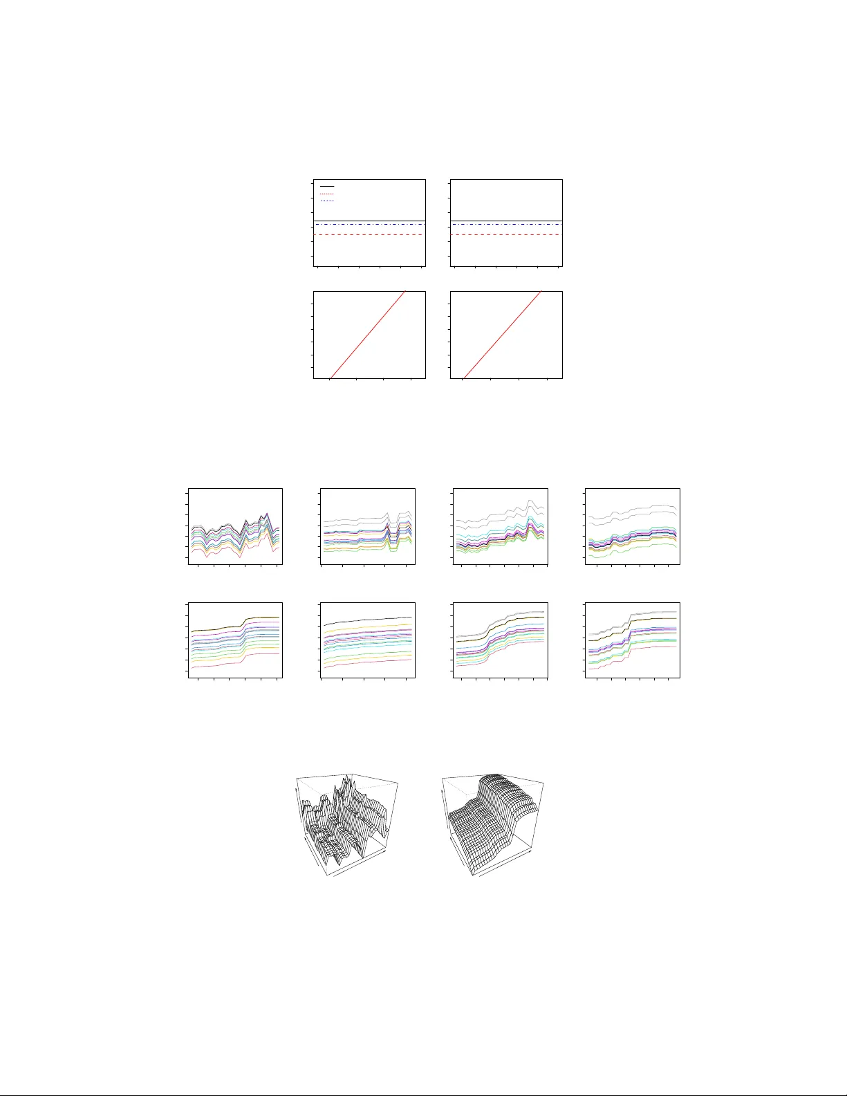
Ba y esian Analysis (0000) 00 , Num b er 0, pp. 1 mBART: Multidimensional Monotone BART Hugh A. Chipman ∗ , Edward I. George † , Rob ert E. McCullo c h ‡ and Thomas S. Shively . § Abstract. F or the disco v ery of regression relationships betw een Y and a large set of p p otential predictors x 1 , . . . , x p , the ﬂexible nonparametric nature of BAR T (Ba y esian Additive Regression T rees) allo ws for a muc h richer set of p ossibilities than restrictiv e parametric approaches. How ev er, sub ject matter considerations sometimes w arran t a minimal assumption of monotonicit y in at least some of the predictors. F or such contexts, we in tro duce mBAR T, a constrained version of BAR T that can ﬂexibly incorp orate monotonicity in an y predesignated subset of predictors using a multiv ariate basis of monotone trees, while av oiding the further conﬁnes of a full parametric form. F or such monotone relationships, mBAR T pro vides (i) function estimates that are smo other and more interpretable, (ii) b etter out-of-sample predictiv e performance, and (iii) less p ost-data uncertain ty . While many key asp ects of the unconstrained BAR T mo del carry ov er directly to mBAR T, the introduction of monotonicity constrain ts necessitates a fundamental rethinking of how the mo del is implemented. In particular, the original BAR T Mark o v Chain Mon te Carlo algorithm relied on a conditional conjugacy that is no longer av ailable in a monotonically constrained space. V arious simulated and real examples demonstrate the wide ranging p otential of mBAR T. MSC2020 subject classiﬁcations : Primary 62F15; secondary 62G08. Keyw o rds: Bay esian nonparametrics, ensemble mo del, isotonic regression, MCMC algorithm, m ultidimensional nonparametric regression, shap e constrained inference. 1 Intro duction Supp ose one w ould lik e to learn how Y dep ends on a v ector of p oten tial predictors x = ( x 1 , . . . , x p ) when no information is av ailable ab out the form of the relationship. In the absence of suc h prior information, the Ba yesian nonparametric approac h BAR T (Ba y esian Additive Regression T rees) can quickly disco v er the nature of this relation- ship; see Chipman, George, and McCullo ch (2010), hereafter CGM10. More precisely , based only on the assumption that Y = f ( x ) + ,  ∼ N (0 , σ 2 ) , (1.1) arXiv: 2010.00000 ∗ Department of Mathematics and Statistics, Acadia Universit y , Nov a Scotia, Canada hugh.c hipman@acadiau.ca † Department of Statistics, The Wharton School, University of Pennsylv ania, Philadelphia, P A, U.S.A. edgeorge@upenn.edu ‡ The School of Mathematical and Statistical Sciences, Arizona State Univ ersity , T emp e, AZ, U.S.A. robert.mccullo ch@asu.edu § Department of Information, Risk, and Op erations Management, Univ ersity of T exas at Austin, Austin, TX, U.S.A. T om.Shively@mccom bs.utexas.edu © 0000 International So ciet y for Bay esian Analysis DOI: 0000 2 mBAR T: Multidimensional Monotone BAR T BAR T can quickly obtain full p osterior inference for the unkno wn regression function, f ( x ) = E ( Y | x ) (1.2) and the unkno wn v ariance σ 2 . BAR T also pro vides predictiv e inference as w ell as model- free v ariable selection and in teraction detection, see Chipman, George, and McCulloch (2013), Bleich et al. (2014), and Kap elner and Bleich (2016). F requentist theoretical supp ort for the attractive empirical performance of BAR T has been recently developed in Ro c k o v a and v an der Pas (2020) and Ro ck ov a and Saha (2019), and for a k ernel- smo othed v ariant of BAR T in Linero and Y ang (2018). F or an excellent ov erview of BAR T and many of its recent related developmen ts, see Hill, Linero and Murray (2020) and the references therein. While the assumption free nature of BAR T is particularly v aluable when a trustable parametric form is una v ailable, sub ject matter considerations sometimes w arran t a min- imal prior assumption of monotonicity in at least some of the predictors in x . F or ex- ample, in one of our subsequent illustrative data sets, Y is the price of a used car and the x predictors include its age and mileage. All other things b eing equal, a prior as- sumption here that older cars as w ell as higher mileage cars sell for less on av erage, is comp elling. Man y other contexts where such prior monotonicity assumptions arise naturally , such as dose-resp onse function estimation in epidemiology or mark et demand function estimation in economics, can b e found in the references b elo w. T o harness such monotonicit y information, the main goal of this pap er is the in tro duction of monotone BAR T (hereafter mBAR T), a constrained v ersion of BAR T that restricts attention to regression functions f that are monotone in an y predesignated subset of the comp onen ts of x , while leaving the remaining comp onents unconstrained. In the now ric h literature on monotone function estimation, also known as isotonic regression, a wide v ariety of approac hes hav e b een proposed and applied b oth from the frequen tist and Ba y esian p oints of view. Including constrained nonparametric maximum lik eliho o d, spline mo deling, Gaussian pro cesses and pro jection-based metho ds among others, see for example, Barlow et. al. (1972), Mammen (1991), Lavine and Mo ckus (1995), Ramsay (1998), Holmes and Heard (2003), Neelon and Dunson (2004), Kong and Eubank (2006), Cai and Dunson (2007), Chernozhuk ov, F ernandez-V al and Gali- c hon (2009), Shiv ely , Sager and W alk er (2009), Meyer, Hackstadt and Hoeting (2011), Shiv ely , W alker and Damien (2011), Saarela and Arjas (2011), Lin and Dunson (2014), Chen and Samw orth (2016), W ang and Berger (2016), Lenk and Choi (2017), W ang and W elch (2018), Lin, St.Thomas, Piegorsch, Scott and Carv alho (2019), W estling, v an der Laan and Carone (2020) and the many references therein. In contrast to all these approaches, mBAR T is built on an easily constrained sum-of-trees approximation of f , comp osed of simple multiv ariate basis elements that can adaptively incorp orate n umerous predictors as well as their interactions. Inheriting the attractive prop erties of BAR T, mBAR T can quickly detect low dimensional signals in high dimensional re- gression settings with a rapidly mixing MCMC implemen tation that generates fully Ba y esian uncertaint y quan tiﬁcation as its output. The extension of BAR T to our monotonically constrained setting essentially requires t w o basic innov ations. First, it is necessary to develop general constraints for regression Chipman et al. 3 tree functions to b e monotone in any predesignated set of co ordinates. Under these constrain ts, the monotonicity of the full sum-of-trees approximation follows directly . The second inno v ation requires a new approac h for MCMC p osterior computation. Whereas the original BAR T form ulation allow ed straightforw ard marginalization o v er regression tree parameters exploiting conditionally conjugate priors, the constrained trees form ulation requires a more nuanced approac h because complete conjugacy is no longer av ailable. The outline of the pap er is as follo ws. In Section 2, we describ e in detail the con- strained sum-of-trees mo del used for monotone function estimation. Section 3 discusses the regularization prior for the trees while section 4 describ es the new MCMC algorithm required to implemen t mBAR T. Section 5 provides three simulated and tw o real data examples which illustrate the p otential inferen tial improv ements that mBAR T oﬀers. Section 6 con tains some concluding discussion. 2 A Monotone Sum-of-T rees Mo del The essence of BAR T is a sum-of-trees mo del appro ximation of the relationship b etw een y and x in ( 1.1 ); Y = m X j =1 g ( x ; T j , M j ) + ,  ∼ N (0 , σ 2 ) , (2.1) where each T j is a binary regression tree with a set M j of asso ciated terminal no de constan ts µ ij , and g ( x ; T j , M j ) is the function which assigns µ ij ∈ M j to x according to the sequence of decision rules in T j . These decision rules are binary partitions of the predictor space of the form { x ≤ a } vs { x > a } where the splitting v alue a is in the range of x . (A clarifying example of how g works appears in Figure 1 b elow and is describ ed later in this section). When m = 1, ( 2.1 ) reduces to the single tree model used by Chipman et al. (1998) for Ba yesian CAR T. Under ( 2.1 ), E ( Y | x ) is the sum, ov er trees T 1 , . . . , T m , of all the terminal no de µ ij ’s assigned to x by the g ( x ; T j , M j )’s. As the µ ij can take any v alues it is easy to see that the sum-of-trees mo del ( 2.1 ) is a ﬂexible representation capable of represen ting a wide class of functions from R n to R , especially when the num b er of trees m is large. Com- p osed of simple functions from R p to R , namely the g ( x ; T j , M j ), the multiv ariate step function nature of eac h tree comp onent greatly facilitates the simple additiv e imposition of monotone constrain ts in multiple selected dimensions as describ ed b elow. In this wa y , the sum-of-trees representation is muc h more manageable than a m ultiv ariate monotone represen tation with more complicated basis elemen ts such as m ultidimensional w a v elets or splines, which are often successfully used to more eﬃciently estimate smo oth regres- sion surfaces in low dimensions. Lastly , b ecause each tree function g is inv ariant to monotone transformations of x (with their splitting v alues), predictor standardization c hoices are not needed for mBAR T applications. Key to the construction of mBAR T are the conditions under whic h the underlying sum-of-trees function P m j =1 g ( x ; T j , M j ) will satisfy the following precise deﬁnition of a m ultiv ariate monotone function. 4 mBAR T: Multidimensional Monotone BAR T 7 4 10 11 12 13 no no no no no yes yes yes yes yes Figure 1: A biv ariate, monotone regression tree T with 6 terminal no des. Intermediate no des are labeled with their splitting rules. T erminal nodes (b ottom leaf nodes) are lab eled with their no de n um b er. Below each terminal no de is the v alue of µ ∈ M assigned to x by g ( x ; T , M ). Deﬁnition: F or a subset S of the co ordinates of x ∈ R n , a function f : R n → R is said to b e monotone in S if for eac h x i ∈ S and all v alues of x , f satisﬁes f ( x 1 , . . . , x i + δ , . . . , x p ) ≥ f ( x 1 , . . . , x i , . . . , x p ) , (2.2) for all δ > 0 ( f is nondecreasing), or for all δ < 0 ( f is nonincreasing). Clearly , a sum-of-trees function will b e monotone in S whenever each of the comp o- nen t trees is monotone in S . Th us it suﬃces to focus on the conditions for a single tree function g ( x ; T , M ) to b e monotone in S . As w e’ll see, this will only entail providing constrain ts on the set of terminal no de constants M ; constrain ts determined by the tree T . W e illustrate these concepts with the biv ariate monotone tree function in Figure 1. This tree has six terminal no des, labeled 4,10,11,12,13, and 7. The lab els follo w the standard tree no de lab eling scheme where the top node is lab eled 1 and any non- terminal no de with lab el j has a left child with lab el 2 j and a right c hild with lab el 2 j + 1. Beginning at the top no de, each x = ( x 1 , x 2 ) is assigned to subsequen t no des according to the sequence of splitting rules it meets. This contin ues until x reaches a terminal node where g ( x ; T , M ) assigns the designated v alue of µ from the set M . F or example, with this choice of ( T , M ), g ( x ; T , M ) = 3 when x = ( . 6 , . 4). Alternativ e views of the function in Figure 1 are depicted in Figure 2. On the left, Figure 2 shows the partitions of the x space induced by T . The terminal no de regions, R 4 , R 10 , R 11 , R 12 , R 13 , R 7 , corresp ond to the six similarly lab eled terminal no des of T . On the righ t, Figure 2 sho ws g ( x ; T , M ) as a simple step function whic h assigns a level µ ∈ M to eac h terminal node region. F rom this view, it is clear that for any x = ( x 1 , x 2 ), mo ving x to ( x 1 + δ , x 2 ) or to ( x 1 , x 2 + δ ) cannot dec rease g for δ > 0. Thus, in the sense of our deﬁnition, this g ( x ; T , M ) is monotone in b oth x 1 and x 2 . T o see the essence of what is needed to guaran tee the monotonicit y of a tree function, consider the v ery simple case of a monotone g ( x ; T , M ) when T is a function of x = x 1 Chipman et al. 5 Figure 2: Two alternative views of the biv ariate single tree mo del in Figure 1. On the left, the six regions R 4 , R 10 , R 11 , R 12 , R 13 , R 7 , corresp onding to the terminal no des 4,10,11,12,13,7. On the righ t, the lev els of the regions assigned by the step function g ( x ; T , M ). 0.0 0.2 0.4 0.6 0.8 1.0 −0.2 0.0 0.2 0.4 0.6 0.8 1.0 x f(x) Figure 3: A monotone, univ ariate tree function g ( x ; T , M ). only , as depicted in Figure 3. Each lev el region of g corresponds to a terminal no de region in x 1 space, which is simply an interv al whenev er g is a univ ariate function. F or each suc h region, consider the adjoining region with larger v alues of x 1 , which w e refer to as an ab ov e-neighbor region, and the adjoining region with smaller v alues of x 1 , which we refer to as a below-neigh b or region. End regions will only ha ve single neigh b oring regions. T o guarantee (nondecreasing) monotonicity , it suﬃces to constrain the µ lev el assigned to eac h terminal no de region to be not greater than the µ level of its ab o v e-neigh bor region, and not less than the µ level of its b elow-neigh b or region. T o apply these notions to a biv ariate tree function g ( x ; T , M ) as depicted in Fig- ures 1 and 2, w e will simply say that rectangular regions are neighboring if they ha v e b oundaries which are adjoining in any of the co ordinates. F urthermore, a region R k will b e called an ab ov e-neighbor of a region R k ∗ if the low er adjoining b oundary of R k is the upper adjoining boundary of R k ∗ . A below-neigh b or is deﬁned similarly . F or example, in Figure 2, R 7 is an ab ov e-neighbor of R 10 , R 11 and R 13 ; and R 10 and R 12 are b elo w-neigh bors of R 13 . 6 mBAR T: Multidimensional Monotone BAR T Note that R 4 and R 13 are not neighbors. W e will sa y the R 4 and R 13 are sep ar ate d b ecause the x 2 upp er boundary of R 4 is less than the x 2 lo w er b oundary of R 13 . F or a small enough step size δ , it is imp ossible to get from R 4 to R 13 b y c hanging an y x i b y δ so that the mean level of one do es not constrain the mean lev el of the other. T o make these deﬁnitions precise for a d -dimensional tree T (a function of x = ( x 1 , . . . , x d )), w e note that eac h terminal no de region of T will b e a rectangular region of the form R k = { x : x i ∈ [ L ik , U ik ) , i = 1 , . . . , d } , (2.3) where the in terv al [ L ik , U ik ) for eac h x i is determined b y the sequence of splitting rules leading to R k . W e say that R k is separated from R k ∗ if U ik < L ik ∗ or L ik > U ik ∗ for some i . In Figure 2, R 13 is separated from R 4 and R 11 . If R k and R k ∗ are not separated, R k will be said to b e an ab ov e-neighbor of R k ∗ if L ik = U ik ∗ for some i , and it will b e said to b e a b elow-neigh b or of R k ∗ if U ik = L ik ∗ for some i . Note that any terminal no de region ma y ha ve several abov e-neighbor and b elo w-neigh b or regions. R 13 has b elo w neighbors R 10 and R 12 and ab o v e neighbor R 7 . The constrain ts on the µ levels under which g ( x ; T , M ) will b e monotone are no w straigh tforw ard to state. Constr aint Conditions for T r e e Monotonicity : A tree function g ( x ; T , M ) will b e monotone in co ordinate x i if the µ level of eac h of its terminal no de regions is (a) not greater than the minimum level of all of its ab o v e-neigh bor regions in the x i direction, and (b) not less than the maximum lev el of all of its below-neigh b or regions in the x i direction. The function g will b e monotone in S if the neigh b oring regions satisfy (a) and (b) for all the co ordinates in S (rather than all co ordinates). As w e’ll see in subsequen t sections, an attractiv e feature of these conditions is that they dov etail p e rfectly with the nature of our iterative MCMC simulation calculations. A t each step there, we simulate one terminal no de level at time conditionally on all the other node levels, so imposing the constraints is straightforw ard. This av oids the need to simultaneously constrain all the lev els across all trees at once. 3 A Constrained Regula rization Prio r The mBAR T mo del sp eciﬁcation is completed by putting a constrained regularization prior on the parameters, ( T 1 , M 1 ) , . . . , ( T m , M m ) and σ , of the sum-of-trees mo del ( 2.1 ). Essen tially a modiﬁcation of the original BAR T prior form ulation to accommo date monotone constraints in a predesignated subset S of the co ordinates of x , we follow CGM10 and pro ceed b y restricting attention to priors of the form p (( T 1 , M 1 ) , . . . , ( T m , M m ) , σ ) =   Y j p ( M j | T j ) p ( T j )   p ( σ ) , (3.1) Chipman et al. 7 where the tree comp onents ( T 1 , M 1 ) , . . . , ( T m , M m ) are apriori indep endent of eac h other and of σ . As discussed in the previous section, a sum-of-trees function P m j =1 g ( x ; T j , M j ) is guaran teed to be monotone in S whenever each of the trees g ( x ; T j , M j ) is monotone for eac h x i in S in the sense of ( 2.2 ). Thus, it suﬃces to restrict the support of p ( M j | T j ) to µ ij v alues whic h satisfy the Monotonicit y Constraints (a) and (b) from Section 2 . F or this purp ose, let C be the set of all ( T , M ) which satisfy these monotonicit y constraints, namely C = { ( T , M ) : g ( x ; T , M ) is monotone in x i ∈ S } . (3.2) These constrain ts are then incorp orated in to the prior by constraining the CGM10 BAR T independence form p ( M j | T j ) = Q i p ( µ ij | T j ) to ha v e supp ort only ov er C , p ( M j | T j ) ∝   b j Y i =1 p ( µ ij | T j )   χ C ( T j , M j ) . (3.3) Here b j is the n um b er of b ottom (terminal) nodes of T j , and χ C ( · ) = 1 on C and = 0 otherwise. The eﬀect of this prior is to directly constrain the supp ort of the posterior distribution to those sum-of-tree functions comprised only of comp onen ts in C . In the next three subsections we discuss the choice of priors p ( T j ), p ( σ ), and p ( µ ij | T j ). These will hav e the same form as in CGM10, but in some cases the monotonicit y con- strain t will motiv ate mo diﬁcations for our recommended h yperparameter settings. 3.1 Calib rating the T j Prio r The tree prior p ( T j ) is sp eciﬁed b y three asp ects: (i) the probability of a no de ha ving c hildren at depth d (= 0 , 1 , 2 , . . . ) is α (1 + d ) − β , α ∈ (0 , 1) , β ∈ [0 , ∞ ) , (3.4) (ii) the uniform distribution ov er a v ailable predictors for splitting rule assignmen t at eac h interior node, and (iii) the uniform distribution on the discrete set of av ailable splitting v alues for the assigned predictor at each interior no de. This last choice has the app eal of in v ariance under monotone transformations of the predictors. Because we wan t the regularization prior to keep the individual tree comp onents small, esp ecially when m is set to be large, w e t ypically recommend the defaults α = . 95 and β = 2 in ( 3.4 ) in the unconstrained case. With this c hoice, sim ulation of tree sk eletons directly from (i) shows us that trees with 1, 2, 3, 4, and ≥ 5 terminal no des will receive prior probabilities of about 0.05, 0.55, 0.28, 0.09, and 0.03, respectively . Discussion of the choice of α and β in the constrained case is deferred to the end of Section 4.3 since our choices are motiv ated by details of the Marko v Chain Monte Carlo algorithm for p osterior computation. 8 mBAR T: Multidimensional Monotone BAR T 3.2 Calib rating the σ Prio r F or p ( σ ), w e use the (conditionally) conjugate inv erse c hi-square distribution σ 2 ∼ ν λ/χ 2 ν . T o guide the spe ciﬁcation of the hyperparameters ν and λ , we recommend a data-informed approach to assign substantial probability to the entire region of plausible σ v alues while a v oiding ov erconcentration and ov erdisp ersion. This en tails calibrating the prior degrees of freedom ν and scale λ using a “rough data-based ov erestimate” ˆ σ of σ . The t wo natural c hoices for ˆ σ are (1) the “naiv e” sp eciﬁcation, in which we tak e ˆ σ to b e the sample standard deviation of Y (or some fraction of it), or (2) the “linear mo del” sp eciﬁcation, in which we tak e ˆ σ as the residual standard deviation from a least squares linear regression of Y on the original x ’s. W e then pick a v alue of ν b etw een 3 and 10 to get an appropriate shap e, and a v alue of λ so that the q th quan tile of the prior on σ is lo cated at ˆ σ , that is P ( σ < ˆ σ ) = q . W e consider v alues of q suc h as 0.75, 0.90 or 0.99 to cen ter the distribution b elow ˆ σ . F or automatic use, we recommend the default setting ( ν, q ) = (3 , 0 . 90) which tends to a v oid extremes. Alternatively , the v alues of ( ν, q ) ma y b e chosen by cross-v alidation from a range of reasonable c hoices. This choice is exactly as in CGM10. An adv antage of this data-informed approach to the calibration of p ( σ ) is that it allo ws for semi-automatic “oﬀ-the-shelf ” implemen tations with selected tuning param- eters. How ever, an exp ert with reliable prior information could use this same scheme but with ˆ σ obtained as a sub jective estimate of a selected q th quan tile of σ , thereby a v oiding any need to use the data for this purpose. 3.3 Calib rating the M j | T j Prio r F or the choice of p ( µ ij | T j ) in ( 3.3 ), w e adopt normal densities as used in BAR T, but no w with diﬀeren t prior v ariance choices depending on whether or not µ ij is constrained b y the set C in ( 3.2 ). F or µ ij unconstrained by C , w e use a N ( µ µ , σ 2 µ ) prior so that p ( µ ij | T j ) = φ µ µ ,σ µ , (3.5) the normal densit y with mean µ µ and v ariance σ 2 µ . Ho w ev er for µ ij constrained b y C , w e use a N ( µ µ , c 2 σ 2 µ ) prior with the c hoice c 2 = π π − 1 ≈ 1 . 4669 so that p ( µ ij | T j ) = φ µ µ ,cσ µ . (3.6) T o motiv ate the increased v ariance c hoice in ( 3.6 ), consider a simple tree with just t w o terminal no de means µ 1 and µ 2 constrained to satisfy µ 1 ≤ µ 2 . Under ( 3.6 ) with this constraint, the join t distribution of µ 1 and µ 2 is p ( µ 1 , µ 2 ) ∝ φ µ µ ,cσ µ ( µ 1 ) φ µ µ ,cσ µ ( µ 2 ) χ { µ 1 ≤ µ 2 } ( µ 1 , µ 2 ) . (3.7) In tegrating eac h of µ 1 and µ 2 out from p ( µ 1 , µ 2 ), yields the marginal distributions of µ 1 and µ 2 , p ( µ 1 ) ∝ φ µ µ ,cσ µ ( µ 1 )Φ µ µ ,cσ µ ( − µ 1 ) (3.8) Chipman et al. 9 p ( µ 2 ) ∝ φ µ µ ,cσ µ ( µ 1 )Φ µ µ ,cσ µ ( µ 2 ) . (3.9) These are skew normal distributions which, when c 2 = π π − 1 , ha v e the same v ariances σ 2 µ and respective means µ µ − σ µ / √ π − 1 and µ µ + σ µ / √ π − 1, (Azzalini 1985). That the prior v ariances of the constrained means µ 1 and µ 2 matc h the prior v ariances of the unconstrained means in ( 3.5 ), helps to balance the prior eﬀects across predictors and facilitates the calibrated sp eciﬁcation of σ µ describ ed b elow. Of course, it will b e o ccasionally the case that some means µ ij ma y b e further constrained when they o ccur deep er do wn the tree, thereb y further reducing their prior v ariance. Although additional small prior adjustmen ts can be considered for suc h cases, w e view them as relativ ely unimp ortan t b ecause the v ast ma jority of BAR T trees will b e small with at most one or t w o constraints. Thus, we adopt the prior ( 3.6 ) for any µ ij whic h b ecomes constrained. T o guide the speciﬁcation of the h yperparameters µ µ and σ µ , w e use the same informal empirical Bay es strategy in CGM10. Based on the idea that that E ( Y | x ) is v ery lik ely b et w een y min and y max , the observ ed minimum and maximum of Y , we w an t to choose µ µ and σ µ so that the induced prior on E ( Y | x ) assigns substantial probabilit y to the in terv al ( y min , y max ). By using the observed y min and y max , w e aim to ensure that the implicit prior for E ( Y | x ) is in the right “ballpark” , thereby av oiding prior-data conﬂict. In the unconstrained case where each v alue of E ( Y | x ) is the sum of m iid µ ij ’s under the sum-of-trees model, the induced prior on E ( Y | x ) under ( 3.5 ) is exactly N ( m µ µ , m σ 2 µ ). Let us argue now that when monotone constraints are introduced, N ( m µ µ , m σ 2 µ ) still holds up as a useful appro ximation to the induced prior on E ( Y | x ). T o b egin with, for each v alue of x , let g ( x ; T j , M j ) = µ xj , the mean assigned to x b y the j th tree T j . Then, under the sum-of-trees mo del, E ( Y | x ) = P m j =1 µ xj is the sum of m independent means since the µ xj ’s are independent across trees. Using cen tral limit theorem considerations, this sum of small random eﬀects will b e approximately normal, at least for the central part of the distribution. The means of all the random eﬀects will b e cen tered around µ µ , (the constrained µ ij ’s will hav e pairwise oﬀsetting biases), and so the mean of E ( Y | x ) will be appro ximately µ µ . Finally , since the marginal v ariance for all µ xj ’s is at least approximately σ 2 µ , the v ariance of E ( Y | x ) will b e appro ximately mσ 2 µ . Pro ceeding as in CGM10, w e thus c ho ose µ µ and σ µ so that m µ µ − k √ m σ µ = y min and m µ µ + k √ m σ µ = y max for some preselected v alue of k . This is conv eniently implemen ted by ﬁrst shifting and rescaling Y so that the observ ed transformed y v alues range from y min = − 0 . 5 to y max = 0 . 5, and then setting µ µ = 0 and σ µ = 0 . 5 /k √ m . Using k = 2, for example, w ould yield a 95% prior probabilit y that E ( Y | x ) o v er the range of x is in the in terv al ( y min , y max ), thereb y assigning substantial probability to the entire region of plausible v alues of E ( Y | x ) while av oiding o v erconce n tration and o v erdispersion. As k and/or the n umber of trees m is increased, this prior will b ecome tigh ter, th us limiting the eﬀect of the individual tree comp onen ts of ( 2.1 ) by k eeping the µ ij v alues small. W e ha ve found that v alues of k b et w een 1 and 3 yield goo d results, and w e recommend k = 2 as an automatic default choice, the same default recommendation for BAR T. Alternatively , the v alue of k ma y b e chosen by cross-v alidation from a range of reasonable c hoices. 10 mBAR T: Multidimensional Monotone BAR T Just as for the calibration of p ( σ ) ab ov e, an adv antage of this data-informed approach to the calibration of p ( µ ij | T j ) is that it allo ws for semi-automatic “oﬀ-the-shelf ” imple- men tations with selected tuning parameters. Here to o, how ever, an exp ert with reliable prior information could use this same scheme with a sub jective estimate of an in terv al whic h will con tain E ( Y | x ) o ver the range of x with high probabilit y , thereb y completely a v oiding the need to use the data for this purp ose. W e illustrate how this can b e carried out with real exp ert input in the sto c k return application in Section 5.5 . 3.4 The Choice of m Again as in BAR T, we treat m as a ﬁxed tuning constant to be chosen by the user. F or prediction, w e hav e found that mBAR T p erforms w ell with v alues of at least m = 50. F or v ariable selection, v alues as small as m = 10 are often eﬀectiv e. 4 MCMC Simulation of the Constrained P osterio r 4.1 Ba yesian Backﬁtting of Constrained Regression T rees Let y b e the n × 1 vector of indep endent observ ations of Y from ( 2.1 ). All post-data infor- mation for Ba yesian inference ab out any aspects of the unkno wns, ( T 1 , M 1 ) , . . . , ( T m , M m ), σ and future v alues of Y , is captured b y the full posterior distribution p (( T 1 , M 1 ) , . . . , ( T m , M m ) , σ | y ) . (4.1) Since all inference is conditional on the predictor x v alues, w e suppress them in the nota- tion. This posterior is proportional to the pro duct of the lik eliho o d p ( y | ( T 1 , M 1 ) , . . . , ( T m , M m ) , σ ), whic h is the product of normal likelihoo ds based on ( 2.1 ), and the constrained regular- ization prior p (( T 1 , M 1 ) , . . . , ( T m , M m ) , σ ) describ ed in Section 3 . T o extract information from ( 4.1 ), w hic h is generally intractable, we prop ose an MCMC backﬁtting algorithm that simulates a sequence of dra ws, k = 1 , . . . , K , ( T 1 , M 1 ) ( k ) , . . . , ( T m , M m ) ( k ) , σ ( k ) (4.2) that is con v erging in distribution to ( 4.1 ) as K → ∞ . Beginning with a set of initial v alues of (( T 1 , M 1 ) (0) , . . . , ( T m , M m ) (0) , σ (0) ), the outer lo op of this algorithm proceeds as in CGM10 by simulating a sequence of transi- tions ( T j , M j ) ( k ) → ( T j , M j ) ( k +1) , for j = 1 , . . . , m , σ ( k ) → σ ( k +1) . The ( T j , M j ) ( k ) → ( T j , M j ) ( k +1) transition is obtained by using a Metrop olis-Hastings (MH) algorithm to sim ulate a single transition of a Mark o v c hain with stable distribution p (( T j , M j ) | r ( k ) j , σ ( k ) ) , (4.3) for j = 1 , . . . , m , where r ( k ) j ≡ y − X j 0 j g ( x ; T j 0 , M j 0 ) ( k ) (4.4) Chipman et al. 11 is the n − v ector of partial residuals based on a ﬁt that excludes the most current sim- ulated v alues of T j 0 , M j 0 for j 0 6 = j . A full iteration of the algorithm is then completed b y simulating the dra w of σ ( k +1) from the full conditional σ | ( T 1 , M 1 ) ( k +1) , . . . , ( T m , M m ) ( k +1) , y . (4.5) Because conditioning the distribution of ( T j , M j ) on r ( k ) j and σ ( k ) in ( 4.3 ) is equiv alen t to conditioning on the excluded v alues of ( T j 0 , M j 0 ), σ ( k ) and y , this algorithm is an instance of MH within a Gibbs sampler. 4.2 A New Lo calized Metrop olis-Hastings Algo rithm T o accommo date the constrained nature of the prior ( 3.3 ), we no w introduce a new lo calized MH algorithm for the simulation of ( T j , M j ) ( k ) → ( T j , M j ) ( k +1) as single transitions of a Mark o v chain con verging to the (possibly constrained) p osterior ( 4.3 ). F or simplicity of notation, let us denote a generic instance of these mov es b y ( T 0 , M 0 ) → ( T 1 , M 1 ). Dropping σ ( k ) from ( 4.3 ) since it is ﬁxed throughout this mo v e, and dropping all the remaining subscripts and sup erscripts, the target p osterior distribution can b e expressed as p ( T , M | r ) = p ( r | T , M ) p ( M | T ) p ( T ) /p ( r ) , (4.6) where its comp onen ts are as follo ws. First, p ( r | T , M ) is the normal likelihoo d which would corresp ond to an observ ation of r = g ( x ; T , M ) +  , where  ∼ N n (0 , σ 2 I ). Assuming M = ( µ 1 , . . . , µ b ), and letting r i b e the v ector of comp onen ts of r assigned to µ i b y T , this likelihoo d is of the form p ( r | T , M ) = b Y i =1 p ( r i | µ i ) (4.7) where p ( r i | µ i ) ∝ Y j exp( − ( r ij − µ i ) 2 / 2 σ 2 ) . (4.8) The prior of M | T given by ( 3.3 ) is of the form p ( M | T ) ∝ " b Y i =1 p ( µ i | T ) # χ C ( T , M ) , (4.9) where p ( µ i | T ) = φ µ µ ,σ µ ( µ i ) from ( 3.5 ) if µ i is unconstrained by χ C , and p ( µ i | T ) = φ µ µ ,cσ µ ( µ i ) from ( 3.6 ) if µ i is constrained by χ C . The tree prior p ( T ) describ ed in Section 3.1 is the same form used for unconstrained BAR T. Finally , the in tractable marginal p ( r ), which would in principle b e obtained by summing and integrating ov er T and M , will fortunately pla y no role in our algorithm. In unconstrained CAR T and BAR T, CGM98 and CGM10 used the following t w o step Metropolis-Hastings (MH) pro cedure for the simulation of ( T 0 , M 0 ) → ( T 1 , M 1 ). 12 mBAR T: Multidimensional Monotone BAR T First, a prop osal T ∗ w as generated with probability q ( T 0 → T ∗ ). Letting q ( T ∗ → T 0 ) b e the probability of the reversed step, the mov e T 1 = T ∗ w as then accepted with probabilit y α = min  q ( T ∗ → T 0 ) q ( T 0 → T ∗ ) p ( T ∗ | r ) p ( T 0 | r ) , 1  = min  q ( T ∗ → T 0 ) q ( T 0 → T ∗ ) p ( r | T ∗ ) p ( r | T 0 ) p ( T ∗ ) p ( T 0 ) , 1  . (4.10) If accepted, any part of M 1 with a new ancestry under M 1 is simulated from inde- p enden t normals since p ( M | T 1 , r ) just consists of b indep endent normals given the indep endence and conditional conjugacy of our prior (whic h is ( 4.9 ) without the mono- tonicit y constrain t χ C ( T , M )) and the conditional data independence ( 4.7 ). Otherwise ( T 1 , M 1 ) is set equal to ( T 0 , M 0 ). In the contrained case, the basic algorithm is the same except that with the mono- tonicit y constraint in ( 4.9 ), the µ i in M are dep enden t. Hence, when we mak e lo cal mo v es in v olving a few of the µ i w e m ust b e careful to condition on the remaining ele- men ts. In addition, computations must b e done n umerically since w e lose the conditional conjugacy . The mo v es in mBAR T only op erate on one or tw o of the µ v alues at a time so that the appropriate conditional integrals can easily b e done numerically . W e consider lo calized prop osals ( T 0 , M 0 ) → ( T ∗ , M ∗ ) under which M 0 and M ∗ diﬀer only b y those µ ’s which hav e diﬀerent ancestries under T 0 and T ∗ . Letting µ same b e the part of M 0 with the same ancestry under T 0 and T ∗ , w e restrict attention to prop osals for which M 0 = ( µ same , µ old ) and M ∗ = ( µ same , µ new ), where µ old is the part of M 0 that will b e replaced by µ new in M ∗ . It will also b e conv enient in what follo ws to let r old b e the comp onen ts of the data r assigned to µ old b y T 0 , r new to b e the comp onen ts assigned to µ new b y T ∗ , and r same to b e the comp onents assigned to the iden tical comp onen ts of µ same b y b oth T 0 and T ∗ . F or example, supp ose w e b egin with a prop osal T 0 → T ∗ that randomly chooses b et w een a birth step and death step, and that T ∗ w as obtained by a birth step, whic h en tails adding tw o child no des at a randomly chosen terminal no de of T 0 . This mo ve is illustrated in Figure 4 where M 0 = ( µ 1 , µ 2 , µ 0 ) and M ∗ = ( µ 1 , µ 2 , µ L , µ R ), so that µ same = ( µ 1 , µ 2 ) to which r same = ( r 1 , r 2 ) is assigned, µ old = µ 0 to whic h r old = r 0 is assigned, and µ new = ( µ L , µ R ) to whic h r new = ( r L , r R ) is assigned. Note that the set of observ ations in ( r L , r R ) is just the division of the set of observ ations in r 0 deﬁned b y the decision rule asso ciated with no de 7 in the tree T ∗ . The k ey is to then pro ceed conditionally on µ same and the tree ancestry asso ciated with it. In Figure 4 , w e condition on µ same = ( µ 1 , µ 2 ) and the ancestral tree structure giv en by no des (1 , 2 , 3 , 6) including the decision rules asso ciated with the interior no des 1 and 3. T o k eep the notation clean, w e will use µ same as a conditioning v ariable in our expressions b elow and the reader must mak e a mental note to include the asso ciated tree ancestry as conditioning information. Conditionally on µ same , our Metrop olis pro cedure is as follows. First, a prop osal T ∗ is generated with probability q ( T 0 → T ∗ ), using the same CGM98 prop osal used in Chipman et al. 13 Figure 4: A typical birth step starting at ( T 0 , M 0 ) and proposing ( T ∗ , M ∗ ). T 0 includes the no des 1,2,3,6,7. T ∗ includes the no des 1,2,3,6,7,14,15. Here µ same = ( µ 1 , µ 2 ). Our MH step pro ceeds conditionally on µ same and the asso ciated ancestral parts of the tree structures T 0 and T ∗ , no des 1,2,3,6. Our prop osal generates the candidate rule asso ciated with no de 7 in T ∗ . Conditional on all these elemen ts, w e integrate out µ 0 or ( µ L , µ R ) sub ject to the constraints implied by the conditioning elements. Note that the prop osal for the no de 7 rule does not dep end on µ same , it only depends on the tree structures. unconstrained CAR T and BAR T. Letting q ( T ∗ → T 0 ) be the probabilit y of the reversed step, the mo v e T 1 = T ∗ is then accepted with probabilit y α = min  q ( T ∗ → T 0 ) q ( T 0 → T ∗ ) p ( T ∗ | µ same , r ) p ( T 0 | µ same , r ) , 1  = min  q ( T ∗ → T 0 ) q ( T 0 → T ∗ ) p ( T ∗ | µ same , r new ) p ( T 0 | µ same , r old ) , 1  = min  q ( T ∗ → T 0 ) q ( T 0 → T ∗ ) p ( r new | T ∗ , µ same ) p ( r old | T 0 , µ same ) p ( T ∗ ) p ( T 0 ) , 1  . (4.11) The diﬀerence b etw een ( 4.10 ) and ( 4.11 ) is that we condition on µ same throughout and explicitly note that the r same part of r do es not matter. In going from the ﬁrst line ab o v e to the second we ha ve used the fact that, conditional on µ same , r same giv es the same multiplicativ e contribution to the top and bottom of the acceptance ratio so that it cancels out lea ving only terms dep ending on r new and r old . T o go from the second line ab o v e to the third w e will compute the required r new and r old marginals numerically as detailed in Section 4.3 b elow. Note also that in the BAR T prior, T and M are dependent only through the dimension of M so p ( T ∗ ) / p ( T 0 ) is the same as in the unconstrained case. If T 1 = T ∗ is accepted, µ new is then sim ulated from p ( µ new | T 1 , µ same , r ) = p ( µ new | T 1 , µ same , r new ) and M 1 is set equal to ( µ same , µ new ). Otherwise ( T 1 , M 1 ) is set equal to ( T 0 , M 0 ). 4.3 Implementation of the Lo calized MH Algo rithm The implemen tation of our localized MH algorithm requires the ev aluation of p ( r new | T ∗ , µ same ) and p ( r old | T 0 , µ same ) for the α calculation in ( 4.11 ), and the sim ulation from p ( µ new | T 1 , µ same , r new ). Although these can all b e done quickly and easily in the unconstrained cases, a diﬀeren t approac h is needed for constrained cases. This approac h, whic h we now describ e, relies 14 mBAR T: Multidimensional Monotone BAR T crucially on the reduced computational requiremen ts for the lo calized MH algorithm when T 0 → T ∗ is restricted to lo cal mov es at a single node. F or the moment, consider the birth mo v e describ ed in Section 4.2 and illustrated in Figure 4 . In this case, µ new = ( µ L , µ R ) with corresponding r new = ( r L , r R ) and µ old = µ 0 with corresponding r 0 . Th us, to perform this mov e, it is necessary to compute p ( r L , r R | T ∗ , µ same ) and p ( r 0 | T 0 , µ same ) for the computation of α in ( 4.11 ), and to sim ulate ( µ L , µ R ) from p ( µ L , µ R | r L , r R , T ∗ , µ same ) when T 1 = T ∗ is selected. F or the corresp onding death step, w e w ould need to sim ulate µ 0 from p ( µ 0 | r 0 , T 0 , µ same ). When these means are unconstrained, these calculations can b e done quic kly with closed form expressions and the simulations b y routine metho ds so we focus here on the constrained case. Let us b egin with the calculation of p ( r L , r R | T ∗ , µ same ) = Z p ( r L | µ L ) p ( r R | µ R ) p ( µ L , µ R | T ∗ , µ same ) dµ L dµ R (4.12) where p ( µ L , µ R | T ∗ , µ same ) = φ µ µ ,cσ µ ( µ L ) φ µ µ ,cσ µ ( µ R ) χ C ( µ L , µ R ) / d ∗ (4.13) and d ∗ is the normalizing constant. The determination of χ C ( µ L , µ R ) is discussed in Section 2 ; it is the set ( µ L , µ R , µ same ) which results in a monotonic function. Note that C is of the form C = { ( µ L , µ R ) : a ≤ µ L ≤ µ R ≤ b } with a, b (possibly −∞ and/or ∞ ) determined by the conditioning on T ∗ and µ same . In particular, note that C dep ends on µ same but we hav e suppressed this in the notation for the sake of simplicit y . Closed forms for ( 4.12 ) and the norming constant d ∗ are unav ailable. How ever, since the in tegrals are only t wo-dimensional, it is straighforw ard to compute them n umerically . T o use a v ery simple approac h, we appro ximate them b y summing o v er a grid of ( µ L , µ R ) v alues. W e c ho ose a grid of equally spaced µ v alues and then let G b e the set of ( µ L , µ R ) where b oth µ L and µ R b elong to the grid. Then, our appro ximate integrals are ˜ p ( r L , r R | T ∗ , µ same ) = X ( µ L ,µ R ) ∈ G ∩ C p ( r L | µ L ) p ( r R | µ R ) ˜ p ( µ L , µ R | T ∗ , µ same ) , (4.14) where ˜ p ( µ L , µ R | T ∗ , µ same ) = φ µ µ ,cσ µ ( µ L ) φ µ µ ,cσ µ ( µ R ) / ˜ d ∗ (4.15) with ˜ d ∗ = X ( µ L ,µ R ) ∈ G ∩ C φ µ µ ,cσ µ ( µ L ) φ µ µ ,cσ µ ( µ R ) . (4.16) Note that we do not include “∆ µ ” terms (the diﬀerence betw een adjacen t grid v alues) in our in tegral approximations since they cancel out. If T 1 = T ∗ is accepted, the simulation of ( µ L , µ R ) proceeds by sampling from the probabilit y distribution o v er G ∩ C giv en by ˜ p ( µ L , µ R | r L , r R , T ∗ , µ same ) = p ( r L | µ L ) p ( r R | µ R ) ˜ p ( µ L , µ R | T ∗ , µ same ) ˜ p ( r L , r R | T ∗ , µ same ) . (4.17) Chipman et al. 15 Note that ˜ d ∗ cancels in ( 4.17 ) so that we are just renormalizing p ( r L | µ L ) p ( r R | µ R ) φ µ µ ,cσ µ ( µ L ) φ µ µ ,cσ µ ( µ R ) to sum to one on G ∩ C . F or the calculation of p ( r 0 | T 0 , µ same ) = Z p ( r 0 | µ 0 ) p ( µ 0 | T 0 , µ same ) dµ 0 (4.18) where p ( µ 0 | T 0 , µ same ) = φ µ µ ,cσ µ ( µ 0 ) χ C ( µ 0 ) / d 0 (4.19) and d 0 is the normalizing constan t with the constraint set of the form C = { ( µ 0 ) : a ≤ µ 0 ≤ b } , similar griding can b e done to obtain a discrete approximation ˜ d 0 of d 0 and a constrained p osterior sample of µ 0 . Again, C implicitly depends on T 0 and µ same . The grid here w ould b e just one-dimensional. Computations for the reverse death mov e would pro ceed similarly . Lo cal mo ves for T 0 → T ∗ b ey ond birth and death mo ves may also be similarly applied, as long as µ old and µ new are eac h at most tw o dimensional since b eyond tw o dimensions, grids b ecome computationally demanding. F or example, T 0 → T ∗ obtained b y c hanging a splitting rule whose c hildren are terminal no des would fall in to this category . In all our examples, w e use birth/death mo ves and draws of a single µ comp onent giv en T and all the remaining elements of M . The approach outlined abov e for birth/death mov es in volv es t wo biv ariate in tegrals and t wo univ ariate in tegrals whic h we approximate with tw o sums ov er a biv ariate grid and t w o sums ov er a univ ariate grid. In practice, we reduce the computational burden by letting ˜ d ∗ and ˜ d 0 equal one and then comp ensating for this omission with an adjustmen t of our T prior. F or example, in a birth mov e, setting the d ’s to one ignores a factor ˜ d 0 / ˜ d ∗ in our ratio. Note that from ( 4.13 ) d ∗ is just the constrained in tegral of the pro duct of tw o univ ariate normal densities. Without the constrain t, the integral would b e one. The more our monotonicit y constraint limits the in tegral (through χ C ( µ L , µ R )), the smaller d ∗ is. Similary , d 0 is a constrained univ ariate integral. Ho wev er, in a birth step, d ∗ is typically more constrained than d 0 . Hence, ˜ d 0 / ˜ d ∗ is a ratio dep ending on T 0 and T ∗ whic h w e exp ect to b e greater than one. Note that d 0 only dep ends on T 0 and d ∗ only dep ends on T ∗ (that is, not on µ same ). W e comp ensate for the omission of ˜ d ∗ and ˜ d 0 b y letting α = . 25 and β = . 8 rather than using standard BAR T default v alues of α = . 95 and β = 2. With α = . 25 and β = . 8, p ( T ∗ ) /p ( T 0 ) is larger mimic king the eﬀect of the omitted d ratio. W e hav e found that with these choices we get tree sizes comparable to those obtained in unconstrained BAR T. The v alues α = . 25 and β = . 8 are used in all our examples. Finally , w e should commen t on the additional cost in time in tro duced b y using the n umerical appro ximation with the lo calized MH algorithm for constrained predictors, instead of the usual conjugate MH algorithm for unconstrained predictors. W e hav e found for example that with a 20 × 20 grid size (whic h yields excellent results for each 16 mBAR T: Multidimensional Monotone BAR T t w o-dimensional numerical approximation), the time p er MCMC iteration is ab out 5 times slo w er for eac h constrained predictor as compared to the time p er iteration for eac h unconstrained predictor. Note that with only a small n umber of constrained predictors in mixed monotonicity settings, this increased burden will b e relativ ely small, and will not aﬀect the sp eed of handling any other unconstrained predictors under consideration. 5 Examples In this section, w e illustrate and compare the performance of mBAR T with related metho ds on three simulated and tw o real examples. F or the real examples, where the true regression function is unknown, we include the standard linear mo del in the comparisons. In all cases we use default priors for mBAR T and BAR T, but remind the reader that for best out-of-sample results, it ma y b e wise to consider the use of cross-v alidation to tune the prior choice as illustrated in CGM10. Throughout the examples, the “ﬁt” of BAR T or mBAR T at a given x refers to the p osterior mean of f ( x ) estimated by av eraging the f draws ev aluated at x . The 95% credible interv als used to gauge the posterior uncertaint y about f ( x ) are obtained simply as the interv als betw een the upp er and low er 2 . 5% quan tiles of these f draws at x . Just as for BAR T, the uncertaint y interv als for mBAR T will b e seen to b ehav e sensibly , for example, by widening where there is less data and for x v alues far from the data. 5.1 The Smo othing Eﬀectiveness of mBART W e b egin with a visual illustration of the p erformance of mBAR T relativ e to simpler Ba y esian tree model approaches on n = 200 independent simulated observ ations from the simple t w o-dimensional predictor model Y = x 1 x 2 + ,  ∼ N (0 , σ 2 ) (5.1) where x 1 , x 2 ∼ Uniform(0,1). The mean function f ( x 1 , x 2 ) = x 1 x 2 , display ed in Figure 5 a, is smo othly monotone o v er the (0,1) range of the x ’s. The remaining plots in Figure 5 displa y successive estimates of the f surface ob- tained by a single tree mo del (Bay esian CAR T), a monotone constrained single tree mo del, BAR T and mBAR T. The ﬁt of the single tree mo del in Figure 5 b is reason- able, but there are asp ects of the ﬁt which violate monotonicity . The ﬁt of the single monotone constrained tree in Figure 5 c is b etter and more representativ e of the true f . The unconstrained ordinary BAR T ﬁt in Figure 5 d is muc h b etter, but not mono- tone. Finally , the correctly constrained mBAR T ﬁt in Figure 5 e is m uc h smo other, a noticeable impro v emen t ov er all. These comparisons highlight the smo othing eﬀect of b oth summing man y trees and of constraining them to be monotone. This same eﬀect w ould of course o ccur in higher dimensions with many x ’s, but would not allow for suc h a simple rev ealing visual illustration. Chipman et al. 17 Figure 5: Estimating f ( x 1 , x 2 ). F rom left to right: the true f , a single tree mo del, a monotone single tree mo del, BAR T and mBAR T. 5.2 Compa ring Fits and Credible Regions of BART and mBART T o facilitate simple visual comparisons of the ﬁts and credible regions obtained by BAR T and mBAR T, w e contin ue with a one-dimensional example. F or this purp ose, w e simulated 200 replications of n = 100 indep endent observ ations from the single predictor, monotone increasing mo del Y = x 3 + ,  ∼ N (0 , σ 2 ) , (5.2) with σ = 0 . 1 at x v alues uniformly sampled from [-1,1]. F or a t ypical one of these data sets, Figure 6 displa ys the ﬁts and 95% point wise cred- ible interv als for BAR T on the left and mBAR T based on a nondecreasing monotonicity assumption on the righ t. The impro vemen t of mBAR T o v er BAR T is immediately ap- paren t. mBAR T is far smo other and faithful to f , with tigh ter credibilit y interv als reﬂecting a reduction of uncertain t y , ev en more so nearer the center of the data where f is ﬂatter. Adding only the prior information that f is monotone increasing app ears to hav e substantially improv ed inference. −1.0 −0.5 0.0 0.5 1.0 −1.0 −0.5 0.0 0.5 1.0 x y 95% pointwise posterior intervals, BAR T posterior mean true f −1.0 −0.5 0.0 0.5 1.0 −1.0 −0.5 0.0 0.5 1.0 x y 95% pointwise posterior intervals, mBAR T posterior mean true f Figure 6: Comp aring BAR T and mBAR T infer enc es for a monotone one-dimensional example f ( x ) = x 3 . The mBAR T ﬁts ar e better thr oughout and the 95% p ointwise intervals for f ( x ) ar e tighter. 18 mBAR T: Multidimensional Monotone BAR T Supp orting the p ersistence of the mBAR T improv ements seen in Figure 6 , the av er- age in-sample root mean square error of the mBAR T ﬁts was 34.8% smaller than that of the BAR T ﬁts, and the av erage width of the mBAR T 95% credible interv als w as 40.3% smaller than the mBAR T in terv als, o ver all 200 data replications. F urthermore, the av erage cov erage of f ( x ) w as 94.1% for the mBAR T in terv als and 96.1% by the BAR T in terv als, supporting the practical reliabilit y of these in terv als in terms of their frequen tist calibration. W e should emphasize here that despite the p otential improv ements that mBAR T oﬀers, the v alidity of mBAR T inferences in practice will rest on the v alidity of the monotonicit y assumptions, whic h themselv es would presumably be based on comp elling sub ject matter considerations. A data analyst who observed only the data in Figure 6, could at b est conclude from the comparison of BAR T with mBAR T that an assumption of monotonicity w as plausible. F ortunately , in settings with more pronounced violations of monotonicity , comparisons of BAR T with mBAR T can readily reveal that mBAR T should be a voided. T o illustrate this point, we sim ulated another n = 100 indep endent observ ations as ab ov e, but this time with an underlying quadratic function Y = x 2 +  . F or this data, Figure 7 displa ys the ﬁts and 95% p oin t wise credible interv als for BAR T on the left and mBAR T based on a nondecreasing monotonicit y assumption on the righ t. Comparison of BAR T and mBAR T here clearly reveals the implausibility of the monotonicit y assumption and the obvious sup eriority of BAR T. Suc h comparisons can b e made in higher dimensional settings with versions of the conditional view plots used in Sections 5.4 and 5.5 . −1.0 −0.5 0.0 0.5 1.0 −0.2 0.0 0.2 0.4 0.6 0.8 1.0 x y 90% pointwise posterior intervals, BAR T posterior mean true f −1.0 −0.5 0.0 0.5 1.0 −0.2 0.0 0.2 0.4 0.6 0.8 1.0 x y 90% pointwise posterior intervals, mBAR T posterior mean true f Figure 7: Comp aring BAR T and mBAR T infer enc es for a non-monotone one-dimensional example f ( x ) = x 2 . Comp arison r eve als the obvious lack of monotonicity of the function. 5.3 Imp roving the RMSE with Monotone Regularization W e next turn to a comparison of the out-of-sample predictive p erformance of BAR T and mBAR T for data simulated from the ﬁve predictor model Y = x 1 x 2 2 + x 3 x 3 4 + x 5 + ,  ∼ N (0 , σ 2 ) , Chipman et al. 19 where x 1 , . . . , x 5 iid ∼ Uniform(0,1). The mean function here f ( x ) = x 1 x 2 2 + x 3 x 3 4 + x 5 is monotonic o v er the (0,1) range of all the comp onents of x = ( x 1 , . . . , x 5 ). F or this setup, w e replicated data for ﬁv e v alues of the error standard deviation, σ = 0.2, 0.5, 0.7, 1.0, 2.0, to explore ho w rapidly the predictiv e p erformance of BAR T and mBAR T w ould degrade as the signal-to-noise ratio decreased. As we will see, for small σ , there is little diﬀerence in the p erformance as BAR T is able to infer the function with v ery little error. Ho w ev er, as σ increases, the additional information that the function is monotonic b ecomes more and more useful as mBAR T outp erforms BAR T by larger and larger amoun ts. F or each v alue of σ we simulated 200 data sets, each with 500 in-sample (training) ob- serv ations and 1,000 out-of-sample (test) observ ations. F or the training data, we drew x and y , while for the test data w e only drew x . F or eac h simulated data set, w e computed the BAR T to MBAR T ratio of their out-of-sample RMSE = q 1 1000 P 1000 i =1 ( f ( x i ) − ˆ f ( x i )) 2 estimates, where f is the true function, ˆ f ( x i ) is the p osterior mean, and the x i are the test x v ectors. 0.2 0.5 0.7 1 2 1.0 1.5 2.0 2.5 3.0 σ RMSE(BART)/RMSE(mBAR T) RMSE(BART)/RMSE(mBAR T) for fiv e values of σ Figure 8: Out-of-sample RMSE r atio comp arisons of BAR T and mBAR T. These RMSE ratio results are displa y ed in Figure 8 . Each b oxplot depicts the 200 RMSE ratio v alues at each of the ﬁve levels of σ . F or the smallest v alue of σ b oth metho ds giv e similar results. But as σ increases, mBAR T increasingly outp erforms BAR T by greater amounts. Intuitiv ely , the monotone constraint encourages mBAR T to disregard v ariation whic h runs coun ter to the prescrib ed monotonicity . This shap e constrained regularization leads to impro ved predictions and guards against ov erﬁtting irrelev ant v ariation when the monotonicit y constrain ts are justiﬁed. This impro v emen t b ecomes more and more pronounced as the signal-to-noise ratio decreases. Indeed, the av erage of the RMSE ratios was 1.01, 1.08, 1.23, 1.47, 1.93 at σ = 0.2, 0.5, 0.7, 1.0, 2.0, resp ectiv ely . A t each v alue of σ , we also ev aluated the out-of-sample p erformance of the 95% credible interv als obtained by BAR T and mBAR T on each our 200 simulated data sets. T able 1 rep orts the av erage in terv al width and frequentist cov erage of f ( x ) o v er the 1,000 out-of-sample v alues. The av erage width of the mBAR T interv als is dramatical smaller, increasingly so as σ increases. The av erage cov erage of the BAR T interv als at around 99% is higher than the 95% credibilit y levels, whereas the cov erage of the 20 mBAR T: Multidimensional Monotone BAR T σ 0.2 0.5 0.7 1.0 2.0 Width BAR T 0.44 0.81 1.06 1.46 2.79 Width mBAR T 0.27 0.46 0.56 0.71 1.17 Co v erage BAR T 98.8% 99.1% 99.3% 99.4% 99.6% Co v erage mBAR T 90.1% 90.3% 92.8% 95.7% 97.9% T able 1: Aver age width and c overage of BAR T and mBAR T 95% cr e dible intervals. mBAR T interv als increases from 90.1% to 97.9% as σ increases. F or practical purp oses, these calibrations support go o d reliabilit y , especially when σ is larger and the mBAR T impro v emen t is most v aluable. 5.4 Used Car Prices F or our ﬁrst real example, our data consists of 1,000 observ ations and y is the sale price of a used Mercedes car. Our explanatory x v ariables are: (i) the mileage on the car ( mileage ), (ii) the year of the car ( year ) (iii) feature count ( featureCount ) and (iv) has the car had just one owner (1 if y es, 0 if no) ( isOneOwner ). Conditionally on the other v ariables, we assumed that on av erage, a car with higher milea ge would sell for less, a newer car would sell for more, a car with just one owner w ould sell for more, and a car with higher feature count w ould sell for less. T o conv eniently c haracterize all of these exp ected relationships as monotone increasing, we m ultiplied mileage and featureCount by -1. Before proceeding with mBAR T, w e ran an ordinary m ultiple linear regression whic h pro duced the following output. W e see that all the signs are p ositiv e and featureCount is “signiﬁcant”. It turns out we misundersto o d the nature of this v ariable as will b e discussed. Nevertheless, we left featureCount in the presented analysis as “adding a v ariable by accident” is a realistic p ossibility , and one whic h mBAR T turns out to handle nicely . Coefficients: Estimate Std. Error t value Pr(>|t|) (Intercept) -5.427e+06 1.732e+05 -31.334 < 2e-16 *** mileage 1.529e-01 8.353e-03 18.301 < 2e-16 *** year 2.726e+03 8.613e+01 31.648 < 2e-16 *** featureCount 3.263e+01 9.751e+00 3.346 0.000851 *** isOneOwner 1.324e+03 6.761e+02 1.959 0.050442 . --- Signif. codes: 0 ‘***’ 0.001 ‘**’ 0.01 ‘*’ 0.05 ‘.’ 0.1 ‘ ’ 1 Residual standard error: 7492 on 995 degrees of freedom Multiple R-squared: 0.8351,Adjusted R-squared: 0.8344 F-statistic: 1260 on 4 and 995 DF, p-value: < 2.2e-16 Figure 9 displays asp ects of the inference from the linear mo del, BAR T, and mBAR T. The top left panel plots the BAR T MCMC dra ws of σ , the top right panel plots the mBAR T MCMC draws of σ , and in eac h plot the estimate of σ from the linear regression is indicated by a horizontal solid line. Both BAR T and mBAR T quic kly burn-in to σ v alues m uch smaller than the least squares estimate indicating m uc h tighter ﬁts. The Chipman et al. 21 monotonicit y constraint renders slightly larger σ draws. The b ottom left panel, which plots the BAR T ﬁts versus the mBAR T ﬁts, shows them to b e quite similar. In contrast, the bottom right panel, whic h plots the linear ﬁts v ersus the mBAR T ﬁts, s ho ws clear diﬀerences b et w een the t w o. 0 500 1000 1500 2000 2500 5000 6000 7000 8000 draw # sigma draw , bar t ● ● ● ● ● ● ● ● ● ● ● ● ● ● ● ● ● ● ● ● ● ● ● ● ● ● ● ● ● ● ● ● ● ● ● ● ● ● ● ● ● ● ● ● ● ● ● ● ● ● ● ● ● ● ● ● ● ● ● ● ● ● ● ● ● ● ● ● ● ● ● ● ● ● ● ● ● ● ● ● ● ● ● ● ● ● ● ● ● ● ● ● ● ● ● ● ● ● ● ● ● ● ● ● ● ● ● ● ● ● ● ● ● ● ● ● ● ● ● ● ● ● ● ● ● ● ● ● ● ● ● ● ● ● ● ● ● ● ● ● ● ● ● ● ● ● ● ● ● ● ● ● ● ● ● ● ● ● ● ● ● ● ● ● ● ● ● ● ● ● ● ● ● ● ● ● ● ● ● ● ● ● ● ● ● ● ● ● ● ● ● ● ● ● ● ● ● ● ● ● ● ● ● ● ● ● ● ● ● ● ● ● ● ● ● ● ● ● ● ● ● ● ● ● ● ● ● ● ● ● ● ● ● ● ● ● ● ● ● ● ● ● ● ● ● ● ● ● ● ● ● ● ● ● ● ● ● ● ● ● ● ● ● ● ● ● ● ● ● ● ● ● ● ● ● ● ● ● ● ● ● ● ● ● ● ● ● ● ● ● ● ● ● ● ● ● ● ● ● ● ● ● ● ● ● ● ● ● ● ● ● ● ● ● ● ● ● ● ● ● ● ● ● ● ● ● ● ● ● ● ● ● ● ● ● ● ● ● ● ● ● ● ● ● ● ● ● ● ● ● ● ● ● ● ● ● ● ● ● ● ● ● ● ● ● ● ● ● ● ● ● ● ● ● ● ● ● ● ● ● ● ● ● ● ● ● ● ● ● ● ● ● ● ● ● ● ● ● ● ● ● ● ● ● ● ● ● ● ● ● ● ● ● ● ● ● ● ● ● ● ● ● ● ● ● ● ● ● ● ● ● ● ● ● ● ● ● ● ● ● ● ● ● ● ● ● ● ● ● ● ● ● ● ● ● ● ● ● ● ● ● ● ● ● ● ● ● ● ● ● ● ● ● ● ● ● ● ● ● ● ● ● ● ● ● ● ● ● ● ● ● ● ● ● ● ● ● ● ● ● ● ● ● ● ● ● ● ● ● ● ● ● ● ● ● ● ● ● ● ● ● ● ● ● ● ● ● ● ● ● ● ● ● ● ● ● ● ● ● ● ● ● ● ● ● ● ● ● ● ● ● ● ● ● ● ● ● ● ● ● ● ● ● ● ● ● ● ● ● ● ● ● ● ● ● ● ● ● ● ● ● ● ● ● ● ● ● ● ● ● ● ● ● ● ● ● ● ● ● ● ● ● ● ● ● ● ● ● ● ● ● ● ● ● ● ● ● ● ● ● ● ● ● ● ● ● ● ● ● ● ● ● ● ● ● ● ● ● ● ● ● ● ● ● ● ● ● ● ● ● ● ● ● ● ● ● ● ● ● ● ● ● ● ● ● ● ● ● ● ● ● ● ● ● ● ● ● ● ● ● ● ● ● ● ● ● ● ● ● ● ● ● ● ● ● ● ● ● ● ● ● ● ● ● ● ● ● ● ● ● ● ● ● ● ● ● ● ● ● ● ● ● ● ● ● ● ● ● ● ● ● ● ● ● ● ● ● ● ● ● ● ● ● ● ● ● ● ● ● ● ● ● ● ● ● ● ● ● ● ● ● ● ● ● ● ● ● ● ● ● ● ● ● ● ● ● ● ● ● ● ● ● ● ● ● ● ● ● ● ● ● ● ● ● ● ● ● ● ● ● ● ● ● ● ● ● ● ● ● ● ● ● ● ● ● ● ● ● ● ● ● ● ● ● ● ● ● ● ● ● ● ● ● ● ● ● ● ● ● ● ● ● ● ● ● ● ● ● ● ● ● ● ● ● ● ● ● ● ● ● ● ● ● ● ● ● ● ● ● ● ● ● ● ● ● ● ● ● ● ● ● ● ● ● ● ● ● ● ● ● ● ● ● ● ● ● ● ● ● ● ● ● ● ● ● ● ● ● ● ● ● ● ● ● ● ● ● ● ● ● ● ● ● ● ● ● ● ● ● ● ● ● ● ● ● ● ● ● ● ● ● ● ● ● ● ● ● ● ● ● ● ● ● ● ● ● ● ● ● ● ● ● ● ● ● ● ● ● ● ● ● ● ● ● ● ● ● ● ● ● ● ● ● ● ● ● ● ● ● ● ● ● ● ● ● ● ● ● ● ● ● ● ● ● ● ● ● ● ● ● ● ● ● ● ● ● ● ● ● ● ● ● ● ● ● ● ● ● ● ● ● ● ● ● ● ● ● ● ● ● ● ● ● ● ● ● ● ● ● ● ● ● ● ● ● ● ● ● ● ● ● ● ● ● ● ● ● ● ● ● ● ● ● ● ● ● ● ● ● ● ● ● ● ● ● ● ● ● ● ● ● ● ● ● ● ● ● ● ● ● ● ● ● ● ● ● ● ● ● ● ● ● ● ● ● ● ● ● ● ● ● ● ● ● ● ● ● ● ● ● ● ● ● ● ● ● ● ● ● ● ● ● ● ● ● ● ● ● ● ● ● ● ● ● ● ● ● ● ● ● ● ● ● ● ● ● ● ● ● ● ● ● ● ● ● ● ● ● ● ● ● ● ● ● ● ● ● ● ● ● ● ● ● ● ● ● ● ● ● ● ● ● ● ● ● ● ● ● ● ● ● ● ● ● ● ● ● ● ● ● ● ● ● ● ● ● ● ● ● ● ● ● ● ● ● ● ● ● ● ● ● ● ● ● ● ● ● ● ● ● ● ● ● ● ● ● ● ● ● ● ● ● ● ● ● ● ● ● ● ● ● ● ● ● ● ● ● ● ● ● ● ● ● ● ● ● ● ● ● ● ● ● ● ● ● ● ● ● ● ● ● ● ● ● ● ● ● ● ● ● ● ● ● ● ● ● ● ● ● ● ● ● ● ● ● ● ● ● ● ● ● ● ● ● ● ● ● ● ● ● ● ● ● ● ● ● ● ● ● ● ● ● ● ● ● ● ● ● ● ● ● ● ● ● ● ● ● ● ● ● ● ● ● ● ● ● ● ● ● ● ● ● ● ● ● ● ● ● ● ● ● ● ● ● ● ● ● ● ● ● ● ● ● ● ● ● ● ● ● ● ● ● ● ● ● ● ● ● ● ● ● ● ● ● ● ● ● ● ● ● ● ● ● ● ● ● ● ● ● ● ● ● ● ● ● ● ● ● ● ● ● ● ● ● ● ● ● ● ● ● ● ● ● ● ● ● ● ● ● ● ● ● ● ● ● ● ● ● ● ● ● ● ● ● ● ● ● ● ● ● ● ● ● ● ● ● ● ● ● ● ● ● ● ● ● ● ● ● ● ● ● ● ● ● ● ● ● ● ● ● ● ● ● ● ● ● ● ● ● ● ● ● ● ● ● ● ● ● ● ● ● ● ● ● ● ● ● ● ● ● ● ● ● ● ● ● ● ● ● ● ● ● ● ● ● ● ● ● ● ● ● ● ● ● ● ● ● ● ● ● ● ● ● ● ● ● ● ● ● ● ● ● ● ● ● ● ● ● ● ● ● ● ● ● ● ● ● ● ● ● ● ● ● ● ● ● ● ● ● ● ● ● ● ● ● ● ● ● ● ● ● ● ● ● ● ● ● ● ● ● ● ● ● ● ● ● ● ● ● ● ● ● ● ● ● ● ● ● ● ● ● ● ● ● ● ● ● ● ● ● ● ● ● ● ● ● ● ● ● ● ● ● ● ● ● ● ● ● ● ● ● ● ● ● ● ● ● ● ● ● ● ● ● ● ● ● ● ● ● ● ● ● ● ● ● ● ● ● ● ● ● ● ● ● ● ● ● ● ● ● ● ● ● ● ● ● ● ● ● ● ● ● ● ● ● ● ● ● ● ● ● ● ● ● ● ● ● ● ● ● ● ● ● ● ● ● ● ● ● ● ● ● ● ● ● ● ● ● ● ● ● ● ● ● ● ● ● ● ● ● ● ● ● ● ● ● ● ● ● ● ● ● ● ● ● ● ● ● ● ● ● ● ● ● ● ● ● ● ● ● ● ● ● ● ● ● ● ● ● ● ● ● ● ● ● ● ● ● ● ● ● ● ● ● ● ● ● ● ● ● ● ● ● ● ● ● ● ● ● ● ● ● ● ● ● ● ● ● ● ● ● ● ● ● ● ● ● ● ● ● ● ● ● ● ● ● ● ● ● ● ● ● ● ● ● ● ● ● ● ● ● ● ● ● ● ● ● ● ● ● ● ● ● ● ● ● ● ● ● ● ● ● ● ● ● ● ● ● ● ● ● ● ● ● ● ● ● ● ● ● ● ● ● ● ● ● ● ● ● ● ● ● ● ● ● ● ● ● ● ● ● ● ● ● ● ● ● ● ● ● ● ● ● ● ● ● ● ● ● ● ● ● ● ● ● ● ● ● ● ● ● ● ● ● ● ● ● ● ● ● ● ● ● ● ● ● ● ● ● ● ● ● ● ● ● ● ● ● ● ● ● ● ● ● ● ● ● ● ● ● ● ● ● ● ● ● ● ● ● ● ● ● ● ● ● ● ● ● ● ● ● ● ● ● ● ● ● ● ● ● ● ● ● ● ● ● ● ● ● ● ● ● ● ● ● ● ● ● ● ● ● ● ● ● ● ● ● ● ● ● ● ● ● ● ● ● ● ● ● ● ● ● ● ● ● ● ● ● ● ● ● ● ● ● ● ● ● ● ● ● ● ● ● ● ● ● ● ● ● ● ● ● ● ● ● ● ● ● ● ● ● ● ● ● ● ● ● ● ● ● ● ● ● ● ● ● ● ● ● ● ● ● ● ● ● ● ● ● ● ● ● ● ● ● ● ● ● ● ● ● ● ● ● ● ● ● ● ● ● ● ● ● ● ● ● ● ● ● ● ● ● ● ● ● ● ● ● ● ● ● ● ● ● ● ● ● ● ● ● ● ● ● ● ● ● ● ● ● ● ● ● ● ● ● ● ● ● ● ● ● ● ● ● ● ● ● ● ● ● ● ● ● ● ● ● ● ● ● ● ● ● ● ● ● ● ● ● ● ● ● ● ● ● ● ● ● ● ● ● ● ● ● ● ● ● ● ● ● ● ● ● ● ● ● ● ● ● ● ● ● ● ● ● ● ● ● ● ● ● ● ● ● ● ● ● ● ● ● ● ● ● ● ● ● ● ● ● ● ● ● ● ● ● ● ● ● ● ● ● ● ● ● ● ● ● ● ● ● ● ● ● ● ● ● ● ● ● ● ● ● ● ● ● ● ● ● ● ● ● ● ● ● ● ● ● ● ● ● ● ● ● ● ● ● ● ● ● ● ● ● ● ● ● ● ● ● ● ● ● ● ● ● ● ● ● ● ● ● ● ● ● ● ● ● ● ● ● ● ● ● ● ● ● ● ● ● ● ● ● ● ● ● ● ● ● ● ● ● ● ● ● ● ● ● ● ● ● ● ● ● ● ● ● ● ● ● ● ● ● ● ● ● ● ● ● ● ● ● ● ● ● ● ● ● ● ● ● ● ● ● ● ● ● ● ● ● ● ● ● ● ● ● ● ● ● ● ● ● ● ● bart sigma draws linear sigma bart sigma mbart sigma 0 500 1000 1500 2000 2500 5000 6000 7000 8000 draw # sigma draw , mbar t ● ● ● ● ● ● ● ● ● ● ● ● ● ● ● ● ● ● ● ● ● ● ● ● ● ● ● ● ● ● ● ● ● ● ● ● ● ● ● ● ● ● ● ● ● ● ● ● ● ● ● ● ● ● ● ● ● ● ● ● ● ● ● ● ● ● ● ● ● ● ● ● ● ● ● ● ● ● ● ● ● ● ● ● ● ● ● ● ● ● ● ● ● ● ● ● ● ● ● ● ● ● ● ● ● ● ● ● ● ● ● ● ● ● ● ● ● ● ● ● ● ● ● ● ● ● ● ● ● ● ● ● ● ● ● ● ● ● ● ● ● ● ● ● ● ● ● ● ● ● ● ● ● ● ● ● ● ● ● ● ● ● ● ● ● ● ● ● ● ● ● ● ● ● ● ● ● ● ● ● ● ● ● ● ● ● ● ● ● ● ● ● ● ● ● ● ● ● ● ● ● ● ● ● ● ● ● ● ● ● ● ● ● ● ● ● ● ● ● ● ● ● ● ● ● ● ● ● ● ● ● ● ● ● ● ● ● ● ● ● ● ● ● ● ● ● ● ● ● ● ● ● ● ● ● ● ● ● ● ● ● ● ● ● ● ● ● ● ● ● ● ● ● ● ● ● ● ● ● ● ● ● ● ● ● ● ● ● ● ● ● ● ● ● ● ● ● ● ● ● ● ● ● ● ● ● ● ● ● ● ● ● ● ● ● ● ● ● ● ● ● ● ● ● ● ● ● ● ● ● ● ● ● ● ● ● ● ● ● ● ● ● ● ● ● ● ● ● ● ● ● ● ● ● ● ● ● ● ● ● ● ● ● ● ● ● ● ● ● ● ● ● ● ● ● ● ● ● ● ● ● ● ● ● ● ● ● ● ● ● ● ● ● ● ● ● ● ● ● ● ● ● ● ● ● ● ● ● ● ● ● ● ● ● ● ● ● ● ● ● ● ● ● ● ● ● ● ● ● ● ● ● ● ● ● ● ● ● ● ● ● ● ● ● ● ● ● ● ● ● ● ● ● ● ● ● ● ● ● ● ● ● ● ● ● ● ● ● ● ● ● ● ● ● ● ● ● ● ● ● ● ● ● ● ● ● ● ● ● ● ● ● ● ● ● ● ● ● ● ● ● ● ● ● ● ● ● ● ● ● ● ● ● ● ● ● ● ● ● ● ● ● ● ● ● ● ● ● ● ● ● ● ● ● ● ● ● ● ● ● ● ● ● ● ● ● ● ● ● ● ● ● ● ● ● ● ● ● ● ● ● ● ● ● ● ● ● ● ● ● ● ● ● ● ● ● ● ● ● ● ● ● ● ● ● ● ● ● ● ● ● ● ● ● ● ● ● ● ● ● ● ● ● ● ● ● ● ● ● ● ● ● ● ● ● ● ● ● ● ● ● ● ● ● ● ● ● ● ● ● ● ● ● ● ● ● ● ● ● ● ● ● ● ● ● ● ● ● ● ● ● ● ● ● ● ● ● ● ● ● ● ● ● ● ● ● ● ● ● ● ● ● ● ● ● ● ● ● ● ● ● ● ● ● ● ● ● ● ● ● ● ● ● ● ● ● ● ● ● ● ● ● ● ● ● ● ● ● ● ● ● ● ● ● ● ● ● ● ● ● ● ● ● ● ● ● ● ● ● ● ● ● ● ● ● ● ● ● ● ● ● ● ● ● ● ● ● ● ● ● ● ● ● ● ● ● ● ● ● ● ● ● ● ● ● ● ● ● ● ● ● ● ● ● ● ● ● ● ● ● ● ● ● ● ● ● ● ● ● ● ● ● ● ● ● ● ● ● ● ● ● ● ● ● ● ● ● ● ● ● ● ● ● ● ● ● ● ● ● ● ● ● ● ● ● ● ● ● ● ● ● ● ● ● ● ● ● ● ● ● ● ● ● ● ● ● ● ● ● ● ● ● ● ● ● ● ● ● ● ● ● ● ● ● ● ● ● ● ● ● ● ● ● ● ● ● ● ● ● ● ● ● ● ● ● ● ● ● ● ● ● ● ● ● ● ● ● ● ● ● ● ● ● ● ● ● ● ● ● ● ● ● ● ● ● ● ● ● ● ● ● ● ● ● ● ● ● ● ● ● ● ● ● ● ● ● ● ● ● ● ● ● ● ● ● ● ● ● ● ● ● ● ● ● ● ● ● ● ● ● ● ● ● ● ● ● ● ● ● ● ● ● ● ● ● ● ● ● ● ● ● ● ● ● ● ● ● ● ● ● ● ● ● ● ● ● ● ● ● ● ● ● ● ● ● ● ● ● ● ● ● ● ● ● ● ● ● ● ● ● ● ● ● ● ● ● ● ● ● ● ● ● ● ● ● ● ● ● ● ● ● ● ● ● ● ● ● ● ● ● ● ● ● ● ● ● ● ● ● ● ● ● ● ● ● ● ● ● ● ● ● ● ● ● ● ● ● ● ● ● ● ● ● ● ● ● ● ● ● ● ● ● ● ● ● ● ● ● ● ● ● ● ● ● ● ● ● ● ● ● ● ● ● ● ● ● ● ● ● ● ● ● ● ● ● ● ● ● ● ● ● ● ● ● ● ● ● ● ● ● ● ● ● ● ● ● ● ● ● ● ● ● ● ● ● ● ● ● ● ● ● ● ● ● ● ● ● ● ● ● ● ● ● ● ● ● ● ● ● ● ● ● ● ● ● ● ● ● ● ● ● ● ● ● ● ● ● ● ● ● ● ● ● ● ● ● ● ● ● ● ● ● ● ● ● ● ● ● ● ● ● ● ● ● ● ● ● ● ● ● ● ● ● ● ● ● ● ● ● ● ● ● ● ● ● ● ● ● ● ● ● ● ● ● ● ● ● ● ● ● ● ● ● ● ● ● ● ● ● ● ● ● ● ● ● ● ● ● ● ● ● ● ● ● ● ● ● ● ● ● ● ● ● ● ● ● ● ● ● ● ● ● ● ● ● ● ● ● ● ● ● ● ● ● ● ● ● ● ● ● ● ● ● ● ● ● ● ● ● ● ● ● ● ● ● ● ● ● ● ● ● ● ● ● ● ● ● ● ● ● ● ● ● ● ● ● ● ● ● ● ● ● ● ● ● ● ● ● ● ● ● ● ● ● ● ● ● ● ● ● ● ● ● ● ● ● ● ● ● ● ● ● ● ● ● ● ● ● ● ● ● ● ● ● ● ● ● ● ● ● ● ● ● ● ● ● ● ● ● ● ● ● ● ● ● ● ● ● ● ● ● ● ● ● ● ● ● ● ● ● ● ● ● ● ● ● ● ● ● ● ● ● ● ● ● ● ● ● ● ● ● ● ● ● ● ● ● ● ● ● ● ● ● ● ● ● ● ● ● ● ● ● ● ● ● ● ● ● ● ● ● ● ● ● ● ● ● ● ● ● ● ● ● ● ● ● ● ● ● ● ● ● ● ● ● ● ● ● ● ● ● ● ● ● ● ● ● ● ● ● ● ● ● ● ● ● ● ● ● ● ● ● ● ● ● ● ● ● ● ● ● ● ● ● ● ● ● ● ● ● ● ● ● ● ● ● ● ● ● ● ● ● ● ● ● ● ● ● ● ● ● ● ● ● ● ● ● ● ● ● ● ● ● ● ● ● ● ● ● ● ● ● ● ● ● ● ● ● ● ● ● ● ● ● ● ● ● ● ● ● ● ● ● ● ● ● ● ● ● ● ● ● ● ● ● ● ● ● ● ● ● ● ● ● ● ● ● ● ● ● ● ● ● ● ● ● ● ● ● ● ● ● ● ● ● ● ● ● ● ● ● ● ● ● ● ● ● ● ● ● ● ● ● ● ● ● ● ● ● ● ● ● ● ● ● ● ● ● ● ● ● ● ● ● ● ● ● ● ● ● ● ● ● ● ● ● ● ● ● ● ● ● ● ● ● ● ● ● ● ● ● ● ● ● ● ● ● ● ● ● ● ● ● ● ● ● ● ● ● ● ● ● ● ● ● ● ● ● ● ● ● ● ● ● ● ● ● ● ● ● ● ● ● ● ● ● ● ● ● ● ● ● ● ● ● ● ● ● ● ● ● ● ● ● ● ● ● ● ● ● ● ● ● ● ● ● ● ● ● ● ● ● ● ● ● ● ● ● ● ● ● ● ● ● ● ● ● ● ● ● ● ● ● ● ● ● ● ● ● ● ● ● ● ● ● ● ● ● ● ● ● ● ● ● ● ● ● ● ● ● ● ● ● ● ● ● ● ● ● ● ● ● ● ● ● ● ● ● ● ● ● ● ● ● ● ● ● ● ● ● ● ● ● ● ● ● ● ● ● ● ● ● ● ● ● ● ● ● ● ● ● ● ● ● ● ● ● ● ● ● ● ● ● ● ● ● ● ● ● ● ● ● ● ● ● ● ● ● ● ● ● ● ● ● ● ● ● ● ● ● ● ● ● ● ● ● ● ● ● ● ● ● ● ● ● ● ● ● ● ● ● ● ● ● ● ● ● ● ● ● ● ● ● ● ● ● ● ● ● ● ● ● ● ● ● ● ● ● ● ● ● ● ● ● ● ● ● ● ● ● ● ● ● ● ● ● ● ● ● ● ● ● ● ● ● ● ● ● ● ● ● ● ● ● ● ● ● ● ● ● ● ● ● ● ● ● ● ● ● ● ● ● ● ● ● ● ● ● ● ● ● ● ● ● ● ● ● ● ● ● ● ● ● ● ● ● ● ● ● ● ● ● ● ● ● ● ● ● ● ● ● ● ● ● ● ● ● ● ● ● ● ● ● ● ● ● ● ● ● ● ● ● ● ● ● ● ● ● ● ● ● ● ● ● ● ● ● ● ● ● ● ● ● ● ● ● ● ● ● ● ● ● ● ● ● ● ● ● ● ● ● ● ● ● ● ● ● ● ● ● ● ● ● ● ● ● ● ● ● ● ● ● ● ● ● ● ● ● ● ● ● ● ● ● ● ● ● ● ● ● ● ● ● ● ● ● ● ● ● ● ● ● ● ● ● ● ● ● ● ● ● ● ● ● ● ● ● ● ● ● ● ● ● ● ● ● ● ● ● ● ● ● ● ● ● ● ● ● ● ● ● ● ● ● ● ● ● ● ● ● ● ● ● ● ● ● ● ● ● ● ● ● ● ● ● ● ● ● ● ● ● ● ● ● ● ● ● ● ● ● ● ● ● ● ● ● ● ● ● ● ● ● ● ● ● ● ● ● ● ● ● ● ● ● ● ● ● ● ● ● ● ● ● ● ● ● ● ● ● ● ● ● ● ● ● ● ● ● ● ● ● ● ● ● ● ● ● ● ● ● ● ● ● ● ● ● ● ● ● ● ● ● ● ● ● ● ● ● ● ● ● ● ● ● ● ● ● ● ● ● ● ● ● ● ● ● ● ● ● ● ● ● ● ● ● ● ● ● ● ● ● ● ● ● ● ● ● ● ● ● ● ● ● ● ● ● ● ● ● ● ● ● ● ● ● ● ● ● ● ● ● ● ● ● ● ● ● ● ● ● ● ● ● ● ● ● ● ● ● ● ● ● ● ● ● ● ● ● ● ● ● ● ● ● ● ● ● ● ● ● ● ● ● ● ● ● ● ● ● ● ● ● ● ● ● ● ● ● ● ● ● ● ● ● ● ● ● ● ● ● ● ● ● ● ● ● ● ● ● ● mbart sigma draws ● ● ● ● ● ● ● ● ● ● ● ● ● ● ● ● ● ● ● ● ● ● ● ● ● ● ● ● ● ● ● ● ● ● ● ● ● ● ● ● ● ● ● ● ● ● ● ● ● ● ● ● ● ● ● ● ● ● ● ● ● ● ● ● ● ● ● ● ● ● ● ● ● ● ● ● ● ● ● ● ● ● ● ● ● ● ● ● ● ● ● ● ● ● ● ● ● ● ● ● ● ● ● ● ● ● ● ● ● ● ● ● ● ● ● ● ● ● ● ● ● ● ● ● ● ● ● ● ● ● ● ● ● ● ● ● ● ● ● ● ● ● ● ● ● ● ● ● ● ● ● ● ● ● ● ● ● ● ● ● ● ● ● ● ● ● ● ● ● ● ● ● ● ● ● ● ● ● ● ● ● ● ● ● ● ● ● ● ● ● ● ● ● ● ● ● ● ● ● ● ● ● ● ● ● ● ● ● ● ● ● ● ● ● ● ● ● ● ● ● ● ● ● ● ● ● ● ● ● ● ● ● ● ● ● ● ● ● ● ● ● ● ● ● ● ● ● ● ● ● ● ● ● ● ● ● ● ● ● ● ● ● ● ● ● ● ● ● ● ● ● ● ● ● ● ● ● ● ● ● ● ● ● ● ● ● ● ● ● ● ● ● ● ● ● ● ● ● ● ● ● ● ● ● ● ● ● ● ● ● ● ● ● ● ● ● ● ● ● ● ● ● ● ● ● ● ● ● ● ● ● ● ● ● ● ● ● ● ● ● ● ● ● ● ● ● ● ● ● ● ● ● ● ● ● ● ● ● ● ● ● ● ● ● ● ● ● ● ● ● ● ● ● ● ● ● ● ● ● ● ● ● ● ● ● ● ● ● ● ● ● ● ● ● ● ● ● ● ● ● ● ● ● ● ● ● ● ● ● ● ● ● ● ● ● ● ● ● ● ● ● ● ● ● ● ● ● ● ● ● ● ● ● ● ● ● ● ● ● ● ● ● ● ● ● ● ● ● ● ● ● ● ● ● ● ● ● ● ● ● ● ● ● ● ● ● ● ● ● ● ● ● ● ● ● ● ● ● ● ● ● ● ● ● ● ● ● ● ● ● ● ● ● ● ● ● ● ● ● ● ● ● ● ● ● ● ● ● ● ● ● ● ● ● ● ● ● ● ● ● ● ● ● ● ● ● ● ● ● ● ● ● ● ● ● ● ● ● ● ● ● ● ● ● ● ● ● ● ● ● ● ● ● ● ● ● ● ● ● ● ● ● ● ● ● ● ● ● ● ● ● ● ● ● ● ● ● ● ● ● ● ● ● ● ● ● ● ● ● ● ● ● ● ● ● ● ● ● ● ● ● ● ● ● ● ● ● ● ● ● ● ● ● ● ● ● ● ● ● ● ● ● ● ● ● ● ● ● ● ● ● ● ● ● ● ● ● ● ● ● ● ● ● ● ● ● ● ● ● ● ● ● ● ● ● ● ● ● ● ● ● ● ● ● ● ● ● ● ● ● ● ● ● ● ● ● ● ● ● ● ● ● ● ● ● ● ● ● ● ● ● ● ● ● ● ● ● ● ● ● ● ● ● ● ● ● ● ● ● ● ● ● ● ● ● ● ● ● ● ● ● ● ● ● ● ● ● ● ● ● ● ● ● ● ● ● ● ● ● ● ● ● ● ● ● ● ● ● ● ● ● ● ● ● ● ● ● ● ● ● ● ● ● ● ● ● ● ● ● ● ● ● ● ● ● ● ● ● ● ● ● ● ● ● ● ● ● ● ● ● ● ● ● ● ● ● ● ● ● ● ● ● ● ● ● ● ● ● ● ● ● ● ● ● ● ● ● ● ● ● ● ● ● ● ● ● ● ● ● ● ● ● ● ● ● ● ● ● ● ● ● ● ● ● ● ● ● ● ● ● ● ● ● ● ● ● ● ● ● ● ● ● ● ● ● ● ● ● ● ● ● ● ● ● ● ● ● ● ● ● ● ● ● ● ● ● ● ● ● ● ● ● ● ● ● ● ● ● ● ● ● ● ● ● ● ● ● ● ● ● ● ● ● ● ● ● ● ● ● ● ● ● ● ● ● ● ● ● ● ● ● ● ● ● ● ● ● ● ● ● ● ● ● ● ● ● ● ● ● ● ● ● ● ● ● ● ● ● ● ● ● ● ● ● ● ● ● ● ● ● ● ● ● ● ● ● ● ● ● ● ● ● ● ● ● ● ● ● ● ● ● ● ● ● ● ● ● ● ● ● 0 20000 40000 60000 0 20000 40000 60000 bart fits mbart fits fits, bart vs. mbart ● ● ● ● ● ● ● ● ● ● ● ● ● ● ● ● ● ● ● ● ● ● ● ● ● ● ● ● ● ● ● ● ● ● ● ● ● ● ● ● ● ● ● ● ● ● ● ● ● ● ● ● ● ● ● ● ● ● ● ● ● ● ● ● ● ● ● ● ● ● ● ● ● ● ● ● ● ● ● ● ● ● ● ● ● ● ● ● ● ● ● ● ● ● ● ● ● ● ● ● ● ● ● ● ● ● ● ● ● ● ● ● ● ● ● ● ● ● ● ● ● ● ● ● ● ● ● ● ● ● ● ● ● ● ● ● ● ● ● ● ● ● ● ● ● ● ● ● ● ● ● ● ● ● ● ● ● ● ● ● ● ● ● ● ● ● ● ● ● ● ● ● ● ● ● ● ● ● ● ● ● ● ● ● ● ● ● ● ● ● ● ● ● ● ● ● ● ● ● ● ● ● ● ● ● ● ● ● ● ● ● ● ● ● ● ● ● ● ● ● ● ● ● ● ● ● ● ● ● ● ● ● ● ● ● ● ● ● ● ● ● ● ● ● ● ● ● ● ● ● ● ● ● ● ● ● ● ● ● ● ● ● ● ● ● ● ● ● ● ● ● ● ● ● ● ● ● ● ● ● ● ● ● ● ● ● ● ● ● ● ● ● ● ● ● ● ● ● ● ● ● ● ● ● ● ● ● ● ● ● ● ● ● ● ● ● ● ● ● ● ● ● ● ● ● ● ● ● ● ● ● ● ● ● ● ● ● ● ● ● ● ● ● ● ● ● ● ● ● ● ● ● ● ● ● ● ● ● ● ● ● ● ● ● ● ● ● ● ● ● ● ● ● ● ● ● ● ● ● ● ● ● ● ● ● ● ● ● ● ● ● ● ● ● ● ● ● ● ● ● ● ● ● ● ● ● ● ● ● ● ● ● ● ● ● ● ● ● ● ● ● ● ● ● ● ● ● ● ● ● ● ● ● ● ● ● ● ● ● ● ● ● ● ● ● ● ● ● ● ● ● ● ● ● ● ● ● ● ● ● ● ● ● ● ● ● ● ● ● ● ● ● ● ● ● ● ● ● ● ● ● ● ● ● ● ● ● ● ● ● ● ● ● ● ● ● ● ● ● ● ● ● ● ● ● ● ● ● ● ● ● ● ● ● ● ● ● ● ● ● ● ● ● ● ● ● ● ● ● ● ● ● ● ● ● ● ● ● ● ● ● ● ● ● ● ● ● ● ● ● ● ● ● ● ● ● ● ● ● ● ● ● ● ● ● ● ● ● ● ● ● ● ● ● ● ● ● ● ● ● ● ● ● ● ● ● ● ● ● ● ● ● ● ● ● ● ● ● ● ● ● ● ● ● ● ● ● ● ● ● ● ● ● ● ● ● ● ● ● ● ● ● ● ● ● ● ● ● ● ● ● ● ● ● ● ● ● ● ● ● ● ● ● ● ● ● ● ● ● ● ● ● ● ● ● ● ● ● ● ● ● ● ● ● ● ● ● ● ● ● ● ● ● ● ● ● ● ● ● ● ● ● ● ● ● ● ● ● ● ● ● ● ● ● ● ● ● ● ● ● ● ● ● ● ● ● ● ● ● ● ● ● ● ● ● ● ● ● ● ● ● ● ● ● ● ● ● ● ● ● ● ● ● ● ● ● ● ● ● ● ● ● ● ● ● ● ● ● ● ● ● ● ● ● ● ● ● ● ● ● ● ● ● ● ● ● ● ● ● ● ● ● ● ● ● ● ● ● ● ● ● ● ● ● ● ● ● ● ● ● ● ● ● ● ● ● ● ● ● ● ● ● ● ● ● ● ● ● ● ● ● ● ● ● ● ● ● ● ● ● ● ● ● ● ● ● ● ● ● ● ● ● ● ● ● ● ● ● ● ● ● ● ● ● ● ● ● ● ● ● ● ● ● ● ● ● ● ● ● ● ● ● ● ● ● ● ● ● ● ● ● ● ● ● ● ● ● ● ● ● ● ● ● ● ● ● ● ● ● ● ● ● ● ● ● ● ● ● ● ● ● ● ● ● ● ● ● ● ● ● ● ● ● ● ● ● ● ● ● ● ● ● ● ● ● ● ● ● ● ● ● ● ● ● ● ● ● ● ● ● ● ● ● ● ● ● ● ● ● ● ● ● ● ● ● ● ● ● ● ● ● ● ● ● ● ● ● ● ● ● ● ● ● ● ● ● ● ● ● ● ● ● ● ● ● ● ● ● ● ● ● ● ● ● ● ● ● ● ● ● −20000 0 20000 40000 60000 0 20000 40000 60000 linear fits mbart fits fits, linear vs. mbart Figure 9: Car pric e example. T op r ow: σ dr aws fr om BAR T (left p anel), σ dr aws fr om mBAR T (right p anel). Solid horizontal line at le ast squar es estimate of σ . Bottom r ow: BAR T versus mBAR T (left p anel), and line ar ﬁts versus mBAR T (right panel). Figure 10 displays the estimated conditional eﬀects for the four v ariables in x , mileage , year , featureCount and isOneOwner . T o visualize the conditional eﬀects from the BAR T/mBAR T ﬁts we construct x v ectors such that the x coordinate of in- terest v aries while the others are held ﬁxed. In eac h panel, we see the estimate of f ( x ) with the year v alues of x indicated on the horizontal axis. The v arious curv es in the ﬁgure corresp ond to diﬀerent ﬁxed lev els of the other three v ariables in x . W e pick ed a grid of v alues for each v ariable and then constructed a design matrix composed of all p ossible combinations. T o keep the plots readable, w e conditioned on a random sample of these v alue com binations, and held them ﬁxed as w e v aried the v ariable of interest, so that not all p ossible curv es are plotted in each panel. Although the conditional eﬀects of mileage and year in Figure 10 are similar for BAR T and mBAR T, the mBAR T ﬁts are smo other and everywhere monotonic, while the BAR T ﬁts exhibit slight dips. F undamen tal is the observ ed monotonicity of all the conditional eﬀects, reﬂecting mBAR T’s abilit y to impose monotonicity in a multiv ariate setting. F or featureCount , the diﬀerence betw een the BAR T and mBAR T conditional eﬀect plots is quite striking. The monotonic constraint forces a ﬂat lining of the mBAR T estimates, dramatically indicating the absence of an eﬀect, in sharp con trast to the v ery signiﬁcant t-v alue of 3.346 in the R multiple regression output. After obtaining these results, we chec ked back with the source of the data and found that we had misundersto o d the v ariable featureCount and in fact, there was no reason to exp ect it to b e predictiv e of the car prices! It measured web activit y of a shopp er and not 22 mBAR T: Multidimensional Monotone BAR T features of the actual car. T ogether, the plots in Figure 10 indicate that from a practical standp oin t, only mileage and year matter as price predictors here. −140000 −100000 −60000 10000 30000 mileage f(x), BART 2000 2002 2004 2006 2008 2010 10000 30000 year f(x), BART −80 −60 −40 −20 0 10000 30000 featureCount f(x), BART 0.0 0.2 0.4 0.6 0.8 1.0 10000 30000 isOneOwner f(x), BART −140000 −100000 −60000 10000 30000 mileage f(x), mBART 2000 2002 2004 2006 2008 2010 10000 30000 year f(x), mBART −80 −60 −40 −20 0 10000 30000 featureCount f(x), mBART 0.0 0.2 0.4 0.6 0.8 1.0 10000 30000 isOneOwner f(x), mBART Figure 10: Car pric e example. Conditional eﬀe cts of mile age, ye ar, fe atur eCount and isOne- Owner, in r ows from left to right, for BAR T (top panels) and mBAR T (b ottom p anels). Figure 11 plots the biv ariate ﬁtted surface for exp ected price as a function of mileage and year for ﬁxed v alues of featureCount and isOneOwner . The BAR T ﬁt is on the left and the mBAR T ﬁt is on the right. While similar, the mBAR T ﬁt is smo other, and far more appealing. When presenting results to non-statisticians, the implausible non-monotonic b eha vior can b e v ery confusing. mileage year f(x), bart mileage year f(x), mbart Figure 11: Car pric e example. Bivariate plot of ﬁtted pric e vs mile age and ye ar. BAR T (left p anel), mBAR T (right p anel). R e call that mileage and ye ar have b e en multiplie d by -1, so the ﬁtte d pric e surfac e is descr e asing as actual mile age and actual ye ar ar e incr e ase d. W e conducted a simple out-of-sample exp erimen t to chec k for ov er-ﬁtting: 200 times w e randomly selected 75% of the data to b e in-sample and predicted the remaining 25% of the y v alues given their x v alues using linear regression, BAR T, and mBAR T. F or eac h rep etition, we ev aluated the RMSE ratios of mBAR T to linear, and of mBAR T to BAR T. Bo xplots of these ratios for the 200 rep etitions are display ed in Figure 12 . Both mBAR T and BAR T are dramatically better than the linear predictions, while mBAR T pro vides a more mo dest improv ement ov er BAR T. Chipman et al. 23 mBART/linear BART/linear mBART/BART 0.6 0.7 0.8 0.9 1.0 out of sample relative rmse, cars data Figure 12: Car pric e example. Out-of-sample RMSE r atios. mBAR T and BAR T ar e sup erior to line ar, while mBAR T is mo destly b etter than BAR T. 5.5 The Sto ck Returns Example An imp ortant and hea vily studied problem in Finance is the predictabilit y of stock mark et returns. Can w e measure c haracteristics of a ﬁrm ( x ) that can help us predict a future return ( y )? The data are mon thly and the x ’s are measured the previous month so that the relationship being studied is predictive. Our y is actually exc ess return, the diﬀerence b et w een the return for a ﬁrm and the a v erage return for ﬁrms that month. While still very useful in practice, predicting the excess return is easier than predicting the whole return. Often in predictabilit y studies, predictiv e mo dels are ﬁt for each month and then rolling windows of mon ths are considered. F or this example, we fo cus on ﬁtting mo dels for the returns of n = 1,531 ﬁrms for the single month December 1981, (pick ed randomly from a m uch larger data set of 594 mon ths), to compare mBAR T with BAR T and linear regression. Since the mo deling is done for each month, it mak es sense to fo cus on a particular month to see how diﬀe ren t approaches might work. Note that the predictive mo dels uncov ered here are descriptiv e rather than reﬂectiv e of the actual a veraging rolling ﬁt predictiv e mechanism used in practice. W e used four predictiv e v ariables in x . logme : mark et equit y (logged), r1 : previous return, gpat : gross proﬁtability ((sales minus cost of go o ds sold) / total assets), and logag : growth in total assets (logged). Remem b er, x is lagged. Although log transfor- mations of predictors are unnecessary for BAR T and mBAR T, these transformations facilitate comparisons with linear regression. F or conv enience, we m ultiplied logme , r1 and logag by -1 to obtain all monotone increasing relationships in the follo wing multiple linear regression: Estimate Std. Error t value Pr(>|t|) (Intercept) 0.028895 0.010052 2.875 0.00410 ** logme 0.004461 0.001626 2.744 0.00614 ** r1 0.063310 0.020397 3.104 0.00195 ** gpat 0.035634 0.007428 4.797 1.77e-06 *** logag 0.080160 0.010715 7.481 1.24e-13 *** --- 24 mBAR T: Multidimensional Monotone BAR T Signif. codes: 0 ‘***’ 0.001 ‘**’ 0.01 ‘*’ 0.05 ‘.’ 0.1 ‘ ’ 1 Residual standard error: 0.07285 on 1526 degrees of freedom Multiple R-squared: 0.05767,Adjusted R-squared: 0.0552 F-statistic: 23.35 on 4 and 1526 DF, p-value: < 2.2e-16 The monotonicit y implications of this regression are supp orted b y intuition and sub ject matter theory . First, the monotonicit y for logged market equity logme is strongly motiv ated, as it is widely b elieved that larger ﬁrms are less risky and hence generate lo w er returns. Although one migh t think a high previous return r1 would lead to a high current return (giving a negative sign in the regression since we multiplied by - 1), a tendency for “short term rev ersals” has b een found in the literature. That gross proﬁtabilit y gpat should b e p ositiv ely related to returns as in the regression makes in tuitiv e sense. Finally , the monotonicity of the logged growth in total assets logag eﬀect is less clear and, indeed, the sign of the regression co eﬃcient can v ary from month to mon th. Ho w ev er, ﬁnancial theory suggests that if we interpret our x ’s as representativ e of underlying factors, w e would still exp ect the eﬀect to b e monotonic across a set of ﬁrms within a given month. The R 2 in the multiple regression is less than 6%, indicating a very lo w signal to noise ratio. Bias-v ariance considerations suggest that only the simplest mo dels can b e used to predict since ﬁtting complex mo dels with such a lo w signal is prone to ov erﬁtting. This giv es us a strong motiv ation for examining the ﬁt of mBAR T. As we will see, mBAR T allo ws us to b e more ﬂexible than a simple linear approach without running the ov erﬁtting risks associated with an unconstrained ﬁt giv en the lo w signal. Figure 13 displays ﬁts from BAR T, mBAR T, and a linear regression (using the same lay out as in our previous examples). The top left plot shows the sequence of σ dra ws from the BAR T ﬁt, while the top right plot shows the sequence of σ dra ws from mBAR T. In each plot, a solid horizon tal line is drawn at the least squares estimate of σ . The σ draws from the BAR T ﬁt tend to be smaller than the least squares estimate while the least squares estimate is right at the cen ter of the mBAR T ﬁts. The monotonicity constrain t has pulled the BAR T ﬁt back so that ov erall, it is more comparable to the linear ﬁt. The lo wer left panel of Figure 13 plots the BAR T ﬁts v ersus the mBAR T ﬁts and the low er right panel plots the linear ﬁts v ersus the mBAR T ﬁts. Giv en the v ery lo w signal, it is notable that all three metho ds pick up similar ﬁts. How ever, in contrast to Figure 9 , the mBAR T ﬁt here app ears to b e more like the linear ﬁt than the BAR T ﬁt. Figure 14 displa ys the conditional eﬀects using the same construction and format as in Figure 10 for our car price example. The con trast b etw een the BAR T and mBAR T ﬁts here is quite dramatic. The mBAR T ﬁts are m uc h smo other and monotone. They are close to linear (especially for r1 ), but there is an evident suggestion of nonlinearit y in places for three of the v ariables. Figure 15 plots the ﬁtted cross section of exp ected returns against r1 and logme . The unconstrained BAR T ﬁt seems quite absurd while the mBAR T ﬁt suggests some nonlinearit y and interaction, but also leav es open the possibility that it is close enough to linear for prediction purp oses giv en the high noise level. Chipman et al. 25 0 500 1000 1500 2000 2500 0.068 0.070 0.072 0.074 0.076 0.078 draw # sigma draw , bar t ● ● ● ● ● ● ● ● ● ● ● ● ● ● ● ● ● ● ● ● ● ● ● ● ● ● ● ● ● ● ● ● ● ● ● ● ● ● ● ● ● ● ● ● ● ● ● ● ● ● ● ● ● ● ● ● ● ● ● ● ● ● ● ● ● ● ● ● ● ● ● ● ● ● ● ● ● ● ● ● ● ● ● ● ● ● ● ● ● ● ● ● ● ● ● ● ● ● ● ● ● ● ● ● ● ● ● ● ● ● ● ● ● ● ● ● ● ● ● ● ● ● ● ● ● ● ● ● ● ● ● ● ● ● ● ● ● ● ● ● ● ● ● ● ● ● ● ● ● ● ● ● ● ● ● ● ● ● ● ● ● ● ● ● ● ● ● ● ● ● ● ● ● ● ● ● ● ● ● ● ● ● ● ● ● ● ● ● ● ● ● ● ● ● ● ● ● ● ● ● ● ● ● ● ● ● ● ● ● ● ● ● ● ● ● ● ● ● ● ● ● ● ● ● ● ● ● ● ● ● ● ● ● ● ● ● ● ● ● ● ● ● ● ● ● ● ● ● ● ● ● ● ● ● ● ● ● ● ● ● ● ● ● ● ● ● ● ● ● ● ● ● ● ● ● ● ● ● ● ● ● ● ● ● ● ● ● ● ● ● ● ● ● ● ● ● ● ● ● ● ● ● ● ● ● ● ● ● ● ● ● ● ● ● ● ● ● ● ● ● ● ● ● ● ● ● ● ● ● ● ● ● ● ● ● ● ● ● ● ● ● ● ● ● ● ● ● ● ● ● ● ● ● ● ● ● ● ● ● ● ● ● ● ● ● ● ● ● ● ● ● ● ● ● ● ● ● ● ● ● ● ● ● ● ● ● ● ● ● ● ● ● ● ● ● ● ● ● ● ● ● ● ● ● ● ● ● ● ● ● ● ● ● ● ● ● ● ● ● ● ● ● ● ● ● ● ● ● ● ● ● ● ● ● ● ● ● ● ● ● ● ● ● ● ● ● ● ● ● ● ● ● ● ● ● ● ● ● ● ● ● ● ● ● ● ● ● ● ● ● ● ● ● ● ● ● ● ● ● ● ● ● ● ● ● ● ● ● ● ● ● ● ● ● ● ● ● ● ● ● ● ● ● ● ● ● ● ● ● ● ● ● ● ● ● ● ● ● ● ● ● ● ● ● ● ● ● ● ● ● ● ● ● ● ● ● ● ● ● ● ● ● ● ● ● ● ● ● ● ● ● ● ● ● ● ● ● ● ● ● ● ● ● ● ● ● ● ● ● ● ● ● ● ● ● ● ● ● ● ● ● ● ● ● ● ● ● ● ● ● ● ● ● ● ● ● ● ● ● ● ● ● ● ● ● ● ● ● ● ● ● ● ● ● ● ● ● ● ● ● ● ● ● ● ● ● ● ● ● ● ● ● ● ● ● ● ● ● ● ● ● ● ● ● ● ● ● ● ● ● ● ● ● ● ● ● ● ● ● ● ● ● ● ● ● ● ● ● ● ● ● ● ● ● ● ● ● ● ● ● ● ● ● ● ● ● ● ● ● ● ● ● ● ● ● ● ● ● ● ● ● ● ● ● ● ● ● ● ● ● ● ● ● ● ● ● ● ● ● ● ● ● ● ● ● ● ● ● ● ● ● ● ● ● ● ● ● ● ● ● ● ● ● ● ● ● ● ● ● ● ● ● ● ● ● ● ● ● ● ● ● ● ● ● ● ● ● ● ● ● ● ● ● ● ● ● ● ● ● ● ● ● ● ● ● ● ● ● ● ● ● ● ● ● ● ● ● ● ● ● ● ● ● ● ● ● ● ● ● ● ● ● ● ● ● ● ● ● ● ● ● ● ● ● ● ● ● ● ● ● ● ● ● ● ● ● ● ● ● ● ● ● ● ● ● ● ● ● ● ● ● ● ● ● ● ● ● ● ● ● ● ● ● ● ● ● ● ● ● ● ● ● ● ● ● ● ● ● ● ● ● ● ● ● ● ● ● ● ● ● ● ● ● ● ● ● ● ● ● ● ● ● ● ● ● ● ● ● ● ● ● ● ● ● ● ● ● ● ● ● ● ● ● ● ● ● ● ● ● ● ● ● ● ● ● ● ● ● ● ● ● ● ● ● ● ● ● ● ● ● ● ● ● ● ● ● ● ● ● ● ● ● ● ● ● ● ● ● ● ● ● ● ● ● ● ● ● ● ● ● ● ● ● ● ● ● ● ● ● ● ● ● ● ● ● ● ● ● ● ● ● ● ● ● ● ● ● ● ● ● ● ● ● ● ● ● ● ● ● ● ● ● ● ● ● ● ● ● ● ● ● ● ● ● ● ● ● ● ● ● ● ● ● ● ● ● ● ● ● ● ● ● ● ● ● ● ● ● ● ● ● ● ● ● ● ● ● ● ● ● ● ● ● ● ● ● ● ● ● ● ● ● ● ● ● ● ● ● ● ● ● ● ● ● ● ● ● ● ● ● ● ● ● ● ● ● ● ● ● ● ● ● ● ● ● ● ● ● ● ● ● ● ● ● ● ● ● ● ● ● ● ● ● ● ● ● ● ● ● ● ● ● ● ● ● ● ● ● ● ● ● ● ● ● ● ● ● ● ● ● ● ● ● ● ● ● ● ● ● ● ● ● ● ● ● ● ● ● ● ● ● ● ● ● ● ● ● ● ● ● ● ● ● ● ● ● ● ● ● ● ● ● ● ● ● ● ● ● ● ● ● ● ● ● ● ● ● ● ● ● ● ● ● ● ● ● ● ● ● ● ● ● ● ● ● ● ● ● ● ● ● ● ● ● ● ● ● ● ● ● ● ● ● ● ● ● ● ● ● ● ● ● ● ● ● ● ● ● ● ● ● ● ● ● ● ● ● ● ● ● ● ● ● ● ● ● ● ● ● ● ● ● ● ● ● ● ● ● ● ● ● ● ● ● ● ● ● ● ● ● ● ● ● ● ● ● ● ● ● ● ● ● ● ● ● ● ● ● ● ● ● ● ● ● ● ● ● ● ● ● ● ● ● ● ● ● ● ● ● ● ● ● ● ● ● ● ● ● ● ● ● ● ● ● ● ● ● ● ● ● ● ● ● ● ● ● ● ● ● ● ● ● ● ● ● ● ● ● ● ● ● ● ● ● ● ● ● ● ● ● ● ● ● ● ● ● ● ● ● ● ● ● ● ● ● ● ● ● ● ● ● ● ● ● ● ● ● ● ● ● ● ● ● ● ● ● ● ● ● ● ● ● ● ● ● ● ● ● ● ● ● ● ● ● ● ● ● ● ● ● ● ● ● ● ● ● ● ● ● ● ● ● ● ● ● ● ● ● ● ● ● ● ● ● ● ● ● ● ● ● ● ● ● ● ● ● ● ● ● ● ● ● ● ● ● ● ● ● ● ● ● ● ● ● ● ● ● ● ● ● ● ● ● ● ● ● ● ● ● ● ● ● ● ● ● ● ● ● ● ● ● ● ● ● ● ● ● ● ● ● ● ● ● ● ● ● ● ● ● ● ● ● ● ● ● ● ● ● ● ● ● ● ● ● ● ● ● ● ● ● ● ● ● ● ● ● ● ● ● ● ● ● ● ● ● ● ● ● ● ● ● ● ● ● ● ● ● ● ● ● ● ● ● ● ● ● ● ● ● ● ● ● ● ● ● ● ● ● ● ● ● ● ● ● ● ● ● ● ● ● ● ● ● ● ● ● ● ● ● ● ● ● ● ● ● ● ● ● ● ● ● ● ● ● ● ● ● ● ● ● ● ● ● ● ● ● ● ● ● ● ● ● ● ● ● ● ● ● ● ● ● ● ● ● ● ● ● ● ● ● ● ● ● ● ● ● ● ● ● ● ● ● ● ● ● ● ● ● ● ● ● ● ● ● ● ● ● ● ● ● ● ● ● ● ● ● ● ● ● ● ● ● ● ● ● ● ● ● ● ● ● ● ● ● ● ● ● ● ● ● ● ● ● ● ● ● ● ● ● ● ● ● ● ● ● ● ● ● ● ● ● ● ● ● ● ● ● ● ● ● ● ● ● ● ● ● ● ● ● ● ● ● ● ● ● ● ● ● ● ● ● ● ● ● ● ● ● ● ● ● ● ● ● ● ● ● ● ● ● ● ● ● ● ● ● ● ● ● ● ● ● ● ● ● ● ● ● ● ● ● ● ● ● ● ● ● ● ● ● ● ● ● ● ● ● ● ● ● ● ● ● ● ● ● ● ● ● ● ● ● ● ● ● ● ● ● ● ● ● ● ● ● ● ● ● ● ● ● ● ● ● ● ● ● ● ● ● ● ● ● ● ● ● ● ● ● ● ● ● ● ● ● ● ● ● ● ● ● ● ● ● ● ● ● ● ● ● ● ● ● ● ● ● ● ● ● ● ● ● ● ● ● ● ● ● ● ● ● ● ● ● ● ● ● ● ● ● ● ● ● ● ● ● ● ● ● ● ● ● ● ● ● ● ● ● ● ● ● ● ● ● ● ● ● ● ● ● ● ● ● ● ● ● ● ● ● ● ● ● ● ● ● ● ● ● ● ● ● ● ● ● ● ● ● ● ● ● ● ● ● ● ● ● ● ● ● ● ● ● ● ● ● ● ● ● ● ● ● ● ● ● ● ● ● ● ● ● ● ● ● ● ● ● ● ● ● ● ● ● ● ● ● ● ● ● ● ● ● ● ● ● ● ● ● ● ● ● ● ● ● ● ● ● ● ● ● ● ● ● ● ● ● ● ● ● ● ● ● ● ● ● ● ● ● ● ● ● ● ● ● ● ● ● ● ● ● ● ● ● ● ● ● ● ● ● ● ● ● ● ● ● ● ● ● ● ● ● ● ● ● ● ● ● ● ● ● ● ● ● ● ● ● ● ● ● ● ● ● ● ● ● ● ● ● ● ● ● ● ● ● ● ● ● ● ● ● ● ● ● ● ● ● ● ● ● ● ● ● ● ● ● ● ● ● ● ● ● ● ● ● ● ● ● ● ● ● ● ● ● ● ● ● ● ● ● ● ● ● ● ● ● ● ● ● ● ● ● ● ● ● ● ● ● ● ● ● ● ● ● ● ● ● ● ● ● ● ● ● ● ● ● ● ● ● ● ● ● ● ● ● ● ● ● ● ● ● ● ● ● ● ● ● ● ● ● ● ● ● ● ● ● ● ● ● ● ● ● ● ● ● ● ● ● ● ● ● ● ● ● ● ● ● ● ● ● ● ● ● ● ● ● ● ● ● ● ● ● ● ● ● ● ● ● ● ● ● ● ● ● ● ● ● ● ● ● ● ● ● ● ● ● ● ● ● ● ● ● ● ● ● ● ● ● ● ● ● ● ● ● ● ● ● ● ● ● ● ● ● ● ● ● ● ● ● ● ● ● ● ● ● ● ● ● ● ● ● ● ● ● ● ● ● ● ● ● ● ● ● ● ● ● ● ● ● ● ● ● ● ● ● ● ● ● ● ● ● ● ● ● ● ● ● ● ● ● ● ● ● ● ● ● ● ● ● ● ● ● ● ● ● ● ● ● ● ● ● ● ● ● ● ● ● ● ● ● ● ● ● ● ● ● ● ● ● ● ● ● ● ● ● ● ● ● ● ● ● ● ● ● ● ● ● ● ● ● ● ● ● ● ● bart sigma draws linear sigma bart sigma mbart sigma 0 500 1000 1500 2000 2500 0.068 0.070 0.072 0.074 0.076 0.078 draw # sigma draw , mbar t ● ● ● ● ● ● ● ● ● ● ● ● ● ● ● ● ● ● ● ● ● ● ● ● ● ● ● ● ● ● ● ● ● ● ● ● ● ● ● ● ● ● ● ● ● ● ● ● ● ● ● ● ● ● ● ● ● ● ● ● ● ● ● ● ● ● ● ● ● ● ● ● ● ● ● ● ● ● ● ● ● ● ● ● ● ● ● ● ● ● ● ● ● ● ● ● ● ● ● ● ● ● ● ● ● ● ● ● ● ● ● ● ● ● ● ● ● ● ● ● ● ● ● ● ● ● ● ● ● ● ● ● ● ● ● ● ● ● ● ● ● ● ● ● ● ● ● ● ● ● ● ● ● ● ● ● ● ● ● ● ● ● ● ● ● ● ● ● ● ● ● ● ● ● ● ● ● ● ● ● ● ● ● ● ● ● ● ● ● ● ● ● ● ● ● ● ● ● ● ● ● ● ● ● ● ● ● ● ● ● ● ● ● ● ● ● ● ● ● ● ● ● ● ● ● ● ● ● ● ● ● ● ● ● ● ● ● ● ● ● ● ● ● ● ● ● ● ● ● ● ● ● ● ● ● ● ● ● ● ● ● ● ● ● ● ● ● ● ● ● ● ● ● ● ● ● ● ● ● ● ● ● ● ● ● ● ● ● ● ● ● ● ● ● ● ● ● ● ● ● ● ● ● ● ● ● ● ● ● ● ● ● ● ● ● ● ● ● ● ● ● ● ● ● ● ● ● ● ● ● ● ● ● ● ● ● ● ● ● ● ● ● ● ● ● ● ● ● ● ● ● ● ● ● ● ● ● ● ● ● ● ● ● ● ● ● ● ● ● ● ● ● ● ● ● ● ● ● ● ● ● ● ● ● ● ● ● ● ● ● ● ● ● ● ● ● ● ● ● ● ● ● ● ● ● ● ● ● ● ● ● ● ● ● ● ● ● ● ● ● ● ● ● ● ● ● ● ● ● ● ● ● ● ● ● ● ● ● ● ● ● ● ● ● ● ● ● ● ● ● ● ● ● ● ● ● ● ● ● ● ● ● ● ● ● ● ● ● ● ● ● ● ● ● ● ● ● ● ● ● ● ● ● ● ● ● ● ● ● ● ● ● ● ● ● ● ● ● ● ● ● ● ● ● ● ● ● ● ● ● ● ● ● ● ● ● ● ● ● ● ● ● ● ● ● ● ● ● ● ● ● ● ● ● ● ● ● ● ● ● ● ● ● ● ● ● ● ● ● ● ● ● ● ● ● ● ● ● ● ● ● ● ● ● ● ● ● ● ● ● ● ● ● ● ● ● ● ● ● ● ● ● ● ● ● ● ● ● ● ● ● ● ● ● ● ● ● ● ● ● ● ● ● ● ● ● ● ● ● ● ● ● ● ● ● ● ● ● ● ● ● ● ● ● ● ● ● ● ● ● ● ● ● ● ● ● ● ● ● ● ● ● ● ● ● ● ● ● ● ● ● ● ● ● ● ● ● ● ● ● ● ● ● ● ● ● ● ● ● ● ● ● ● ● ● ● ● ● ● ● ● ● ● ● ● ● ● ● ● ● ● ● ● ● ● ● ● ● ● ● ● ● ● ● ● ● ● ● ● ● ● ● ● ● ● ● ● ● ● ● ● ● ● ● ● ● ● ● ● ● ● ● ● ● ● ● ● ● ● ● ● ● ● ● ● ● ● ● ● ● ● ● ● ● ● ● ● ● ● ● ● ● ● ● ● ● ● ● ● ● ● ● ● ● ● ● ● ● ● ● ● ● ● ● ● ● ● ● ● ● ● ● ● ● ● ● ● ● ● ● ● ● ● ● ● ● ● ● ● ● ● ● ● ● ● ● ● ● ● ● ● ● ● ● ● ● ● ● ● ● ● ● ● ● ● ● ● ● ● ● ● ● ● ● ● ● ● ● ● ● ● ● ● ● ● ● ● ● ● ● ● ● ● ● ● ● ● ● ● ● ● ● ● ● ● ● ● ● ● ● ● ● ● ● ● ● ● ● ● ● ● ● ● ● ● ● ● ● ● ● ● ● ● ● ● ● ● ● ● ● ● ● ● ● ● ● ● ● ● ● ● ● ● ● ● ● ● ● ● ● ● ● ● ● ● ● ● ● ● ● ● ● ● ● ● ● ● ● ● ● ● ● ● ● ● ● ● ● ● ● ● ● ● ● ● ● ● ● ● ● ● ● ● ● ● ● ● ● ● ● ● ● ● ● ● ● ● ● ● ● ● ● ● ● ● ● ● ● ● ● ● ● ● ● ● ● ● ● ● ● ● ● ● ● ● ● ● ● ● ● ● ● ● ● ● ● ● ● ● ● ● ● ● ● ● ● ● ● ● ● ● ● ● ● ● ● ● ● ● ● ● ● ● ● ● ● ● ● ● ● ● ● ● ● ● ● ● ● ● ● ● ● ● ● ● ● ● ● ● ● ● ● ● ● ● ● ● ● ● ● ● ● ● ● ● ● ● ● ● ● ● ● ● ● ● ● ● ● ● ● ● ● ● ● ● ● ● ● ● ● ● ● ● ● ● ● ● ● ● ● ● ● ● ● ● ● ● ● ● ● ● ● ● ● ● ● ● ● ● ● ● ● ● ● ● ● ● ● ● ● ● ● ● ● ● ● ● ● ● ● ● ● ● ● ● ● ● ● ● ● ● ● ● ● ● ● ● ● ● ● ● ● ● ● ● ● ● ● ● ● ● ● ● ● ● ● ● ● ● ● ● ● ● ● ● ● ● ● ● ● ● ● ● ● ● ● ● ● ● ● ● ● ● ● ● ● ● ● ● ● ● ● ● ● ● ● ● ● ● ● ● ● ● ● ● ● ● ● ● ● ● ● ● ● ● ● ● ● ● ● ● ● ● ● ● ● ● ● ● ● ● ● ● ● ● ● ● ● ● ● ● ● ● ● ● ● ● ● ● ● ● ● ● ● ● ● ● ● ● ● ● ● ● ● ● ● ● ● ● ● ● ● ● ● ● ● ● ● ● ● ● ● ● ● ● ● ● ● ● ● ● ● ● ● ● ● ● ● ● ● ● ● ● ● ● ● ● ● ● ● ● ● ● ● ● ● ● ● ● ● ● ● ● ● ● ● ● ● ● ● ● ● ● ● ● ● ● ● ● ● ● ● ● ● ● ● ● ● ● ● ● ● ● ● ● ● ● ● ● ● ● ● ● ● ● ● ● ● ● ● ● ● ● ● ● ● ● ● ● ● ● ● ● ● ● ● ● ● ● ● ● ● ● ● ● ● ● ● ● ● ● ● ● ● ● ● ● ● ● ● ● ● ● ● ● ● ● ● ● ● ● ● ● ● ● ● ● ● ● ● ● ● ● ● ● ● ● ● ● ● ● ● ● ● ● ● ● ● ● ● ● ● ● ● ● ● ● ● ● ● ● ● ● ● ● ● ● ● ● ● ● ● ● ● ● ● ● ● ● ● ● ● ● ● ● ● ● ● ● ● ● ● ● ● ● ● ● ● ● ● ● ● ● ● ● ● ● ● ● ● ● ● ● ● ● ● ● ● ● ● ● ● ● ● ● ● ● ● ● ● ● ● ● ● ● ● ● ● ● ● ● ● ● ● ● ● ● ● ● ● ● ● ● ● ● ● ● ● ● ● ● ● ● ● ● ● ● ● ● ● ● ● ● ● ● ● ● ● ● ● ● ● ● ● ● ● ● ● ● ● ● ● ● ● ● ● ● ● ● ● ● ● ● ● ● ● ● ● ● ● ● ● ● ● ● ● ● ● ● ● ● ● ● ● ● ● ● ● ● ● ● ● ● ● ● ● ● ● ● ● ● ● ● ● ● ● ● ● ● ● ● ● ● ● ● ● ● ● ● ● ● ● ● ● ● ● ● ● ● ● ● ● ● ● ● ● ● ● ● ● ● ● ● ● ● ● ● ● ● ● ● ● ● ● ● ● ● ● ● ● ● ● ● ● ● ● ● ● ● ● ● ● ● ● ● ● ● ● ● ● ● ● ● ● ● ● ● ● ● ● ● ● ● ● ● ● ● ● ● ● ● ● ● ● ● ● ● ● ● ● ● ● ● ● ● ● ● ● ● ● ● ● ● ● ● ● ● ● ● ● ● ● ● ● ● ● ● ● ● ● ● ● ● ● ● ● ● ● ● ● ● ● ● ● ● ● ● ● ● ● ● ● ● ● ● ● ● ● ● ● ● ● ● ● ● ● ● ● ● ● ● ● ● ● ● ● ● ● ● ● ● ● ● ● ● ● ● ● ● ● ● ● ● ● ● ● ● ● ● ● ● ● ● ● ● ● ● ● ● ● ● ● ● ● ● ● ● ● ● ● ● ● ● ● ● ● ● ● ● ● ● ● ● ● ● ● ● ● ● ● ● ● ● ● ● ● ● ● ● ● ● ● ● ● ● ● ● ● ● ● ● ● ● ● ● ● ● ● ● ● ● ● ● ● ● ● ● ● ● ● ● ● ● ● ● ● ● ● ● ● ● ● ● ● ● ● ● ● ● ● ● ● ● ● ● ● ● ● ● ● ● ● ● ● ● ● ● ● ● ● ● ● ● ● ● ● ● ● ● ● ● ● ● ● ● ● ● ● ● ● ● ● ● ● ● ● ● ● ● ● ● ● ● ● ● ● ● ● ● ● ● ● ● ● ● ● ● ● ● ● ● ● ● ● ● ● ● ● ● ● ● ● ● ● ● ● ● ● ● ● ● ● ● ● ● ● ● ● ● ● ● ● ● ● ● ● ● ● ● ● ● ● ● ● ● ● ● ● ● ● ● ● ● ● ● ● ● ● ● ● ● ● ● ● ● ● ● ● ● ● ● ● ● ● ● ● ● ● ● ● ● ● ● ● ● ● ● ● ● ● ● ● ● ● ● ● ● ● ● ● ● ● ● ● ● ● ● ● ● ● ● ● ● ● ● ● ● ● ● ● ● ● ● ● ● ● ● ● ● ● ● ● ● ● ● ● ● ● ● ● ● ● ● ● ● ● ● ● ● ● ● ● ● ● ● ● ● ● ● ● ● ● ● ● ● ● ● ● ● ● ● ● ● ● ● ● ● ● ● ● ● ● ● ● ● ● ● ● ● ● ● ● ● ● ● ● ● ● ● ● ● ● ● ● ● ● ● ● ● ● ● ● ● ● ● ● ● ● ● ● ● ● ● ● ● ● ● ● ● ● ● ● ● ● ● ● ● ● ● ● ● ● ● ● ● ● ● ● ● ● ● ● ● ● ● ● ● ● ● ● ● ● ● ● ● ● ● ● ● ● ● ● ● ● ● ● ● ● ● ● ● ● ● ● ● ● ● ● ● ● ● ● ● ● ● ● ● ● ● ● ● ● ● ● ● ● ● ● ● ● ● ● ● ● ● ● ● ● ● ● ● ● ● ● ● ● ● ● ● ● ● ● ● ● ● ● ● ● ● ● ● ● ● ● ● ● ● ● ● ● ● ● ● ● ● ● ● ● ● ● ● ● ● ● ● ● ● ● ● ● ● ● ● ● ● ● ● ● ● ● ● ● ● ● ● ● ● ● ● ● ● ● ● ● ● ● ● ● ● ● ● ● ● ● ● ● ● ● ● ● ● ● ● ● ● ● ● ● ● ● ● ● ● ● ● ● ● ● ● ● mbart sigma draws ● ● ● ● ● ● ● ● ● ● ● ● ● ● ● ● ● ● ● ● ● ● ● ● ● ● ● ● ● ● ● ● ● ● ● ● ● ● ● ● ● ● ● ● ● ● ● ● ● ● ● ● ● ● ● ● ● ● ● ● ● ● ● ● ● ● ● ● ● ● ● ● ● ● ● ● ● ● ● ● ● ● ● ● ● ● ● ● ● ● ● ● ● ● ● ● ● ● ● ● ● ● ● ● ● ● ● ● ● ● ● ● ● ● ● ● ● ● ● ● ● ● ● ● ● ● ● ● ● ● ● ● ● ● ● ● ● ● ● ● ● ● ● ● ● ● ● ● ● ● ● ● ● ● ● ● ● ● ● ● ● ● ● ● ● ● ● ● ● ● ● ● ● ● ● ● ● ● ● ● ● ● ● ● ● ● ● ● ● ● ● ● ● ● ● ● ● ● ● ● ● ● ● ● ● ● ● ● ● ● ● ● ● ● ● ● ● ● ● ● ● ● ● ● ● ● ● ● ● ● ● ● ● ● ● ● ● ● ● ● ● ● ● ● ● ● ● ● ● ● ● ● ● ● ● ● ● ● ● ● ● ● ● ● ● ● ● ● ● ● ● ● ● ● ● ● ● ● ● ● ● ● ● ● ● ● ● ● ● ● ● ● ● ● ● ● ● ● ● ● ● ● ● ● ● ● ● ● ● ● ● ● ● ● ● ● ● ● ● ● ● ● ● ● ● ● ● ● ● ● ● ● ● ● ● ● ● ● ● ● ● ● ● ● ● ● ● ● ● ● ● ● ● ● ● ● ● ● ● ● ● ● ● ● ● ● ● ● ● ● ● ● ● ● ● ● ● ● ● ● ● ● ● ● ● ● ● ● ● ● ● ● ● ● ● ● ● ● ● ● ● ● ● ● ● ● ● ● ● ● ● ● ● ● ● ● ● ● ● ● ● ● ● ● ● ● ● ● ● ● ● ● ● ● ● ● ● ● ● ● ● ● ● ● ● ● ● ● ● ● ● ● ● ● ● ● ● ● ● ● ● ● ● ● ● ● ● ● ● ● ● ● ● ● ● ● ● ● ● ● ● ● ● ● ● ● ● ● ● ● ● ● ● ● ● ● ● ● ● ● ● ● ● ● ● ● ● ● ● ● ● ● ● ● ● ● ● ● ● ● ● ● ● ● ● ● ● ● ● ● ● ● ● ● ● ● ● ● ● ● ● ● ● ● ● ● ● ● ● ● ● ● ● ● ● ● ● ● ● ● ● ● ● ● ● ● ● ● ● ● ● ● ● ● ● ● ● ● ● ● ● ● ● ● ● ● ● ● ● ● ● ● ● ● ● ● ● ● ● ● ● ● ● ● ● ● ● ● ● ● ● ● ● ● ● ● ● ● ● ● ● ● ● ● ● ● ● ● ● ● ● ● ● ● ● ● ● ● ● ● ● ● ● ● ● ● ● ● ● ● ● ● ● ● ● ● ● ● ● ● ● ● ● ● ● ● ● ● ● ● ● ● ● ● ● ● ● ● ● ● ● ● ● ● ● ● ● ● ● ● ● ● ● ● ● ● ● ● ● ● ● ● ● ● ● ● ● ● ● ● ● ● ● ● ● ● ● ● ● ● ● ● ● ● ● ● ● ● ● ● ● ● ● ● ● ● ● ● ● ● ● ● ● ● ● ● ● ● ● ● ● ● ● ● ● ● ● ● ● ● ● ● ● ● ● ● ● ● ● ● ● ● ● ● ● ● ● ● ● ● ● ● ● ● ● ● ● ● ● ● ● ● ● ● ● ● ● ● ● ● ● ● ● ● ● ● ● ● ● ● ● ● ● ● ● ● ● ● ● ● ● ● ● ● ● ● ● ● ● ● ● ● ● ● ● ● ● ● ● ● ● ● ● ● ● ● ● ● ● ● ● ● ● ● ● ● ● ● ● ● ● ● ● ● ● ● ● ● ● ● ● ● ● ● ● ● ● ● ● ● ● ● ● ● ● ● ● ● ● ● ● ● ● ● ● ● ● ● ● ● ● ● ● ● ● ● ● ● ● ● ● ● ● ● ● ● ● ● ● ● ● ● ● ● ● ● ● ● ● ● ● ● ● ● ● ● ● ● ● ● ● ● ● ● ● ● ● ● ● ● ● ● ● ● ● ● ● ● ● ● ● ● ● ● ● ● ● ● ● ● ● ● ● ● ● ● ● ● ● ● ● ● ● ● ● ● ● ● ● ● ● ● ● ● ● ● ● ● ● ● ● ● ● ● ● ● ● ● ● ● ● ● ● ● ● ● ● ● ● ● ● ● ● ● ● ● ● ● ● ● ● ● ● ● ● ● ● ● ● ● ● ● ● ● ● ● ● ● ● ● ● ● ● ● ● ● ● ● ● ● ● ● ● ● ● ● ● ● ● ● ● ● ● ● ● ● ● ● ● ● ● ● ● ● ● ● ● ● ● ● ● ● ● ● ● ● ● ● ● ● ● ● ● ● ● ● ● ● ● ● ● ● ● ● ● ● ● ● ● ● ● ● ● ● ● ● ● ● ● ● ● ● ● ● ● ● ● ● ● ● ● ● ● ● ● ● ● ● ● ● ● ● ● ● ● ● ● ● ● ● ● ● ● ● ● ● ● ● ● ● ● ● ● ● ● ● ● ● ● ● ● ● ● ● ● ● ● ● ● ● ● ● ● ● ● ● ● ● ● ● ● ● ● ● ● ● ● ● ● ● ● ● ● ● ● ● ● ● ● ● ● ● ● ● ● ● ● ● ● ● ● ● ● ● ● ● ● ● ● ● ● ● ● ● ● ● ● ● ● ● ● ● ● ● ● ● ● ● ● ● ● ● ● ● ● ● ● ● ● ● ● ● ● ● ● ● ● ● ● ● ● ● ● ● ● ● ● ● ● ● ● ● ● ● ● ● ● ● ● ● ● ● ● ● ● ● ● ● ● ● ● ● ● ● ● ● ● ● ● ● ● ● ● ● ● ● ● ● ● ● ● ● ● ● ● ● ● ● ● ● ● ● ● ● ● ● ● ● ● ● ● ● ● ● ● ● ● ● ● ● ● ● ● ● ● ● ● ● ● ● ● ● ● ● ● ● ● ● ● ● ● ● ● ● ● ● ● ● ● ● ● ● ● ● ● ● ● ● ● ● ● ● ● ● ● ● ● ● ● ● ● ● ● ● ● ● ● ● ● ● ● ● ● ● ● ● ● ● ● ● ● ● ● ● ● ● ● ● ● ● ● ● ● ● ● ● ● ● ● ● ● ● ● ● ● ● ● ● ● ● ● ● ● ● ● ● ● ● ● ● ● ● ● ● ● ● ● ● ● ● ● ● ● ● ● ● ● ● ● ● ● ● ● ● ● ● ● ● ● ● ● ● ● ● ● ● ● ● ● ● ● ● ● ● ● ● ● ● ● ● ● ● ● ● ● ● ● ● ● ● ● −0.10 −0.05 0.00 0.05 −0.08 −0.06 −0.04 −0.02 0.00 0.02 bart fits mbart fits fits, bart vs. mbart ● ● ● ● ● ● ● ● ● ● ● ● ● ● ● ● ● ● ● ● ● ● ● ● ● ● ● ● ● ● ● ● ● ● ● ● ● ● ● ● ● ● ● ● ● ● ● ● ● ● ● ● ● ● ● ● ● ● ● ● ● ● ● ● ● ● ● ● ● ● ● ● ● ● ● ● ● ● ● ● ● ● ● ● ● ● ● ● ● ● ● ● ● ● ● ● ● ● ● ● ● ● ● ● ● ● ● ● ● ● ● ● ● ● ● ● ● ● ● ● ● ● ● ● ● ● ● ● ● ● ● ● ● ● ● ● ● ● ● ● ● ● ● ● ● ● ● ● ● ● ● ● ● ● ● ● ● ● ● ● ● ● ● ● ● ● ● ● ● ● ● ● ● ● ● ● ● ● ● ● ● ● ● ● ● ● ● ● ● ● ● ● ● ● ● ● ● ● ● ● ● ● ● ● ● ● ● ● ● ● ● ● ● ● ● ● ● ● ● ● ● ● ● ● ● ● ● ● ● ● ● ● ● ● ● ● ● ● ● ● ● ● ● ● ● ● ● ● ● ● ● ● ● ● ● ● ● ● ● ● ● ● ● ● ● ● ● ● ● ● ● ● ● ● ● ● ● ● ● ● ● ● ● ● ● ● ● ● ● ● ● ● ● ● ● ● ● ● ● ● ● ● ● ● ● ● ● ● ● ● ● ● ● ● ● ● ● ● ● ● ● ● ● ● ● ● ● ● ● ● ● ● ● ● ● ● ● ● ● ● ● ● ● ● ● ● ● ● ● ● ● ● ● ● ● ● ● ● ● ● ● ● ● ● ● ● ● ● ● ● ● ● ● ● ● ● ● ● ● ● ● ● ● ● ● ● ● ● ● ● ● ● ● ● ● ● ● ● ● ● ● ● ● ● ● ● ● ● ● ● ● ● ● ● ● ● ● ● ● ● ● ● ● ● ● ● ● ● ● ● ● ● ● ● ● ● ● ● ● ● ● ● ● ● ● ● ● ● ● ● ● ● ● ● ● ● ● ● ● ● ● ● ● ● ● ● ● ● ● ● ● ● ● ● ● ● ● ● ● ● ● ● ● ● ● ● ● ● ● ● ● ● ● ● ● ● ● ● ● ● ● ● ● ● ● ● ● ● ● ● ● ● ● ● ● ● ● ● ● ● ● ● ● ● ● ● ● ● ● ● ● ● ● ● ● ● ● ● ● ● ● ● ● ● ● ● ● ● ● ● ● ● ● ● ● ● ● ● ● ● ● ● ● ● ● ● ● ● ● ● ● ● ● ● ● ● ● ● ● ● ● ● ● ● ● ● ● ● ● ● ● ● ● ● ● ● ● ● ● ● ● ● ● ● ● ● ● ● ● ● ● ● ● ● ● ● ● ● ● ● ● ● ● ● ● ● ● ● ● ● ● ● ● ● ● ● ● ● ● ● ● ● ● ● ● ● ● ● ● ● ● ● ● ● ● ● ● ● ● ● ● ● ● ● ● ● ● ● ● ● ● ● ● ● ● ● ● ● ● ● ● ● ● ● ● ● ● ● ● ● ● ● ● ● ● ● ● ● ● ● ● ● ● ● ● ● ● ● ● ● ● ● ● ● ● ● ● ● ● ● ● ● ● ● ● ● ● ● ● ● ● ● ● ● ● ● ● ● ● ● ● ● ● ● ● ● ● ● ● ● ● ● ● ● ● ● ● ● ● ● ● ● ● ● ● ● ● ● ● ● ● ● ● ● ● ● ● ● ● ● ● ● ● ● ● ● ● ● ● ● ● ● ● ● ● ● ● ● ● ● ● ● ● ● ● ● ● ● ● ● ● ● ● ● ● ● ● ● ● ● ● ● ● ● ● ● ● ● ● ● ● ● ● ● ● ● ● ● ● ● ● ● ● ● ● ● ● ● ● ● ● ● ● ● ● ● ● ● ● ● ● ● ● ● ● ● ● ● ● ● ● ● ● ● ● ● ● ● ● ● ● ● ● ● ● ● ● ● ● ● ● ● ● ● ● ● ● ● ● ● ● ● ● ● ● ● ● ● ● ● ● ● ● ● ● ● ● ● ● ● ● ● ● ● ● ● ● ● ● ● ● ● ● ● ● ● ● ● ● ● ● ● ● ● ● ● ● ● ● ● ● ● ● ● ● ● ● ● ● ● ● ● ● ● ● ● ● ● ● ● ● ● ● ● ● ● ● ● ● ● ● ● ● ● ● ● ● ● ● ● ● ● ● ● ● ● ● ● ● ● ● ● ● ● ● ● ● ● ● ● ● ● ● ● ● ● ● ● ● ● ● ● ● ● ● ● ● ● ● ● ● ● ● ● ● ● ● ● ● ● ● ● ● ● ● ● ● ● ● ● ● ● ● ● ● ● ● ● ● ● ● ● ● ● ● ● ● ● ● ● ● ● ● ● ● ● ● ● ● ● ● ● ● ● ● ● ● ● ● ● ● ● ● ● ● ● ● ● ● ● ● ● ● ● ● ● ● ● ● ● ● ● ● ● ● ● ● ● ● ● ● ● ● ● ● ● ● ● ● ● ● ● ● ● ● ● ● ● ● ● ● ● ● ● ● ● ● ● ● ● ● ● ● ● ● ● ● ● ● ● ● ● ● ● ● ● ● ● ● ● ● ● ● ● ● ● ● ● ● ● ● ● ● ● ● ● ● ● ● ● ● ● ● ● ● ● ● ● ● ● ● ● ● ● ● ● ● ● ● ● ● ● ● ● ● ● ● ● ● ● ● ● ● ● ● ● ● ● ● ● ● ● ● ● ● ● ● ● ● ● ● ● ● ● ● ● ● ● ● ● ● ● ● ● ● ● ● ● ● ● ● ● ● ● ● ● ● ● ● ● ● ● ● ● ● ● ● ● ● ● ● ● ● ● ● ● ● ● ● ● ● ● ● ● ● ● ● ● ● ● ● ● ● ● ● ● ● ● ● ● ● ● ● ● ● ● ● ● ● ● ● ● ● ● ● ● ● ● ● ● ● ● ● ● ● ● ● ● ● ● ● ● ● ● ● ● ● ● ● ● ● ● ● ● ● ● ● ● ● ● ● ● ● ● ● ● ● ● ● ● ● ● ● ● ● ● ● ● ● ● ● ● ● ● ● ● ● ● ● ● ● ● ● ● ● ● ● ● ● ● ● ● ● ● ● ● ● ● ● ● ● ● ● ● ● ● ● ● ● ● ● ● ● ● ● ● ● ● ● ● ● ● ● ● ● ● ● ● ● ● ● ● ● ● ● ● ● ● ● ● ● ● ● ● ● ● ● ● ● ● ● ● ● ● ● ● ● ● ● ● ● ● ● ● ● ● ● ● ● ● ● ● ● ● ● ● ● ● ● ● ● ● ● ● ● ● ● ● ● ● ● ● ● ● ● ● ● ● ● ● ● ● ● ● ● ● ● ● ● ● ● ● ● ● ● ● ● ● ● ● ● −0.10 −0.05 0.00 0.05 −0.08 −0.06 −0.04 −0.02 0.00 0.02 linear fits mbart fits fits, linear vs. mbart Figure 13: R eturns example. T op r ow: σ dr aws fr om BAR T (left p anel), σ dr aws fr om mBAR T (right p anel). Solid horizontal line at le ast squar es estimate of σ . Bottom r ow: BAR T versus mBAR T (left p anel) and line ar ﬁts versus mBAR T (right panel). −7.0 −6.5 −6.0 −5.5 −5.0 −4.5 −0.04 0.00 0.04 0.08 logme f(x), BART −0.15 −0.10 −0.05 0.00 0.05 −0.04 0.00 0.04 0.08 r1 f(x), BART 0.1 0.2 0.3 0.4 0.5 0.6 0.7 −0.04 0.00 0.04 0.08 gpat f(x), BART −0.30 −0.25 −0.20 −0.15 −0.10 −0.05 −0.04 0.00 0.04 0.08 logag f(x), BART −7.0 −6.5 −6.0 −5.5 −5.0 −4.5 −0.03 −0.01 0.01 0.03 logme f(x), mBART −0.15 −0.10 −0.05 0.00 0.05 −0.03 −0.01 0.01 0.03 r1 f(x), mBART 0.1 0.2 0.3 0.4 0.5 0.6 0.7 −0.03 −0.01 0.01 0.03 gpat f(x), mBART −0.30 −0.25 −0.20 −0.15 −0.10 −0.05 −0.03 −0.01 0.01 0.03 logag f(x), mBART Figure 14: R eturns example. Conditional eﬀe cts of lo gme, r1, gp at and lo gag, in r ows fr om left to right, for BAR T (top p anels) and mBAR T (b ottom p anels). logme r1 f(x), bart logme r1 f(x), mbart Figure 15: R eturns example. Bivariate plot of ﬁtte d exp e cte d r eturn vs. lo gme and r1. BAR T (left p anel), mBAR T (right p anel). 26 mBAR T: Multidimensional Monotone BAR T T o ev aluate out-of-sample predictability , w e p erformed a “stylized” out-of-sample exp erimen t as in the previous used cars example. That is, we randomly selected 75% of the data to b e in-sample and predicted the remaining 25% of the data using linear regression, BAR T, and mBAR T, and rep eated this 200 times. W e call this “st ylized” b ecause it is unrealistic to b e interested in using the returns from 75% of the ﬁrms to predict the rest. Ho w ev er, this gives a sense for ho w the procedures w ork in our particular month. F or each rep etition, we ev aluated the RMSE ratios of mBAR T to linear, of BAR T to linear and of mBAR T to BAR T. Boxplots of these three ratios for the 200 rep etitions are displa yed in Figure 16 . In contrast to Figure 12 , we see that here mBAR T and the linear ﬁt yield very similar results, while BAR T is now somewhat w orse, suggesting a tendency to wards ov erﬁtting. Giv en the very lo w signal-to-noise ratio, the regularizing monotonicity constraint of mBAR T has help ed to keep it from ﬁtting v ariation in the wrong direction. mBART/linear BART/linear mBART/BART 0.96 0.98 1.00 1.02 1.04 out of sample relative rmse, finance data Figure 16: R eturns example. Out-of-sample RMSE r atios. mBAR T is c ompar able to line ar, while BAR T is worse than mBAR T and line ar. A key p oint here is that if you w an t to consider something more ﬂexible than linear, and in terpret the ﬁts on a mon thly basis, mBAR T can giv e plausible nonlinear results while b eing predictively equiv alent to linear. At the very least, when monotonicity is a reasonable assumption, we can think of mBAR T as a conv enient “halfwa y house” b et w een the v ery ﬂexible ensem ble metho d BAR T and the inﬂexible linear method. Finally , as discussed in Sections 3.2 and 3.3 , an adv antage of the BAR T and mBAR T prior sp eciﬁcation schemes is their allow ance for sub jective calibration. In the results presen ted so far we hav e used the default, data-based prior whic h yields f ( x ) ∼ N (0 , . 2 2 ) in the unconstrained case with a corresp onding prior 95% in terv al of [-.4,.4]. Here f ( x ) is the exp ected return ov er a single month on a particular ﬁrm describ ed by the attributes in x . Ho w ev er, it seems implausible that the information in x would suggest an exp ected return of 40% in a single mon th. Giv en the weak signal-to-noise ratio in this data, it is lik ely that the v ariance of the default prior has b een ov erinﬂated to co ver the range of observ ed returns, which has been widened by the excessiv e noise. As an alternative we c hose the informative prior with f ( x ) ∼ N (0 , . 05 2 ) for the unconstrained case, which Chipman et al. 27 giv es the 95% in terv al [-.1,.1] for the exp ected return. While still quite a wide range for the return ov er a single mon th, plus or min us 10% seems within the realm of plausible predictabilit y . Note that for the implementation of mBAR T, we inﬂate b oth the default and the informative priors as described in Section 3.3 to account for the monotone constrain ts. It is interesting to compare the predictive p erformance of mBAR T and BAR T un- der the default priors with their counterparts, denoted mBAR T p and BAR T p , under these sub jectively tuned priors. Figure 17 displays RMSE ratio b oxplots of mBAR T, mBAR T p , BAR T and BAR T p all relativ e to linear, o v er the 200 rep etitions from the Figure 12 ev aluations. It is in teresting that the sub jective input has mo destly improv ed mBAR T and more substan tially impro ved BAR T, suggesting that BAR T ﬂexibilit y ren- ders it more sensitive to prior calibration. mBART/linear mBARTp/linear BART/linear BARTp/linear 0.98 1.00 1.02 1.04 1.06 out of sample rmse relative to linear Figure 17: R eturns example. RMSE r atio b oxplots of mBAR T, mBAR T p , BAR T and BAR T p al l r elative to linear. 6 Discussion In multiple regression problems where the functional form of E [ Y | x ] is unkno wn, sub- ject matter considerations may at least w arrant an assumption that E [ Y | x ] is monotone in one or more of the predictors in x . mBAR T is tailor made for such problems. Inher- iting the multidimensional nonparametric mo deling ﬂexibilit y of BAR T, mBAR T can at the same time restrict atten tion to forms for E [ Y | x ] which are monotonic in any predesignated subset of predictors. By taking adv antage of the additional monotonicity information, this constrained version of BAR T results in improv ed estimates and tighter credibilit y interv als as is illustrated throughout our examples. These improv ements are particularly pronounced in low signal-to-noise con texts. Ho w ev er, as w e emphasized at the end of Section 5.2 , these b eneﬁts of mBAR T ov er BAR T will rest on the v alidity of the monotonicit y assumptions for which mBAR T was designed. When suc h monotonicit y assumptions are in doubt, it will b e safer to rely 28 mBAR T: Multidimensional Monotone BAR T on BAR T. How ever, this raises some in teresting directions for further research. As w e also saw in Section 5.2 , it will alwa ys b e useful to compare the output from BAR T and mBAR T to judge the plausibilit y of any monotonicit y assumptions. But even when monotonicit y seems plausible, more formal testing procedures such as Bay es factors w ould b e v aluable to hav e. W e plan to report on such dev elopmen ts in future work. F urther important future researc h directions include the dev elopment of theory for mBAR T. F or example, in the spirit of Salomond (2014), the added assumption of mononoticit y would seem to allow for improv ed rates of p osterior contraction and other reﬁnemen ts of the theoretical results in Rock ov a and v an der P as (2020), Ro c k o v a and Saha (2019) and Linero and Y ang (2018) men tioned earlier. Finally , it would also b e enlightening to in vestigate empirical and theoretical com- parisons of mBAR T with the many monotonic alternatives prop osed in the references listed in Section 1 . Particularly interesting w ould b e the comparison with metho ds that pro ject unconstrained estimators into monotone spaces, in contrast to mBAR T which directly constrains the mean regression function to b egin with. Co de for mBAR T is publicly av ailable at: https://gith ub.com/remcc/mBAR T shlib with an R pack age in the sub directory mBAR T. T o install directly in R you can use > library(remotes) > install github(”remcc/mBAR T shlib/mBAR T”,ref=”main”) Y ou need to install the R pac k ages remotes and Rcpp. On a Mac y ou also need to install the Xco de. On Windows you need to install the Rtools which y ou can download from the CRAN R for Windo ws download page. References Azzalini, A. (1985). “A class of distributions which includes the normal ones.” Scand. J. Statist. 12 171-178. Barlo w, R.E., Bartholomew, D., Bremner, J.M. and Brunk, H.D. (1972). Statistical Inference Under Order Restrictions: Theory and Application of Isotonic Regression. New Y ork: Wiley . Bleic h, J., Kap elner, A., George, E.I. and Jensen, S.T. (2014). “V ariable selection for BAR T: An application to gene regulation.” Ann. Appl. Stat. 8 1750-1781. Cai, B. and Dunson, D. B. (2007). “Ba yesian multiv ariate isotonic regression splines: appli- cations to carcinogenicit y studies.” J. Amer. Statist. Asso c. 102 1158-1171. Chen, Y. and Samw orth, R.J. (2016). “Generalized additive and index mo dels with shap e constrain ts.” J. R. Statist. So c. B 78 729–754. Chernozh uk o v, V., F ernandez-V al, I. and Galichon, A. (2009). “Improving p oint and interv al estimators of monotone f unctions b y rearrangemen t.” Biometrik a 96 559–575. Chipman, H., George, E.I. and McCullo ch, R.E. (1998). Bay esian CAR T mo del search (with discussion and a rejoinder by the authors).” J. Amer. Statist. Asso c. 93 935-960. Chipman et al. 29 Chipman, H., George, E.I. and McCulloch, R.E. (2010). “BAR T: Ba y esian additiv e regression trees.” Ann. Appl. Stat. 4 266-298. Chipman, H., George, E.I. and McCulloch, R.E. (2013). “Bay esian Regression Structure Dis- co v ery .” In Ba yesian Theory and Applications , (Eds, P . Damien, P . Dellap ortas, N. P olson, D. Stephens), Oxford Univ ersit y Press, USA. Hill, J., Linero, A. and Murray , J. (2020). “Bay esian Additiv e Regression T rees: A Review and Lo ok F orward.” Annual Review of Statistics and Its Application 7 251–278. Holmes, C.C. and Heard, N.A. (2003). “Generalized monotonic regression using random c hange p oin ts.” Statist. Med. 22 623–638. Kap elner, A. and Bleic h, J. (2016). “bartMac hine: Mac hine learning with Ba yesian additive regression trees.” J. Stat. Softw. 70 1–40. Kong, M. and Eubank, R.L. (2006). “Monotone smo othing with application to dose-resp onse curv e.” Comm un. Statist. B-Sim ul. 35 991-1004. La vine, M. and Mo ckus, A. (1995). “A nonparametric Bay es metho d for isotonic regression.” J. Stat. Plan. Inference . 46 , 235-248. Lenk, P .J. and Choi, T. (2017). “Bay esian analysis of shap e-restricted functions using Gaus- sian pro cess priors.” Statistica Sinica 27 43-69. Lin, L. and Dunson, D.B. (2014). “Bay esian monotone regression using Gaussian pro cess pro jection.” Biometrik a 101 303-317. Lin, L., St. Thomas, B., Piegorsch, W.W., Scott, J. and Carv alho, C. (2019). “A Pro jection Approac h F or Multiple Monotone Regression. Linero, A.R. and Y ang, Y. (2018). “Bay esian Regression T ree Ensem bles that Adapt to Smo othness and Sparsit y .” J. R. Statist. So c. B 80 1087–1110. Mammen, E. (1991). “Estimating a smo oth monotone regression function.” Ann. Statist. 19 724-740. Mey er, M. C., Hac kstadt, A. J. and Ho eting, J. A. (2011). Bay esian estimation and infer- ence for generalised partial linear mo dels using shap e-restricted splines.” J. Nonparam. Statist. 23 867–884. Neelon, B. and Dunson, D.B. (2004). “Bay esian isotonic regression and trend analysis.” Bio- metrics 60 177–191. Ramsa y , J.O. (1998). “Estimating smo oth monotone functions.” J. R. Statist. So c. B 60 365–375. Ro c k ov a, V. and Saha, E. (2019). “On Theory for BAR T.” Pro ceedings of the 22 nd In terna- tional Conference on Artiﬁcial Intelligence and Statistics 89 2839–2848. Ro c k ov a, V. and v an der P as, S. (2020). “Posterior Concentration for Bay esian Regression T rees and F orests.” Ann. Statist. 48 2108–2131. 30 mBAR T: Multidimensional Monotone BAR T Saarela, O. and Arjas, E. (2011). A method for Bay esian monotonic multiple regression.” Scand. J. Statist. 38 499–513. Salomond, J. (2014). “Concentration rate and consistency of the posterior distribution for selected priors under monotonicit y constraints.” Electron. J. Statist. 8 1380–1404. Shiv ely , T.S., Sager, T.W. and W alker, S.G. (2009). “A Bay esian approach to nonparametric monotone function estimation.” J. R. Statist. So c. B 71 159-175. Shiv ely , T.S., W alker, S.G. and Damien, P . (2011). “Nonparametric function estimation sub- ject to monotonicity , conv exity and other shap e constraints.” J. Econometrics 161 166– 81. W ang, W. and W elch, W. (2018). “Ba yesian optimization using monotonicity information and its application in machine learning h yp erparameter tuning.” Pro ceedings of the ICML 2018 AutoML W orkshop 1-8. W ang, X. and Berger, J.O. (2016). “Estimating Shap e Constrained F unctions Using Gaussian Pro cesses.” J. Uncertain t y Quan tiﬁcation 4 1–25. W estling, T. v an der Laan, M. J. and Carone,M. (2020). “Correcting an estimator of a multi- v ariate monotone function with isotonic regression.” Electron. J. Statist. 14 3032–3069. Ackno wledgments The authors gratefully ackno wledge supp ort from the National Science F oundation (grants DMS-1944740 and DMS-1916233) and from a Simons F ellowship from the Isaac Newton Insti- tute at the Universit y of Cambridge. W e also thank the Editor, Associate Editor and referees for their man y helpful suggestions.

mBART: Multidimensional Monotone BART

Original Paper

Comments & Academic Discussion

Leave a Comment

Original Paper

Related Papers

Comments & Academic Discussion

Leave a Comment