Energy of Computing on Multicore CPUs: Predictive Models and Energy Conservation Law
Energy is now a first-class design constraint along with performance in all computing settings. Energy predictive modelling based on performance monitoring counts (PMCs) is the leading method used for prediction of energy consumption during an applic…
Authors: Arsalan Shahid, Muhammad Fahad, Ravi Reddy Manumachu
ENERGY OF COMPUTING ON MUL TICORE CPUS: PREDICTIVE MODELS AND ENERGY CONSER V A TION LAW 1 Energy of Computing on Multicore CPUs: Predictiv e Models and Energy Conser v ation La w Arsalan Shahid, Muhammad F ahad, Ravi Reddy Manumachu, and Ale x ey Lasto v etsky , Member , IEEE Abstract —Energy is now a first-class design constraint along with perf ormance in all computing settings. Energy predictive modelling based on perf ormance monitoring counts (PMCs) is the leading method used for prediction of energy consumption during an application ex ecution. W e use a model-theoretic approach to formulate the assumed proper ties of existing models in a mathematical f orm. We e xtend the f ormalism by adding proper ties, heretof ore unconsidered, that account for a limited f orm of energy conservation law . The e xtended f or malism defines our theory of energy of computing . By applying the basic practical implications of the theory , we improv e the prediction accuracy of state-of-the-ar t energy models from 31% to 18%. We also demonstr ate that use of state-of-the-ar t measurement tools for energy optimization ma y lead to significant losses of energy (ranging from 56% to 65% f or applications used in experiments) since the y do not take into account the energy conser vation proper ties. Index T erms —multicore CPU, energy modelling, perf ormance monitoring counters, energy conser vation, energy optimization F 1 I N T RO D U C T I O N Energy is now a first-class design constraint along with performance in all computing settings [1], [2] and a serious en vironmental concern [3]. Accurate measurement of energy consumption during an application execution is key to application-level energy minimization techniques [4], [5], [6], [7]. There are three popular approaches to providing it [8]: a). System-lev el physical measurements using external power meters, b). Measurements using on- chip power sensors, and c). Energy predictiv e models. The first approach lacks the ability to pro vide fine-grained component-lev el decomposition of the ener gy consump- tion of an application. This is essential to finding energy- efficient configuration of the application. The second approach is not accurate enough for the use in application- lev el ener gy optimization methods [8]. Energy predicti ve modelling emerged as the pre- • A.Shahid, M. F ahad, R. Reddy and A. Lastovetsky are with the School of Computer Science, University Colle ge Dublin, Belfield, Dublin 4, Ir eland. E-mail: arsalan.shahid@ucdconnect.ie, muham- mad.fahad@ucdconnect.ie, ravi.manumachu@ucd.ie , alexe y .lastovetsk y@ucd.ie eminent alternativ e. The existing models predominantly use performance monitoring counts (PMCs) as predictor variables. PMCs are special-purpose registers provided in modern microprocessors to store the counts of software and hardware activities. A pervasi ve approach is to deter- mine the energy consumption of a hardware component based on linear regression of the PMC counts in the component during an application run. The total energy consumption is then calculated as the sum of these indi- vidual consumptions. In this work, we summarize and generalize the as- sumptions behind the existing work on PMC-based energy predictiv e modelling. W e use a model-theoretic approach to formulate the assumed properties of the existing models in a mathematical form. W e extend the formalism by adding properties, heretofore unconsidered, that are basic implications of the univ ersal ener gy conserv ation law . The new properties are intuitiv e and have been experimentally validated. The extended formalism defines our theory of ener gy of computing . Using the theory , we prov e that an energy predicti ve model is linear if and only if its each PMC parameter is additive in the sense that the PMC for a serial execution of two applications is the sum of PMCs ENERGY OF COMPUTING ON MUL TICORE CPUS: PREDICTIVE MODELS AND ENERGY CONSER V A TION LAW 2 for the individual ex ecution of each application. Basic practical implications of the theory include an additivity test identifying model parameters suitable for more reliable energy predictiv e modelling and constraints for models (For example: zero intercept and positiv e coefficients for linear regression models) that disallow violation of energy conservation properties. W e incorpo- rate these implications in the state-of-the-art models and study their prediction accuracy using a strict experimental methodology on a modern Intel multicore processor . As the first step, we test the additivity of PMCs offered by the Likwid [9] package for compound applications. W e show that all the PMCs fail the additivity test where the input tolerance is 5%. W e observe that a PMC can be non- additive with error as high as 3075% and there are many PMCs where the error is over 100%. This suggests that the use of highly non-additive PMCs as predictor variables can impair the prediction accuracy of the models. T o understand the causes of the non-additivity , we study the behaviour of PMCs with different numbers of threads/cores used in applications. W e demonstrate a rise in the number of non-additive PMCs with the increase in number of cores employed in the application. W e consider this to be an inherent trait of a modern multicore comput- ing platform because of its sev ere resource contention and non-uniform memory access (NUMA). W e select six PMCs which are common in the state- of-the-art models and which are highly correlated with dynamic energy consumption. All the PMCs fail the additivity test for input tolerance of 5%; one PMC is comparativ ely more additive than the rest. W e construct sev en linear regression models, { A, B , ..., G } . All the models have zero intercept and positive coef ficients. They incorporate basic sanity checks that disallow violations of energy conservation property in our theory of energy of computing . ModelA employs all the selected PMCs as predictor variables. ModelB is based on five most additive PMCs. ModelC uses four most additive PMCs and so on until ModelF containing the highest additive PMC. ModelG is based on three PMCs most correlated with dynamic energy consumption. W e compare the prediction accu- racies of these sev en models plus Intel RAPL (Running A verage Power Limit) [10] against the system-level phys- ical measurements from po wer meters using HCL W attsUp , which we consider to be the ground truth. W e demonstrate that as we remove highly non-additive PMCs one by one from the models, their prediction accuracy improves. ModelE, which employs two most additive PMCs has the best a verage prediction accuracy . Even though ModelF contains the highest additiv e PMC, it fares poorly due to poor linear fit thereby suggesting the perils of pure fitting exercise. RAPL ’ s average prediction accuracy is equal to that of ModelA. ModelG fares better than RAPL and ModelA. Therefore, we conclude that use of highly additive PMCs is crucial to good prediction accuracy of energy predictiv e models. Indeed, if PMCs used in the model are all non-additiv e with an error of 100%, then the predicti ve error of the model cannot be less than 100%. Finally , to demonstrate the importance of the accuracy of energy measurements, we study optimization of a par- allel matrix-matrix multiplication application for dynamic energy using two measurement methods. The first uses IntelRAPL [10] which is a popular mainstream tool. The second is based on system-lev el physical measurements using power meters ( HCL W attsUp [11]) which we belie ve are accurate. W e show that using IntelRAPL measure- ments instead of HCL W attsUp ones will lead to significant energy losses ranging from 34% to 67% for matrix sizes used in the experiments. The main original contributions of this work are: • Theory of energy of computing and its practical im- plications, which include an additivity test for model parameters and constraints for model coefficients, that can be used to improve the prediction accuracy of energy models. • Improvements to prediction accuracy of the state-of- the-art energy models using the practical implications of our theory of energy of computing. • Study demonstrating significant energy losses in- curred due to employment of inaccurate energy mea- suring tools (in energy optimization methods) since they do not tak e into account the ener gy conservation properties. W e organize the rest of this paper as follows. W e present terminology related to energy predictive models. This is followed by overvie w of our formal theory of en- er gy of computing . Then, we present experimental results followed by surve y of related work and conclusion. 2 T E R M I N O L O G Y There are two types of power consumptions in a compo- nent: dynamic po wer and static po wer . Dynamic power consumption is caused by the switching acti vity in the component’ s circuits. Static power or idle power is the power consumed when the component is not acti ve or doing work. From an application point of view , we define dynamic and static po wer consumption as the po wer consumption of the whole system with and without the giv en application execution. From the component point of ENERGY OF COMPUTING ON MUL TICORE CPUS: PREDICTIVE MODELS AND ENERGY CONSER V A TION LAW 3 view , we define dynamic and static power consumption of the component as the power consumption of the compo- nent with and without the giv en application utilizing the component during its execution. There are two types of energy consumptions, static energy and dynamic energy . W e define the static energy consumption as the energy consumption of the platform without the given application execution. Dynamic energy consumption is calculated by subtracting this static ener gy consumption from the total energy consumption of the platform during the gi ven application execution. If P S is the static power consumption of the platform, E T is the total ener gy consumption of the platform during the ex ecution of an application, which tak es T E seconds, then the dynamic energy E D can be calculated as, E D = E T − ( P S × T E ) (1) In this work, we consider only the dynamic ener gy consumption. W e describe the rationale behind using dynamic energy consumption in the Appendix A. 3 E N E R G Y P R E D I C T I V E M O D E L S O F C O M - P U T I N G : I N T U I T I O N , M O T I VA T I O N , A N D T H E - O R Y W e summarize and generalize the assumptions behind the current work on PMC-based power/ener gy modelling. W e use a model-theoretic approach to formulate the assumed properties of these models in a mathematical form. Then we extend the formalism by adding properties, which are intuitiv e and which we hav e experimentally validated but hav e nev er been considered previously . The properties are manifestations of the fundamental physical law of energy conservation. W e introduce two definitions based on the properties of the extended model, called weak composability and str ong composability . An energy pre- dictiv e model satisfying all the properties of the extended model is termed a consistent energy model. The extended model and the two definitions define our theory of energy predictiv e models of computing. Finally , we mathematically deriv e properties of linear consistent energy predictiv e models. W e prove that a consistent PMC-based energy model is linear if and only if it is strongly composable with each PMC variable being additiv e. The practical implication of this theoretical result is that each PMC v ariable of a linear energy predicti ve model must be additive . The significance of this property is that it can be efficiently tested and hence used in prac- tice to identify PMC v ariables that must not be included in the model. The notation and the terminology used in the proposed theory is giv en in T able 1. 3.1 Intuition and Motiv ation The essence of PMC-based energy predictive models is that an application run can be accurately characterized by a n -vector of PMCs over R ≥ 0 . Any two application runs characterized by the same PMC vector are supposed to consume the same amount of energy . The applications in these runs may be different, but the same computing en- vironment is always assumed. Thus, PMC-based models are computer system-specific. Based on these assumptions, any PMC-based ener gy model is formalized by a set of PMC vectors over R ≥ 0 , and a function, f E : R n ≥ 0 → R ≥ 0 , mapping these vectors in the set to energy values. No other pr operties of the set and the function are assumed. In this work, we extend this model by adding prop- erties that characterize the serial execution of two appli- cations. T o aid the exposition, we follo w some notation and terminology . A compound application is defined as the serial execution of two applications, which we call the base applications. If the base applications are A and B , we denote their compound application by A ⊕ B . W e will refer solely to energy predictiv e models hereafter since there exists a linear functional mapping from PMC-based power predictiv e models to them. When we say energy consumption, we mean dynamic energy consumption. The energy consumption that is experimentally observed dur- ing the execution of an application A is denoted by E ( A ) . The energy consumption of the compound application A ⊕ B , E ( A ⊕ B ) , is the energy consumption that is experimentally observed during the execution of the compound application. First, we aim to reflect in the model the observation that in a stable and dedicated en vironment, where each run of the same application is characterized by the same PMC vector , for any two applications, the PMC vector of their serial ex ecution will al ways be the same. T o introduce this property , we add to the model a (infinite) set of applica- tions denoted by A . W e postulate the existence of binary operators, O = {◦ A B ,k : R ≥ 0 × R ≥ 0 → R ≥ 0 , A, B ∈ A , k ∈ [1 , n ] } so that for each A, B ∈ A and their PMC vectors a = { a k } n k =1 , b = { b k } n k =1 ∈ R n ≥ 0 respectiv ely , the PMC vector of the compound application A ⊕ B will be equal to { a k ◦ A B ,k b k } n k =1 . Next, we introduce properties, which are manifesta- tions of the universal energy conservation law . The follow- ing property essentially states that doing nothing (signified by a null vector of PMCs, N U LL = { 0 } n k =1 ∈ R n ≥ 0 ) does not consume or generate energy , f E ( N U LL ) = 0 ENERGY OF COMPUTING ON MUL TICORE CPUS: PREDICTIVE MODELS AND ENERGY CONSER V A TION LAW 4 T ABLE 1: Notation and terminology used in the theory of energy predicti ve models of computing. Notation Description A , B , ... Base applications A ⊕ B Compound application of the base applications A and B A Set of applications E ( A ) Energy consumption of application A E ( A ⊕ B ) Energy consumption of compound application A ⊕ B p = { p k } n k =1 , q = { q k } n k =1 ∈ R n ≥ 0 PMC vectors p and q N U LL = { 0 } n k =1 A null v ector of PMCs f E : R n ≥ 0 → R ≥ 0 A PMC-based ener gy predictive model f E ( a ) Energy value for the input PMC vector a O Set of binary operators a k ◦ A B ,k b k Binary operator ◦ A B ,k combining the k-th PMCs a k and b k in the PMC vectors a and b for the applications A, B ∈ A , respectively {◦ A B , 1 , · · · , ◦ A B ,n } Set of binary operators combining the PMC vectors for the applications A, B ∈ A The follo wing property postulates that an application with a PMC vector that is not N U LL must consume some energy . The intuition behind this property is that since PMCs account for ener gy consuming activities of applications, an application with any ener gy consuming activity higher than zero acti vity (a N U LL PMC vector), must consume more energy than zero. ∀ a ∈ R n ≥ 0 ∧ a 6 = N U LL , f E ( a ) > 0 Finally , we aim to reflect the observation that the consumed energy of compound application A ⊕ B is always equal to the sum of energies consumed by the individual applications A and B respectively , E ( A ⊕ B ) = E ( A ) + E ( B ) (2) T o introduce this property in the extended model, we postulate the following, ∀ A, B ∈ A , a = { a k } n k =1 , b = { b k } n k =1 ∈ R n ≥ 0 , ◦ A B ,k ∈ O , f E ( { a k ◦ A B ,k b k } n k =1 ) = f E ( a ) + f E ( b ) T o summarize, while e xisting models are focused on abstract application runs and lack an y notion of appli- cations, we introduce this notion in the extended model. The additional structure introduced in the extended model allows one to prov e the mathematical properties of energy predictiv e models. 3.2 Formal Summar y of Properties of Extended Model The formal summary of the properties of the e xtended model follo ws: Property 3.1 (Inherited from Basic Model) . An abstract application run is accurately char acterized by a set of n -vector of PMCs over R ≥ 0 . A null vector of PMCs is r epr esented by N U LL = { 0 } n k =1 . Ther e e xists a func- tion, f E : R n ≥ 0 → R ≥ 0 , mapping the vectors to ener gy values and ∀ p, q ∈ R n ≥ 0 , p = q = ⇒ f E ( p ) = f E ( q ) . Property 3.2 (W eak Composability , Applications and Op- erators) . Ther e e xists an application space, ( A , ⊕ ) , wher e A is a (infinite) set of applications and ⊕ is a binary function on A , ⊕ : A × A → A . There exists a (infinite) set of binary oper ators, O = {◦ PQ ,k : R ≥ 0 × R ≥ 0 → R ≥ 0 , P , Q ∈ A , k ∈ [1 , n ] } so that for each P , Q ∈ A and their PMC vectors p = { p k } n k =1 , q = { q k } n k =1 ∈ R n ≥ 0 r espectively , the PMC vector of the compound appli- cation P ⊕ Q will be equal to { p k ◦ PQ ,k q k } n k =1 . Property 3.3 (Zero Energy , Energy Conservation) . f E ( N U LL ) = 0 . Property 3.4 (Positiv e-definiteness, Energy Conserva- tion) . ∀ p ∈ R n ≥ 0 ∧ p 6 = N U LL , f E ( p ) > 0 . Property 3.5 (W eak Composability , Energy Conserva- tion) . ∀ P , Q ∈ A , p = { p k } n k =1 , q = { q k } n k =1 ∈ R n ≥ 0 , ◦ PQ ,k ∈ O , f E ( { p k ◦ PQ ,k q k } n k =1 ) = f E ( p ) + f E ( q ) . W e term an energy predictive model satisfying all the abov e properties of the extended model a consistent energy model. 3.3 Str ong Composability: Definition The definition of str ong composability of models follows: Definition 3.1 (Strong Composability) . A consistent en- er gy model is strongly composable if ∀ P , Q, R , S ∈ A , p = { p k } n k =1 , q = { q k } n k =1 , r = { r k } n k =1 , s = { s k } n k =1 ∈ R n ≥ 0 , k ∈ [1 , n ] , ◦ PQ ,k = ◦ R S ,k . The str ong composability property of a model essen- tially states that binary operators used in the model to compute PMC vectors of compound applications are not ENERGY OF COMPUTING ON MUL TICORE CPUS: PREDICTIVE MODELS AND ENERGY CONSER V A TION LAW 5 application specific. In other words, the set O consists of only n binary operators, one for each PMC parameter, O = {◦ k } n k =1 , so that for any P , Q ∈ A and their PMC vectors p = { p k } n k =1 , q = { q k } n k =1 ∈ R n ≥ 0 , the PMC vector of the compound application P ⊕ Q will be equal to { p k ◦ k q k } n k =1 . 3.4 Mathematical Analysis of Linear Energy Pre- dictive Models Based on The Theory of Energy of Computing In this section, we mathematically deri ve properties of linear consistent energy predictiv e models, that is, linear energy models satisfying properties (3.1 to 3.5). By definition, a model is linear iff f E ( x ) is a linear function. T o the best of our knowledge, all the state-of-the- art energy predictiv e models for multicore CPUs are based on linear regression. While they model total energy consumption, we consider dynamic ener gy consumption for reasons described in the Appendix 6. The mathe- matical form of these models can be stated as follows: ∀ p = ( p k ) n k =1 , p k ∈ R ≥ 0 , f E ( p ) = β 0 + β × p = β 0 + n X k =1 β k × p k (3) where β 0 is called the model intercept, the β = { β 1 , ..., β n } is the vector of regression coefficients or the model parameters. In real life, there usually is stochas- tic noise (measurement errors). Therefore, the measured energy is typically expressed as ˜ f E ( p ) = f E ( p ) + (4) where the error term or noise is a Gaussian random variable with expectation zero and variance σ 2 , written ∼ N (0 , σ 2 ) . W e will ignore the noise term in our mathematical proofs to follow . Theorem 1. If a linear ener gy pr edictive model (3) is consistent, the model inter cept must be zer o and the model coefficients must be positive. Pr oof. From the energy conservation property 3.3, N U LL = { 0 } n k =1 ∈ R n ≥ 0 , f E ( N U LL ) = 0 = ⇒ β 0 + n X k =1 β k × 0 = 0 = ⇒ β 0 = 0 From the energy conserv ation property 3.4, ∀ k ∈ [1 , n ] , p = { 0 , ..., 0 , p k , 0 , ..., 0 } ∧ p 6 = N U LL , f E ( p ) > 0 = ⇒ n X i =1 β i × p i > 0 = ⇒ β k × p k > 0 = ⇒ β k > 0 since p k > 0 T o summarize, a linear energy predictiv e model satis- fying energy conserv ation properties (3.3 and 3.4) has a zero model intercept and positi ve model coef ficients. Also as we only consider models satisfying property 3.3, then the linearity of function f E ( x ) can be equi v alently defined as follo ws: for any α ∈ R ≥ 0 and p, q ∈ R n ≥ 0 f E ( p + q ) = f E ( p ) + f E ( q ) (5) and f E ( α × p ) = α × f E ( p ) (6) Theorem 2. If a consistent energy model is linear , then it is str ongly composable with O = { + } . Pr oof. From properties 3.2 and 3.5 of weak composabil- ity , we have ∀ P , Q ∈ A , ∀ k ∈ [1 , n ] , p = { 0 , ..., 0 , p k , 0 , ..., 0 } , q = { 0 , ..., 0 , q k , 0 , ..., 0 } : f E ( { 0 , ..., 0 , p k ◦ PQ ,k q k , 0 , ..., 0 } ) = f E ( p ) + f E ( q ) Using the property (5) of a linear predictive model, f E ( p + q ) = f E ( p ) + f E ( q ) = ⇒ f E ( p + q ) = f E ( { 0 , ..., 0 , p k ◦ PQ ,k q k , 0 , ..., 0 } ) = ⇒ f E ( { 0 , ..., p k + q k , 0 , ..., 0 } ) = f E ( { 0 , ..., 0 , p k ◦ PQ ,k q k , 0 , ..., 0 } ) = ⇒ p k + q k = p k ◦ PQ ,k q k ( from linearity of f E ( x )) = ⇒ ◦ PQ ,k = + Therefore, if a consistent energy model is linear , then it is strongly composable with O = { + } . Theorem 3. If a consistent ener gy model is str ongly com- posable with O = { + } and function f E ( x ) is continuous, then it is linear . Pr oof. First, we prov e the first defining linearity property (5), f E ( p + q ) = f E ( p ) + f E ( q ) ENERGY OF COMPUTING ON MUL TICORE CPUS: PREDICTIVE MODELS AND ENERGY CONSER V A TION LAW 6 for any p, q ∈ R n ≥ 0 . As the model is str ongly composable with O = { + } , then ∀ P , Q ∈ A , ∀ k ∈ [1 , n ] : ◦ PQ ,k = + From property 3.5 of weak composability , f E ( { p k ◦ PQ ,k q k } n k =1 ) = f E ( p ) + f E ( q ) = ⇒ f E ( p ) + f E ( q ) = f E ( { p k ◦ PQ ,k q k } n k =1 ) = ⇒ f E ( p ) + f E ( q ) = f E ( { p k + q k } n k =1 ) = f E ( p + q ) This prov es the first property of linearity . W e now prov e the second defining property of linear- ity (6), f E ( α × p ) = α × f E ( p ) for any p ∈ R n ≥ 0 and α ∈ R ≥ 0 . For any integer m > 0 , f E ( m × p ) = f E ( p + p + ... + p ) = f E ( p ) + f E ( p ) + ... + f E ( p ) = m × f E ( p ) For any integer n > 0 , f E ( p ) = f E ( p n ) + f E ( p n ) + ... + f E ( p n ) = n × f E ( p n ) = ⇒ 1 n f E ( p ) = f E ( q n ) Thus, for any rational m n > 0 , m n f E ( q ) = 1 n f E ( q ) + 1 n f E ( q ) + ... + 1 n f E ( q ) = f E ( q n ) + f E ( q n ) + ... + f E ( q n ) = f E ( m × q n ) = f E ( m n q ) By definition, any real number α is a limit of an infinite sequence of rational numbers. Consider a se- quence { α k } of positiv e rational numbers such that lim k → + ∞ α k = α . Then, f E ( α × p ) = f E (( lim k → + ∞ α k ) × p ) = f E ( lim k → + ∞ ( α k × p )) = lim k → + ∞ f E ( α k × p ) ( from continuity of f E ( x )) As α k are positive rational numbers, f E ( α k × p ) = α k × f E ( p ) . Therefore, f E ( α × p ) = lim k → + ∞ ( α k × f E ( p )) = f E ( p ) × lim k → + ∞ α k = f E ( p ) × α Therefore, we prove using theorem 2 and theorem 3 that a consistent energy model is linear if and only if it is strongly composable with O = + . A consistent PMC- based energy model is linear if and only if it is strongly composable, with each PMC variable being additiv e. The practical implication of this theoretical result is that each PMC variable of a linear energy predictiv e model must be additiv e. 4 E X P E R I M E N TA L R E S U LT S This section is divided into two parts. In the first part, we study the additivity of PMCs for compound applications using an additivity test. W e analyse the impact on prediction accuracy of models using additive and non-additive PMCs as predictor v ariables. In the second part, we study optimization of a parallel matrix-matrix application for dynamic energy using two measurement tools, IntelRAPL [10] which is a popular mainstream tool and system-level physical measurements using po wer meters ( HCL W attsUp [11]). 4.1 Study of Ad ditivity of PMCs Our experimental platform is a modern Intel Haswell multicore server CPU whose specifications are gi ven in the T able 2. The experimental setup is illustrated in Fig- ure 1. Our experimental testsuite (T able 3) comprises of highly optimized applications (DGEMM, FFT) from Intel math kernel library (MKL), N AS parallel benchmarking suite (NPB), HPCG, and unoptimized matrix-matrix and matrix-vector multiplication applications. For each application run, we measure the following: 1). Dynamic energy consumption, 2). Execution time, and 3). PMCs. The dynamic energy consumption during the application execution is measured using a W attsUp Pr o power meter and obtained programmatically via the HCL W attsUp interface [11]. The power meter is period- ically calibrated using an ANSI C12.20 rev enue-grade power meter , Y okoga wa WT210. W e use Likwid [9], [12] to obtain the PMCs. It offers 164 PMCs on our platform. W e eliminate PMCs with counts less than or equal to 10. The eliminated PMCs have ENERGY OF COMPUTING ON MUL TICORE CPUS: PREDICTIVE MODELS AND ENERGY CONSER V A TION LAW 7 C P U 0 C P U 24 C 0 C 1 C 2 C 11 C P U 1 C P U 25 C P U 2 C P U 26 C P U 11 C P U 35 L 1 L 2 L 1 L 2 L 1 L 2 L 1 L 2 L 3 C P U 12 C P U 36 C P U 13 C P U 37 C P U 14 C P U 38 C P U 23 C P U 47 L 1 L 2 L 1 L 2 L 1 L 2 L 1 L 2 L 3 S 0 S 1 D D R 4 ( B AN K 0 ) D D R 4 ( B A N K 1 ) Q P I C 12 C 13 C 14 C 23 . . . . . . A p p l i c a t i o n s PM C s D y n a m i c E n e r g y E x e c u t i o n T Im e In t e l C 6 1 2 PC H B M C A S T 2 4 0 0 [ A RM 9 4 0 0 M Hz ] D u a l L A N SSD SSD Fig. 1: Experimental workflow to determine the PMCs on the Intel Haswell server . T ABLE 2: Specification of the Intel Haswell multicore CPU T echnical Specifications Intel Haswell Server Processor Intel E5-2670 v3 @2.30GHz OS CentOS 7 Micro-architecture Haswell Thread(s) per core 2 Cores per socket 12 Socket(s) 2 NUMA node(s) 2 L1d cache 32 KB L11 cache 32 KB L2 cache 256 KB L3 cache 30720 KB Main memory 64 GB DDR4 Memory bandwidth 68 GB/sec TDP 240 W Idle Power 58 W no significance on modelling energy consumption of our platform. The reduced set contains 151 PMCs. Collecting all these PMCs takes lots of time since only a limited number of PMCs can be obtained in a single application run due to the limited number of hardw are registers dedicated to storing them. Therefore, each application must be executed about 53 times to collect all the PMCs. T ABLE 3: List of Applications Application Description MKL FFT Fast Fourier Transform MKL DGEMM Dense Matrix Multiplication HPCG High performance conjugate gradient NPB IS Integer Sort, Kernel for random memory access NPB LU Lower -Upper Gauss-Seidel solver NPB EP Embarrassingly Parallel, Kernel NPB BT Block Tri-diagonal solver NPB MG Multi-Grid on a sequence of meshes NPB FT Discrete 3D fast Fourier Transform NPB DC Data Cube NPB UA Unstructured Adaptiv e mesh, dynamic and irregular memory access, NPB CG Conjugate Gradient NPB SP Scalar Penta-diagonal solver NPB DT Data traffic str ess CPU, disk and I/O stress Naive MM Naiv e Matrix-matrix multiplication Naive MV Naiv e Matrix-vector multiplication 4.1.1 Steps to Ensure Reliable Exper iments T o ensure the reliability of our results, we follow a sta- tistical methodology where a sample mean for a response variable is obtained from multiple experimental runs. The ENERGY OF COMPUTING ON MUL TICORE CPUS: PREDICTIVE MODELS AND ENERGY CONSER V A TION LAW 8 sample mean is calculated by ex ecuting the application repeatedly until it lies in the 95% confidence interv al and a precision of 0.025 (2.5%) has been achieved. F or this pur- pose, Student’ s t-test is used assuming that the individual observations are independent and their population follows the normal distribution. W e v erify the v alidity of these assumptions by plotting the distributions of observations. The server is fully dedicated for the experiments. T o ensure reliable energy measurements, we took following precautions: 1) HCL W attsUp API [11] gives the total ener gy con- sumption of the server during the execution of an ap- plication using system-level physical measurements from the external power meters. This includes the contribution from components such as NIC, SSDs, fans, etc. T o ensure that the value of dynamic energy consumption is purely due to CPUs and DRAM, we verify that all the components other than CPUs and DRAM are idle using the following steps: • Monitoring the disk consumption before and dur- ing the application run. W e ensure that there is no I/O performed by the application using tools such as sar , iotop , etc. • Ensuring that the problem size used in the ex ecu- tion of an application does not exceed the main memory , and that sw apping (paging) does not occur . • Ensuring that network is not used by the applica- tion using monitoring tools such as sar , atop , etc. • Bind an application during its execution to re- sources using cores-pinning and memory-pinning. 2) Our platform supports three modes to set the f ans speed: minimum , optimal , and full . W e set the speed of all the fans to optimal during the execution of our experiments. W e make sure there is no contribution to the dynamic ener gy consumption from fans during an application run, by following the steps below: • W e continuously monitor the temperature of server and the speed of fans, both when the server is idle, and during the application run. W e obtain this information by using Intelligent Platform Manage- ment Interface (IPMI) sensors. • W e observed that both the temperature of server and the speeds of the fans remained the same whether the giv en application is running or not. • W e set the fans at full speed before starting the application run. The results from this experiment were the same as when the fans were run at optimal speed. • T o make sure that pipelining, cache effects, etc, do not happen, the experiments are not executed in a loop and suf ficient time (120 seconds) is allowed to elapse between successive runs. This time is based on observations of the times taken for the memory utilization to re vert to base utilization and processor (core) frequencies to come back to the base frequencies. 4.1.2 Ranking PMCs Using Additivity T est W e study the additivity of PMCs offered by Likwid using a test consisting of two stages. In the first stage, we determine if the PMC is deterministic and reproducible. In the second stage, we check if the PMC of compound application is equal to the sum of the v alues of corre- sponding PMC of base applications. A PMC must pass both stages to be called additive for a given compound application on a giv en platform. First, we collect the v alues of the PMCs for the base applications by executing them separately . Next, we ex ecute the compound application and obtain its value of the PMC. If the PMC of the compound application is equal to the sum of the PMCs of the base applications (with a tolerance of 5.0%), we classify the PMC as potentially additive . Otherwise, it is non-additive . For the experimental results, we prepare a dataset consisting of 60 compound applications composed from the base applications presented in T able 3. No PMC is found to be additiv e within specified tolerance of 5%. If we increase the tolerance to 20%, 50 PMCs become additive . Increasing the tolerance to 30% makes 109 PMCs additive . W e observe that a PMC can be non- additive with an error as high as 3075% and there are many PMCs where the error is over 100%. Therefore, we conclude that all the PMCs fail the additivity test with specified tolerance of 5% on current multicore platforms. 4.1.3 Ev olution of Additivity of PMCs from Single- core to Multicore Architectures T o identify the cause of this non-additivity , we perform an experimental study to observe the additivity of PMCs with different configurations of threads/cores emplo yed in an application. W e choose for this study three applications: 1). MKL DGEMM, 2). MKL FFT and 3). naive matrix-vector (MV) multiplication. W e perform additivity test for the applications for four different core configurations (2-core, 8-core, 16-core and 24-core). In the 2-core configuration, the application is pinned to one core of each socket. In the 8-core configuration, the application is pinned to four cores of each socket and so on. W e design multiple compound applications from the chosen set of problem ENERGY OF COMPUTING ON MUL TICORE CPUS: PREDICTIVE MODELS AND ENERGY CONSER V A TION LAW 9 sizes. For each application and core configuration, we note the maximum percentage error for each PMC and count the number of non-additive PMCs that exceed the input tolerance of 5%. Figure 2 sho ws the increase in non-additivity of PMCs as the number of cores is increased for DGEMM, FFT and naive MV . For DGEMM, 51 PMCs are non-additive for 2-core configuration. The number increases to 126 for 24-core configuration. For FFT , the number increases from 61 to 146 and for naive MV , the number increases from 22 to 58 from 2-core to 24-core configurations. The minimum number of non-additive PMCs is for the 2-core configuration for each application. Therefore, we conclude that the number of non- additive PMCs increases with the increase in cores em- ployed in an application execution because of severe resource sharing and contention. 4.1.4 Improving Prediction Accuracy of Energy Pre- dictive Models W e select six PMCs common to the state-of-the-art models [13], [14], [15], [16], [17], [18]. The PMCs ( { X 1 , · · · , X 6 } ) are listed in the T able 4. They count floating-point and memory instructions and are considered to have a high positive correlation with energy consump- tion. They fail the additivity test for an input tolerance of 5%. X 6 is highly additive compared to the rest. W e b uild three types of linear regression models as follows: • T ype 1 : Models A 1 - G 1 with no restrictions on intercepts and coefficients. • T ype 2 : Models A 2 - G 2 whose intercepts are forced to zero. • T ype 3 : Models A 3 - G 3 whose intercepts are forced to zero and whose coefficients cannot be negati ve. W ithin each type t , A t employs all the PMCs as predictor v ariables. B t is based on fiv e PMCs with the least additi ve PMC ( X 4 ) remov ed. C t uses four PMCs with two most non-additiv e PMCs ( X 2 , X 4 ) removed and so on until F t containing only the most additive PMC ( X 6 ). G t uses three PMCs ( X 4 , X 5 , X 6 ) with the highest correlation with dynamic energy consumption. For constructing all the models, we use a dataset of 277 points where each point contains dynamic ener gy con- sumption and the PMC counts for execution of one base application from T able 3 with some particular input. For testing the prediction accuracy of the models, we construct a test dataset of 50 different compound applications. W e used this division (227 for training, 50 for testing) based on best practices and experts’ opinion in this domain. T able 5 summarizes the type 1 models. Follo wing are the salient observations: • The model intercepts are significant. In our theory of ener gy of computing where we consider modelling of dynamic energy consumption, the intercepts are not present since they ha ve no real physical meaning. Consider the case where no application is executed. The values of the PMCs will be zero and therefore the models must output the dynamic ener gy consumption to be zero. The models howe v er output the values of their intercepts as the dynamic energy consumption. This violates the energy conservation property in the theory . • A 1 has negati ve coefficients for PMCs, X 4 and X 6 . Models B 1 - D 1 hav e negati ve coefficients for PMC, X 6 . The negativ e coefficients in these models can gi ve rise to ne gativ e predictions for applications where the counts for X 4 and X 6 are higher than the other PMCs. W e illustrate this case by designing a microbenchmark that stresses specifically hardware components resulting in lar ge counts for the PMCs with the negativ e coefficients. Since, in our case, X 4 and X 6 count the di vision and floating point instructions, our microbenchmark is a simple assembly language program that performs floating point di vision operations in a loop. When run for forty seconds, the PMC counts for this application on our platform were: X 1 =7022011, X 2 =623142, X 3 =121489, X 4 =5101219180, X 5 =33210, and X 6 =186971207082. The energy consumption predictions for this application from our four models { A 1 , B 1 , C 1 , D 1 } are {− 5210 . 52 , − 76 . 23 , − 74 . 59 , − 64 . 98 } which violate the energy conservation law . • Since the predictor v ariables ha ve a high positiv e cor - relation with energy consumption, their coefficients should e xhibit the same relationship. The coef ficients howe v er hav e dif ferent signs for dif ferent models. Consider , for example, X 4 in A 1 and C 1 . While it has positiv e coefficient in A 1 , it has a negati ve coefficient in C 1 . Similarly , X 6 in A 1 and B 1 has negati ve coefficient, whereas in F 1 it has a positive coefficient. W e ha ve found that the research works that propose linear models using these PMCs do not contain any sanity check for these coefficients. Therefore, we believe that using them in models without understanding the true meaning or the nature of their relationship with dynamic energy consump- tion can lead to serious inaccuracy . The type 2 models are built using specialized linear regression, which forces the intercept to be zero. T able 6 ENERGY OF COMPUTING ON MUL TICORE CPUS: PREDICTIVE MODELS AND ENERGY CONSER V A TION LAW 10 2 8 16 24 40 60 80 100 120 140 Number of Cores Non-Additive PMCs 2 8 16 24 50 100 150 Number of Cores Non-Additive PMCs A B 2 8 16 24 20 40 60 Number of Cores Non-Additive PMCs C Fig. 2: Increase in number of non-additive PMCs with threads/cores used in an application. (A) , (B) , and (C) shows non-additive PMCs for Intel MKL DGEMM, Intel MKL FFT and naive matrix-vector multiplication. T ABLE 4: Correlation of PMCs with dynamic energy consumption ( E D ). (A) List of selected PMCs for modelling with their additivity test errors (%). (B) Correlation matrix showing positive correlations of dynamic energy with PMCs. 100% correlation is denoted by 1. X 4 , X 5 , and X 6 are highly correlated with E D . Selected PMCs Additivity T est Error(% ) X 1 : IDQ MITE UOPS 13 X 2 : IDQ MS UOPS 37 X 3 : ICACHE 64B IFT AG MISS 36 X 4 : ARITH DIVIDER COUNT 80 X 5 : L2 RQSTS MISS 14 X 6 : FP ARITH INST RETIRED DOUBLE 11 E D X 1 X 2 X 3 X 4 X 5 X 6 E D 1 0.53 0.50 0.42 0.58 0.99 0.99 X 1 0.53 1 0.41 0.25 0.39 0.45 0.44 X 2 0.50 0.41 1 0.19 0.99 0.48 0.48 X 3 0.42 0.25 0.19 1 0.21 0.41 0.40 X 4 0.58 0.39 0.99 0.21 1 0.57 0.56 X 5 0.99 0.45 0.48 0.41 0.57 1 0.99 X 6 0.99 0.44 0.48 0.40 0.56 0.99 1 A B T ABLE 5: Linear predictive models ( A 1 - G 1 ) with intercepts and their minimum, average, and maximum prediction errors. Coefficients can be positiv e or negativ e. Model PMCs Inter cept follo wed by Coefficients Per centage prediction errors (min, avg, max) A 1 X 1 , X 2 , X 3 , X 4 , X 5 , X 6 1.02E+01, 3.06E-09, 1.95E-08, 3.30E-07, -1.02E-06, 6.18E-08, -9.39E-11 (2.7, 32, 99.9) B 1 X 1 , X 2 , X 3 , X 5 , X 6 1.28E+01, 3.68E-09, 2.26E-10, 3.43E-07, 7.40E-08, -4.763E-10 (2.5, 23.32, 80.42) C 1 X 1 , X 3 , X 5 , X 6 1.64E+01, 3.71E-09, 3.34E-07, 7.45E-08, -4.87E-10 (2.5, 21.86, 76.9) D 1 X 1 , X 5 , X 6 2.99E+01, 3.72E-09, 7.54E-08, -5.076E-10 (2.5, 21.78, 77.33) E 1 X 1 , X 6 1.30E+02, 4.21E-09, 1.456E-09 (2.5, 18.01, 89.23) F 1 X 6 7.49E+02, 1.53E-09 (2.5, 14.39, 34.64) G 1 X 4 , X 5 , X 6 4.92E+02, 6.79E-08, 9.45E-08, -9.60E-10 (2.5, 23.46, 80) contains their summary . All the models excepting E 2 and F 2 contain negati ve coefficients and therefore present the same issues that violate the energy conservation law . The type 3 models are built using penalized linear ENERGY OF COMPUTING ON MUL TICORE CPUS: PREDICTIVE MODELS AND ENERGY CONSER V A TION LAW 11 T ABLE 6: Linear predictiv e models ( A 2 - G 2 ) with zero intercepts and their minimum, average, and maximum prediction errors. Coefficients can be positiv e or negati ve. Model PMCs Coefficients Per centage prediction errors (min, avg, max) A 2 X 1 , X 2 , X 3 , X 4 , X 5 , X 6 1.08E-09, 1.96E-08, 3.51E-07, -1.02E-06, 6.19E-08, -9.78E-11 (2.5, 32, 78.7) B 2 X 1 , X 2 , X 3 , X 5 , X 6 3.71E-09, 2.37E-10, 3.69E-07, 7.42E-08, -4.82E-10 (2.5, 23.32, 80.57) C 2 X 1 , X 3 , X 5 , X 6 3.75E-09, 3.66E-07, 7.48E-08, -4.95E-10 (2.5, 22.1, 77.5) D 2 X 1 , X 5 , X 6 3.80E-09, 7.61E-08, -5.27E-10 (2.5, 22.4, 78.5) E 2 X 1 , X 6 4.60E-09, 1.46E-09 (2.5, 18.01, 89.45) F 2 X 6 1.60E-09 (3.0, 68.53, 90.53) G 2 X 4 , X 5 , X 6 1.34E-07, 1.22E-07, -1.65E-09 (2.5, 47.5, 111.22) T ABLE 7: Linear predicti ve models ( A 3 - G 3 ) with zero intercepts. Coef ficients cannot be ne gativ e. The minimum, av erage, and maximum prediction errors of IntelRAPL and the linear predictive models. Model PMCs Coefficients Per centage prediction errors (min, avg, max) A 3 X 1 , X 2 , X 3 , X 4 , X 5 , X 6 3.83E-09, 3.67E-10, 5.30E-07, 0.00E+00, 5.56E-08, 0.00E+00 (6.6, 31.2, 61.9) B 3 X 1 , X 2 , X 3 , X 5 , X 6 3.83E-09, 3.67E-10, 5.30E-07, 0.00E+00, 5.56E-08 (6.6, 31.2, 61.9) C 3 X 1 , X 3 , X 5 , X 6 3.75E-09, 5.34E-07, 5.58E-08, 0.00E+00 (2.5, 25.3, 62.1) D 3 X 1 , X 5 , X 6 4.00E-09, 5.59E-08, 0.00E+00 (2.5, 23.86, 100.3) E 3 X 1 , X 6 4.60E-09, 1.46E-09 (2.5, 18.01, 89.45) F 3 X 6 1.60E-09 (2.5, 68.5, 90.5) G 3 X 4 , X 5 , X 6 1.72E-07, 5.86E-08, 0.00E+00 (2.5, 50, 77.9) IntelRAPL (4.1, 30.6, 58.9) regression using R pr ogramming interface that forces the coefficients to be non-negati v e. All the models of this type have zero intercept and are summarized in the T able 7. They incorporate basic sanity checks that disallo w violations of energy conservation property . W e will now focus on the minimum, average, and maximum prediction errors of type 3 models. They are (6.6%, 31.2%, 61.9%) for A 3 . Since the coefficients are constrained to be non-ne gativ e, X 6 ends up having a zero coefficient. W e remove the PMC with the next highest non-additivity ( X 4 ) and construct B 3 based on the remaining fiv e PMCs. In this model, X 5 has a zero coef ficient. Its prediction errors are (6.6%, 31.2%, 61.9%). W e then remove the PMC with the next highest non-additivity ( X 2 ) from the list of four and build C 3 based on the remaining PMCs. Its prediction errors are (2.5%, 25.3%, 62.1%). Finally , we build F 3 with just one most additive PMC ( X 6 ). Its prediction errors are (2.5%, 68.5%, 90.5%). The prediction errors of RAPL are (4.1%, 30.6%, 58.9%). The prediction errors of G 3 are (2.5%, 50%, 77.9%). W e derive the following conclusions: • As we remove non-additive PMCs one by one, the av erage prediction accuracy of the models improves significantly . E 3 with two most additi ve PMCs is the best in terms of average prediction accuracy . W e therefore conclude that employing non-additive PMCs can significantly impair the prediction accu- racy of models and that inclusion of highly additive PMCs improv es the prediction accuracy of models drastically . • W e highlight two examples demonstrating the dan- gers of pure fitting ex ercise (for example: applying linear re gression) without understanding the true physical significance of a parameter . – The PMC X 6 , which has the highest significance in terms of contribution to dynamic energy con- sumption (highest additivity), ends up having a zero coefficient in A 3 , C 3 , D 3 , and G 3 . D 3 has only two PMCs, X 1 and X 5 , effecti vely . The linear fitting method picks X 5 instead of X 6 thereby impairing the prediction accuracy of D 3 (and also G 3 ). This is because X 5 and X 6 hav e high positiv e correlation between themselves but the fitting method does not know that X 6 is highly additiv e. – F 3 containing one PMC with the highest additiv- ity , X 6 , has the lowest prediction accuracy . The linear fitting method is unable to find a good fit. • The average prediction accuracy of RAPL is equal to that of the A 3 and B 3 , which contain the highest number of non-additive PMCs. If the model of RAPL is disclosed, one can check how much its prediction accuracy can be improved by removing non-additive PMCs and including highly additive PMCs. • G 3 fares worse than RAPL and A 3 ev en though it contains PMCs that are highly correlated with dynamic energy consumption. E 3 with two most ENERGY OF COMPUTING ON MUL TICORE CPUS: PREDICTIVE MODELS AND ENERGY CONSER V A TION LAW 12 T ABLE 8: Specification of the Intel Skylak e multicore CPU T echnical Specifications Intel Skylake Server Processor Intel(R) Xeon(R) Gold 6152 OS Ubuntu 16.04 L TS Micro-architecture Skylake Thread(s) per core 2 Socket(s) 1 Cores per socket 22 NUMA node(s) 1 L1d cache 32 KB L11 cache 32 KB L2 cache 1024 KB L3 cache 30976 KB Main memory 96 GB TDP 140 W Idle Power 32 W additiv e PMCs has better average prediction accurac y than G 3 , which demonstrates that additivity is a more important criterion than correlation. Figure 3 presents the percentage de viations in dynamic energy consumption predictions by type 3 models (T able 7) from the system-lev el physical measurements obtained using HCL W attsUp (using W attsUp Pro power meters) for different compound applications. RAP L , A 3 , and G 3 exhibit higher average percentage deviations than the best model, E 3 . While R AP L distribution is normal, A 3 and G 3 demonstrate non-normality suggesting systemic (not fully random) deviations from the av erage. 4.2 Study of Dynamic Energy Optimization us- ing IntelRAPL and System-level Physical Mea- surements In this section, we demonstrate that using inaccurate energy measuring tools in energy optimization methods may lead to significant energy losses. W e study optimization of a parallel matrix-matrix multiplication application for dynamic energy using two measurement tools, IntelRAPL [10] which is a popular mainstream tool and system-level physical measurements using power meters ( HCL W attsUp [11]) which we believe are accurate. For this purpose, we employ a data-parallel ap- plication that uses Intel MKL DGEMM as building block. The experimental platform consists of two servers, HCLserver1 (T able 2) and HCLserver2 (T able 8). T o find the partitioning of matrices between the servers that minimizes the dynamic energy consumption, we use a model-based data partitioning algorithm, which takes as input dynamic energy functional models of the servers. W e compare the total dynamic energy consumptions of the solutions returned when the input dynamic energy models of the servers are built using IntelRAPL [10] and HCL W attsUp [11]. W e follo w the same strict e xperimental methodology as in the previous experimental setup to make sure that our experimental results are reliable. The parallel application computes a matrix product of two dense square matrices A and B of sizes N × N and is executed using two processors, HCLserver1 and HCLserver2 . The matrix A is partitioned between the processors as A 1 and A 2 of sizes M × N and K × N where M + K = N . Matrix B is replicated at both the processors. Processor HCLserver1 computes the product of matrices A 1 and B and processor HCLserver2 com- putes the product of matrices A 2 and B . There are no communications inv olved. The decomposition of the matrix A is computed using a model-based data partitioning algorithm. The inputs to the algorithm are the number of rows of the matrix A , N , and the dynamic ener gy consumption functions of the processors, { E 1 , E 2 } . The output is the par - titioning of the rows, ( M , K ) . The discrete dynamic energy consumption function of processor P i is given by E i = { e i ( x 1 , y 1 ) , ..., e i ( x m , y m ) } where e i ( x, y ) represents the dynamic ener gy consumption during the matrix multiplication of two matrices of sizes x × y and y × y by the processor i . Figure 4 shows the discrete dynamic energy consumption functions of Intel- RAPL and HCL W attsUp for the processors HCLserver1 and HCLserver2 . The dimension y ranges from 14336 to 16384 in steps of 512. For HCLserver1 , the dimension x ranges from 512 to y / 2 in increments of 512. For HCLserver2 , the dimension x ranges from y − 512 to y / 2 in decrements of 512. The main steps of the data partitioning algorithm are as follows: 1. Plane intersection of dynamic energy functions: Dynamic energy consumption functions { E 1 , E 2 } are cut by the plane y = N producing two curves that represent the dynamic energy consumption functions against x giv en y is equal to N . 2. Determine M and K : ( M , K ) = arg min M ∈ (512 ,N/ 2) , K ∈ ( N − 512 ,N / 2) , M + K = N ( e 1 ( M , N ) + e 2 ( K, N )) W e use four workload sizes { 14336 , 14848 , 15360 , 16384 } in our test data. F or each workload size, we determine the workload distribution using the data partitioning algorithm employing model based on IntelRAPL . W e ex ecute the ENERGY OF COMPUTING ON MUL TICORE CPUS: PREDICTIVE MODELS AND ENERGY CONSER V A TION LAW 13 Fig. 3: Percentage deviations of the type 3 models shown in T able 7 from the system-lev el physical measurements provided by power meters ( HCL W attsUp ). The dotted lines represent the averages. parallel application using this workload distribution and determine its dynamic energy consumption. W e represent it as e rapl . W e obtain the workload distribution using the data partitioning algorithm employing model based on HCL W attsUp . W e ex ecute the parallel application using this w orkload distrib ution and determine its dynamic energy consumption. W e represent it as e hclwattsup . W e calculate the percentage loss of dynamic energy consumption provided by HCL W attsUp compared to IntelRAPL as ( e rapl − e hclwattsup ) /e hclwattsup × 100 . Losses for the four workload sizes are { 65 , 58 , 56 , 56 } . 5 R E L A T E D W O R K This section presents a brief literature survey of some important tools widely used to obtain PMCs, notable research on energy predictiv e models, and research works that provide a critical revie w of PMCs. T ools to obtain PMCs . P erf [19] can be used to gather the PMCs for CPUs in Linux. P API [20] and Likwid [9] allow obtaining PMCs for Intel and AMD microprocessors. Intel PCM [21] gives PMCs of core and uncore components of an Intel processor . For Nvidia GPUs, CUDA Profiling T ools Interface ( CUPTI ) [22] can be used for obtaining the PMCs. Notable Ener gy Predictive Models for CPUs . Initial Models correlating PMCs to ener gy v alues include [16], [17], [23], [24], [25], [26], [27], [28]. Events such as inte- ger operations, floating-point operations, memory requests due to cache misses, component access rates, instruc- tions per cycle (IPC), CPU/disk and network utilization, etc. were belie ved to be strongly correlated with energy consumption. Simple linear models have been dev eloped using PMCs and correlated features to predict ener gy con- sumption of platforms. Riv oire et al. [29], [30] study and compare five full-system real-time po wer models using a v ariety of machines and benchmarks. They report that PMC-based model is the best overall in terms of accuracy since it accounted for majority of the contributors to system’ s dynamic power . Other notable PMC-based linear models are [14], [18], [31], [32], [33], [34], [35] Rotem et al. [10] present RAPL , in Intel Sandybridge to predict the energy consumption of core and uncore components (QPI, LLC) based on some PMCs (which are not disclosed). Lastov etsky et al. [36] present an application-lev el energy model where the dynamic energy consumption of a processor is represented by a function of problem size. Critiques of PMCs for Ener gy Predictive Modelling . Some attempts where poor prediction accuracy of PMCs for energy predictiv e modeling has been critically exam- ined include [26], [37], [38], [39]. Researchers highlight the fundamental limitation to obtain all the PMCs simul- taneously or in one application run and show that linear regression models give prediction errors as high as 150%. The property of additivity of PMCs is first introduced in [40]. 6 C O N C L U S I O N Energy predictiv e modelling based on PMCs is now the leading method for prediction of energy consumption ENERGY OF COMPUTING ON MUL TICORE CPUS: PREDICTIVE MODELS AND ENERGY CONSER V A TION LAW 14 (a) (b) Fig. 4: Dynamic energy consumption of Intel MKL DGEMM application multiplying two matrices of sizes (a) M × N and N × N on HCLServer1, and (b) K × N and N × N on HCLServer2. M + K = N . during an application execution. W e summarized the as- sumptions behind the existing models and used a model- theoretic approach to formulate their assumed properties in a mathematical form. W e extended the formalism by adding properties, heretofore unconsidered, that are basic implications of the univ ersal energy conservation law . The extended formalism forms our theory of energy of computing . W e considered practical implications of our theory and applied them to improve the prediction accuracy of the state-of-the-art energy predictiv e models. First implication concerns studying additivity of model parameters. W e studied the additivity of PMCs on a modern Intel platform. W e showed that a PMC can be non-additive with error as high as 3075% and there are PMCs where the error is ov er 100%. W e selected six PMCs which are common in the state-of-the-art energy predictiv e models and which are highly correlated with dynamic energy consumption. W e constructed se ven linear regression models with the PMCs as predictor variables and that pass the constraints. W e demonstrated that prediction accuracy of the models im- ENERGY OF COMPUTING ON MUL TICORE CPUS: PREDICTIVE MODELS AND ENERGY CONSER V A TION LAW 15 prov es as we remov e one by one from them highly non- additive PMCs. W e also highlighted the drawbacks of pure fitting ex ercise (for example: applying linear regression) without understanding the true physical significance of a parameter . W e show that linear regression methods select PMCs based on high positiv e correlation with dynamic energy consumption and ignore PMCs that hav e high significance in terms of contribution to dynamic energy consumption (due to high additivity) thereby impairing the prediction accuracy of the models. Finally , we studied optimization of a parallel matrix- matrix multiplication application for dynamic energy us- ing two measurement tools, IntelRAPL [10], which is a popular mainstream tool, and po wer meters ( HCL W attsUp [11]) providing accurate system-lev el physical measure- ments. W e demonstrated that we lose significant amount of energy (up to 67% for applications used in the exper - iments) by using IntelRAPL most likely because it does not take into account the energy conservation properties (we found no explicit evidence that it does). A P P E N D I X Appendix A: Rationale Behind Using Dynamic Energy Consumption Instead of T otal Energy Consumption W e consider only the dynamic energy consumption in our work for reasons below: 1) Static energy consumption is a constant (or a inherent property) of a platform that can not be optimized. It does not depend on the application configuration. 2) Although static energy consumption is a major con- cern in embedded systems, it is becoming less com- pared to the dynamic energy consumption due to ad- vancements in hardware architecture design in HPC systems. 3) W e target applications and platforms where dynamic energy consumption is the dominating energy dissi- pator . 4) Finally , we believ e its inclusion can underestimate the true worth of an optimization technique that minimizes the dynamic energy consumption. W e elucidate using two examples from published results. • In our first example, consider a model that reports predicted and measured total energy consumption of a system to be 16500J and 18000J. It would report the prediction error to be 8.3%. If it is known that the static ener gy consumption of the system is 9000J, then the actual prediction error (based on dynamic energy consumptions only) would be 16.6% instead. • In our second example, consider two different energy prediction models ( M A and M B ) with same prediction errors of 5% for an application ex ecution on two different machines ( A and B ) with same total energy consumption of 10000J. One would consider both the models to be equally accurate. But supposing it is known that the dy- namic energy proportions for the machines are 30% and 60%. Now , the true prediction errors (using dynamic energy consumptions only) for the models would be 16.6% and 8.3%. Therefore, the second model M B should be considered more accurate than the first. A C K N OW L E D G M E N T S This publication has emanated from research conducted with the financial support of Science Foundation Ireland (SFI) under Grant Number 14/IA/2474. R E F E R E N C E S [1] L. A. Barroso and U. H ¨ olzle, “The case for energy-proportional computing, ” Computer , no. 12, pp. 33–37, 2007. [2] DOE, “The opportunities and challenges of exascale comput- ing, ” 2010. [Online]. A v ailable: http://science.energy .gov/ ∼ / media/ascr//pdf/reports/Exascale subcommittee report.pdf [3] L. Smarr , “Project GreenLight: Optimizing cyber -infrastructure for a carbon-constrained world, ” Computer , vol. 43, no. 1, pp. 22–27, Jan 2010. [4] A. Lastovetsk y and R. R. Manumachu, “New model-based methods and algorithms for performance and energy optimiza- tion of data parallel applications on homogeneous multicore clusters, ” IEEE T ransactions on P arallel and Distributed Sys- tems , vol. 28, no. 4, pp. 1119–1133, 2016. [5] R. Reddy and A. Lastov etsky , “Bi-objective optimization of data-parallel applications on homogeneous multicore clusters for performance and energy , ” IEEE T ransactions on Comput- ers , vol. 64, no. 2, pp. 160–177, 2018. [6] R. R. Manumachu and A. Lastovetsk y , “Parallel data partition- ing algorithms for optimization of data-parallel applications on modern extreme-scale multicore platforms for performance and energy , ” IEEE Access , vol. 6, pp. 69 075–69 106, 2018. [7] R. Reddy Manumachu and A. L. Lastovetsk y , “Design of self-adaptable data parallel applications on multicore clusters automatically optimized for performance and energy through load distribution, ” Concurr ency and Computation: Practice and Experience , vol. 31, no. 4, p. e4958, 2019. [8] M. Fahad, A. Shahid, R. R. Manumachu, and A. Lastovetsky , “ A comparativ e study of methods for measurement of energy of computing, ” Ener gies , vol. 12, no. 11, p. 2204, 2019. [9] J. Treibig, G. Hager , and G. W ellein, “Likwid: A lightweight performance-oriented tool suite for x86 multicore en viron- ments, ” in P arallel Pr ocessing W orkshops (ICPPW), 2010 39th International Conference on . IEEE, 2010, pp. 207–216. [10] E. Rotem, A. Naveh, A. Ananthakrishnan, E. W eissmann, and D. Rajwan, “Power -Management architecture of the intel microarchitecture Code-Named sandy bridge, ” IEEE Micr o , vol. 32, no. 2, pp. 20–27, March 2012. [11] HCL, “HCL W attsUp: API for power and energy measurements using W attsUp Pro Meter, ” 2016. [Online]. A v ailable: http://git.ucd.ie/hcl/hclwattsup ENERGY OF COMPUTING ON MUL TICORE CPUS: PREDICTIVE MODELS AND ENERGY CONSER V A TION LAW 16 [12] Likwid, “ Architecture specific notes for intel haswell, ” 2017. [Online]. A v ailable: https://github.com/RRZE- HPC/ likwid/wiki/Haswell [13] M. F . Dolz, J. Kunk el, K. Chasapis, and S. Catal ´ an, “ An analytical methodology to derive power models based on hard- ware and software metrics, ” Computer Science-Researc h and Development , vol. 31, no. 4, pp. 165–174, 2016. [14] J. Haj-Y ihia, A. Y asin, Y . B. Asher , and A. Mendelson, “Fine- grain power breakdown of modern out-of-order cores and its implications on skylake-based systems, ” ACM T ransactions on Ar chitectur e and Code Optimization (T A CO) , vol. 13, no. 4, p. 56, 2016. [15] S. W ang, Software power analysis and optimization for power- awar e multicore systems . W ayne State University , 2014. [16] C. Isci and M. Martonosi, “Runtime po wer monitoring in high-end processors: Methodology and empirical data, ” in 36th annual IEEE/ACM International Symposium on Micr oarc hitec- tur e . IEEE Computer Society , 2003, p. 93. [17] T . Li and L. K. John, “Run-time modeling and estimation of operating system power consumption, ” SIGMETRICS P erform. Eval. Rev . , vol. 31, no. 1, pp. 160–171, Jun. 2003. [18] K. Singh, M. Bhadauria, and S. A. McKee, “Real time power estimation and thread scheduling via performance counters, ” SIGARCH Comput. Ar chit. News , vol. 37, no. 2, pp. 46–55, Jul. 2009. [19] P . W iki, “perf: Linux profiling with performance counters, ” 2017. [Online]. A v ailable: https://perf.wiki.kernel.org/inde x. php/Main Page [20] P API, “Performance application programming interface 5.4.1, ” 2015. [Online]. A vailable: http://icl.cs.utk.edu/papi/ [21] IntelPCM, “Intel performance counter monitor - a better way to measure CPU utilization. ” 2012. [Online]. A vailable: https://software.intel.com/en- us/articles/ intel- performance- counter- monitor [22] CUPTI, “CUD A profiling tools interface, ” 2017. [Online]. A vailable: https://dev eloper .n vidia.com/ cuda- profiling- tools- interface [23] F . Bellosa, “The benefits of event-dri ven energy accounting in power -sensitiv e systems, ” in Pr oceedings of the 9th workshop on ACM SIGOPS Eur opean workshop: be yond the PC: new challenges for the operating system . A CM, 2000. [24] B. C. Lee and D. M. Brooks, “ Accurate and efficient regression modeling for microarchitectural performance and power pre- diction, ” SIGARCH Comput. Archit. News , vol. 34, no. 5, pp. 185–194, Oct. 2006. [25] T . Heath, B. Diniz, B. Horizonte, E. V . Carrera, and R. Bian- chini, “Energy conservation in heterogeneous server clusters, ” in 10th ACM SIGPLAN symposium on Principles and practice of parallel pr ogramming (PP oPP) . ACM, 2005, pp. 186–195. [26] D. Economou, S. Riv oire, C. Kozyrakis, and P . Ranganathan, “Full-system power analysis and modeling for server environ- ments, ” in In Pr oceedings of W orkshop on Modeling, Bench- marking, and Simulation , 2006, pp. 70–77. [27] X. Fan, W .-D. W eber , and L. A. Barroso, “Power provisioning for a warehouse-sized computer , ” in 34th Annual International Symposium on Computer ar chitectur e . ACM, 2007, pp. 13–23. [28] A. Kansal and F . Zhao, “Fine-grained energy profiling for power -aware application design, ” ACM SIGMETRICS P erfor- mance Evaluation Review , vol. 36, no. 2, p. 26, Aug. 2008. [29] S. Rivoire, P . Ranganathan, and C. Kozyrakis, “ A comparison of high-lev el full-system power models, ” in Proceedings of the 2008 Confer ence on P ower A ware Computing and Systems , ser . HotPower’08. USENIX Association, 2008. [30] S. Riv oire, “Models and metrics for energy-efficient computer systems. phd thesis. ” Stanford Univ ersity , Stanford, California, 2008. [31] M. D. Powell, A. Biswas, J. S. Emer , S. S. Mukherjee, B. R. Sheikh, and S. Y ardi, “CAMP: A technique to estimate per- structure power at run-time using a few simple parameters, ” in 2009 IEEE 15th International Symposium on High P erfor - mance Computer Ar chitectur e , Feb 2009, pp. 289–300. [32] B. Goel, S. A. McKee, R. Gioiosa, K. Singh, M. Bhadauria, and M. Cesati, “Portable, scalable, per-core power estimation for intelligent resource management. ” Green Computing Conference, 2010 International, 2010-08-16 2010. [33] H. W ang, Q. Jing, R. Chen, B. He, Z. Qian, and L. Zhou, “Distributed systems meet economics: pricing in the cloud, ” in Pr oceedings of the 2nd USENIX confer ence on Hot topics in cloud computing . USENIX Association, 2010. [34] R. Basmadjian, N. Ali, F . Niedermeier, H. de Meer, and G. Giuliani, “ A methodology to predict the power consumption of servers in data centres, ” in 2nd International Confer ence on Ener gy-Efficient Computing and Networking . A CM, 2011. [35] W . Dargie, “ A stochastic model for estimating the power consumption of a processor, ” IEEE Tr ansactions on Computers , vol. 64, no. 5, 2015. [36] A. Lastovetsky and R. Reddy , “New model-based methods and algorithms for performance and energy optimization of data parallel applications on homogeneous multicore clusters, ” IEEE T ransactions on P arallel and Distributed Systems , v ol. 28, no. 4, pp. 1119–1133, 2017. [37] J. C. McCullough, Y . Agarwal, J. Chandrashekar , S. Kup- puswamy , A. C. Snoeren, and R. K. Gupta, “Ev aluating the effecti veness of model-based power characterization, ” in Pr o- ceedings of the 2011 USENIX Conference on USENIX Annual T echnical Conference , ser. USENIXA TC’11. USENIX Asso- ciation, 2011. [38] D. Hackenberg, T . Ilsche, R. Sch ¨ one, D. Molka, M. Schmidt, and W . E. Nagel, “Power measurement techniques on standard compute nodes: A quantitative comparison, ” in P erformance analysis of systems and software (ISP ASS), 2013 IEEE interna- tional symposium on . IEEE, 2013, pp. 194–204. [39] K. O’Brien, I. Pietri, R. Reddy , A. Lastovetsk y , and R. Sakellar- iou, “ A survey of power and energy predictive models in HPC systems and applications, ” ACM Computing Surveys , vol. 50, no. 3, 2017. [40] A. Shahid, M. Fahad, R. Reddy , and A. Lastovetsk y , “ Additi v- ity: A selection criterion for performance events for reliable energy predicti ve modeling, ” Super computing F r ontiers and Innovations , vol. 4, no. 4, pp. 50–65, 2017.
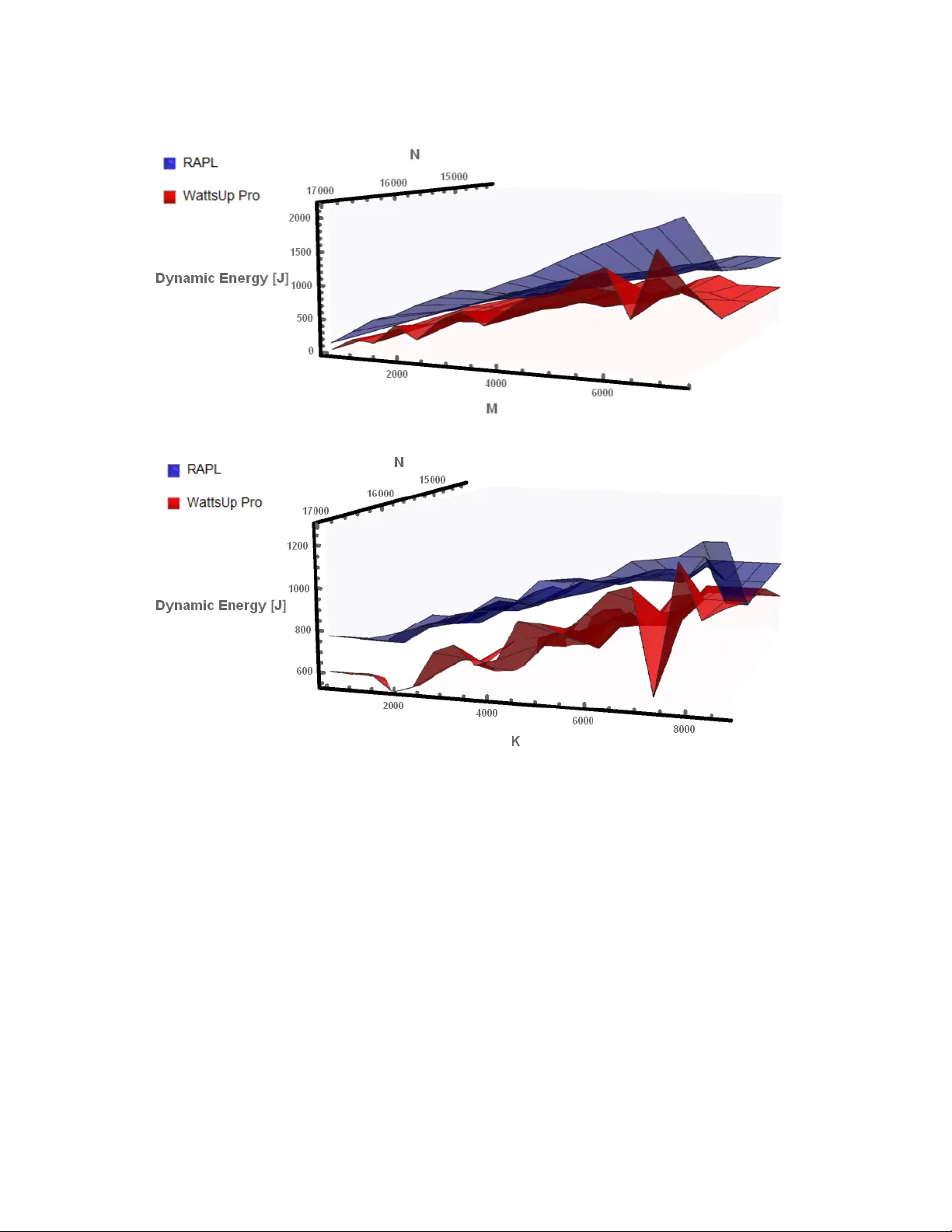
Original Paper
Loading high-quality paper...
Comments & Academic Discussion
Loading comments...
Leave a Comment