Online Optimization Methods for the Quantification Problem

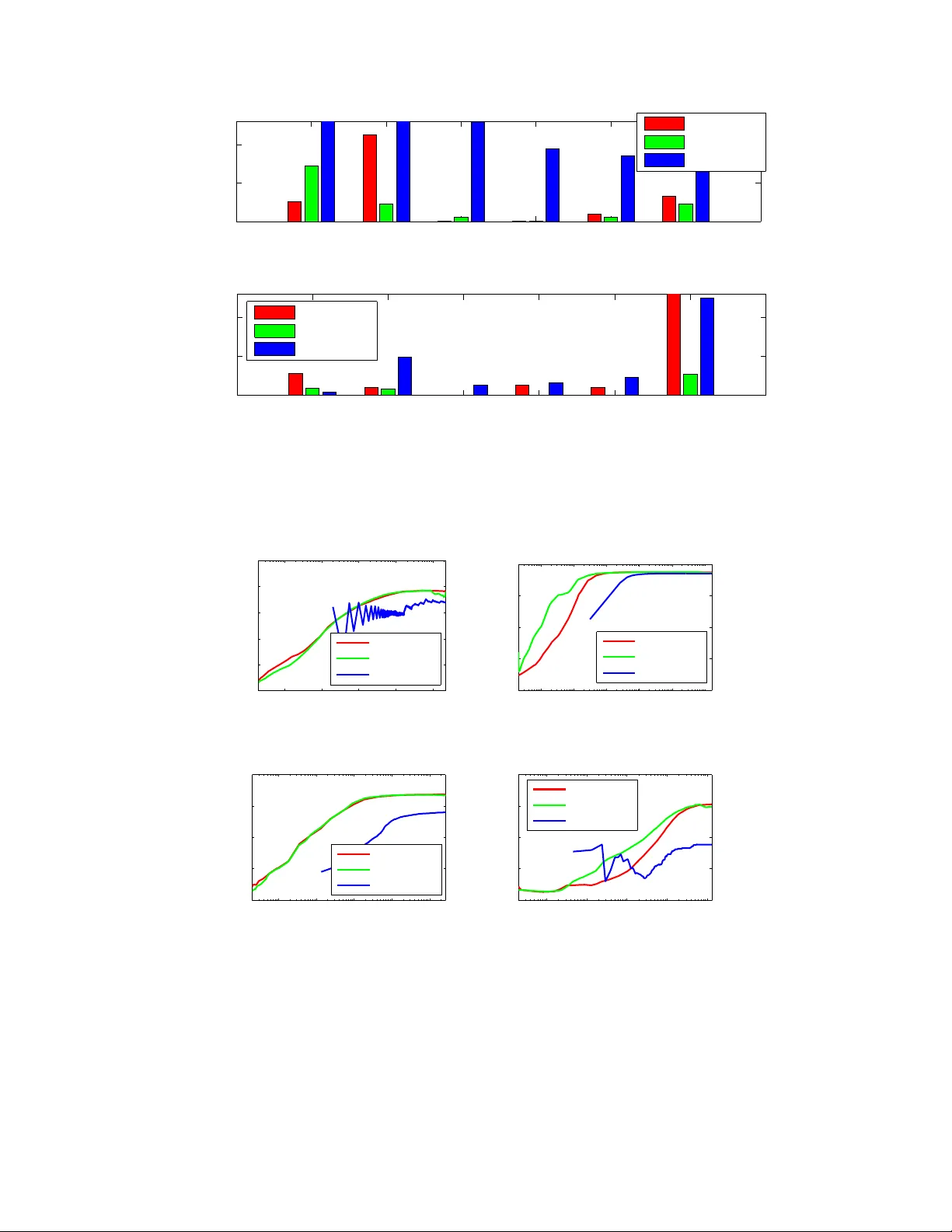
Online Optimization Methods for the Quantification Problem ∗ Purushottam Kar IIT Kanpur , India purushot@cse.iitk.ac.in Shuai Li † Uni versity of Insubria, Italy shuaili.sli@gmail.com Harikrishna Narasimhan Harv ard Univ ersity , USA hnarasimhan@g.harvard.edu Sanjay Chawla ‡ QCRI-HBKU, Qatar schawla@qf.org.qa Fabrizio Sebastiani § QCRI-HBKU, Qatar fsebastiani@qf.org.qa Abstract The estimation of class prev alence, i.e., the fraction of a population that belongs to a certain class, is a very useful tool in data analytics and learning, and finds applications in man y domains such as sentiment analysis, epidemiology , etc. For e xample, in sentiment analysis, the objecti ve is often not to estimate whether a specific text conv eys a positi ve or a negati ve sentiment, but rather estimate the o verall distrib ution of positiv e and negativ e sentiments during an event window . A popular way of performing the above task, often dubbed quantification , is to use supervised learning to train a prev alence estimator from labeled data. Contemporary literature cites se veral performance measures used to measure the success of such prev alence es- timators. In this paper we propose the first online stochastic algorithms for dir ectly optimizing these quantification- specific performance measures. W e also provide algorithms that optimize hybrid performance measures that seek to balance quantification and classification performance. Our algorithms present a significant advancement in the theory of multiv ariate optimization and we show , by a rigorous theoretical analysis, that they exhibit optimal con ver - gence. W e also report extensi ve experiments on benchmark and real data sets which demonstrate that our methods significantly outperform existing optimization techniques used for these performance measures. 1 Intr oduction Quantification [11] is defined as the task of estimating the prev alence (i.e., relati ve frequency) of the classes of interest in an unlabeled set, giv en a training set of items labeled according to the same classes. Quantification finds its natural application in contexts characterized by distribution drift , i.e., conte xts where the training data may not exhibit the same class pre valence pattern as the test data. This phenomenon may be due to dif ferent reasons, including the inherent non-stationary character of the context, or class bias that af fects the selection of the training data. ∗ A short v ersion of this manuscript will appear in the proceedings of the 22nd ACM SIGKDD Conference on Knowledge Discovery and Data Mining, KDD 2016. † This work was done while Shuai Li was a research associate at QCRI-HBKU. ‡ Sanjay Chawla is on lea ve from University of Sydne y . § Fabrizio Sebastiani is on lea ve from Consiglio Nazionale delle Ricerche, Italy . 1 A na ¨ ıve way to tackle quantification is via the “classify and count” (CC) approach, i.e., to classify each unlabeled item independently and compute the fraction of the unlabeled items that have been attributed to each class. Ho we ver , a good classifier does not necessarily lead to a good quantifier: assuming the binary case, ev en if the sum (FP + FN) of the false positi ves and f alse negati ves is comparativ ely small, bad quantification accuracy might result if FP and FN are significantly dif ferent (since perfect quantification coincides with the case FP = FN). This has led researchers to study quantification as a task in its own right, rather than as a byproduct of classification. The fact that quantification is not just classification in disguise can also be seen by the fact that e valuation mea- sures different from those for classification (e.g., F 1 , A UC) need to be employed. Quantification actually amounts to computing ho w well an estimated class distribution ˆ p fits an actual class distribution p (where for any class c ∈ C , p ( c ) and ˆ p ( c ) respecti vely denote its true and estimated prev alence); as such, the natural way to ev aluate the quality of this fit is via a function from the class of f -diver gences [7], and a natural choice from this class (if only for the fact that it is the best known f -diver gence) is the K ullback-Leibler Diver gence (KLD), defined as KLD ( p, ˆ p ) = X c ∈C p ( c ) log p ( c ) ˆ p ( c ) (1) Indeed, KLD is the most frequently used measure for ev aluating quantification (see e.g., [3, 10, 11, 12]). Note that KLD is non-decomposable, i.e., the error we make by estimating p via ˆ p cannot be broken do wn into item-le vel errors. This is not just a feature of KLD, but an inherent feature of any measure for e valuating quantification. In fact, how the error made on a giv en unlabeled item impacts the overall quantification error depends on how the other items have been classified 1 ; e.g., if FP > FN for the other unlabeled items, then generating an additional false ne gative is actually beneficial to the ov erall quantification accuracy , be it measured via KLD or via any other function. The fact that KLD is the measure of choice for quantification and that it is non-decomposable, has lead to the use of structured output learners, such as SVM perf [17], that allow a direct optimization of non-decomposable functions; the approach of Esuli and Sebastiani [9, 10] is indeed based on optimizing KLD using SVM perf . Ho wever , that minimizing KLD (or | FP − FN | , or any “pure” quantification measure) should be the only objecti ve for quantification regardless of the value of FP + FN (or any other classification measure), is fairly paradoxical. Some authors [3, 24] have observed that this might lead to the generation of unreliable quantifiers (i.e., systems with good quantification accuracy but bad or very bad classification accuracy), and hav e, as a result, championed the idea of optimizing “multi-objectiv e” measures that combine quantification accuracy with classification accuracy . Using a decision-tree-like approach, [24] minimizes | FP 2 − FN 2 | , which is the product of | FN − FP | , a measure of quantification error , and ( FN + FP ) , a measure of classification error; [3] also optimizes (using SVM perf ) a measure that combines quantification and classification accuracy . While SVM perf does provide a recipe for optimizing general performance measures, it has serious limitations. SVM perf is not designed to directly handle applications where large streaming data sets are the norm. SVM perf also does not scale well to multi-class settings, and the time required by the method is e xponential in the number of classes. In this paper we develop stochastic methods for optimizing a large family of popular quantification performance measures. Our methods can effortlessly work with streaming data and scale to very large datasets, offering training times up to an order of magnitude faster than other approaches such as SVM perf . 2 Related W ork Quantification methods. The quantification methods that have been proposed over the years can be broadly classified into two classes, namely aggre gativ e and non-aggregati ve methods. While a ggr egative approaches perform quantifica- tion by first classifying individual items as an intermediate step, non-aggr e gative approaches do not require this step, and estimate class prev alences holistically . Most methods, such as those of [3, 4, 10, 11, 24], fall in the former class, while the latter class has few representati ves [14, 22]. 1 For the sake of simplicity , we assume here that quantification is to be tackled in an aggr egative way , i.e., the classification of individual items is a necessary intermediate step for the estimation of class prev alences. Note howe ver that this is not necessary; non-aggregativ e approaches to quantification may be found in [14, 22]. 2 W ithin the class of aggregati ve methods, a further distinction can be made between methods, such as those of [4, 11], that first use general-purpose learning algorithms and then post-process their prev alence estimates to account for their estimation biases, and methods (which we ha ve already hinted at in Section 1) that instead use learning algo- rithms explicitly de vised for quantification [3, 10, 24]. In this paper we focus the latter class of methods. Applications of quantification. From an application perspective, quantification is especially useful in fields (such as social science, political science, market research, and epidemiology) which are inherently interested in aggregate data, and care little about individual cases. Aside from applications in these fields [16, 22], quantification has also been used in contexts as di verse as natural language processing [6], resource allocation [11], tweet sentiment analysis [12], and the veterinary sciences [14]. Quantification has independently been studied within statistics [16, 22], machine learning [2, 8, 29], and data mining [10, 11]. Unsurprisingly , gi ven this v aried literature, quantification also goes under different names, such as counting [23], class probability r e-estimation [1], class prior estimation [6], and learning of class balance [8]. In some applications of quantification, the estimation of class prev alences is not an end in itself, b ut is rather used to improv e the accuracy of other tasks such as classification. For instance, Balikas et al. [2] use quantification for model selection in supervised learning, by tuning hyperparameters that yield the best quantification accuracy on v alidation data; this allows hyperparameter tuning to be performed without incurring the costs inherent to k -fold cross-validation. Saerens et al. [29], followed by other authors [1, 32, 34], apply quantification to customize a trained classifier to the class pre valence e xhibited in the test set, with the goal of impro ving classification accuracy on unlabeled data e xhibit- ing a class distribution different from that of the training set. The work of Chan and Ng [6] may be seen as a direct application of this notion, as they use quantification to tune a word sense disambiguator to the estimated sense priors of the test set. Their work can also be seen as an instance of transfer learning (see e.g., [26]), since their goal is to adapt a word sense disambiguation algorithm to a domain dif ferent from the one the algorithm was trained upon. Stochastic optimization. As discussed in Section 1, our goal in this paper is to perform quantification by directly optimizing, in an online stochastic setting, specific performance measures for the quantification problem. While recent advances have seen much progress in efficient methods for online learning and optimization in full information and bandit settings [5, 13, 15, 30], these works frequently assume that the optimization objecti ve, or the notion of regret being considered is decomposable and can be written as a sum or expectation of losses or penalties on indi vidual data points. Howe ver , performance measures for quantification ha ve a multi variate and comple x structure, and do not hav e this form. There has been some recent progress [20, 25] tow ards dev eloping stochastic optimization methods for such non- decomposable measures. Howe ver , these approaches do not satisfy the needs of our problem. The work of Kar et al. [20] addresses the problem of optimizing structured SVM perf -style objectives in a streaming fashion, but requires the maintenance of large buf fers and, as a result, offers poor con ver gence. The work of Narasimhan et al. [25] presents online stochastic methods for optimizing performance measures that are concav e or pseudo-linear in the canonical confusion matrix of the predictor . Howe ver , their method requires the computation of gradients of the Fenchel dual of the performance measures, which is difficult for the quantification performance measures that we study , that have a nested structure. Our methods extend the work of [25] and provide con venient routines for optimizing the more complex performance measures used for e valuating quantification. 3 Pr oblem Setting For the sak e of simplicity , in this paper we will restrict our analysis to binary classification problems and linear models. W e will denote the space of feature v ectors by X ⊂ R d and the label set by Y = {− 1 , +1 } . W e shall assume that data points are generated according to some fixed but unknown distribution D over X × Y . W e will denote the proportion of positiv es in the population by p := Pr ( x ,y ) ∼D [ y = +1] . Our algorithms, at training time, will receiv e a set of T training points sampled from D , which we will denote by T = { ( x 1 , y 1 ) , . . . , ( x T , y T ) } . 3 As mentioned abov e, we will present our algorithms and analyses for learning a linear model over X . W e will de- note the model space by W ⊆ R d and let R X and R W denote the radii of domain X and model space W , respecti vely . Howe ver , we note that our algorithms and analyses can be e xtended to learning non-linear models by use of kernels, as well as to multi-class quantification problems. Howe ver , we postpone a discussion of these extensions to an e xpanded version of this paper . Our focus in this work shall be the optimization of quantification-specific performance measures in online stochas- tic settings. W e will concentrate on performance measures that can be represented as functions of the confusion matrix of the classifier . In the binary setting, the confusion matrix can be completely described in terms of the true positive rate (TPR) and the true negati ve rate (TNR) of the classifier . Howe ver , initially we will de velop algorithms that use r ewar d functions as surrogates of the TPR and TNR values. This is done to ease algorithm design and analysis, since the TPR and TNR v alues are count-based and form non-concav e and non-dif ferentiable estimators. The surrogates we will use will be conca ve and almost-ev erywhere differentiable. More formally , we will use a rew ard function r that assigns a r ewar d r ( ˆ y , y ) to a prediction ˆ y ∈ R for a data point, when the true label for that data point is y ∈ Y . Giv en a rew ard function r , a model w ∈ W , and a data point ( x , y ) ∈ X × Y , we will use r + ( w ; x , y ) = 1 p · r ( w > x , y ) · 1 ( y = 1) r − ( w ; x , y ) = 1 1 − p · r ( w > x , y ) · 1 ( y = − 1) to calculate re wards on positi ve and ne gative points. The a verage or expected value of these rew ards will be treated as surrogates of TPR and TNR respecti vely . Note that since E ( x ,y ) J r + ( w ; x , y ) K = E ( x ,y ) q r ( w > x , y ) | y = 1 y , set- ting r to r 0 - 1 ( ˆ y , y ) = I [ y · ˆ y > 0] , i.e. the classification accuracy function, yields E ( x ,y ) J r + ( w ; x , y ) K = TPR ( w ) . Here I [ · ] denotes the indicator function. For the sake of con venience we will use P ( w ) = E ( x ,y ) J r + ( w ; x , y ) K and N ( w ) = E ( x ,y ) J r − ( w ; x , y ) K to denote population averages of the reward functions. W e shall assume that our reward function r is concav e, L r -Lipschitz, and takes v alues in a bounded range [ − B r , B r ] . Examples of Surr ogate Reward Functions Some examples of re ward functions that are surrogates for the classifica- tion accuracy indicator function I [ y ˆ y > 0] are the inv erted hinge loss function r hinge ( ˆ y , y ) = max { 1 , y · ˆ y } and the in verted logistic regression function r logit ( ˆ y , y ) = 1 − ln(1 + exp( − y · ˆ y )) W e will also experiment with non-surrogate (dubbed NS) versions of our algorithms which use TPR and TNR values directly . These will be discussed in Section 5. 3.1 Perf ormance Measur es The task of quantification requires estimating the distribution of unlabeled items across a set C of av ailable classes, with |C | = 2 in the binary setting. In our w ork we will tar get quantification performance measures as well as “hybrid” classification-quantification performance measures. W e discuss them in turn. KLD: Kullback-Leibler Div ergence In recent years this performance measure has become a standard in the quan- tification literature, in the ev aluation of both binary and multiclass quantification [3, 10, 12]. W e redefine KLD below for con venience. KLD ( p, ˆ p ) = X c ∈C p ( c ) log p ( c ) ˆ p ( c ) (2) 4 For distributions p, p 0 ov er C , the values KLD ( p, p 0 ) can range between 0 (perfect quantification) and + ∞ . 2 . Note that since KLD is a distance function and all our algorithms will be driv en by rew ard maximization, for uniformity we will, instead of trying to minimize KLD, try to maximize − KLD; we will call this latter NegKLD. NSS: Normalized Squared Score This measure of quantification accuracy was introduced in [3], and is defined as NSS = 1 − ( FN − FP max { p, (1 − p ) }|S | ) 2 . Ignoring normalization constants, this performance measure attempts to reduce | FN − FP | , a direct measure of quantification error . W e recall from Section 1 that several works ha ve advocated the use of hybrid, “multi-objecti ve” performance mea- sures, that try to balance quantification and classification performance. These measures typically take a quantification performance measure such as KLD or NSS, and combine it with a classification performance measure. T ypically , a classification performance measure that is sensitiv e to class imbalance [25] is chosen, such as Balanced Accuracy B A = 1 2 ( TPR + TNR ) [3], F-measure, or G-mean [25]. T wo such hybrid performance measures that are discussed in literature are presented below . CQB: Classification-Quantification Balancing The work of [24] introduced this performance measure in an attempt to compromise between classification and quantification accuracy . As discussed in Section 1, this performance mea- sure is defined as CQB = | FP 2 − FN 2 | = | FP − FN | · ( FP + FN ) , i.e. a product of | FN − FP | , a measure of quantification error , and ( FN + FP ) , a measure of classification error . QMeasure The work of Barranquero et al. [3] introduced a generic scheme for constructing hybrid performance measures, using the so-called Q-measure defined as Q β = (1 + β 2 ) · P class · P quant β 2 P class + P quant , (3) that is, a weighted combination of a measure of classification accuracy P class and a measure of quantification accuracy P quant . For the sake of simplicity , in our experiments we will adopt B A = 1 2 ( TPR + TNR ) as our P class and NSS as our P quant . Howe ver , we stress that our methods can be suitably adapted to work with other choices of P class and P quant . W e also introduce three ne w hybrid performance measures in this paper as a w ay of testing our optimization algo- rithms. W e define these below and refer the reader to T ables 1 and 2 for details. B AKLD This hybrid performance measure takes a weighted average of BA and NegKLD; i.e. BAKLD = C · BA + (1 − C ) · ( − KLD ) . This performance measure gives the user a strong handle on how much emphasis should be placed on quantification and how much on classification performance. W e will use BAKLD in our experiments to show that our methods offer an attracti ve tradeof f between the two. 2 KLD is not a particularly well-beha ved performance measure, since it is capable of taking unbounded v alues within the compact domain of the unit simplex. This poses a problem for optimization algorithms from the point of view of con vergence, as well as numerical stability . T o solve this problem, while computing KLD for two distributions p and ˆ p , we can perform an additive smoothing of both p ( c ) and ˆ p ( c ) by computing p s ( c ) =  + p ( c )  |C | + X c ∈C p ( c ) where p s ( c ) denotes the smoothed version of p ( c ) . The denominator here is just a normalizing factor . The quantity  = 1 2 |S | is often used as a smoothing factor , and is the one we adopt here. The smoothed versions of p ( c ) and ˆ p ( c ) are then used in place of the non-smoothed versions in Equation 1. W e can show that, as a result, KLD is always bounded by KLD ( p s , ˆ p s ) ≤ O  log 1   Howe ver , we note that the smoothed KLD still returns a value of 0 when p and ˆ p are identical distributions. 5 W e now define two hybrid performance measures that are constructed by taking the ratio of a classification and a quantification performance measures. The aim of this ex ercise is to obtain performance measures that mimic the F-measure, which is also a pseudolinear performance measure [25]. The ability of our methods to directly optimize such complex performance measures will be indicativ e of their utility in terms of the freedom they allow the user to design objectiv es in a data- and task-specific manner . CQReward and BKReward These hybrid performance measures are defined as CQReward = BA 2 − NSS and BKReward = BA 1+ KLD . Notice that both performance measures are optimized when the numerator i.e. B A is large, and the denomi- nator is small which translates to NSS being large for CQReward and KLD being small for BKReward. Clearly , both performance measures encourage good performance with respect to both classification and quantification and penalize a predictor which either neglects quantification to get better classification performance, or the other way round. The past section has seen us introduce a wide variety of quantification and hybrid performance measures. Of these, the NegKLD, NSS, and Q-measure were already prev alent in quantification literature and we introduced BAKLD, CQRew ard and BKRew ard. As discussed before, the aim of exploring such a large variety of performance measures is to both demonstrate the utility of our methods with respect to the quantification problem, and present newer ways of designing hybrid performance measures that give the user more expressi vity in tailoring the performance measure to the task at hand. W e also note that these performance measures have extremely diverse and complex structures. W e can show that NegKLD, Q-measure, and B AKLD are nested concav e functions, more specifically , concave functions of functions that are themselves concave in the confusion matrix of the predictor . On the other hand, CQReward and BKRew ard turn out to be pseudo-conca ve functions of the confusion matrix. Thus, we are working with tw o very different families of performance measures here, each of which has different properties and requires dif ferent optimization techniques. In the following section, we introduce tw o novel methods to optimize these tw o families of performance measures. 4 Stochastic Optimization Methods f or Quantification The previous discussion in Sections 1 and 2 clarifies two aspects of efforts in the quantification literature. Firstly , specific performance measures hav e been developed and adopted for ev aluating quantification performance including KLD, NSS, Q-measure etc. Secondly , algorithms that directly optimize these performance measures are desirable, as is evidenced by recent w orks [3, 9, 10, 24]. The works mentioned abo ve make use of tools from optimization literature to learn linear (e.g. [10]) and non-linear (e.g. [24]) models to perform quantification. The state of the art ef forts in this direction ha ve adopted the structural SVM approach for optimizing these performance measures with great success [3, 10]. Howe ver , this approach comes with sev ere drawbacks. The structural SVM [17], although a significant tool that allows optimization of arbitrary performance measures, suffers from two key drawbacks. Firstly , the structural SVM surrogate is not necessarily a tight surrogate for all performance measures, something that has been demonstrated in past literature [21, 25], which can lead to poor training. But more importantly , optimizing the structural SVM surrogate requires the use of expensi ve cutting plane methods which are known to scale poorly with the amount of training data, as well as are unable to handle streaming data. T o alle viate these problems, we propose stochastic optimization algorithms that dir ectly optimize a lar ge family of quantification performance measures. Our methods come with sound theoretical conv ergence guarantees, are able to operate with streaming data sets and, as our experiments will demonstrate, offer much faster and accurate quantification performance on a variety of data sets. Our optimization techniques introduce crucial advancements in the field of stochastic optimization of multivariate performance measur es and address the two families of performance measures discussed while concluding Section 3 – 1) nested conca ve performance measures and 2) pseudo-concave performance measures. W e describe these in turn below . 6 T able 1: A list of nested conca ve performance measures and their canonical e xpressions in terms of the confusion ma- trix Ψ( P , N ) where P and N denote the TPR, TNR v alues and p and n denote the proportion of positi ves and negati ves in the population. The 4th, 6th and 8th columns giv e the closed form updates used in steps 15-17 in Algorithm 1. Name Expression Ψ( x, y ) γ ( q ) ζ 1 ( P , N ) α ( r ) ζ 2 ( P , N ) β ( r ) NegKLD [3, 10] − KLD ( p, ˆ p ) p · x + n · y ( p,n ) log ( pP + n (1 − N ))  1 r 1 , 1 r 2  log( nN + p (1 − P ))  1 r 1 , 1 r 2  QMeasure β [3] (1+ β 2 ) · BA · NSS β 2 · BA + NSS (1+ β 2 ) · x · y β 2 · x + y (1+ β 2 ) ·  z 2 , (1 − z ) 2 β 2  z = q 2 β 2 q 1 + q 2 P + N 2 ( 1 2 , 1 2 ) 1 − ( p (1 − P ) − n (1 − N )) 2 2( z, − z ) z = r 2 − r 1 B AKLD C · BA +(1 − C ) · ( − KLD ) C · x +(1 − C ) · y ( C, 1 − C ) P + N 2 ( 1 2 , 1 2 ) − KLD ( P,N ) see abov e 4.1 Nested Conca ve Perf ormance Measures The first class of performance measures that we deal with are conca ve combinations of conca ve performance measures. More formally , given three conca ve functions Ψ , ζ 1 , ζ 2 : R 2 → R , we can define a performance measure P (Ψ ,ζ 1 ,ζ 2 ) ( w ) = Ψ( ζ 1 ( w ) , ζ 2 ( w )) , where we hav e ζ 1 ( w ) = ζ 1 ( P ( w ) , N ( w )) ζ 2 ( w ) = ζ 2 ( P ( w ) , N ( w )) , where P ( w ) and N ( w ) can respectiv ely denote, either the TPR and TNR values or surrogate re ward functions therefor . Examples of such performance measures include the negati ve KLD performance measure and the QMeasure which are described in Section 3.1. T able 1 describes these performance measures in canonical form i.e. their expressions in terms of TPR and TNR values. Before describing our algorithm for nested conca ve measures, we recall the notion of concav e Fenchel conjugate of concav e functions. For any conca ve function f : R 2 → R and any ( u, v ) ∈ R 2 , the (concav e) Fenchel conjugate of f is defined as f ∗ ( u, v ) = inf ( x,y ) ∈ R 2 { ux + v y − f ( x, y ) } . Clearly , f ∗ is concav e. Moreover , it follo ws from the concavity of f that for any ( x, y ) ∈ R 2 , f ( x, y ) = inf ( u,v ) ∈ R 2 { xu + y v − f ∗ ( u, v ) } . Below we state the properties of strong concavity and smoothness. These will be crucial in our con vergence analysis. Definition 1 (Strong Concavity and Smoothness) . A function f : R d → R is said to be α -str ongly concave and γ -smooth if for all x , y ∈ R d , we have − γ 2 k x − y k 2 2 ≤ f ( x ) − f ( y ) − h∇ f ( y ) , x − y i ≤ − α 2 k x − y k 2 2 . W e will assume that the functions Ψ , ζ 1 , and ζ 2 defining our performance measures are γ -smooth for some constant γ > 0 . This is true of all functions, save the log function which is used in the definition of the KLD quantification measure. Ho wever , if we carry out the smoothing step pointed out in Section 3.1 with some  > 0 , then it can be shown that the KLD function does become O  1  2  -smooth. An important property of smooth functions, that would be crucial in our analyses, is a close relationship between smooth and strongly con vex functions Theorem 2 ([33]) . A closed, concave function f is β smooth iff its (concave) F enchel conjugate f ∗ is 1 β -str ongly concave. 7 Algorithm 1 NEMSIS : NEsted priMal-dual StochastIc updateS Require: Outer wrapper function Ψ , inner performance measures ζ 1 , ζ 2 , step sizes η t , feasible sets W , A Ensure: Classifier w ∈ W 1: w 0 ← 0 , t ← 0 , { r 0 , q 0 , α 0 , β 0 , γ 0 } ← (0 , 0) 2: while data stream has points do 3: Receiv e data point ( x t , y t ) 4: // Perform primal ascent 5: if y t > 0 then 6: w t +1 ← Π W  w t + η t ( γ t, 1 α t, 1 + γ t, 2 β t, 1 ) ∇ w r + ( w t ; x t , y t )  7: q t +1 ← t · q t + ( α t, 1 , β t, 1 ) · r + ( w t ; x t , y t ) 8: else 9: w t +1 ← Π W  w t + η t ( γ t, 1 α t, 2 + γ t, 2 β t, 2 ) ∇ w r − ( w t ; x t , y t )  10: q t +1 ← t · q t + ( α t, 2 , β t, 2 ) · r − ( w t ; x t , y t ) 11: end if 12: r t +1 ← ( t + 1) − 1  t · r t + ( r + ( w t ; x t , y t ) , r − ( w t ; x t , y t ))  13: q t +1 ← ( t + 1) − 1 ( q t +1 − ( ζ ∗ 1 ( α t ) , ζ ∗ 2 ( β t ))) 14: // Perform dual updates 15: α t +1 = arg min α { α · r t +1 − ζ ∗ 1 ( α ) } 16: β t +1 = arg min β { β · r t +1 − ζ ∗ 2 ( β ) } 17: γ t +1 = arg min γ { γ · q t +1 − Ψ ∗ ( γ ) } 18: t ← t + 1 19: end while 20: r eturn w = 1 t P t τ =1 w τ W e are no w in a position to present our algorithm NEMSIS for stochastic optimization of nested concav e functions. Algorithm 1 gives an outline of the technique. W e note that a direct application of traditional stochastic optimization techniques [31] to such nested performance measures as those considered here is not possible as discussed before. NEMSIS , overcomes these challenges by e xploiting the nested dual structure of the performance measure by carefully balancing updates at the inner and outer lev els. At ev ery time step, NEMSIS performs four very cheap updates. The first update is a primal ascent update to the model vector which takes a weighted stochastic gradient descent step. Note that this step inv olves a pr ojection step to the set of model vectors W denoted by Π W ( · ) . In our experiments W was defined to be the set of all Euclidean norm-bounded vectors so that projection could be ef fected using Euclidean normalization which can be done in O ( d ) time if the model vectors are d -dimensional. The weights of the descent step are decided by the dual parameters of the functions Ψ , ζ 1 , and ζ 2 . Then NEMSIS updates the dual variables in three simple steps. In fact line numbers 15-17 can be executed in closed form (see T able 1) for all the performance measures we see here which allo ws for very rapid updates. See Appendix A for the simple deriv ations. Below we state the conv ergence proof for NEMSIS . W e note that despite the complicated nature of the perfor- mance measures being tackled, NEMSIS is still able to recover the optimal rate of con vergence kno wn for stochastic optimization routines. W e refer the reader to Appendix B for a proof of this theorem. The proof requires a careful analysis of the primal and dual update steps at different le vels and tying the updates together by taking into account the nesting structure of the performance measure. Theorem 3. Suppose we ar e given a stream of random samples ( x 1 , y 1 ) , . . . , ( x T , y T ) drawn fr om a distribution D over X × Y . Let Algorithm 1 be executed with step sizes η t = Θ(1 / √ t ) with a nested concave performance measur e Ψ( ζ 1 ( · ) , ζ 2 ( · )) . Then, for some universal constant C , the averag e model w = 1 T P T t =1 w t output by the algorithm satisfies, with pr obability at least 1 − δ , P (Ψ ,ζ 1 ,ζ 2 ) ( w ) ≥ sup w ∗ ∈W P (Ψ ,ζ 1 ,ζ 2 ) ( w ∗ ) − C Ψ ,ζ 1 ,ζ 2 ,r ·  log 1 δ √ T  , 8 T able 2: List of pseudo-concave performance measures and their canonical expressions in terms of the confusion matrix Ψ( P , N ) . Note that p and n denote the proportion of positiv es and negativ es in the population. Name Expression P quant ( P , N ) P class ( P , N ) CQRew ard BA 2 − NSS 1+( p (1 − P ) − n (1 − N )) 2 P + N 2 BKRew ard BA 1+ KLD KLD: see T able 1 P + N 2 wher e C Ψ ,ζ 1 ,ζ 2 ,r = C ( L Ψ ( L r + B r )( L ζ 1 + L ζ 2 )) for a universal constant C and L g denotes the Lipsc hitz constant of the function g . Related work of Narasimhan et al : Narasimhan et al [25] proposed an algorithm SP ADE which of fered stochastic optimization of conca ve performance measures. W e note that although the performance measures considered here are indeed concave, it is difficult to apply SP ADE to them directly since SP ADE requires computation of gradients of the Fenchel dual of the function P (Ψ ,ζ 1 ,ζ 2 ) which are difficult to compute giv en the nested structure of this function. NEMSIS , on the other hand, only requires the duals of the indi vidual functions Ψ , ζ 1 , and ζ 2 which are much more accessible. Moreover , NEMSIS uses a much simpler dual update which does not inv olve any parameters and, in fact, has a closed form solution in all our cases. SP ADE , on the other hand, performs dual gradient descent which requires a fine tuning of yet another step length parameter . A third benefit of NEMSIS is that it achieves a logarithmic regret with respect to its dual updates (see the proof of Theorem 3) whereas SP ADE incurs a polynomial regret due to its gradient descent-style dual update. 4.2 Pseudo-conca ve Perf ormance Measures The next class of performance measures we consider can be expressed as a ratio of a quantification and a classifica- tion performance measure. More formally , giv en a con vex quantification performance measure P quant and a concave classification performance measure P class , we can define a performance measure P ( P quant , P class ) ( w ) = P class ( w ) P quant ( w ) , W e assume that both the performance measures, P quant and P class , are positi ve valued. Such performance measures can be very useful in allowing a system designer to balance classification and quantification performance. Moreov er, the form of the measure allows an enormous amount of freedom in choosing the quantification and classification performance measures. Examples of such performance measures include the CQRe ward and the BKRew ard measures. These were introduced in Section 3.1 and are represented in their canonical forms in T able 2. Performance measures, constructed the way described above, with a ratio of a concav e over a conv ex measures, are called pseudo-concave measures. This is because, although these functions are not concav e, their lev el sets are still con vex which makes it possible to optimize them ef ficiently . T o see the intuition behind this, we need to introduce the notion of the valuation function corresponding to the performance measure. As a passing note, we remark that because of the non-concavity of these performance measures, NEMSIS cannot be applied here. Definition 4 (V aluation Function) . The valuation of a pseudo-concave performance measure P ( P quant , P class ) ( w ) = P class ( w ) P quant ( w ) at any level v > 0 , is defined as V ( w , v ) = P class ( w ) − v · P quant ( w ) It can be seen that the valuation function defines the le vel sets of the performance measure. T o see this, notice that due to the positivity of the functions P quant and P class , we can have P ( P quant , P class ) ( w ) ≥ v iff V ( w , v ) ≥ 0 . Howe ver , since P class is concav e, P quant is con vex, and v > 0 , V ( w , v ) is a conca ve function of w . This close connection between the le vel sets and notions of v aluation functions ha ve been exploited before to gi ve optimization algorithms for pseudo-linear performance measures such as the F-measure [25, 27]. These approaches treat the valuation function as some form of proxy or surrogate for the original performance measure and optimize it in hopes of making progress with respect to the original measure. 9 Algorithm 2 CAN : Concav e AlternatioN Require: Objective P ( P quant , P class ) , model space W , tolerance  Ensure: An  -optimal classifier w ∈ W 1: Construct the v aluation function V 2: w 0 ← 0 , t ← 1 3: while v t > v t − 1 +  do 4: w t +1 ← arg max w ∈W V ( w , v t ) 5: v t +1 ← arg max v> 0 v such that V ( w t +1 , v ) ≥ v 6: t ← t + 1 7: end while 8: r eturn w t T aking this approach with our performance measures yields a very natural algorithm for optimizing pseudo- concav e measures which we outline in the CAN algorithm Algorithm 2. CAN repeatedly trains models to optimize their v aluations at the current level, then upgrades the level itself. Notice that step 4 in the algorithm is a concave maximization problem over a conv ex set, something that can be done using a v ariety of methods – in the following we will see how NEMSIS can be used to implement this step. Also notice that step 5 can, by the definition of the valuation function, be carried out by simply setting v t +1 = P ( P quant , P class ) ( w t +1 ) . It turns out that CAN has a linear rate of con vergence for well-behav ed performance measures. The next result formalizes this statement. W e note that this result is similar to the one arriv ed by [25] but only for pseudo-linear functions. Theorem 5. Suppose we execute Algorithm 2 with a pseudo-concave performance measur e P ( P quant , P class ) such that the quantification performance measur e always takes values in the range [ m, M ] , wher e M > m > 0 . Let P ∗ := sup w ∈W P ( P quant , P class ) ( w ) be the optimal performance level and ∆ t = P ∗ − P ( P quant , P class ) ( w t ) be the excess err or for the model w t generated at time t . Then, for every t > 0 , we have ∆ t ≤ ∆ 0 ·  1 − m M  t . W e refer the reader to Appendix C for a proof of this theorem. This theorem generalizes the result of [25] to the more general case of pseudo-concave functions. Note that for the pseudo-concave functions defined in T able 2, care is taken to ensure that the quantification performance measure satisfies m > 0 . A drawback of CAN is that it cannot operate in streaming data settings and requires a concave optimization oracle. Howe ver , we notice that for the performance measures in T able 2, the valuation function is always at least a nested concav e function. This motiv ates us to use NEMSIS to solve the inner optimization problems in an online fashion. Combining this with an online technique to approximately execute step 5 of of the CAN and giv es us the SCAN algorithm, outlined in Algorithm 3. Thoerem 6 shows that SCAN enjoys a conv ergence rate similar to that of NEMSIS . Indeed, SCAN is able to guarantee an  -approximate solution after witnessing e O  1 / 2  samples which is equi valent to a con vergence rate of e O  1 / √ T  . The proof of this result is obtained by showing that CAN is robust to approximate solutions to the inner optimization problems. W e refer the reader to Appendix D for a proof of this theorem. Theorem 6. Suppose we execute Algorithm 3 with a pseudo-concave performance measur e P ( P quant , P class ) such that P quant always takes values in the range [ m, M ] with m > 0 , with epoch lengths s e , s 0 e = C Ψ ,ζ 1 ,ζ 2 ,r m 2  M M − m  2 e following a geometric rate of incr ease, where the constant C Ψ ,ζ 1 ,ζ 2 ,r is the ef fective constant for the NEMSIS analysis (Theor em 3) for the inner in vocations of NEMSIS in SCAN . Also let the excess err or for the model w e generated after e epochs be denoted by ∆ e = P ∗ − P ( P quant , P class ) ( w e ) . Then after e = O  log  1  log 2 1   epochs, we can ensure with pr obability at least 1 − δ that ∆ e ≤  . Mor eover , the number of samples consumed till this point, ignoring universal constants, is at most C 2 Ψ ,ζ 1 ,ζ 2 ,r  2  log log 1  + log 1 δ  log 4 1  . 10 Algorithm 3 SCAN : Stochastic Concav e AlternatioN Require: Objective P ( P quant , P class ) , model space W , step sizes η t , epoch lengths s e , s 0 e Ensure: Classifier w ∈ W 1: v 0 ← 0 , t ← 0 , e ← 0 , w 0 ← 0 2: r epeat 3: // Learning phase 4: e w ← w e 5: while t < s e do 6: Receiv e sample ( x , y ) 7: // NEMSIS update with V ( · , v e ) at time t 8: w t +1 ← NEMSIS ( V ( · , v e ) , w t , ( x , y ) , t ) 9: t ← t + 1 10: end while 11: t ← 0 , e ← e + 1 , w e +1 ← e w 12: // Level estimation phase 13: v + ← 0 , v − ← 0 14: while t < s 0 e do 15: Receiv e sample ( x , y ) 16: v y ← v y + r y ( w e ; x , y ) // Collect rewards 17: t ← t + 1 18: end while 19: t ← 0 , v e ← P class ( v + ,v − ) P quant ( v + ,v − ) 20: until stream is e xhausted 21: r eturn w e T able 3: Statistics of data sets used. Data Set Data Points F eatures P ositives KDDCup08 102,294 117 0.61% PPI 240,249 85 1.19% Cov erT ype 581,012 54 1.63% ChemInfo 2142 55 2.33% Letter 20,000 16 3.92% IJCNN-1 141,691 22 9.57% Adult 48,842 123 23.93% Cod-RN A 488,565 8 33.3% Related work of Narasimhan et al : Narasimhan et al [25] also proposed tw o algorithms AMP and ST AMP which seek to optimize pseudo-linear performance measures. Howe ver , neither those algorithms nor their analyses transfer directly to the pseudo-concave setting. This is because, by exploiting the pseudo-linearity of the performance measure, AMP and ST AMP are able to conv ert their problem to a sequence of cost-weighted optimization problems which are very simple to solve. This con venience is absent here and as mentioned above, ev en after creation of the valuation function, SCAN still has to solve a possibly nested concave minimization problem which it does by in voking the NEMSIS procedure on this inner problem. The proof technique used in [25] for analyzing AMP also makes heavy use of pseudo-linearity . The con ver gence proof of CAN , on the other hand, is more general and yet guarantees a linear con vergence rate. 5 Experimental Results W e carried out an extensi ve set of experiments on div erse set of benchmark and real-world data to compare our pro- posed methods with other state-of-the-art approaches. 11 Data sets : W e used the follo wing benchmark data sets from the UCI machine learning repository : a) IJCNN, b) Cov ertype, c) Adult, d) Letters, and e) Cod-RNA. W e also used the following three real-world data sets: a) Chemin- formatics, a drug discovery data set from [19], b) 2008 KDD Cup challenge data set on breast cancer detection, and c) a data set pertaining to a protein-protein interaction (PPI) prediction task [28]. In each case, we used 70% of the data for training and the remaining for testing. Methods : W e compares our proposed NEMSIS and SCAN algorithms 3 against the state-of-the-art one-pass mini- batch stochastic gradient method ( 1PMB ) of [20] and the SVM perf technique of [18]. Both these techniques are capable of optimizing structural SVM surrogates of arbitrary performance measures and we modified their implementations to suitably adapt them to the performance measures considered here. The NEMSIS and SCAN implementations used the hinge-based concav e surrogate. Non-surrogate NS Appr oaches : W e also experimented with a v ariant of the NEMSIS and SCAN algorithms, where the dual updates were computed using original count based TPR and TNR values, rather than surrogate rew ard functions. W e refer to this version as NEMSIS-NS . W e also de veloped a similar version of SCAN called SCAN-NS where the le vel estimation was performed using 0-1 TPR/TNR values. W e empirically observed these non-surrogate versions of the algorithms to of fer superior and more stable performance than the surrogate versions. 10 −4 10 −3 10 −2 10 −1 10 0 −1 −0.8 −0.6 −0.4 −0.2 0 Training time (secs) Negative KLD NEMSIS NEMSIS−NS 1PMB SVMPerf (a) Adult 10 −4 10 −3 10 −2 10 −1 10 0 −2.5 −2 −1.5 −1 −0.5 0 Training time (secs) Negative KLD NEMSIS NEMSIS−NS 1PMB SVMPerf (b) Cod-RN A 10 −4 10 −3 10 −2 10 −1 10 0 −1 −0.8 −0.6 −0.4 −0.2 0 Training time (secs) Negative KLD NEMSIS NEMSIS−NS 1PMB SVMPerf (c) KDD08 10 −4 10 −3 10 −2 10 −1 10 0 −0.4 −0.3 −0.2 −0.1 0 Training time (secs) Negative KLD NEMSIS NEMSIS−NS 1PMB SVMPerf (d) PPI Figure 1: Experiments with NEMSIS on NegKLD: Plot of NegKLD as a function of training time. 3 W e will make code for our methods av ailable publicly . 12 0 0.2 0.4 0.6 0.8 1 −3 −0.1 −0.05 0 Negative KLD CWeight 0 0.2 0.4 0.6 0.8 1 −3 0 0.5 1 BA (a) Adult 0 0.2 0.4 0.6 0.8 1 −3 −0.03 −0.02 −0.01 0 Negative KLD CWeight 0 0.2 0.4 0.6 0.8 1 −3 0.4 0.6 0.8 1 BA (b) Cod-RN A 0 0.2 0.4 0.6 0.8 1 −3 −0.4 −0.2 0 Negative KLD CWeight 0 0.2 0.4 0.6 0.8 1 −3 0 0.5 1 BA (c) Covtype Figure 2: Experiments on NEMSIS with B AKLD: Plots of quantification and classification performance as CW eight is varied. 0 0.1 0.2 Positive KLD kdd08 0 0.5 1 1.5 Positive KLD ppi 0 0.5 1 Positive KLD covtype 0 0.02 0.04 0.06 Positive KLD chemo 0 1 2 3 x 10 −3 Positive KLD letter 0 0.1 0.2 Positive KLD ijcnn1 0 0.02 0.04 Positive KLD a9a 0 0.02 0.04 0.06 Positive KLD cod−rna Figure 3: A comparison of the KLD performance of various methods on data sets with varying class proportions (see T able 4.2). 13 40 60 80 100 120 140 0 0.05 0.1 % change in class proportion Positive KLD NEMSIS NEMSIS−NS 1PMB (a) Adult 40 60 80 100 120 140 0 0.05 0.1 % change in class proportion Positive KLD NEMSIS NEMSIS−NS 1PMB (b) Letter Figure 4: A comparison of the KLD performance of v arious methods when distribution drift is introduced in the test sets. 10 −4 10 −3 10 −2 10 −1 10 0 0.7 0.75 0.8 0.85 0.9 0.95 Training time (secs) QMeasure NEMSIS NEMSIS−NS 1PMB (a) Adult 10 −4 10 −3 10 −2 10 −1 10 0 0.7 0.8 0.9 1 Training time (secs) QMeasure NEMSIS NEMSIS−NS 1PMB (b) Cod-RN A 10 −4 10 −3 10 −2 10 −1 10 0 0.7 0.8 0.9 1 Training time (secs) QMeasure NEMSIS NEMSIS−NS 1PMB (c) IJCNN1 10 −4 10 −3 10 −2 10 −1 10 0 0.7 0.8 0.9 1 Training time (secs) QMeasure NEMSIS NEMSIS−NS 1PMB (d) KDD08 Figure 5: Experiments with NEMSIS on Q-measure: Plot of Q-measure performance as a function of time. 14 10 −4 10 −3 10 −2 10 −1 10 0 0.7 0.8 0.9 1 Training time (secs) CQReward SCAN−NS 1PMB (a) Adult 10 −4 10 −3 10 −2 10 −1 10 0 0.7 0.8 0.9 1 Training time (secs) CQReward SCAN−NS 1PMB (b) Cod-RN A 10 −4 10 −3 10 −2 10 −1 10 0 0.4 0.5 0.6 0.7 0.8 0.9 Training time (secs) CQReward SCAN−NS 1PMB (c) CovT ype 10 −4 10 −3 10 −2 10 −1 10 0 0.5 0.6 0.7 0.8 0.9 1 Training time (secs) CQReward SCAN−NS 1PMB (d) IJCNN1 Figure 6: Experiments with SCAN on CQrew ard: Plot of CQreward performance as a function of time. Parameters : All parameters including step sizes, upper bounds on rew ard functions, regularization parameters, and projection radii were tuned from the values { 10 − 4 , 10 − 3 , . . . , 10 3 , 10 4 } using a held-out portion of the training set treated as a v alidation set. For step sizes, the base step length η 0 was tuned from the abo ve set and the step lengths were set to η t = η 0 / √ t . In 1PMB , we mimic the parameter setting in [20], setting the buf fer size to 500 and the number of passes to 25. Comparison on NegKLD: W e first compare NEMSIS-NS and NEMSIS against the baselines 1PMB and SVM perf on several data sets on the negativ e KLD measure. The results are presented in Figure 1. It is clear that the proposed algorithms have comparable performance with significantly faster rate of conv ergence. Since SVM perf is a batch/off- line method, it is important to clarify how it was compared against the other online methods. In this case, timers were embedded inside the SVM perf code, and at regular intervals, the performance of the current model vector was ev aluated. It is clear that SVM perf is significantly slower and its behavior is quite erratic. The proposed methods are often faster than 1PMB . On three of the four data sets NEMSIS-NS achiev es a faster rate of conv ergence compared to NEMSIS . Comparison on BAKLD: W e also used the BAKLD performance measure to ev aluate the trade-off NEMSIS offers between quantification and classification performance. The weighting parameter C in B AKLD (see T able 1), denoted here by CW eight to avoid confusion, was varied from 0 to 1 across a fine grid; for each value, NEMSIS was used to optimize BAKLD and its performance on BA and KLD were noted separately . In the results presented in Figure 2 for three data sets, notice that there is a sweet spot where the two tasks, i.e. quantification and classification simultaneously hav e good performance. 15 Comparison under varying class proportions: W e next ev aluated the rob ustness of the algorithms across data sets with varying dif ferent class proportions (see T able 4.2 for the dataset label proportions). In Figure 3, we plot positiv e KLD (smaller values are better) for the proposed and baseline methods for these div erse datasets. Again, it is clear that the NEMSIS family of algorithms of has better KLD performance compared to the baselines, demonstrating their versatility across a range of class distrib utions. Comparison under varying drift: Next, we test the performance of the NEMSIS family of methods when there are drifts in class proportions between the train and test sets. In each case, we retain the original class proportion in the train set, and vary the class proportions in the test set, by suitably sampling from the original set of positive and negati ve test instances. 4 W e hav e not included SVM perf in these experiments as it took an inordinately long time to complete. As seen in Figure 4, on the Adult and Letter data set the NEMSIS f amily is fairly rob ust to small class drifts. As expected, when the class proportions change by a large amount in the test set (over 100 percent), all algorithms perform poorly . Comparison on hybrid perf ormance measures: Finally , we tested our methods in optimizing composite perfor - mance measures that strike a more nuanced trade-of f between quantification and classification performance. Figures 5 contains results for the NEMSIS methods while optimizing Q-measure (see T able 1), and Figure 6 contains results for SCAN-NS while optimizing CQRew ard (see T able 2). The proposed methods are often significantly better than the baseline 1PMB in terms of both accuracy and running time. 6 Conclusion Quantification, the task of estimating class prev alence in problem settings subject to distribution drift, has emer ged as an important problem in machine learning and data mining. Our discussion justified the necessity to design algorithms that exclusi vely solv e the quantification task, with a special emphasis on performance measures such as the Kullback- Leibler div ergence that is considered a de facto standard in the literature. In this paper we proposed a family of algorithms NEMSIS , CAN , SCAN , and their non-surrogate versions, to address the online quantification problem. By abstracting NegKLD and other hybrid performance measures as nested concav e or pseudo concave functions we designed prov ably correct and ef ficient algorithms for optimizing these performance measures in an online stochastic setting. W e validated our algorithms on sev eral data sets under varying conditions, including class imbalance and distri- bution drift. The proposed algorithms demonstrate the ability to jointly optimize both quantification and classification tasks. T o the best of our knowledge this is the first work which directly addresses the online quantification problem and as such, opens up nov el application areas. Acknowledgments The authors thank the anonymous revie wers for their helpful comments. PK thanks the Deep Singh and Daljeet Kaur Faculty Fellowship, and the Research-I Foundation at IIT Kanpur for support. SL ackno wledges the support from 7Pixel S.r .l., SyChip Inc., and Murata Japan. Refer ences [1] Roc ´ ıo Ala ´ ız-Rodr ´ ıguez, Alicia Guerrero-Curieses, and Jes ´ us Cid-Sueiro. Class and subclass probability re- estimation to adapt a classifier in the presence of concept drift. Neur ocomputing , 74(16):2614–2623, 2011. 4 More formally , we consider a setting where both the train and test sets are generated using the same conditional class distrib ution P ( Y = 1 | X ) , but with different marginal distributions over instances P ( X ) , and thus, have different class proportions. Further, in these experiments, we made a simplistic assumption that there is no label noise; hence for any instance x , P ( Y = 1 | X = x ) = 1 or 0 . Thus, we generated our test set with class proportion p 0 by simply setting P ( X = x ) to the following distribution: with probability p 0 , sample a point uniformly from all points with P ( Y = 1 | X = x ) = 1 , and with probability 1 − p 0 , sample a point uniformly from all points with P ( Y = 1 | X = x ) = 0 . 16 [2] Geor gios Balikas, Ioannis Partalas, Eric Gaussier, Rohit Babbar , and Massih-Reza Amini. Efficient model se- lection for regularized classification by exploiting unlabeled data. In Pr oceedings of the 14th International Symposium on Intelligent Data Analysis (ID A 2015) , pages 25–36, Saint Etienne, FR, 2015. [3] Jos ´ e Barranquero, Jorge D ´ ıez, and Juan Jos ´ e del Coz. Quantification-oriented learning based on reliable classi- fiers. P attern Recognition , 48(2):591–604, 2015. [4] Antonio Bella, C ` esar Ferri, Jos ´ e Hern ´ andez-Orallo, and Mar ´ ıa Jos ´ e Ram ´ ırez-Quintana. Quantification via prob- ability estimators. In Proceedings of the 11th IEEE International Confer ence on Data Mining (ICDM 2010) , pages 737–742, Sydney , A U, 2010. [5] Nicol ´ o Cesa-Bianchi, Alex Conconi, and Claudio Gentile. On the generalization ability of on-line learning algorithms. In Pr oceedings of the 15th Annual Confer ence on Neural Information Pr ocessing Systems (NIPS 2001) , pages 359–366, V ancouver , USA, 2001. [6] Y ee Seng Chan and Hwee T ou Ng. Estimating class priors in domain adaptation for word sense disambiguation. In Pr oceedings of the 44th Annual Meeting of the Association for Computational Linguistics (ACL 2006) , pages 89–96, Sydney , A U, 2006. [7] Imre Csisz ´ ar and Paul C. Shields. Information theory and statistics: A tutorial. F oundations and T rends in Communications and Information Theory , 1(4):417–528, 2004. [8] Marthinus C. du Plessis and Masashi Sugiyama. Semi-supervised learning of class balance under class-prior change by distribution matching. In Pr oceedings of the 29th International Confer ence on Machine Learning (ICML 2012) , Edinbur gh, UK, 2012. [9] Andrea Esuli and F abrizio Sebastiani. Sentiment quantification. IEEE Intelligent Systems , 25(4):72–75, 2010. [10] Andrea Esuli and F abrizio Sebastiani. Optimizing text quantifiers for multiv ariate loss functions. A CM T ransac- tions on Knowledge Discovery and Data , 9(4):Article 27, 2015. [11] Geor ge Forman. Quantifying counts and costs via classification. Data Mining and Knowledge Discovery , 17(2):164–206, 2008. [12] W ei Gao and Fabrizio Sebastiani. T weet sentiment: From classification to quantification. In Pr oceedings of the 7th International Confer ence on Advances in Social Network Analysis and Mining (ASONAM 2015) , pages 97–104, Paris, FR, 2015. [13] Claudio Gentile, Shuai Li, and Giovanni Zappella. Online clustering of bandits. In Proceedings of the 31st International Confer ence on Machine Learning (ICML 2014) , Bejing, CN, 2014. [14] V ´ ıctor Gonz ´ alez-Castro, Roc ´ ıo Alaiz-Rodr ´ ıguez, and Enrique Alegre. Class distribution estimation based on the Hellinger distance. Information Sciences , 218:146–164, 2013. [15] Elad Hazan, Adam Kalai, Satyen Kale, and Amit Agarwal. Logarithmic Regret Algorithms for Online Con ve x Optimization. In Pr oceedings of the 19th Annual Conference on Learning Theory (COLT 2006) , pages 499–513, Pittsbur gh, USA, 2006. [16] Daniel J. Hopkins and Gary King. A method of automated nonparametric content analysis for social science. American Journal of P olitical Science , 54(1):229–247, 2010. [17] Thorsten Joachims. A support vector method for multi variate performance measures. In Pr oceedings of the 22nd International Confer ence on Machine Learning (ICML 2005) , pages 377–384, Bonn, DE, 2005. [18] Thorsten Joachims, Thomas Finley , and Chun-Nam John Y u. Cutting-plane training of structural SVMs. Machine Learning , 77(1):27–59, 2009. 17 [19] Robert N. Jorissen and Michael K. Gilson. V irtual screening of molecular databases using a support vector machine. Jounal of Chemical Information Modelling , 45(3):549–561, 2005. [20] Purushottam Kar, Harikrishna Narasimhan, and Prateek Jain. Online and stochastic gradient methods for non- decomposable loss functions. In Pr oceedings of the 28th Annual Conference on Neural Information Pr ocessing Systems (NIPS 2014) , pages 694–702, Montreal, USA, 2014. [21] Purushottam Kar, Harikrishna Narasimhan, and Prateek Jain. Surrogate functions for maximizing precision at the top. In Pr oceedings of the 32nd International Confer ence on Machine Learning (ICML 2015) , pages 189–198, Lille, FR, 2015. [22] Gary King and Y ing Lu. V erbal autopsy methods with multiple causes of death. Statistical Science , 23(1):78–91, 2008. [23] Da vid D. Lewis. Evaluating and optimizing autonomous text classification systems. In Pr oceedings of the 18th A CM International Conference on Resear ch and Development in Information Retrieval (SIGIR 1995) , pages 246–254, Seattle, USA, 1995. [24] Letizia Milli, Anna Monreale, Giulio Rossetti, Fosca Giannotti, Dino Pedreschi, and Fabrizio Sebastiani. Quan- tification trees. In Pr oceedings of the 13th IEEE International Confer ence on Data Mining (ICDM 2013) , pages 528–536, Dallas, USA, 2013. [25] Harikrishna Narasimhan, Purushottam Kar, and Prateek Jain. Optimizing non-decomposable performance mea- sures: A tale of two classes. In pr oceedings of the 32nd International Confer ence on Machine Learning (ICML 2015) , pages 199–208, Lille, FR, 2015. [26] W eike Pan, Erheng Zhong, and Qiang Y ang. T ransfer learning for text mining. In Charu C. Aggarwal and ChengXiang Zhai, editors, Mining T ext Data , pages 223–258. Springer , Heidelberg, DE, 2012. [27] Shameem P . Parambath, Nicolas Usunier , and Yves Grandv alet. Optimizing F-Measures by cost-sensitiv e classi- fication. In Pr oceedings of the 28th Annual Confer ence on Neur al Information Pr ocessing Systems (NIPS 2014) , pages 2123–2131, Montreal, USA, 2014. [28] Y anjun Qi, Zi v Bar-Joseph, and Judith Klein-Seetharaman. Ev aluation of different biological data and computa- tional classification methods for use in protein interaction prediction. Pr oteins , 63:490–500, 2006. [29] Marco Saerens, P atrice Latinne, and Christine Decaestecker . Adjusting the outputs of a classifier to new a priori probabilities: A simple procedure. Neural Computation , 14(1):21–41, 2002. [30] Shai Shale v-Shwartz, Ohad Shamir , Nathan Srebro, and Karthik Sridharan. Stochastic Conv ex Optimization. In Pr oceedings of the 22nd Annual Confer ence on Learning Theory (COLT 2009) , Montreal, CA, 2009. [31] Shai Shalev-Shw artz, Y oram Singer , Nathan Srebro, and Andrew Cotter . PEGASOS: Primal Estimated sub- GrAdient SOlver for SVM. Mathematical Pr ogramming, Series B , 127(1):3–30, 2011. [32] Jack Chongjie Xue and Gary M. W eiss. Quantification and semi-supervised classification methods for handling changes in class distribution. In Pr oceedings of the 15th ACM International Conference on Knowledg e Disco very and Data Mining (SIGKDD 2009) , pages 897–906, Paris, FR, 2009. [33] Constantin Zalinescu. Con vex Analysis in General V ector Spaces . Ri ver Edge, NJ: W orld Scientific Publishing, 2002. [34] Zhihao Zhang and Jie Zhou. T ransfer estimation of e volving class priors in data stream classification. P attern Recognition , 43(9):3151–3161, 2010. [35] Martin Zinkevich. Online Con vex Programming and Generalized Infinitesimal Gradient Ascent. In 20th Inter- national Confer ence on Machine Learning (ICML) , pages 928–936, 2003. 18 A Deriving Updates f or NEMSIS The deriv ation of the closed form updates for steps 15-17 in the NEMSIS algorithm (see Algorithm 1) starts with the observation that in all the nested concave performance measures considered here, the outer and the inner concav e functions, namely Ψ , ζ 1 , ζ 2 are concave, continuous, and differentiable. The logarithm function is non-differentiable at 0 but the smoothing step (see Section refformulation) ensures that we will never approach 0 in our analyses or the ex ecution of the algorithm. The deriv ations hinge on the following basic result from con ve x analysis [33]: Lemma 7. Let f be a closed, differ entiable and concave function and f ∗ be its concave F enchel dual. Then ∇ f ∗ = ( ∇ f ) − 1 i.e. for any x ∈ X and u ∈ X ∗ (the space of all linear functionals over X ), we have ∇ f ∗ ( u ) = x iff ∇ f ( x ) = u . Using this result, we show ho w to deri ve the updates for γ . The updates for β and α follow similarly . W e have γ t = arg min γ { γ · q t − Ψ ∗ ( γ ) } By first order optimality conditions, we get that γ t can minimize the function h ( γ ) = γ · q t − Ψ ∗ ( γ ) only if q t = ∇ Ψ ∗ ( γ t ) . Using Lemma 7, we get γ t = ∇ Ψ( q t ) . Using this technique, all the closed form expressions can be readily deriv ed. For the deriv ations of α, β for NegKLD, and the deriv ation of β for Q-measure, the deri vations follo w when we work with definitions of these performance measures with the TP and TN counts or cumulative surrogate re ward values, rather than the TPR and TNR v alues and the av erage surrogate rew ards. B Pr oof of Theorem 3 W e begin by observing the following general lemma regarding the follow the leader algorithm for strongly conv ex losses. This will be useful since steps 15-17 of Algorithm 1 are essentially e xecuting follow the leader steps to decide the best value for the dual v ariables. Lemma 8. Suppose we have an action space X and execute the follow the leader algorithm on a sequence of loss functions ` t : X → R , each of which is α -str ongly conve x and L -Lipschitz, then we have T X t =1 ` t ( x t ) − inf x ∈X T X t =1 ` t ( x ) ≤ L 2 log T α , wher e x t +1 = arg min x ∈X P t τ =1 ` τ ( x ) are the FTL plays. Pr oof. By the standard forward re gret analysis, we get T X t =1 ` t ( x t ) − inf x ∈X T X t =1 ` t ( x ) ≤ T X t =1 ` t ( x t ) − T X t =1 ` t ( x t +1 ) Now , by using the strong con vexity of the loss functions, and the fact that the strong con vexity property is additi ve, we get t − 1 X τ =1 ` τ ( x t +1 ) ≥ t − 1 X τ =1 ` τ ( x t ) + α ( t − 1) 2 k x t − x t +1 k 2 2 t X τ =1 ` τ ( x t ) ≥ t X τ =1 ` τ ( x t +1 ) + αt 2 k x t − x t +1 k 2 2 , 19 which giv es us ` t ( x t ) − ` t ( x t +1 ) ≥ α 2 (2 t − 1) · k x t − x t +1 k 2 2 . Howe ver , we get ` t ( x t ) − ` t ( x t +1 ) ≤ L · k x t − x t +1 k 2 by inv oking Lipschitz-ness of the loss functions. This gives us k x t − x t +1 k 2 ≤ 2 L α (2 t − 1) . This, upon applying Lipschitz-ness again, gi ves us ` t ( x t ) − ` t ( x t +1 ) ≤ 2 L 2 α (2 t − 1) . Summing ov er all the time steps gives us the desired result. For the rest of the proof, we shall use the shorthand notation that we used in Algorithm 1, i.e. α t = ( α t, 1 , α t, 2 ) , (the dual variables for ζ 1 ) β t = ( β t, 1 , β t, 2 ) , (the dual variables for ζ 2 ) γ t = ( γ t, 1 , γ t, 2 ) , (the dual variables for Ψ ) W e will also use additional notation s t = ( r + ( w t ; x t , y t ) , r − ( w t ; x t , y t )) , p t =  α > t s t − ζ ∗ 1 ( α t ) , β > t s t − ζ ∗ 2 ( β t )  , ` t ( w ) = ( r + ( w ; x t , y t ) , r − ( w ; x t , y t )) R ( w ) = ( P ( w ) , N ( w )) Note that ` t ( w t ) = s t . W e now define a quantity that we shall be analyzing to obtain the con vergence bound ( A ) = T X t =1 ( γ > t p t − Ψ ∗ ( γ t )) Now , since Ψ is β Ψ -smooth and concav e, by Theorem 2, we kno w that Ψ ∗ is 1 β -strongly concave. Howe ver that means that the loss function g t ( γ ) := γ > p t − Ψ ∗ ( γ ) is 1 β -strongly con vex. Now Algorithm 1 (step 17) implements γ t = arg min γ { γ · q t − Ψ ∗ ( γ ) } , where q t = 1 t P t τ =1 p τ (see steps 7, 10, 13 that update q t ). Notice that this is identical to the FTL algorithm with the losses g t ( γ ) = p t · γ − Ψ ∗ ( γ ) which are strongly conv ex, and can be shown to be ( B r ( L ζ 1 + L ζ 2 )) -Lipschitz, neglecting uni versal constants. Thus, by an application of Lemma 8, we get, upto uni versal constants ( A ) ≤ inf γ ( T X t =1 ( γ > p t − Ψ ∗ ( γ )) ) + β Ψ ( B r ( L ζ 1 + L ζ 2 )) 2 log T The same technique, along with the observ ation that steps 15 and 16 of Algorithm 1 also implement the FTL algorithm, can be used to get the following results upto uni versal constants T X t =1 ( α > t s t − ζ ∗ 1 ( α t )) ≤ inf α ( T X t =1 ( α > s t − ζ ∗ 1 ( α )) ) + β ζ 1 ( B r L ζ 1 ) 2 log T , 20 and T X t =1 ( β > t s t − ζ ∗ 2 ( β t )) ≤ inf β ( T X t =1 ( β > s t − ζ ∗ 2 ( β )) ) + β ζ 2 ( B r L ζ 2 ) 2 log T . This giv es us, for ∆ 1 = β Ψ ( B r ( L ζ 1 + L ζ 2 )) 2 + β ζ 1 ( B r L ζ 1 ) 2 + β ζ 2 ( B r L ζ 2 ) 2 , ( A ) ≤ inf γ ( T X t =1 ( γ > p t − Ψ ∗ ( γ )) ) + ∆ 1 log T = inf γ ( γ 1 T X t =1 ( α > t s t − ζ ∗ 1 ( α t )) + γ 2 T X t =1 ( β > t s t − ζ ∗ 2 ( β t )) − Ψ ∗ ( γ ) ) + ∆ 1 log T ≤ inf γ , α , β ( γ 1 T X t =1 ( α > s t − ζ ∗ 1 ( α )) + γ 2 T X t =1 ( β > s t − ζ ∗ 2 ( β )) − Ψ ∗ ( γ ) ) + ∆ 1 log T Now , because of the stochastic nature of the samples, we have E r s t | { ( x τ , y τ ) } t − 1 τ =1 z = E r ` t ( w t ) | { ( x τ , y τ ) } t − 1 τ =1 z = R ( w t ) ( A ) T ≤ inf γ ( γ 1 inf α ( α > 1 T T X t =1 R ( w t ) ! − ζ ∗ 1 ( α ) ) + ( γ 2 inf β ( β > 1 T T X t =1 R ( w t ) ! − ζ ∗ 2 ( β ) ) − Ψ ∗ ( γ ) ) + ∆ 1 T  log T + log 1 δ  = inf γ γ 1 ζ 1 1 T T X t =1 R ( w t ) ! + γ 2 ζ 2 1 T T X t =1 R ( w t ) ! − Ψ ∗ ( γ ) ! + ∆ 1 T  log T + log 1 δ  ≤ inf γ ( γ 1 ζ 1 ( R ( w )) + γ 2 ζ 2 ( R ( w )) − Ψ ∗ ( γ )) + ∆ 1 log T δ T = Ψ( ζ 1 ( R ( w )) , ζ 2 ( R ( w ))) + ∆ 1 log T δ T , where the second last step follo ws from the Jensen’ s inequality , the concavity of the functions P ( w ) and N ( w ) , and the assumption that ζ 1 and ζ 2 are increasing functions of both their arguments. Thus, we hav e, with probability at least 1 − δ , ( A ) ≤ T · Ψ( ζ 1 ( R ( w )) , ζ 2 ( R ( w ))) + ∆ 1 log T δ Note that this is a much stronger bound than what Narasimhan et al [25] obtain for their gradient descent based dual updates. This, in some sense, establishes the superiority of the follow-the-leader type algorithms used by NEMSIS . h t ( w ) = γ t, 1 ( α > t ` t ( w ) − ζ ∗ 1 ( α t )) + γ t, 2 ( β > t ` t ( w ) − ζ ∗ 2 ( β t )) − Ψ ∗ ( γ t ) Since the functions h t ( · ) are concave and ( L Ψ L r ( L ζ 1 + L ζ 2 )) -Lipschitz (due to assumptions on the smoothness and v alues of the reward functions), the standard re gret analysis for online gradient ascent (for example [35]) gi ves us the following bound on ( A ) , ignoring uni versal constants 21 ( A ) = T X t =1 h t ( w t ) = T X t =1 γ t, 1 ( α > t ` t ( w t ) − ζ ∗ 1 ( α t )) + γ t, 2 ( β > t ` t ( w t ) − ζ ∗ 2 ( β t )) − Ψ ∗ ( γ t ) ≥ T X t =1 γ t, 1 ( α > t ` t ( w ∗ ) − ζ ∗ 1 ( α t )) + γ t, 2 ( β > t ` t ( w ∗ ) − ζ ∗ 2 ( β t )) − Ψ ∗ ( γ t ) − ∆ 2 √ T , where ∆ 2 = ( L Ψ L r ( L ζ 1 + L ζ 2 )) . Note that the above results hold since we used step lengths η t = Θ(1 / √ t ) . T o achiev e the above bounds precisely , η t will hav e to be tuned to the Lipschitz constant of the functions h t ( · ) and for sake of simplicity we assume that the step lengths are indeed tuned so. W e also assume, to get the abov e result , without loss of generality of course, that the model space W is the unit norm ball in R d . Applying a standard online-to-batch con version bound (for example [5]), then gi ves us, with probability at least 1 − δ , ( A ) T ≥ 1 T T X t =1 γ t, 1 ( α > t R ( w ∗ ) − ζ ∗ 1 ( α t )) | {z } ( B ) + 1 T T X t =1 γ t, 2 ( β > t R ( w ∗ ) − ζ ∗ 2 ( β t )) | {z } ( C ) − 1 T T X t =1 Ψ ∗ ( γ t ) − ∆ 3 log 1 δ √ T , where ∆ 3 = ∆ 2 + L Ψ B r ( L ζ 1 + L ζ 2 ) . Analyzing the expression ( B ) gi ves us ( B ) = 1 T T X t =1 γ t, 1 ( α > t R ( w ∗ ) − ζ ∗ 1 ( α t )) = P T t =1 γ t, 1 T   T X t =1 γ t, 1 α t P T t =1 γ t, 1 ! > R ( w ∗ ) − T X t =1 γ t, 1 P T t =1 γ t, 1 ζ ∗ 1 ( α t )   ≥ P T t =1 γ t, 1 T   T X t =1 γ t, 1 α t P T t =1 γ t, 1 ! > R ( w ∗ ) − ζ ∗ 1 T X t =1 γ t, 1 α t P T t =1 γ t, 1 !   ≥ P T t =1 γ t, 1 T min α  α > R ( w ∗ ) − ζ ∗ 1 ( α )  = ¯ γ 1 min α  α > R ( w ∗ ) − ζ ∗ 1 ( α )  = ¯ γ 1 ζ 1 ( R ( w ∗ )) A similar analysis for ( C ) follo ws and we get, ignoring univ ersal constants, ( A ) T ≥ ¯ γ 1 ζ 1 ( R ( w ∗ )) + ¯ γ 2 ζ 2 ( R ( w ∗ )) − 1 T T X t =1 Ψ ∗ ( γ t ) − ∆ 3 log 1 δ √ T ≥ ¯ γ 1 ζ 1 ( R ( w ∗ )) + ¯ γ 2 ζ 2 ( R ( w ∗ )) − Ψ ∗ ( ¯ γ ) − ∆ 3 log 1 δ √ T ≥ min γ { γ 1 ζ 1 ( R ( w ∗ )) + γ 1 ζ 2 ( R ( w ∗ )) − Ψ ∗ ( γ ) } − ∆ 3 log 1 δ √ T 22 = Ψ( ζ 1 ( R ( w ∗ )) , ζ 2 ( R ( w ∗ ))) − ∆ 3 log 1 δ √ T Thus, we hav e with probability at least 1 − δ , ( A ) ≥ T · Ψ( ζ 1 ( R ( w ∗ )) , ζ 2 ( R ( w ∗ ))) − ∆ 3 log 1 δ √ T Combining the upper and lower bounds on ( A ) finishes the proof since ∆ 3 log 1 δ √ T ov erwhelms the term ∆ 1 log T δ . C Pr oof of Theorem 5 W e will prov e the result by proving a sequence of claims. The first claim ensures that the distance to the optimum performance value is bounded by the performance value we obtain in terms of the valuation function at any step. For notational simplicity , we will use the shorthand P ( w ) := P ( P quant , P class ) ( w ) . Claim 9. P ∗ := sup w ∈W P ( w ) be the optimal performance level. Also, define e t = V ( w t +1 , v t ) . Then, for any t , we have P ∗ − P ( w t ) ≤ e t m Pr oof. W e will prove the result by contradiction. Suppose P ∗ > P ( w t ) + e t m . Then there must e xist some ˜ w ∈ W such that P ( ˜ w ) = e t m + P ( w t ) + e 0 = e t m + v t + e 0 =: v 0 , where e 0 > 0 . Note that the above uses the fact that we set v t = P ( w t ) . Then we hav e V ( ˜ w , v t ) − e t = P class ( ˜ w ) − v t · P quant ( ˜ w ) − e t . Now since P ( ˜ w ) = v 0 , we hav e P class ( ˜ w ) − v 0 · P quant ( ˜ w ) = 0 which gi ves us V ( ˜ w , v t ) − e t =  e t m + e 0  P quant ( ˜ w ) − e t ≥  e t m + e 0  m − e t > 0 . But this contradicts the fact that max w ∈W V ( w , v t ) = e t which is ensured by step 4 of Algorithm 2. This completes the proof. The second claim then establishes that in case we do get a large performance value in terms of the v aluation function at any time step, the next iterate will ha ve a large leap in performance in terms of the original performance function P . Claim 10. F or any time instant t we have P ( w t +1 ) ≥ P ( w t ) + e t M Pr oof. By our definition, we ha ve V ( w t +1 , v t ) = e t . This giv es us P class ( w t +1 ) P quant ( w t +1 ) −  v t + e t M  ≥ P class ( w t +1 ) P quant ( w t +1 ) −  v t + e t P quant ( w t +1 )  = v t · P quant ( w t +1 ) P quant ( w t +1 ) − v t = 0 , which prov es the result. 23 W e are now ready to establish the con vergence proof. Let ∆ t = P ∗ − P ( w t ) . Then we hav e, by Claim 9 e t ≥ m · ∆ t , and also P ( w t +1 ) ≥ P ( w t ) + e t M , by Claim 10. Subtracting both sides of the above equation from P ∗ giv es us ∆ t +1 = ∆ t − e t M ≤ ∆ t − m M · ∆ t =  1 − m M  · ∆ t , which concludes the con vergence proof. D Pr oof of Theorem 6 T o prove this theorem, we will first show that the CAN algorithm is robust to imprecise updates. More precisely , we will assume that Algorithm 2 only ensures that in step 4 we hav e V ( w t +1 , v t ) = max w ∈W V ( w , v t ) −  t , where  t > 0 and step 5 only ensures that v t = P ( w t ) + δ t , where δ t may be positiv e or negati ve. For this section, we will redefine e t = max w ∈W V ( w , v t ) since we can no longer assume that V ( w t +1 , v t ) = e t . Note that if v t is an unrealizable value, i.e. for no predictor w ∈ W is P ( w ) ≥ v t , then we hav e e t < 0 . Having this we establish the follo wing results: Lemma 11. Given the pr evious assumptions on the impr ecise execution of Algorithm 2, the following is true 1. If δ t ≤ 0 then e t ≥ 0 2. If δ t > 0 then e t ≥ − δ t · M 3. W e have P ∗ < v t iff e t < 0 4. If e t ≥ 0 then e t ≥ m ( P ∗ − v t ) 5. If e t < 0 then e t ≥ M ( P ∗ − v t ) 6. If V ( w , v ) = e for e ≥ 0 then P ( w ) ≥ v + e M 7. If V ( w , v ) = e for e < 0 then P ( w ) ≥ v + e m Pr oof. W e prove the parts separately belo w 1. Since δ t < 0 , there exists some w ∈ W such that P ( w ) > v t . The result then follows. 2. If v t = P ( w t ) + δ t then V ( w t , v t ) ≥ − δ t · M .The result then follows. 3. Had e t ≥ 0 been the case, we would have had, for some w ∈ W , V ( w , v t ) ≥ 0 which would hav e implied P ( w ) ≥ v t which contradicts P ∗ < v t . For the other direction, suppose P ∗ = P ( w ∗ ) = v t + e 0 with e 0 > 0 . Then we hav e e t = V ( w ∗ , v t ) > 0 which contradicts e t < 0 . 24 4. Observ e that the proof of Claim 9 suffices, by simply replacing P ( w t ) with v t in the statement. 5. Assume the contrapositiv e that for some w ∈ W , we hav e P ( w ) = v t + e t M + e 0 where e 0 > 0 . W e can then show that V ( w , v t ) =  e t M + e 0  P quant ( w ) ≥ e t + e 0 · P quant ( w ) > e t which contradicts the definition of e t . Note that since e t < 0 , we hav e e t M ≥ e t P quant ( w ) and we hav e P quant ( w ) ≥ m > 0 . 6. Observ e that the proof of Claim 10 suffices, by simply replacing P ( w t ) with v t in the statement. 7. W e have P class ( w ) − v · P quant ( w ) = e . Dividing throughout by P quant ( w ) > 0 and using e P quant ( w ) ≥ e m since e < 0 gi ves us the result. This finishes the proofs. Using these results, we can now mak e the following claim on the progress made by CAN with imprecise updates. Lemma 12. Even if CAN is executed with noisy updates, at any time step t , we have ∆ t +1 ≤  1 − m M  ∆ t + M m · | δ t | +  t m . Pr oof. W e analyze time steps when δ t ≤ 0 separately from time steps when δ t < 0 . Case 1 : δ t ≤ 0 In these time steps, the method underestimates the performance of the current predictor but gives a legal i.e. realizable value of v t . W e first deduce that for these time steps, using Lemma 11 part 1, we have e t ≥ 0 and then using part 4, we hav e e t ≥ m ( P ∗ − v t ) . This combined with the identity P ∗ − v t = ∆ t − δ t , giv es us e t ≥ m (∆ t − δ t ) Now we have, by definition, V ( w t +1 , v t ) = e t −  t (note that both e t ,  ≥ 0 in this case). The next steps depend on whether this quantity is positiv e or negati ve. If  t ≤ e t , we apply Lemma 11 part 6 to get P ( w t +1 ) ≥ v t + e t −  t M , which giv es us upon using P ∗ − v t = ∆ t − δ t and e t ≥ m (∆ t − δ t ) , ∆ t +1 ≤  1 − m M  ∆ t −  1 − m M  δ t +  t M Otherwise if  t > e t then we have actually made negati ve progress at this time step since V ( w t +1 , v t ) < 0 . T o safeguard us against ho w much we go back in terms of progress, we us Lemma 11 part 7 to guarantee P ( w t +1 ) ≥ v t + e t −  t m , which giv es us upon using P ∗ − v t = ∆ t − δ t and e t ≥ m (∆ t − δ t ) , ∆ t +1 ≤  t m , Note howe ver , that we are bound by  t > e t in the abov e statement. W e now mov e on to analyze the second case. Case 2 : δ t > 0 In these time steps, the method is overestimating the performance of the current predictor and runs a risk of giving a value of v t that is unrealizable. W e cannot hope to make much progress in these time steps. The following analysis simply safe guards us against too much deterioration. There are two subcases we e xplore here: first we look at the case where v t ≤ P ∗ i.e. v t is still a legal, realizable performance v alue. In this case we continue to hav e e t ≥ 0 and the analysis of the pre vious case (i.e. δ t ≤ 0 ) continues to apply . 25 Howe ver , if v t > P ∗ , we are setting an unrealizable value of v t . Using Lemma 11 part 3 gives us e t < 0 which, upon using part 5 of the lemma giv es us e t ≥ M ( P ∗ − v t ) . In this case, we hav e V ( w t +1 , v t ) = e t −  t < 0 since e t < 0 and  t > 0 . Thus, using Lemma 11 part 7 gives us P ( w t +1 ) ≥ v t + e t −  t m which upon manipulation, as before, giv es us ∆ t +1 ≤  1 − M m  ∆ t +  M m − 1  δ t +  t m ≤  M m − 1  δ t +  t m , where the last step uses the fact that ∆ t ≥ 0 and M ≥ m . Putting all these cases together and using the fact that the quantities ∆ t ,  t , | δ t | are always positi ve giv es us ∆ t +1 ≤  1 − m M  ∆ t +  M 2 − m 2 mM  | δ t | +  t m ≤  1 − m M  ∆ t + M m · | δ t | +  t m , which finishes the proof. From hereon simple manipulations similar to those used to analyze the ST AMP algorithm in [25] can be used, along with the guarantees provided by Theorem 3 for the NEMSIS analysis to finish the proof of the result. W e basically hav e to use the fact that the NEMSIS in vocations in SCAN (Algorithm 3 line 8), as well as the performance estimation steps (Algorithm 3 lines 14-19) can be seen as ex ecuting noisy updates for the original CAN algorithm. 26