Interaction Networks from Discrete Event Data by Poisson Multivariate Mutual Information Estimation and Information Flow with Applications from Gene Expression Data

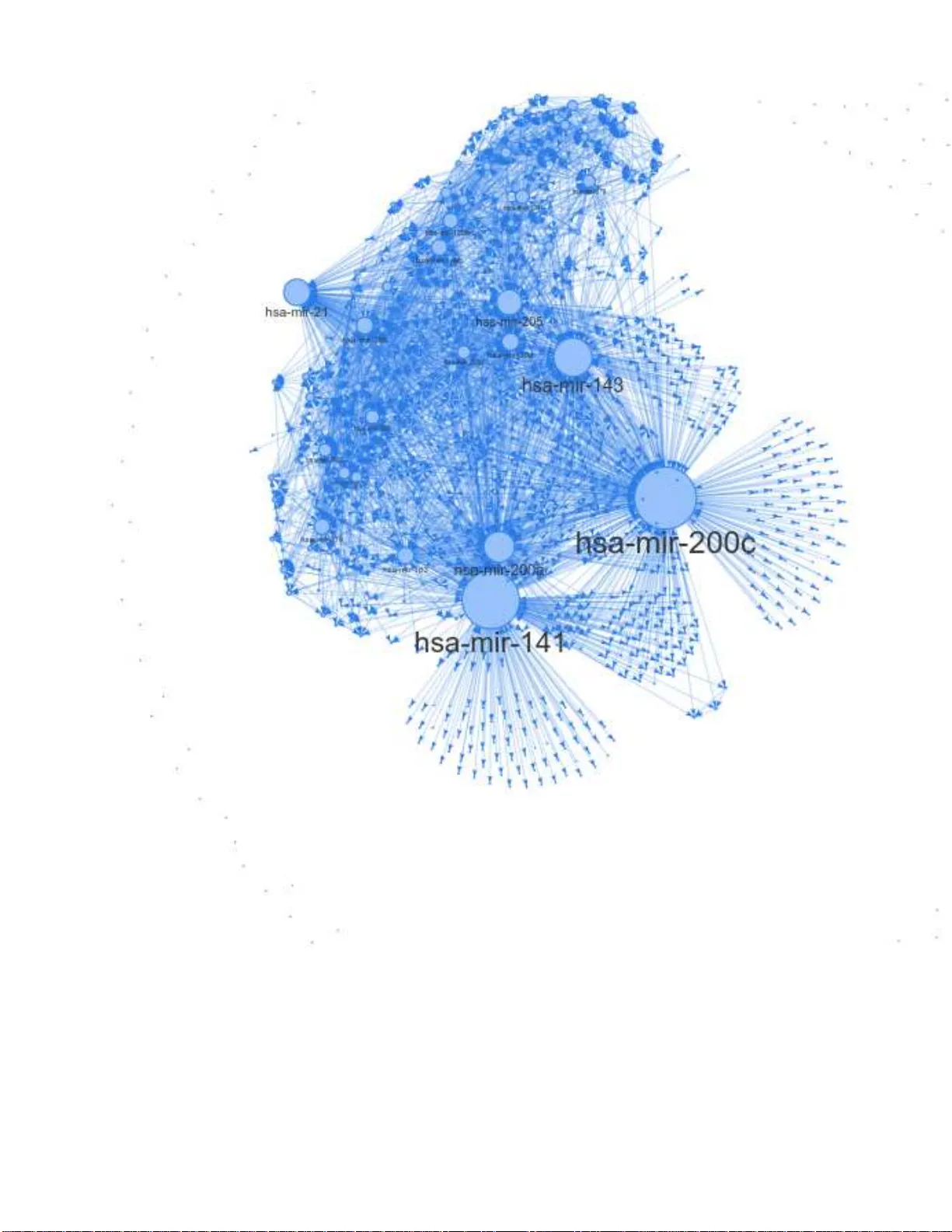
Interaction Networks fr om Discrete Ev ent Data by Poisson Multiv ariate Mutual Information Estimation and Inf ormation Flow with A pplications fr om Gene Expr ession Da ta Jeremie Fish, 1, 2 Jie Sun, 2 and Erik Bollt 1, 2 1 Department of Electrical and Computer Engineering Clarkson University 2 Clarkson Center for Complex Systems Science ∗ (Dated: Jul. 20, 2021) In this work, we introduce a new metho dology for inferring the interaction struc t ure of discrete va lued time series which are Poisson distributed. While most related methods are premised on continuo us state stochastic processes, in fact, discrete and counting eve nt oriented stochastic process are natural and common, so called time-point processes (TPP). An important application that we focus on here is gene exp ression. Nonparameteric methods such as the popular k-nearest neighbors ( KNN) are slow con v erging f or discrete processes, and thus data hungry . No w , with the ne w multi-v ariate Poisson estimator dev eloped here as the core computational engine, t he causation entrop y (CSE) principle, together with the associated greedy search algorithm optimal CSE (oCSE) allo ws us to efficiently infer the true n etwork structure f or t his class of stochastic processes that were pre viously not practical. W e illustrate the power of our method, first in benchm arking with synthetic datum, and t hen by inferring the genetic factors network from a breast cancer micro -R NA (miRN A) sequ ence count data set. W e show the Poisson oCSE gi ves the best performan ce among the tested methods anfmatlabd discov ers previou sly kno wn interactions on the breast cancer data set. ∗ fishja@cla rkson.edu 2 I. INTRODUCTION Understand ing the behavior of a com plex system req u ires knowledge of its u n derlyin g structure. However prior k nowledge of the network of interactions is often una vailable, necessitating estimation from da ta. Perhaps n o complex sy stem is more imp or- tant to our health and well being than Data-driven analysis of gene expression is a complex system that is es p ecially importan t to our health and well being. Howe ver, these data are generally time-p o int pro cess (TPP), and discretely distributed, r ather than continuo us valued as most mutual info rmation infe rence method s pr esume. Specifically , we assume a jointly distributed Poisson process. While TPP are relatively comm on, as far as we know , no efficient join t entropy estimato r e x ists. T o this end, the main goal of this pap er is to fill that gap. Granger causality [12] has be en u sed for network inferen c e when interpre te d as a causatio n inf erence co ncept, fo r linea r stochastic pr ocesses, as well as tr ansfer entr o py (TE ) [13] based o n inf ormation theorety for nonlinear pro cesses. Howe verm when applied to a system with mo re than two factors, neither of these conc epts can distinguish direct versus indirect ef f e c ts or co-fou nders, and therefore th ey w ill tend to yield false positi ve conne ctions. T o th is end, we developed causation entropy (CSE) as a gen eralization o f tr a n sfer entropy [14, 15], th at e xp licitly d efines the inform ation flow b etween tw o factors, conditioned on tertiary intermediary f acto r s. This, together with a greedy s ear ch algorithm to constru ct the network of interac tions o f the com- plex stochastic p rocess, p rovably r ev eals ne twork structure of certain sto c h astic pr o cesses, [15]. In p ast studies, TE as we ll as CSE were c o mputed n o nparam etrically , by the Kraskov-Stögba uer-Grassberger (KSG) [ 16] m utual inform ation estimator wh ich is a K-nearest neighb ors ( KNN) method. Howe ver, if specific knowledge o f the joint distribution of the p rocess allows consid- erable compu tation ef ficiencies, such as our previous work wher e join tly Gau ssian variables [15] or jointly Lap lace distributed variables in [17] we re r e levant. Here, we focus on gen e expression network s, which are an application of con siderable scientific importanc e due to the ir found ational relev anc e as a building b lock tool to understan ding d etails o f life science. It is well understoo d that many diseases associate with variations of the expression of a single gene [1 – 3], e.g ., famously such as sickle c ell disease and cystic fibrosis. Howe ver it rem ains a d ifficult p roblem with considerable h ealth im plications to explain and to in fer c omplex interac tio ns and associations when many genes may b e inv olved in co mmon and e ven de a dly disease. Such diseases are called poly genetic, and these includ e the breast cancer example that we stud y here. According to the Centers fo r Disease Contr ol (CDC), in the USA, brea st cancer is con sidered to be the second most comm o n f o rm of cancer amon gst woman, [4], that in 2019 was forecast to 268,600 cases and 42,26 0 death s in 20 19. W e advance here a new m e thodolo gy to pro b e variations in expr ession o f a gro up (network) o f gen es that may lead to d isease. Understand ing the gene interactio n n etwork stru c tu re may b e crucial to the development of f uture treatments. Ne twork inf e rence itself has many applications beyond cancer research, including fMRI network inference [5 – 8], drug-target interaction networks [9], and earthquake network inference [10 ] and econo m y issues [11] to n a m e a few . W ith this motiv ation , the m ain tec h nical pr emise of this paper is to develop a compu tationally efficient approa c h to estimate joint entropy and related infor mation theoretic measures for multiv ariate Poisson processes. Da ta deriv ed from these are discre te- valued data, and typically consist o f a sign ifican t fraction of zer os punctu ated with nonzero values describ in g event cou nts in a given ep och. From the multi-variate Poisson m odel, we derive an analytical series rep resentation of th e joint entr opy and the mutual info rmation. Then , a practica l finite partial-sum estimator allows estimation of mutua l info rmation, tow ard tran sfer entropy an d causation entropy . This paper is structured as follows: first, we provid e a b rief introdu ction to math ematical back groun d including a multivari- ate Poisson mod el and also r elev ant inform ation theoretic quantities which are necessary to define in formatio n flow . Then, we derived our mu ltiv ariate Poisson jo in t entr opy estimator, which we relate to n etwork infere n ce. Finally , in the Results section we dem onstrate our method and performance fo r bench mark sy n thetic data and then we study th e breast cancer gen e expression data sets. 3 M u l t i v a r i a t e P o i ss o n M o d e l f ( x 1 , …, x n ; { λ ij }) J o i n t P o i ss o n En t r o p y H ps ( X 1 , …, X n ; { λ ij }) A p p r o x i m a t e J o i n t P o i ss o n En t r o p y H ′ ps ( X 1 , …, X n ; { λ ij }) D i sc r e t e - v a l u e d M u l t i v a r i a t e D a t a { x i ( t )} i =1,…, n ; t =1,2,… parameter estimation analytical computation truncation Figure 1. W ork flo w of our computationally ef ficient approach t o estimate t he joint entropy of multi -v ariate Poisson distributed variables. From data, we proceed to distribution parameter estimation to approximate joint entropy . II. B A CKGROUND A. Multiva riate Poisson Model First let us reca ll the sing le variate Poisson Model, [18, 19]: p ( k ) = λ k k ! e − λ . (1) The P o isson mo del has a multivariate gene ralization as follo ws, [20]: P ( X 1 = x 1 , ..., X n = x n ) = (2) e − n P i =1 P j ≥ i λ ij X C n Q i =1 λ ( x i − P j a ij ) ii n Q i =1 Q j >i λ a ij ij n Q i =1 ( x i − P j a ij )! n Q i =1 Q j >i a ij ! , where the set C = (3) { A = [ a ij ] n × n | a ij ∈ N 0 , a ii = 0 , a ij = a j i ≥ 0 , X j a ij ≤ x i } , and N 0 = N ∪ { 0 } . This mo del is based o n a ssum ing that the x i are linearly transfo rmed from a set o f ind epende ntly drawn Poisson variables. W e begin with X ∈ N n × t 0 = ( x 1 , x 2 , ...x n ) T = B Y , (4) Y ∈ N m × t 0 = ( y 11 , y 22 , ..., y nn , y 12 , y 13 , ..., y ( n − 1) n ) T . Here each y ij is indep e ndent Poisson, that is: y ij ∈ N t 0 ∼ Poisson ( λ ij ) , ( fo r i = 1 , ..., n, j ≥ i ) , so m = n + n ( n − 1) 2 , B ∈ N n × m 0 . Note that in this case λ ij = λ j i . The rows of X thus rep resent Poisson ran dom variables which have t o bservations. Although the n umber of param eters needed to sp e cify this mod el grows quickly , th e re are some nice prop erties. For instance, this mo d el allows a si m ple estimate of each λ ij , since th e sum of indepen dent Poisson v ariables y ields the following covariance 4 matrix structure: Cov ( X ) =            λ 11 + n P j 6 =1 λ 1 j λ 12 · · · λ 1 n λ 12 λ 22 + n P j 6 =2 · · · λ 2 n . . . . . . · · · . . . λ n 1 λ n 2 · · · λ nn + n − 1 P j =1 λ nj            (5) with λ ij = λ j i . The ( i, j ) entries of the covariance matrix repr e sent cov ( x i , x j ) , the cov ar iance between the two rando m variables, x i and x j ) . Proo f of Eq. 5 may be found in the appen dix. This model is a m u ltiv ariate extension o f the Poisson mo del th at doe s not assum e the random variables are necessarily in- depend ent. Howe ver , there are some limitations to this mo del. First, th e rapid growth in the nu m ber of states an d pa r ameters with respect to the n umber of variables, making calculatio n of the jo int distribution co mputation ally unwieldy an d expensive. Another limitation is that mo del cannot handle negativ e covariance [20]. These difficulties are particularly complicating in the forth co ming en tropy com putations, and s o they must be handled in later sections. B. T ransfer Entropy and Causation En tropy W e briefly r evie w certain Shann on entrop ies, b u ilding tow ar d the con cepts of transfer entro py and causation entr o py . These are the fun damental co ncepts of info r mation flow we use to consider network inference . The Shanno n entr opy of a (discrete) random variable X is gi ven by [2 2, 2 3]: H ( X ) = − X x ∈ X P ( x ) log ( P ( x )) , (6) where P ( x ) is the probability that X = x , and 0 lo g (0) = 0 is th e usual interp retation in this co ntext. For the remainder of this pape r we choose the natura l log an d thus all e n tropies will be me a sured in nats. Entr o py can be th o ught of as a me a sure of h ow u ncertain we are abou t a particular outcom e. As an example we can imagin e two scenario s, in one ca se we ha ve a random variable X 1 = ( x (1) 1 , x (2) 1 , ..., x ( n ) 1 ) with x ( t ) 1 = 0( ∀ t ) , th at is P ( X 1 = 0) = 1 , in the other case the r a ndom variable X 2 = ( x (1) 2 , x (2) 2 , ..., x ( n ) 2 ) with P ( X 2 = 0 ) = 0 . 5 , P ( X 2 = 1 ) = 0 . 5 . Her e H ( X 1 ) = 0 nats, while H ( X 2 ) = ln (0 . 5) nats which happens to be the maximum for this case [23]. It is easy to see that Shan non entropy reaches it’ s greatest v alue when we are th e most uncertain abo ut the o utcome, and its minimal value ( 0 ) when we are co mpletely ce rtain abo u t the outcome. W e can now examine the case of tw o random variables X and Y . The joint entr opy of a discrete random v ariable is defined [ 2 3]: H ( X , Y ) = − X x ∈ X X y ∈ Y P ( x, y ) ln ( P ( x, y )) . (7) When th e two ra ndom variables X and Y ar e indepen dent H ( X, Y ) = H ( X ) + H ( Y ) which is the max im um joint entro py . Thus H ( X , Y ) ≤ H ( X ) + H ( Y ) . There are compa r able definitions of differential entropies for co ntinuou s random v ariables in term s of integration . The conditional entr opy is defined : H ( X | Y ) = − X x ∈ X X y ∈ Y P ( x, y ) ln P ( x | y ) . (8) The conditional entropy gi ves us a way to d escribe the relation ship between v ar iables, which is th e k ey to network inference. If knowledge o f the v ariable Y gi ves us complete k nowledge o f the variable X th en the conditional entropy will be H ( X | Y ) = 0 nats. Another important Shann on entropy is the mutu a l information which is defined as [23]: I ( X , Y ) = X x ∈ X X y ∈ Y P ( x, y ) ln  P ( x, y ) P ( x ) P ( y )  = H ( X ) − H ( X | Y ) = H ( X ) + H ( Y ) − H ( X , Y ) . (9) 5 Finally , the K ullback-Leibler ( KL) diver gence ( D K L ) [23 ] is stated : D K L ( P || Q ) = − X x ∈ X P ( x ) ln  Q ( x ) P ( x )  . (10) The KL diver g ence descr ibes a distance-like q uantity be tween two probability distributions, though it is not a metric as for on e, it is n o t symmetric (that is in g eneral D K L ( P || Q ) 6 = D K L ( Q || P ) ), and also it does no t satisfy the triang le inequality . Mutual informa tio n E q. 9 can be written in term s of KL d ivergence as [23]: I ( X , Y ) = D K L ( P ( x, y ) || P ( x ) P ( y )) , (11) describing a de v iation from in depend ence of a joint r andom v ar iab le ( x, y ) . For a stationary stoc hastic process, { X t } , the entr opy r ate is defined as [37, 3 8]: H ( χ ) = lim t →∞ H ( X t | X t − 1 , X t − 2 , ...X 1 ) . (12) If th e pr ocess is Markov (m emory less) then [23]: H ( χ ) = lim t →∞ H ( X t | X t − 1 ) . (13) The t ransfer entr op y from X 2 to X 1 is d efined [1 3, 14]: T X 2 → X 1 = H ( X t +1 1 | X t 1 ) − H ( X t +1 1 | X t 1 , X t 2 ) . (14) Causation en tr opy is a generaliza tio n o f th e tran sfer entro py , wher e [1 4, 15]: C Q→P |S = H ( P t +1 |S t ) − H ( P t +1 |S t , Q t ) . (15) C Q→P |S is designed to describ e the remaining information flow from processes Q to processes P th at may not acco unted for H(X) H(Y) H(Z) H(X|Y,Z) H(Y|X,Z) H(Z|X,Y) C Z  Y|X (a) (b) H(X) H(Y) H(Z) H(X|Y,Z) H(Y|X,Z) H(Z|X,Y) Figure 2. (a) The causation entropy between t wo processes Z and Y is sho wn. In this case sinc e we are only conditioning on a process X , C Z → Y | X = T Z → Y . Of course X may be replaced with a set of v ariables. (b) Here we sho w a special case where Z is independent of both X and Y ( Z in this case may represent the history of X . In this case it bec omes clear that H ( Z | X, Y ) = H ( Z ) , H ( X | Y , Z ) = H ( X | Y ) and H ( Y | X, Z ) = H ( Y | X ) . As explained in the text, this special case helps us to discern what are the proper variables to use in the Poisson case. (conditio ned on ) p rocesses S . An example o f ca usation entr opy is sho wn in Fig. 2 (a). In theory if a process Z has no influence over another proc e ss Y , th e causation en tropy after condition ing out the re maining pro cesses would be id entically 0 , a llowing us to r eject a conn ection from Z to Y . In p ractice h owe ver, when estima tin g th ese qu antities by statistics fr om finite sam p les of noisy data, these will no t compu te to be identically 0 , making it necessary to have a threshold, which is the pu rpose of using a shuffle test a s d iscussed in [15]. Network inferen ce can be developed based on Eq. (15). Ho wever , considering the power -set o f all po ssible subsets P , Q , S is clearly NP-h ard and so not p r actical. Th is led to the development of a g reedy sear ch alg o rithm, we r eferred to as optimal 6 causation entropy (oCSE) [15, 17] to a m in imal network that explains the data, in terms of minim a l causation entropy . T his proceed s in two stages, agg regativ e disco very of statistically significant links, those that are maximally informa ti ve influencers in term s of th e co n ditionally already sig n ificant links, with possible removal o f statistically irrelev ant links de velope d while growing the g lobal network, and significance decid ed by a nu ll h ypoth esis in ter ms of mu ltiple random shuffles o f the data. W e wer e able to prove under mild hypoth esis of the stochastic p rocess that this procedu re will discover the true network, also assuming a good statistical estimation of the en tropies. It is p recisely this p roblem of good data-driven statistical estimation of en tropies specialized to the scenario of a multiv ariate Poisson process which is what we ha ndle in this pap er in the case o f multiv ariate Po isson. III. ENTR OPY ESTIMA TION FROM MUL TIV ARIA TE POIS SON DA T A A. Estimating Joint Entropy of Poisson Systems Here we d evelop an estima tor of en tropies for the multiv ariate Poisson d istribution, Eq. ( 2). T o this end, we trunca te partial sums fr om s er ies repr esentations. B. Poisson Entropy W e b egin the Poisson Entro py: H P oisson ( K ) = − ∞ X k =0 λ k k ! e − λ ln  λ k k ! e − λ  = (16) − ∞ X k =0 λ k k ! e − λ [ − λ + k ln ( λ ) − ln ( k !)] = λ − λ ln ( λ ) + ∞ X k =0 λ k k ! e − λ ln ( k !) . This expression for th e entropy of a Poisson rando m v ariable is in terms o f an infinite series, which is well approx imated by a finite tru ncation p artial sum . C. Biva riate Poisson Entropy The B ivariate Po isson case is instru ctiv e to the n- variate Poisson case. Con sid er: P ( x 1 , x 2 ) = e − λ 11 − λ 22 − λ 12 λ 11 x 1 x 1 ! λ 22 x 2 x 2 !  min ( x 1 ,x 2 ) X a 12 =0 x 1 ! ( x 1 − a 12 )! x 2 ! ( x 2 − a 12 )! a 12 !  λ 12 λ 11 λ 22  a 12  . (17) Let, d 12 = λ 12 λ 11 λ 22 , (18) and, D ( x 1 , x 2 ) = min ( x 1 ,x 2 ) X a 12 =0 x 1 ! ( x 1 − a 12 )! x 2 ! ( x 2 − a 12 )! d a 12 12 a 12 ! . (19) Then Eq . 17 will become : P ( x 1 , x 2 ) = e − λ 11 − λ 22 − λ 12 λ 11 x 1 x 1 ! λ 22 x 2 x 2 ! D ( x 1 , x 2 ) . (20) Now to get the jo int en tropy of the Biv ariate Poisson we h av e: 7 H ( X 1 , X 2 ) = − ∞ X x 1 =0 ∞ X x 2 =0 P ( x 1 , x 2 ) ln ( P ( x 1 , x 2 )) = − ∞ X x 1 =0 ∞ X x 2 =0 e − λ 11 − λ 22 − λ 12 λ 11 x 1 x 1 ! λ 22 x 2 x 2 ! D ( x 1 , x 2 )[ − λ 11 − λ 22 − λ 12 + x 1 ln ( λ 11 ) + x 2 ln ( λ 22 ) − ln ( x 1 !) − ln ( x 2 !) + ln ( D ( x 1 , x 2 ))] . (21) A s cen ario of interest arises when λ 11 , λ 22 , and λ 12 are all small and λ 12 << λ 11 λ 22 . . In this case we have D ( x 1 , x 2 ) ≈ min ( x 1 ,x 2 ) X a 12 =0 d a 12 12 a 12 ! , (22) since the d 12 term dom inates. Sm a ll λ 11 and λ 22 ensures that th e large x 1 and x 2 terms to become insignificant in Eq. 21. Thus, D ( x 1 , x 2 ) ≈ 1 + d 2 12 2! + ... ≈ 1 . Grou ping ter m s and rem embering (th e middle part of) Eq. 16, and estimating D ( x 1 , x 2 ) = 1 , a finite p artial sum of Eq . 21 can be written: H ( X 1 , X 2 ) = e − λ 12 [ H ( X 1 ) + H ( X 2 ) + λ 12 ] . (23) Rememberin g th e assumption λ 12 << 1 , th e e xp ression Eq. 23 reduces fur ther: H ( X 1 , X 2 ) = [ H ( X 1 ) + H ( X 2 ) + λ 12 ] . (24) As Fig . 3 shows, this ap proxim ation works well when d 12 << 1 = ⇒ λ 12 << λ 11 λ 22 , and in this regime the error will be small. Similar analy sis can be carried out for the larger m u ltiv ariate cases which allo ws us to arriv e at a general fo rmula fo r our approx imation g iv en by: H ( X 1 , X 2 , ..., X n ) ≈ [ H ( X 1 ) + ...H ( X n ) + X j >i λ ij ] , (25) where we are assuming that λ ij are small for all ( i, j ) p airs. Fortun ately as we can see in Eq. 25, all of the qu antities o n th e r ig ht hand side are computatio nally efficient to com pute. This in f act greatly r e duces the computational time necessary f or estimation of the joint entropy . This form ulation req uires asymptotic assumptions that may not b e valid in gen eral in nature. Ho wever we find empir ically in simulations th at by scaling the rates λ ij to b e in [0 , 1 ] the esti m ate per forms well, as described by Fig. 3 and, verified in the network simu lations, regard less o f wh at the true un d erlying rates this scaling produces similar r esults. As a note of caution, consider that when calculating the mutual information in the Poisson model, care must be taken due to h ow th e marginals of a join t Poisson process are drawn. For examp le from Eq. 9 it may be tempting to assert: I P oisson ( X 1 , X 2 ) = H ( X 1 ) + H ( X 2 ) − H ( X 1 , X 2 ) , (26) with X 1 ∼ Poisson ( λ 11 ) and X 2 ∼ Poisson ( λ 22 ) . Howev er this is n o t exactly correct, tho ugh the err or here is subtle. I n fact we must make a small chan g e to Eq. 26 to be: I P oisson ( X 1 , X 2 ) = H ( ˆ X 1 ) + H ( ˆ X 2 ) − H ( X 1 , X 2 ) , (27) here X 1 ∼ Poisson ( λ 11 ) and X 2 ∼ Poisson ( λ 22 ) , but ˆ X 1 ∼ Poisson ( λ 11 + λ 12 ) and ˆ X 2 ∼ Poisson ( λ 22 + λ 12 ) . This subtle d ifference is imp ortant, beca u se without reco gnizing this fact, th e calcu la te d mutua l inform ation becomes negative, which violates our well estab lished co ndition th at mu tual inf ormation be p ositiv e. The need fo r ˆ X 1 and ˆ X 2 is appar e nt fr om E q. 5, when two Poisson ran dom v ariab les are summed tog ether their mar gina ls then are drawn from the sum of the underly ing rate (i.e. λ ii ) and the cou pling rate (i.e. λ ij ). Th is also transfers to comp uting the condition al mutual info rmation. T o b etter illuminate this calculation it is helpful to refer to Fig. 2 (b). I ( X , Y | Z ) = H ( X , Z ) + H ( Y , Z ) − H ( X , Y , Z ) − H ( Z ) . (28) In th e specia l case pr esented in Fig. 2 ( b) Eq. 3 7 b ecomes I ( X , Y | Z ) = I ( X , Y ) = H ( X ) + H ( Y ) − H ( X , Y ) , (29) therefor e, H ( X ) + H ( Y ) − H ( X , Y ) = H ( X , Z ) + H ( Y , Z ) − H ( X , Y , Z ) − H ( Z ) . (30) 8 In th is s p e cial case we can note the follo win g: H ( Y , Z ) = H ( Y ) + H ( Z ) . (31) Applying Eq . 31 to Eq. 30 we find that: H ( X ) − H ( X , Y ) = H ( X , Z ) − H ( X , Y , Z ) . (32) W e k now from Eq. 27 that in the Poiss o n case this beco mes: H ( ˆ X ) − H ( X , Y ) = H ( X , Z ) − H ( X , Y , Z ) . (33) Applying the following facts to Eq. 33 ( H ( X , Y , Z ) = H ( X , Y ) + H ( Z ) , and H ( X, Z ) = H ( X ) + H ( Z ) , (34) we find that: H ( ˆ X ) = H ( X ) . (35) Similar an alysis also shows that: H ( ˆ Y ) = H ( Y ) , (36) this im plies that we must use the Poisson marginals in the co m putation of th e con ditional mu tual inform ation. That is in the Poisson ca se we mu st h av e: I ( X , Y | Z ) = H ( ˆ X , Z ) + H ( ˆ Y , Z ) − H ( X , Y , Z ) − H ( Z ) . (37) Note the use o f ˆ X and ˆ Y in this case. This distinc tio n in the Poisson case is importan t because we note that witho ut using the proper m arginals the comp utation results in negative con d itional m utual inf ormation which is clear ly not correct since con ditional mutual inf ormation mu st be positiv e [ 23]. Impor tan tly the new definition giv en in Eq. 25 becom es more co mputation ally efficient than comp uting the Poisson jo int entropy directly fro m the joint pro b ability . This requ ires calculation of only separ ate single variate entropies which is r equires less computation . This naturally lead s to the qu estion o f the accur acy of th is n ew mo del. As can be seen in Fig. 4 the new definition o f en tropy still lead s to accurate id entification o f network structure. This new defin ition also fits into the gen eral framework of entropy which was de velope d ab ove, allowing us to apply the oMII algorithm to the d ata. D. Network Stru cture and Inference In a gen e interaction n etwork, un d erstanding how future trea tm ents could be d eveloped, especially in the cases where more than a single gene may b e implicated in a d isease, may help in d esigning targeted fo r th erapies. Gen e s inter a c t with outcome such as d isease redu ces to a n etwork inference problem . W e do n ot assum e apr iori knowledge of the und erlying network structu re, but i n stead we have data describ ing time series o f e volving stochastic processes at each of the states, related to each indi v id ual gene. Th e network is stated as a g raph G defin ed as a set of vertices V ⊂ N and edges E ⊂ V × V , G = {V , E } . Note that |V | = n denotes that there are n v ertices (or nodes) in G , by the c ardinality , | · | , of a set. The adjacency ma tr ix A ∈ N n × n 0 is a conv en ient way to encode a graph , ( A ij = 1 if ( i, j ) ∈ E , A ij = 0 otherwise . (38) When a system has a graph struc tu re it is often refer red to as a n etwork. The adjacency ma trix then enc odes the network structu re of the system. Our go a l is to estimate network structure ˆ A closely as possible to the true network structure A , that is we want, P i,j |A − ˆ A| , to be as small as po ssible ( ideally 0 ). W e would also like for th is to be acco mplished with as little d ata ( t ) as possible, since we are often limited in the amount of real world data we receive. Our estimation of the network structure relies on no d es sharing info rmation with o ne anoth er . Thu s ˆ A may be th ough t of as whic h nodes are directly communicating with one another, rath er than strictly being the physical stru cture. In our previous w ork , [14, 15], we proved that un der mild hypothesis, 9 Figure 3. T he relativ e error in the j oint entropy calculation between the joint entropy calculated through truncation and the joint entropy calculated by our approximation. It is clear that when both λ 12 and λ 11 λ 22 are small, the relativ e error is small. Thus we expect this approximation to work well when all of the estimated r at es are small. In practice we fi nd that when scaling the rates to be in [0 , 1] we get good results, regardless of how high t he t r ue rates were. the multi-variate stochastic ev olvin g by coup ling on a complex network can be derived perfectly by optimal causation entro py (oCSE), errors a r ising f rom estimatio n issues such as model e ntropies o f o b servations f rom various distributions, an d finite data effects, but the in formatio n n etwork structur e align accurately in most situa tio ns. In the first example demo nstration of ou r metho ds, we benchm ark with syn th etic simulated by the multivariate Poisson model, Eqs. 2 - 4. T o explicitly in c orpor ate the adjacency matrix A and n oise E as shown in [24, 26], consider as: X = B Y + E , (39) B = [ I n ; P ⊙ (1 n tri ( A ) T )] (40) where I n is the ( n × n ) identity matrix, P ∈ N n × ( m − n ) 0 is a permutatio n matrix with e xa c tly n ones per row ⊙ represents the Hadamard pro duct (comp o nentwise mu ltiplication of same sized ar rays). 1 n ∈ N n × 1 is the vector o f all on es, and tri ( A ) ∈ N n ( n − 1) 2 × 1 0 denotes the vectorized upper triangular portion of the adjacen cy matrix, and E ∈ N n × t 0 . W e have established in previous discussion that there is no analytical solutio n for the en tropy of the multivariate Poisson, instead a n ap proxim ation has been made. Sin c e the Poisson distribution resemb les th e Gau ssian distrib ution often the latter is assumed for estimates, we thus compare the perfor m ance of oMII assuming b oth d istribution types. Fig. 4 shows that the oMII method , but even u sing the rough Gau ssian best estima te s o f e n tropies, n onetheless d oes r e asonably well find ing the true edg es with a hig h true positive rate (TPR). Th is is contrasted to n etwork inferen ce based on oth er entr opy estimators, includin g the nonparam etric k NN meth o d, GLASSO, both of which are discu ssed belo w , an d a lso the Poisson estima to r d eveloped here. Howe ver , the Gaussian o MII finds the edges at the expe nse of a m uch larger false po siti ve rate (FPR). Specifically , d efine TPR an d FPR as follo ws: let G = {V , E } be th e tru e network structure and ˆ G = { ˆ V , ˆ E } be the estimated n etwork structur e. Th en: TPR = |E ∩ ˆ E | |E | , (41 ) and FPR = | ˆ E \ E | |E | . (42) In th is case \ represents set subtraction. No te that from th is d efinition 0 ≤ TPR ≤ 1 wh ile FPR ≥ 0 . IV . RESUL TS W e comp are the p erform ance of sev er a l meth ods on simulated da ta sets, including various ty p es of oMII, as well as GLASSO [25]. Unlike oMII, w h ich inv olves condition al mutual info r mation as its engine, GLASSO in volves maximizin g the log- 10 likelihood pr ovided in Eq. 43 o ver values o f a regularizatio n p arameter ρ , L ( X, ρ ) = lo g ( det ( ˆ A )) − trace ( Cov ( X ) ˆ A ) − ρ || ˆ A|| 1 . (43) A com mon m ethod for the cho ic e of ρ is maximazation of the Bay esian infor mation cr iterion (BIC). W e utilize 1000 log-space d values o f ρ in [10 − 2 , 1 ] which varies ˆ A between a com plete n etwork to a completely disconnected n etwork with zero edges. Follo win g [2 6], first we use a box-cox transform ation of the P o isson d istributed data, to make the data mo re Ga u ssian like, pr ior to u sin g GLASSO. The box-cox tran sformation of a rand om variable z is bc ( z | γ ) = ( z γ − 1 γ if γ 6 = 0 log ( z ) if γ = 0 . (44) GLASSO results ar e shown in Fig. 4. The Poisson oMII m ethod is tested on d ata simu la te d as describ e d in the section ab ove. In Fig. 4 each d ata p oint is averaged over 50 realiza tions of the n etwork dyn amics. T wo different Erd ˝ os-Rényi (ER) graph types are used, one with p = 0 . 04 and one with p = 0 . 1 . The par a m eter p in an ER grap h contr ols the sparsity of the g raph, th us the g raphs with p = 0 . 1 will have considerab ly mo re ed ges on average tha n grap h s with p = 0 . 04 . For th ese simu lations n = 50 was chosen. The rates were chosen to be λ ij = 1 ( ∀ i, j ) and E i ∼ Poisson (0 . 5) ( ∀ i ) where E i ∈ N t × 1 0 are the column s of E . This is th e high SNR scenario from [2 4]. T o estimate the rates, we simp ly use cor relation b etween all pairs in the data. W e note that this dif fer s fro m above where we utilized the co variance matrix. Using correlation rather than co variance guarantees the calculated rates will be relativ ely small since the values o f co rrelation d o not exceed 1 in a b solute value, this allows the estimated rates to stay in the small relati ve error re gim e shown in Fig. 3. Th e correlation m atrix then gi ves us all of the of f diagonal rates λ ij ( i 6 = j ) and to obtain the rates λ ij ( i = j ) we can see fr om Eq. 5 tha t w e simply need to subtract the sum of the non-d iagonal elements from the d iagonal elem ents. That is if we let Corr ( X ) =     e 11 λ 12 · · · λ 1 n λ 12 e 22 · · · λ 2 n . . . . . . · · · . . . λ n 1 λ n 2 · · · e nn     , (45) then λ ii = e ii − P j 6 = i λ ij . In Fig. 4 it can be seen that in terms of TPR all of the metho d s perform quite well with the exception of the KNN v ersio n o f oMII which e xh ibits po or perfo rmance acro ss all e x amined sample sizes, likely d ue to slow conv ergen ce. In fact, fo r ne tworks with few c onnectio n s the poor est per f orming meth od in term s o f TPR is the Poisson o MII method, w ith the best p erform ing method being GLASSO. Howe ver GLASSO produ ces a very high FPR, in fact GLASSO finds mo r e false positives than there a r e total ed ges in the true network, th us producin g an FPR of greater than 1 . By co n trast bo th Gau ssian and Poiss o n versions of oMII p roduce s ig nificantly lo wer FPR a nd the Poisson oMII produces the lo west rate of FPR across all sample sizes. It should be n oted as well that the FPR o f the Poisson version of o MII maintains an app roximately co nstant le vel across all samp le sizes, while the Gau ssian versio n o f oMII has an in creasing FPR with sample size. For the d enser network s, which had an expected average degree of 5 , as expected all meth ods had a d ecreased TPR for low sample size. The FPR also fell fo r all methods d u e to the larger de n ominato r (mor e edges). T he conc lusions remain the same for both network d ensities. W e n ow examin e data derived from breast cancer p atients who have been screened for d ifferent micro RN A ’ s (miRN A ’ s) occurre n ce coun ts of is analy zed b y th e Poisson oMII metho d f eatured in this pa p er . T hese data sets are pub licly available at https://portal.g dc.cancer .g ov website, described as TCGA-BRCA seq uencing miRN A. In this case, t = 1 207 an d n = 1881 different miRNA samp les are available. Of these, 1881 m iRN A ’ s ≈ 100 0 p ass the two sample K olmo gorov-Smir nov (KS) [30] test comp aring to the Poisson d istribution, to confidence level α = 0 . 05 . The r emaining ≈ 900 miRN A data were then scaled as follows: x ∗ i ∈ N 1207 × 1 0 = ⌊ x i < x i > ⌋ . (46) The notation, < · > represen ts the mean an d ⌊·⌋ compo n entwise, to integers. The scaled da ta is well fitting, ag ain by KS-test, to a n egati ve binomial distribution, with on ly ≈ 200 failing as b oth Poisson and negati ve b inomial. Recall that the Poisson distribution is a special c a se o f th e negative binom ial distribution, since: P N eg B in ( k ) =  k + r − 1 k  λ k (1 − λ ) r . (47) In the limit, r → ∞ in Eq. 47 it is ea sy to see that the term (1 − λ ) r → e − λ , and rewriting  k + r − 1 k  = ( k + r − 1)! k !( r − 1)! → 1 k ! . Combining these facts, as r → ∞ , the negative binom ial distribution limits to a Poiss o n d istribution. 11 0 200 400 600 800 1000 Sample Size (T) 0 0.2 0.4 0.6 0.8 1 TPR (a) 0 200 400 600 800 1000 Sample Size (T) 0 0.5 1 1.5 2 2.5 FPR (b) Poisson ER 0.04 Gaussian ER 0.04 KNN ER 0.04 GLASSO ER 0.04 Poisson ER 0.1 Gaussian ER 0.1 KNN ER 0.1 GLASSO ER 0.1 0 200 400 600 800 1000 Sample Size (T) 0 0.2 0.4 0.6 0.8 1 TPR (c) GLASSO Hybrid Poisson 0 100 200 300 400 500 600 700 800 900 1000 Sample Size (T) 0 0.1 0.2 0.3 0.4 0.5 0.6 0.7 0.8 FPR (d) Figure 4 . True P ositiv e and False Positi ve R ates f or several test methods on ER graph s of two different levels of sparsity . Erd ˝ os-Rényi (ER) graphs with tr i angles for a 50 nodes graph with strong sparsity due to p = 0 . 04 , and the x’ s for 50 nodes ER graphs with due t o denser p = 0 . 1 . The magenta li nes represent GLASS O, the blue lines represent t he Poisson oMII, the red lines r epresent the Gaussian oMII, and the green lines represent the KNN oMII. In (a) the true positiv e rate (TPR) is shown for dif ferent sample sizes, each point is averag ed o ver 50 realizations of the network dynamics. In (b) the false positiv e rate (FP R) is shown. Clearly GLASS O finds more true edges, but at the expe nse of a significantly higher false positiv es. In fact, for the highly sparse ER network GLASSO finds 3 times as many edges as actually exist in the network with 1000 data points. T he F PR increases with data set. As c an be seen the Gaussian oMII pe rforms as well as Poisson oMII in TP R with the KNN performing poorly , but the Poisson oMII significantly outperforms all other methods in t erms of FP R. It appears t hat the Poisson oMII is the only method tha t co nv erges to the true network structure with increasing sample size. (c) Comparing TPR between GLAS SO, the hybrid method a nd Poisson oCS E. The hyb rid method has an increased TPR relative to Poisson oCSE. (d) The FP R increases slightly for t he hybrid method, but is substantially lo wer than GL ASSO. Giv en that the major ity of this miRN A data is distributed as scaled negative binomial (the Poisson data a lso can be fit as negativ e b inomial) we must interp ret the results of with caution esp e cially in light of the results sh own in Fig. 4. The results of the a pplication of the Poisson oMII still a re interesting , especially in light of the fact that the negative binom ia l distribution can be viewed as a compound Po isson d istribution [27, 2 8]. T o obtain the n etworks shown in Fig. 5 we first restricted th e data to h aving a minimum of > 100 tota l counts,this w as to a void includ ing data that ha d zero variation o r n ear z e ro variation. This restriction left us with 1 072 m iRN A ’ s, oMII was then used to analyze the remaining m iRN A data without any fur ther pre-processing , which resulted in the network shown in Fig. 5. The n etwork h a s m any miRNA ’ s which are no n-interactin g, h owe ver there is a large weakly connec ted comp onent. Focusing on the n o des wh ich ar e mem bers o f the largest weakly con nected co mpon e n t (L WCC) we fou nd that many miRN A ’ s that have b een previously id entified as up or down regulated in br east cancer end up in this com ponen t, this component in cluded most of the miRN A ’ s listed in T ab le 1 of [29]. The miRN A ’ s which land in the L WCC will b e lab eled as inter esting m iRN A ’ s for brevity . Focusing on this set of 6 5 6 miRN A ’ s, th e plot of Fig. 5 focuses in o n this comp onent by sizing the nodes re lativ e to their out degree. Th e nodes with no out degre e are so small th at they are d ifficult to see in the figure, while th e nodes with largest out degree a re prom inent. A feature of this network is that ther e are miRN A ’ s th at are "driv ers" of th e n e twork , in that they have much larger out degree tha n the m ajority of other nod es. W e list the top 20 miRNA ’ s in o rder of their cen tr ality b a sed on ou t degree, betweenness centrality and eigen vector centrality in T able IV. For all three measures the top 4 miRN A ’ s are identically ordered , all 4 of which have b een noted f or a prominent role in breast cancer [29, 31 – 35] and they seem to be th e main dr iv ers. This suggests that it may be p ossible to target a small n umber of miRN A ’ s for some desired beha v ior of the system of miRN A ’ s in d r ug development. 12 Out Degree Betweenness Centrality Eigen vector Centrality Mir-200c Mir-200c Mir-200c Mir-141 Mir-141 Mir-141 Mir-143 Mir-143 Mir-143 Mir-200a Mir-200a Mir-200a Mir-21 Mir-205 Mir-205 Mir-205 Mir-21 Mir-21 Mir-30a Mir-26b Mir-30a Mir-26b Mir-30a Mir-183 Mir-183 Mir-183 Mir-26b Mir-199b Mir-199b Mir-326 Mir-210 Mir-125b -2 Mir-200b Mir-125b -2 Mir-134 Mir-210 Mir-134 Mir-326 Mir-125b -2 Mir-326 Mir-3607 Mir-199b Mir-200b Mir-379 Mir-429 Mir-379 Mir-210 Mir-32 Mir-3607 Mir-1976 Mir-3607 Mir 429 Mir-150 Mir-134 Mir-32 Mir-203a Mir-766 Mir-337 Mir-100 Mir-100 T able I. The top 20 genes discovered from the hybrid metho d in terms of: out de gree, betweenness c entralit y , and eigen vector centrality . All of these genes have been linked to breast cancer by p revious studies. 13 Figure 5. Example network generated by the hybrid oMII al gorithm. Nodes and text are si zed relativ e to t he out degree of t he node. The nodes with largest out degree have previo usly be en co nnected with breast cancer . 14 V . CONCLUS ION In this p aper we have given an appr o ximation to the mutual infor m ation of a mu ltiv ariate Poisson system. W e h av e shown throug h num e rical experimen ts that this ap proxim ation works ef ficiently , and the results of network estimation indicate that the approx imation is justified. W e ha ve also developed the oMII (and by extension the oCSE) algorith m for comp utation of the causation en tropy of a Poisson system based on the jo int en tropy approx imation discussed ab ove. W e have shown th a t this model is superior to simply assuming the d ata is Gaussian, which is likely related to the strang e behavior of th e marginals in a Poisson sytem, as we have outlined above. The Poisson oMII algorith m also significan tly ou tperfo r ms the nonparam e tric KNN version of oMII . Fina lly , we have applied the Poisson oMI I alg orithm to a b reast c a ncer miRN A expre ssion coun t dataset, which has prod uced potentially interesting insights into the network of m iRN A ’ s as it relates to breast cancer . Our network inferen ce on the breast can cer miRN A network has shown that there is a relationsh ip b e tween the hig hest variance (in expression values) of miRN A ’ s. There seems to be unidirection al conn ections between these miRN A ’ s, with certain miRN A ’ s taking on th e role of drivers in the network. This may su ggest a future course o f actio n for futu re dru g de velopm e nt. VI. ACK NO WL EDGEMENTS E.B. was supported by the Army Research Office (N6816 4-EG) and, J.F . and E . B. were supported b y DARP A. VII. APPENDIX Below we offer p roof of Eq. 5. Pr oof. Covariance of the multivariate Poisson In th e mo del presen ted in Eqs. 2, 3, 4, we can see that: x 1 = y 11 + y 12 + ... + y 1 n (48) x 2 = y 12 + y 22 + ... + y 2 n . . . x n = y 1 n + y 1 n + ... + y nn W ithout lo ss of ge nerality we will look a t the pair ( i = 1 , j = 2 ) . In this case we see that the covariance between this pair o f random variables is defined: cov ( x 1 , x 2 ) = E [ x 1 x 2 ] − E [ x 1 ] E [ x 2 ] , (49) Considering Eqs. 48, 49 and noting y 12 = y 21 , we h av e: cov ( x 1 , x 2 ) = E    y 2 12 + n X i =1 i 6 =2 n X j =2 y 1 i y 2 j    (50) − E [ y 11 + y 12 + ... + y 1 n ] E [ y 12 + y 22 + ... + y 2 n ] Because the expectation is a linear o perator,Eq. 50 can be expressed a s: cov ( x 1 , x 2 ) = E [ y 2 12 ] + E    n X i =1 i 6 =2 n X j =2 y 1 i y 2 j    − (51)    E [ y 12 ] + n X i =1 i 6 =2 E [ y 1 i ]      E [ y 12 ] + n X j =2 E [ y 2 j ]   . 15 From the in depend ence o f each y ij the covariance can thus be expr essed: cov ( x 1 , x 2 ) = E [ y 2 12 ] + n X i =1 i 6 =2 n X j =2 E [ y 1 i y 2 j ] − (52) E 2 [ y 12 ] − n X i =1 i 6 =2 n X j =2 E [ y 1 i y 2 j ] = E [ y 2 12 ] − E 2 [ y 12 ] = V ar ( y 12 ) . Since y 12 is independ ent Poisson and from the v ar ia n ce o f an independent Poisson ran dom v ariab le V ar ( y 12 ) = λ 12 . Applying this to ea c h i , j ( i 6 = j ) pair gives the desired covariance stru cture. [1] C. S Rogers, et. al. Disruption of t h e CFTR Gene Produces a Model of Cystic Fi b rosis i n Newborn Pigs Science 321, 1837-1841 (2008) [2] P . Sebastiani, M. F Ramoni, V . Nolan, C. T . Baldwin, M. H. Steinberg Genetic Dissection and Prognostic Modeling of Overt Stro ke in S ickle Cell An emia Natur e Gen eti cs 37, 435 (2005) [3] K. De Boulle, et. al. A Point Mutation in the FMR-1 Gene Associated with Fragile-X Mental Retardation Natur e Genetics 3, 31 (1993) [4] https://www .cdc.go v/cancer/breast/statistics/index.htm (2019) [5] S. M S mith Th e Fut u re of FM RI Connectivity Neur oimage 62, 1257-1266 ( 2012) [6] B. J. Stoltz, H. A. Harr i ngton, M. A. Porter P ersistent h omology of time-dependent functional networks constructed fr om cou pled t ime series C haos: An Interdisciplinary Journal of Nonlinear Science 27, 047410 (2017) [7] D. Bassett, et. al. Dynamic re configuration of human brain networks during l earning P N AS 108, 7641-764 6 (2011) [8] J. Fish, A. DeWitt, A. A. R. Almomani, P . J. Laurienti, E. Bollt E ntr opic re gression for neur ological motivated applications arxi v , (2021) [9] Y . Y amanishi, J. P . V ert , M. Kan ehisa Prediction of Drug-T arget Interaction Netw orks from t h e Integration o f Chemical and Ge- nomic Sp aces Bi oinformatics 21, i468-i477 (2008) [10] Y . Zhang, H. Zhao, X. He, F . D. Pei, G. G. Li Bayesian Prediction of Earthquake Network Based on Sp ace-Time In fluence Domain Physica A 445, 138-149 (2016) [11] G. Iori et. al A network analysis of the Italian over n ight money market Jou rnal of Economic Dynamics and Conr ol 32, 259-27 8 (2008) [12] C. W . G r anger In vestigating Causal Relations by Econometric Models and Cr oss-Spectral Methods Econometrica: Journa l of the Econometric Society 424-438, (1969) [13] T . Schreiber Measuring In for mation T ransfer Phys. Rev . Lett. 85, 461 (2000) [14] J. Sun, E. M . Bollt Cau sation Entropy Identifi es Indi rect Influ ences, Dominance of Neigbors and Anti cipatory Couplin gs P hysica D 267, 49 (2014) [15] J. Sun, D. T aylor , E. M. Bollt Ca u sal Network Inference b y Optimal Causation Entropy SIAM J. Appl. Dyn. Sys. 14, 73 (2015) [16] A. Kraskov , H. Stögbauer P . Grassberger Estimating Mutual In formation P hysical Review E 69, 066138 (2004) [17] A. S. A mbegedara, J. S un, K. Janoyan, E. M. Bollt Information Th eoretical Noninv asive Damage Detection in Brid ge Structures Chaos 26, 116312 (2016) [18] R.D. R eiss A course on point proc esses Springer Science (2012) [19] E. M. Bollt, N. Santiti ssadeek orn A pplied and Compu tational Measurable Dyn amics SIAM 2013 [20] D. Karlis, L . Meligotsidou Finite M ixtures of Mu l tiva riate Poisson Distributi on s with Application Jo urnal of Statistical Planning and Infere nce 137, 1942-1960 (2007) [21] D. I. Inouye, E. Y ang, G. I. Allen, P . Ra vikumar A Review of Multiv ariate Distributions for Count Data Deri ved from the Poisson Distribution W iley Inter disciplinary Reviews: Comp. Statistics 9, e1398 (2017) [22] C. E. Shannon A Mathematical Theory of Communication The Bell Systems T echnical Jou rnal 27, 379-423 (1948) [23] T . M. Cov er, J. A. Thomas Elements of Informa tion Theory Jo hn W il e y & Sons (2012) [24] G. I. Allen, Z . Liu A Local Poisson Graphical Model for Inferring Networks From Sequencing Data IEEE T rans NanoBiosci 12, 189-198 (2013) [25] J. Fri edman, T . Hastie, R . Tibshirani Sparse inv erse cova riance estimation with the graphical lasso Biostatistics 9. 432-441 (2008) [26] M. Gallopin, A. Rau, F . Jaf frézic A Hierarchical Poisson Log-Normal Mod el for Network Infere n ce fr om RNA Sequencing Data PloS One 8, e77503 (2013) [27] F . J. Anscombe S ampling Th eory of the Negative Binomial and Logarithmic Series Distributi ons Bi ometrika 37, 358-382 (1950) [28] A. F . Bissell A Negative Bi nomial Model with V arying Element Sizes Biometrika 59, 435-441 (1972) [29] M. V . Iorio, M. Ferracin, C. Liu, A. V eronese, et. al. Mi croRN A Gene Expression Deregulation in Human Breast Cancer Cancer Resear ch 65, 7065-7070 (2005) 16 [30] H. W . Lilliefors On the Kolmo gorov-Smir nov Tst for Normality with Mean an d V ariance Unknown Journ al of t he American Statis- tical Association 62, 399-402 (1967) [31] Y . Lim et. al. Ep igenetic modulation of the miR-200 family is associated wi t h transition to a breast cancer stem-cell-like state J ournal of cell science 126, 2256-2266 (2013) [32] S. Antolín et. al. Circulating miR-200c and miR-141 and outcomes in patients with breast cancer B MC cancer 15, 1-15 (2015) [33] C. K. Thammaiah, S. Jayaram Role of let-7 Family MicroRNA in Breast Cancer Non-coding RNA r esear ch 1, 77-82 (2016) [34] I. Medime gh, W . T roudi, N. Stambouli et. al. Wild-T ype Genotypes of BRCA1 Gene SNPs Combined with MicroRNA Over - Expression in Mammary Tissue Leading to Familial Breast Cancer with an Increased Risk of Distant Metastases’ Occurrence Medical Oncology 31, 255 (2014) [35] M. T anic, K. Y ano wski, G. Gómez-López et. al . MicroRN A Expression S ignatures f or th e Prediction of BRCA1/2 Mu tation- Associated Hereditary Breast Cancer in Parrafin-Embedd ed Formalin-Fixed Breast T umors International J ournal of Can cer 136, 593-602 (2015) [36] P . A. Gregory , A. G. Bert, E. L . Paterson et. al. The M iR-200 Family and M iR-205 Regulate Epithelial to M esechymal T ransition by T arge ti ng ZEB1 and SIP1 Natur e Cell Biology 10, 593 (2008) [37] T . Cov er, J. Thomas, Elements of information theory Wile y 2nd Edition, (2006) [38] E. M. Bollt, N. Santiti ssadeek orn App li ed and computational measurable dynamics S IAM, (2013) H(X t 1 ) H(X t 2 ) H(X t+1 1 ) H(X t 1 |X t 2 ,X t+1 1 ) H(X t 2 |X t 1 ,X t+1 1 ) H(X t+1 1 |X t 1 ,X t 2 ) C X 2 X 1 |X 1 (a)