Distributions.jl: Definition and Modeling of Probability Distributions in the JuliaStats Ecosystem

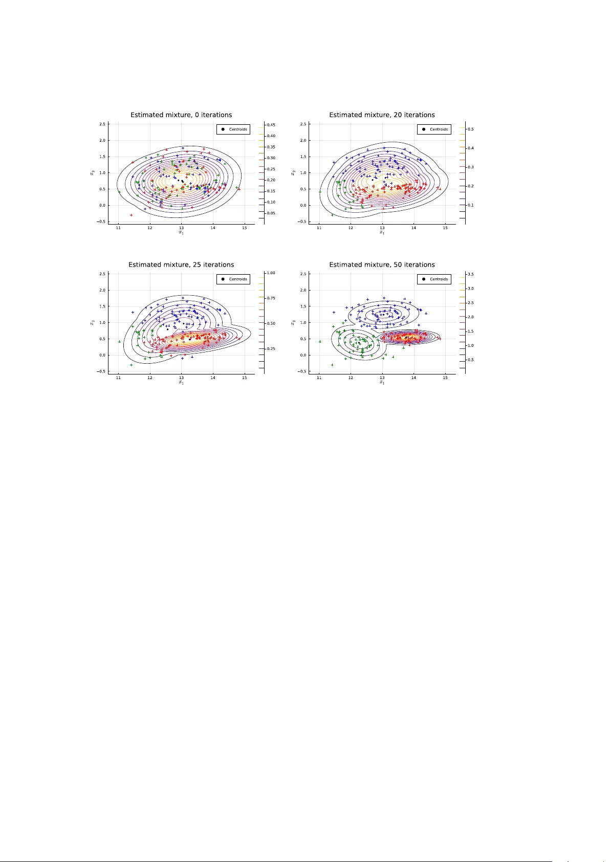
Distributions.jl : Definition and Mo deling of Probabilit y Distributions in the JuliaStats Ecosystem Mathieu Besançon Zuse Institute Berlin Theo dore P apamark ou The Univ ersity of Manc hester Da vid Anthoff Univ ersity of California at Berk eley Alex Arslan Beacon Biosignals, Inc. Simon Byrne California Institute of T ec hnology Dah ua Lin Chinese Univ ersity of Hong K ong John P earson Duk e Universit y Medical Cen ter Abstract Random v ariables and their distributions are a cen tral part in many areas of statistical metho ds. The Distributions.jl pac kage pro vides Julia users and developers to ols for work- ing with probabilit y distributions, lev eraging Julia features for their in tuitive and flexible manipulation, while remaining highly efficient through zero-cost abstractions. K eywor ds : Julia , distributions, mo deling, interface, mixture, KDE, sampling, probabilistic programming, inference. 1. In tro duction The Distributions.jl pac kage ( JuliaStats 2019 ) defines interfaces for represen ting probabilit y distributions and other mathematical objects describing the generation of random samples. It is part of the JuliaStats op en-source organization hosting pac kages for core mathemati- cal and statistical functions ( StatsF uns.jl , PDMats.jl ), mo del fitting ( GLM.jl for generalized linear mo dels, Hyp othesisT ests.jl , MixedMo dels.jl , KernelDensity .jl , Surviv al.jl ) and utilities ( Distances.jl , Rmath.jl ). Distributions.jl defines generic and sp ecific b ehavior required for distributions and other “sample-able” objects. The package implemen ts a large n umber of distributions to b e di- rectly usable for probabilistic mo deling, estimation and simulation problems. It lev erages idiomatic features of Julia including multiple dispatc h and the type system, b oth presented in more detail in Bezanson, Edelman, Karpinski, and Shah ( 2017 ) and Bezanson et al. ( 2018 ). In man y applications, including but not limited to ph ysical sim ulation, mathematical opti- mization or data analysis, computer programs need to generate random num b ers from sample spaces or more sp ecifically from a probabilit y distribution or to infer a probability distribution giv en prior knowledge and observ ed samples. Distributions.jl unifies these use cases under one set of mo deling to ols. 2 Distributions.jl : Probabilit y Distributions in the JuliaStats Ecosystem A core idea of the package is to build an equiv alence b etw een mathematical ob jects and corresp onding Julia t yp es. A probability distribution is therefore represen ted by a type with a given b eha vior provided through the implementation of a set of metho ds. This equiv alence mak es the syntax of programs fit the semantics of the mathematical ob jects. Related soft ware In the scipy.stats 1 mo dule of the SciPy project ( Virtanen et al. 2020 ), distributions are created and manipulated as ob jects in the object-oriented programming sense. Metho ds are defined for a distribution class, then sp ecialized for contin uous and discrete distribution classes inheriting from the generic distribution, from which inherit classes representing actual distribution families. Represen tations of probabilit y distributions ha v e also b een implemen ted in statically-typed functional programming languages, in Hask ell in the Probabilistic F unctional Programming pac kage ( Erwig and Kollmansberger 2006 ), and in OCaml ( Kiselyo v and Shan 2009 ), supp ort- ing only discrete distributions as an asso ciation b etw een collection elemen ts and probabilities. The w ork in Ścibior, Ghahramani, and Gordon ( 2015 ) presents a generic monad-based repre- sen tation of probability distributions allowing for b oth contin uous and discrete distributions. The stats pac kage, whic h is distributed as part of the R language, includes functions related to probabilit y distributions which use a prefix naming conv en tion: r dist for random sampling, d dist for computing the probabilit y densit y , p dist for computing the cumulativ e distribution function, and q dist for computing the quantiles. The distr pac kage ( R uckdesc hel, K ohl, Stabla, and Camphausen 2006 ) also allo ws R users to define their own distribution as a class of the S4 ob ject-oriented system, with four functions r, d, p, q stored by the ob ject. Only one of the four functions has to b e pro vided b y the user when creating a distribution ob ject, the other functions are computed in a suitable wa y . This approac h increases flexibilit y but implies a run time cost dep ending on whic h function has b een pro vided to define a given distribution ob ject. F or instance, when only the random generation function is provided, the RtoDPQ function empirically constructs an estimation for the others, which requires drawing samples instead of directly ev aluating an analytical density . In C++ , the b o ost library ( Bo ost Dev elop ers 2018 ), the maths comp onent includes common distributions and computations up on them. As in Distributions.jl , probabilit y distributions are represen ted by t yp es (classes), as opp osed to functions. The underlying numeric t yp es are rendered generic by the use of templates. The parameters of eac h distribution are accessed through exposed metho ds, while common op erations are defined as non-mem b er functions, th us sharing a similar syn tax with single dispatch. 2 Design and implemen tation prop osals for a m ultiple dispatc h mec hanism in C++ hav e b een inv estigated in Pirk elbauer, Solo dkyy , and Stroustrup ( 2010 ) and describ ed as a library in Le Go c and Donzé ( 2015 ), which would allow for more sophisticated dispatc h rules in the Bo ost distribution interface. This pap er is organized as follo ws. Section 2 presen ts the main t yp es defined in the package and their hierarch y . In Section 3 , the Sampleable t yp e and the asso ciated sampling interface are presen ted. Section 4 presen ts the distribution interface, whic h is the central part of the pac kage. Section 5 presents the av ailable to ols for fitting and estimation of distributions 1 https://docs.scipy.org/doc/scipy/reference/stats.html 2 https://www.boost.org/doc/libs/1_69_0/libs/math/doc/html/math_toolkit/stat_tut/overview/ generic.html Mathieu Besançon, Da vid Anthoff, Alex Arslan, Simon Byrne, Dahua Lin, Theo dore P apamarkou, John Pearson 3 from data using parametric and non-parametric tec hniques. Section 6 presents mo deling to ols and algorithms for mixtures of distributions. Section 7 highligh ts t w o applications of Distributions.jl in related pac kages for k ernel densit y estimation and the implemen tation of Probabilistic Programming Languages in pure Julia . Section 8 concludes on the w ork presen ted and on futu re dev elopment of the ecosystem for probability distributions in Julia . 2. T yp e hierarc h y The Julia language allows the definition of new t yp es and their use for specifying function argumen ts using the multiple dispatch mec hanism ( Zappa Nardelli, Bely ako v a, Pelenitsyn, Ch ung, Bezanson, and Vitek 2018 ). Most common probabilit y distributions can b e broadly classified along tw o facets: • the dimensionalit y of the v alues (e.g., univ ariate, multiv ariate, matrix v ariate) • whether it has discr ete or c ontinuous supp ort, corresp onding to a densit y with resp ect to a coun ting measure or a Leb esgue measure In the Julia t yp e system seman tics, these prop erties can b e captured b y adding t yp e pa- rameters c haracterizing the random v ariable to the distribution t yp e whic h represen ts it. P arametric t yping mak es these pieces of information on the sample space av ailable to the Julia compiler, allo wing dispatc h to b e performed at compile-time, making the op eration a zero-cost abstraction. Distribution is an abstract t yp e that tak es t wo parameters: a VariateForm t yp e whic h describ es the dimensionality , and ValueSupport type whic h describes the discreteness or con tinuit y of the supp ort. These “prop erty types” ha ve singleton subtypes which en umerate these prop erties: julia> abstract type VariateForm end julia> struct Univariate <: VariateForm end julia> struct Multivariate <: VariateForm end julia> struct MatrixVariate <: VariateForm end julia> abstract type ValueSupport end julia> struct Discrete <: ValueSupport end julia> struct Continuous <: ValueSupport end V arious t yp e aliases are then defined for user con v enience: julia> DiscreteUnivariateDistribution = Distribution{Univariate, Discrete} julia> ContinuousUnivariateDistribution = Distribution{Univariate, Continuous} julia> DiscreteMultivariateDistribution = Distribution{Multivariate, Discrete} julia> ContinuousMultivariateDistribution = Distribution{Multivariate, Continuous} The Julia <: op erator in the definition of a new t yp e sp ecifies the direct sup ertype. Sp ecific distribution families are then implemented as sub-types of Distribution : t ypically these are defined as comp osite t yp es (" struct ") with fields capturing the parameters of the distribution. F urther information on the t yp e system can be found in Appendix B . F or example, the univ ariate uniform distribution on ( a, b ) is defined as: julia> struct Uniform{T<:Real} <: ContinuousUnivariateDistribution 4 Distributions.jl : Probabilit y Distributions in the JuliaStats Ecosystem a::T b::T end Note in this case the Uniform distribution is itself a parametric t yp e, this allo ws it to make use of different numeric types. By default these are Float64 , but they can also b e Float32 , BigFloat , Rational , the Dual type from F orwardDiff.jl in order to support features like automatic differentiation ( Rev els, Lubin, and Papamark ou 2016 ), or user defined num b er t yp es. Probabilities are assigned to subsets in a sample space, probabilistic t yp es are qualified based on this sample space from a VariateForm corresp onding to ranks of the samples (scalar, v ector, matrix, tensor) and a ValueSupport corresp onding to the set from which eac h scalar elemen t is restricted. Other t yp es of sample spaces can b e defined for different use cases by implemen ting new sub-t yp es. W e provide t wo examples b elow, one for ValueSupport and one for VariateForm . There are different p ossibilities to represen t sto c hastic pro cesses using the to ols from Distri- butions.jl . One p ossibilit y is to define them as a new ValueSupport type. julia> using Distributions julia> abstract type StochasticProcess <: ValueSupport end julia> struct ContinuousStochasticProcess <: StochasticProcess end julia> abstract type ContinuousStochasticSampler{F<:VariateForm} <: Sampleable{F,ContinuousStochasticProcess} end More complete examples of represen tations of sto chastic pro cesses can b e found in Bridge.jl ( Sc hauer 2018 ). Distributions.jl can also b e extended to supp ort tensor-v ariate random v ari- ables in a similar fashion: julia> using Distributions julia> struct TensorVariate <: VariateForm end julia> abstract type TensorSampleable{S<:ValueSupport} <: Sampleable{TensorVariate,S} end This allo ws other developers to define their o wn mo d els on top of Distributions.jl without requiring the mo dification of the pac kage, while end-users b enefit from the same in terface and con ven tions, regardless of whether one t yp e was defined in Distributions.jl or in an external pac kage. The types describing a probabilistic sampling pro cess then dep end on t w o t yp e parameters inheriting from VariateForm and ValueSupport . The most generic form of suc h a construct is represented b y the Sampleable type, defining something from whic h random samples can b e dra wn: julia> abstract type Sampleable{F<:VariateForm,S<:ValueSupport} end A Distribution is a sub-type of Sampleable , carrying the same t yp e parameter capturing the sample space: julia> abstract type Distribution{F<:VariateForm,S<:ValueSupport} <: Sampleable{F,S} end Mathieu Besançon, Da vid Anthoff, Alex Arslan, Simon Byrne, Dahua Lin, Theo dore P apamarkou, John Pearson 5 A Distribution is more sp ecific than a Sampleable , it describ es the probability law map- ping elements of a σ -algebra (subsets of the sample space) to corresponding probabilities of o ccurrence and is asso ciated with corresp onding probability distribution functions (CDF, PDF). As such, it extends the required interface as detailed in Section 4 . In Distributions.jl , distribution families are represen ted as types and particular distributions as instances of these t yp es. One adv antage of this structure is the ease of defining a new distribution family by creating a sub-t yp e of Distribution resp ecting the in terface. The b ehavior of distributions can also b e extended b y defining new functions ov er all sub-types of Distribution and using the in terface. 3. Sampling in terface Some programs require the generation of random v alues in a certain fashion without requiring the analytical closed-form probability distribution. The Sampleable type and interface serve these use cases. A random quantit y drawn from a sample space with given probability distribution requires a w ay to sample v alues. Suc h construct from which v alues can b e sampled is programmatically defined as an abstract type Sampleable parameterized by F and S . The first type parameter F classifies sampling ob jects and distribution b y their dimension, univ ariate distributions asso ciated with scalar random v ariables, multiv ariate distributions asso ciated with vec tor random v ariables and matrix-v ariate distributions asso ciated with random matrices. The second type parameter S sp ecifies the supp ort, discrete or con tinuous. New v alue supp ort and v ariate form types can also b e defined, subt yp ed from ValueSupport or VariateForm . F urthermore, probability distributions are mathematical functions to consider as immutable. A Sampleable on the other hand can b e a m utable ob ject as shown b elow. Example 3.1. Consider the following implemen tation of a discrete N-state Mark o v chain as a Sampleable . julia> using Distributions julia> mutable struct MarkovChain <: Sampleable{Univariate,Discrete} s::Int m::Matrix{Float64} end A type implementation can only b e a subt yp e of an abstract type as Sampleable . With the structure defined, we can implemen t the required metho d for a Sampleable , namely rand whic h is defined in Base Julia. julia> import Base: rand julia> import Random julia> function rand(rng, mc::MarkovChain) r = rand(rng) v = cumsum(mc.m[mc.s,:]) idx = findfirst(x -> x >= r, v) mc.s = idx return idx end julia> rand(mc::MarkovChain) = rand(Random.GLOBAL_RNG, mc) 6 Distributions.jl : Probabilit y Distributions in the JuliaStats Ecosystem rng is a random num b er generator (RNG) ob ject, passing it as an argumen t makes the rand implemen tation predictable. If repro ducibility is not imp ortant to the use case, rand can b e called as rand(mc) as implemen ted in the second metho d, using the global random num b er generator Random.GLOBAL_RNG . Note that the Mark ov c h ain implemen tation could hav e b een defined in an immutable wa y . This implementations how ever highlights one possible definition of a Sampleable different from a probabilit y distribution. This flexibilit y of implementation comes with a homogeneous in terface, any item from which random samples can b e generated is called in the same fashion. F rom the user p ersp ectiv e, where a sampler is defined has no impact on its use thanks to Julia multiple dispatch mechanism: the correct metho d (function implementation) is called dep ending on the input t yp e. The rand function is the only required element for defining the sampling with a particular pro cess. Differen t metho ds are defined for this function, sp ecifying the pseudo-random n um- b er generator (PRNG) to b e used. The default RNG uses the Mersenne-T wister algorithm ( Matsumoto and Nishimura 1998 ). The sampling state is kept in a global v ariable used by default when no RNG is provided. New random num b er generators can b e defined b y users, sub-t yp ed from the Random.AbstractRNG t yp e. 4. Distribution in terface and t yp es The core of the package are probabilit y distributions, defined as an abstract t yp e as pre- sen ted in 2 . An y distribution m ust implement the rand metho d, which means random v alues follo wing the distribution can b e generated. The t wo other essen tial metho ds to implement are pdf giving the probability densit y function at one point for con tinuous distributions or the probability mass function at one point for discrete distributions and cdf ev aluat- ing the Cumulated Densit y F unction at one p oint. The quantile method from the stan- dard library Statistics mo dule can be implemented for a Distribution type, with the form quantile(d::Distribution,p::Number) and returning the v alue corresp onding to the cor- resp onding cumulativ e probabilit y p . Give n that the method rand() without any argumen t follo ws a uniform pseudo-random num b er in the in terv al [0 , 1] , a default fall-bac k method for random num b er generation can b e defined b y in v erse transform sampling for a univ ariate distribution as: julia> rand(d::UnivariateDistribution) = quantile(d, rand()) The equiv alen t R functions for the normal distribution can b e matched to the Distributions.jl w ay of expressing them as follows: julia> using Distributions julia> rnorm(n, mu, sig) = rand(Normal(mu, sig), n) julia> dnorm(x, mu, sig) = pdf(Normal(mu, sig), x) julia> pnorm(x, mu, sig) = cdf(Normal(mu, sig), x) julia> qnorm(p, mu, sig) = quantile(Normal(mu, sig), p) The adv antage of using multiple dispatc h is that supp orting a new distribution only requires the package API to grow b y one elemen t whic h is the new distribution type, instead of four new functions. Most common probability distributions are defined by a mathematical form and a set of parameters. All distributions must implemen t the params metho d from the Mathieu Besançon, Da vid Anthoff, Alex Arslan, Simon Byrne, Dahua Lin, Theo dore P apamarkou, John Pearson 7 StatsBase.jl , allowing the f ollo wing example to alwa ys w ork for any given distribution type Dist and d an instance of the distribution: julia> p = params(d) julia> new_dist = Dist(p...) Dep ending on the distribution, sampling a batch of data can b e done in a more efficien t manner than multiple individual samples. Sp ecialized samplers can b e provided for distribu- tions, letting user sample batches of v alues. Sampling from the Kolmogoro v distribution for instance is done b y pulling atomic samples using an alternating series metho d ( Devroy e 1986 , IV.5), while the P oisson distribution lets users use either a coun ting sampler or Ahrens-Dieter sampler ( Ahrens and Dieter 1982 ). W e will not expand explanations on most trivial functions of the distribution interface, suc h as minimum , maximum whic h can b e defined in terms of support . Other v alues are optional to define for distributions, such as mean , median , variance . Not defining these metho ds as mandatory allo ws for instance for the Cauch y-Lorentz distribution to b e defined. 5. Distribution fitting and estimation Giv en a collection of samples and a distribution dep enden t on a vector of parameters, the distribution fitting task consists in finding an estimation of the distribution parameters ˆ θ . 5.1. Maximum lik eliho o d estimation Maxim um Likelihoo d is a common technique for estimating the parameters θ of a distribution giv en observ ations ( Wilks 1938 ; Aldrich 1997 ), with numerous applications in statistics but also in signal pro cessing ( Pham and Garat 1997 ). The Distributions.jl in terface is defined as one fit_mle function with t wo metho ds: Distributions.fit_mle(D, x) Distributions.fit_mle(D, x, w) With D a distribution t yp e to fit, x b eing either a v ector of observ ations if D is univ ariate, a ma- trix of individuals/attributes if D is m ultiv ariate, and w weigh ts for the individual data p oints. The function call returns an instance of D with the parameter adjusted to the observ ations from x . Example 5.1. Fitting a normal distribution b y maximum likelihoo d. julia> using Distributions julia> import Random julia> Random.seed!(33) julia> xs = rand(Normal(50.0, 10.0), 1000) julia> fit_mle(Normal, xs) Distributions.Normal{Float64}( µ =49.781, σ =10.002) A dditional partial information can b e provided with distribution-sp ecific keyw ords. fit_mle(Normal, x) accepts for instance the keyw ord arguments mu and sigma to sp ecify either a fixed mean or standard deviation. 8 Distributions.jl : Probabilit y Distributions in the JuliaStats Ecosystem The maximum likelihoo d estimation (MLE) function is implemen ted for sp ecific distribution t yp es, corresp onding to the fact that there is no default and efficient MLE algorithm for a generic distribution. The implementations present in Distributions.jl only require the com- putation of sufficien t statistics. F or a more adv anced use cases, section D.3 presen ts the maximization of the likelihoo d for a custom distribution ov er a real dataset with a Cartesian pro duct of univ ariate distributions. The b ehavior can b e extended to a new distribution t yp e D b y implementing fit_mle for it: julia> using Distributions julia> struct D <: ContinuousUnivariateDistribution end julia> function Distributions.fit_mle(::Type{D}, xs::AbstractVector) # implementation end 5.2. Non-parametric estimation Some distribution estimation tasks hav e to b e carried out without the kno wledge of the dis- tribution form or family for v arious reasons. Non-parametric estimation generally comprises the estimation of the Cum ulative Density F unction and of the Probability Densit y F unction. StatsBase.jl provides the ecdf function, a higher order function returning the empirical CDF at any new p oint. Since the empirical CDF is built as a weigh ted sum of Heaviside functions, it is discon tinuous. StatsBase.jl also pro vides a generic fit function, used to build density histograms. Histogram is a t yp e storing the bins and heigh ts, other functions from Base Julia are defined on Histogram for con venience. fit for histogram is defined with the following signature: StatsBase.fit(Histogram, data[, weight][, edges]; closed=:right, nbins) 6. Mo deling mixtures of distributions Mixture mo dels are used for mo deling p opulations which consists of multiple sub-p opulations; mixture mo dels are often applied to clustering or noise separation tasks. A mixture distribution consists of sev eral c omp onent distributions , eac h of which has a relativ e c omp onent weight or c omp onent prior pr ob ability . F or a mixture of n comp onen ts, then the densities can b e written as a w eigh ted sum: f mix ( x ; π , θ ) = n X i =1 π i f ( x, θ i ) where the parameters are the comp onent weigh ts π = ( π 1 , . . . , π n ) , taking v alues on the unit simplex, and eac h θ i parameterizes the i th comp onen t distribution. Sampling from a mixture model consists of first selecting the comp onen t according to the relativ e w eight, then sampling from the corresp onding comp onen t distribution. Therefore a mixture mo del can also b e interpreted as a hierarc hical mo del. Mixtures are defined as an abstract sub-type of Distribution , parameterized by the same t yp e information on the v ariate form and v alue supp ort: Mathieu Besançon, Da vid Anthoff, Alex Arslan, Simon Byrne, Dahua Lin, Theo dore P apamarkou, John Pearson 9 julia> abstract type AbstractMixtureModel{VF<:VariateForm,VS<:ValueSupport} <: Distribution{VF, VS} end An y AbstractMixtureModel is therefore a Distribution and therefore implements sp ecial- ized the mandatory metho ds insupport , mean , var , etc. Mixture mo dels also need to imple- men t the following b ehavior: • ncomponents(d::AbstractMixtureModel) : returns the n umber of comp onents in the mixture • component(d::AbstractMixtureModel, k) : returns the k-th comp onen t • probs(d) : returns the vector of prior probabilities ov er comp onents A concrete generic implemen tation is then defined as: julia> struct MixtureModel{VF<:VariateForm,VS<:ValueSupport,Component<:Distribution} <: AbstractMixtureModel{VF,VS} components::Vector{Component} prior::Categorical end Once constructed, it can b e manipulated as an y distribution with the differen t metho ds of the in terface. Example 6.1. Figure 1 shows the plot resulting from the follo wing construction of a uni- v ariate Gaussian mixture mo del. julia> using Distributions julia> import Plots julia> gmm = MixtureModel( Normal.([-1.0, 0.0, 3.0], [0.3, 0.5, 1.0]), [0.25, 0.25, 0.5], ) julia> xs = -2.0:0.01:6.0 julia> Plots.plot(xs, pdf.(gmm, xs), legend=nothing) julia> Plots.ylabel!("\$f_X(x)\$") julia> Plots.xlabel!("\$x\$") julia> Plots.title!("Gaussian mixture PDF") The MixtureModel constructor is taking as argument a vector of Normal distributions, defined here from a v ector of mean v alues and a vector of standard deviation v alues. Mixture mo dels remain an activ e area of research and of dev elopment within Distributions.jl , estimation metho ds, and impro v ed multiv ariate and matrix-v ariate supp ort are plann ed for future releases. A more adv anced example of estimation of a Gaussian mixture b y a generic EM algorithm is presen ted in section D.4 . 7. Applications of Distributions.jl 10 Distributions.jl : Probabilit y Distributions in the JuliaStats Ecosystem Figure 1: Example PDF of a univ ariate Gaussian mixture Distributions.jl has become a foundation for statistical programming in Julia , notably used for economic mo deling ( F ederal Reserv e Bank Of New Y ork 2019 ; Lyon, Sargent, and Stach urski 2017 ), Marko v chain Monte Carlo simulations ( Smith 2018 ) or randomized black-box opti- mization F eldt ( 2017 ) 3 . W e presen t b elo w tw o applications of the package for non -parametric con tinuous density estimation and probabilistic programming. 7.1. Kernel density estimation Probabilit y densit y functions can b e estimated in a non-parametric fashion using kernel den- sit y estimation (KDE, Rosenblatt 1956 ; Parzen 1962 ). This is supp orted through the Ker- nelDensit y .jl pac kage, defining the kde function to infer an estimate density from data. Both univ ariate and biv ariate density estimates are supp orted. Most of the algorithms and param- eter selection heuristics developed in KernelDensity .jl are based on Silverman ( 2018 ). Ker- nelDensit y .jl supp orts m ultiple distributions as base kernels, and can b e extended to other families. The default kernel used is Gaussian. Example 7.1. W e highlight the estimation of a kernel density on data generated from the mixture of a log-normal and uniform distributions. julia> import Random, Plots, KernelDensity julia> using Distributions julia> function generate_point(rng = Random.GLOBAL_RNG) thres = rand(rng) if thres >= 0.5 rand(rng, LogNormal()) else rand(rng, Uniform(2.0, 3.0)) end end julia> mt = Random.MersenneTwister(42) julia> xs = [generate_point(mt) for _ in 1:5000] 3 Other packages depending on Distributions.jl can b e found on the Julia General registry: https://github. com/JuliaRegistries/General Mathieu Besançon, Da vid Anthoff, Alex Arslan, Simon Byrne, Dahua Lin, Theo dore P apamarkou, John Pearson 11 Figure 2: A djusted KDE with v arious bandwidths julia> bandwidths = [0.05, 0.1, 0.5] julia> densities = [KernelDensity.kde(xs, bandwidth = bw) for bw in bandwidths] julia> p = Plots.plot() julia> for (b,d) in zip(bandwidths, densities) Plots.plot!(p, d.x, d.density, labels = "bw = $b") end julia> Plots.xlims!(p, 0.0, 8.0) julia> Plots.title!("KDE with Gaussian Kernel") The bandwidth bw = 0 . 1 seems not to o verfit isolated data p oin ts without smo othing out imp ortan t comp onents. All examples pro vided use the Plots.jl 4 pac kage to plot results, whic h can b e used with v arious plotting engines as bac k-end. W e can compare the kernel densit y estimate to the real PDF as done in the following script and illustrated Figure 3 . julia> xvals = 0.01:0.01:8.0 julia> yvals = map(xvals) do x comp1 = pdf(LogNormal(), x) comp2 = pdf(Uniform(2.0, 3.0), x) 0.5 * comp1 + 0.5 * comp2 end julia> p = Plots.plot(xvals, yvals, labels = "Real distribution") julia> kde = KernelDensity.kde(xs, bandwidth = 0.1) julia> Plots.plot!(p, kde.x, kde.density, labels = "KDE") julia> Plots.plot!(p, xvals, yvals, labels = "Real distribution") julia> Plots.xlims!(p, 0.0, 8.0) The kernel density estimation tec hnique relies on a base distribution (the k ernel) whic h is con voluted against the data. The pac kage uses directly the in terface presented in section 4 to accept a Distribution as second parameter. The follo wing script computes the kernel density estimates with a Gaussian and triangular distributions. The result is illustrated Figure 4 . julia> mt = Random.MersenneTwister(42) 4 h ttp://do cs.juliaplots.org 12 Distributions.jl : Probabilit y Distributions in the JuliaStats Ecosystem Figure 3: Comparison of the exp erimen tal and real PDF Figure 4: Comparison of different kernels defined as Distribution ob jects julia> ( µ , σ ) = (5.0, 1.0) julia> xs = [rand(mt, Normal( µ , σ )) for _ in 1:50] julia> ndist = Normal(0.0, 0.3) julia> gkernel = kde(xs, ndist) julia> tdist = TriangularDist(-0.5, 0.5) julia> tkernel = KernelDensity.kde(xs, tdist) julia> p = Plots.plot(tkernel.x, tkernel.density, labels = "Triangular kernel") julia> Plots.plot!(p, gkernel.x, gkernel.density, labels = "Gaussian kernel", legend = :left) julia> Plots.title!(p, "Comparison of Gaussian and triangular kernels") The density estimator is computed via the F ourier transform: any distribution with a defined c haracteristic function (via the cf function from Distributions.jl ) can b e used as a k ernel. The abilit y to manipulate distributions as t yp es and ob jects allo ws end-users and pac kage dev elop ers to compose on top of defined distributions and to define their own to use for k ernel densit y estimations without an y additional run time cost. The kernel estimation of a bi-v ariate Mathieu Besançon, Da vid Anthoff, Alex Arslan, Simon Byrne, Dahua Lin, Theo dore P apamarkou, John Pearson 13 densit y is shown in D.2 . 7.2. Probabilistic programming languages Probabilistic programs are computer programs with the added capability of dra wing the v alue of a v ariable from a probability distribution and conditioning v ariable v alues on observ ations ( Gordon, Henzinger, Nori, and Rajamani 2014 ). They allow for the sp ecification of complex relations b etw een random v ariables using a set of constructs that go b eyond t ypical graphical mo dels to include flo w con trol (e.g., lo ops, conditions), recursion, user-defined t yp es and other algorithmic building blo c ks, differing from explicit graph construction by users, as done for instance in Smith ( 2018 ). Probabilistic programming languages (PPL) are programming language or libraries enabling developers to write such a probabilistic program. That is, they are a t yp e of domain-sp ecific language (DSL, F owler 2010 ). W e refer the interested reader to V an de Meen t, P aige, Y ang, and W o o d ( 2018 ) for an ov erview of PPL design and use, to Ścibior et al. ( 2017 ) for the analysis of Bay esian inference algorithms as transformations of in termediate representations, and to Vákár, Kammar, and Staton ( 2019 ) for representation of recursiv e types in PPLs. They often fall in tw o categories. In the first type, the PPL is its o wn indep endent language, including syntax and parsing, though it may rely on another “host” language for its execution engine. F or example, Stan ( Carp en ter et al. 2017 ), uses its o wn .stan mo del sp ecification format, though the parser and inference engine are written in C++ . This type of approach b enefits from defining its o wn syn tax, thus designing it to lo ok similar to the wa y equiv alen t statistical mo dels are written. The mo del is also v erified for syn tactic correctness at compile-time. 5 In the second type of PPL, the language is embedded within and makes use of the syn tax of the host language, leveraging that language’s native constructs. F or example, PyMC ( P atil, Huard, and F onnesb eck 2010 ; K o ch urov, Carroll, Wiecki, and Lao 2019 ), Pyro ( Bingham et al. 2019 ), and Edward ( T ran, Kucukelbir, Dieng, Rudolph, Liang, and Blei 2016 ) all use Python as the host language, lev eraging Theano , T orch , and T ensorFlow , respectively , to p erform man y of the underlying inference computations. Here, the key adv antage is that these PPLs gain access to the ecosystem of the host language (data structures, libraries, to oling). User do cumen tation and dev elopment efforts can also fo cus on the key aspects of a PPL instead of the full stac k. 6 Ho wev er, b oth approaches to PPLs suffer from drawbac ks. In the first type of PPLs, users m ust add new elements to their to olchains for the developmen t and inference of statistical mo dels. That is, they are likely to use a general-purp ose programming language for other tasks, then switch to the PPL en vironment for the sampling and inference task, and then read the result back in to the general-purp ose programming language. One solution to this problem is to develop APIs in general purp ose languages, but full inter-operability b etw een t wo en vironments is non-trivial. Dev elop ers must then build a whole ecosystem around the PPL, including data structures, input/output, and text editor supp ort, which costs time that migh t otherwise go tow ard improving the inference algorithms and optimization pro cedures. While the second type of PPL may not require the developmen t of a separate, parallel set of to ols, it often runs into “imp edance mismatc hes” of its o wn. In many cases, the host language has not been designed for a re-use of its constructs for probabilistic programming, resulting 5 An example mo del combining Stan with R can be found at Gelman ( 2019 ). 6 The same golf putting data were used using PyMC as PPL in PyMC ( 2019 ). 14 Distributions.jl : Probabilit y Distributions in the JuliaStats Ecosystem in syn tax that aligns p o orly with users’ mathematical in tuitions. Moreo ver, duplication may still o ccur at the level of classes or libraries, as, for example, Pyro and Edward dep end on T orc h and T ensorFlo w, which replicate m uch of the linear algebra functionality of NumPy for their o wn array constructs. By contrast, the design of Distributions.jl has enabled the dev elopment of embedded prob- abilistic programming languages such as T uring.jl ( Ge, Xu, and Ghahramani 2018 ), SOSS.jl ( Sc herrer 2019 ), Omega.jl ( T av ares 2018 ) or Poirot.jl ( Innes 2019 ) with comparatively less o verhead or friction with the host language. These PPLs are able to make use of three el- emen ts unique to the Julia ecosystem to c hallenge the dic hotomy b etw een embedded and stand-alone PPLs. First, they mak e use of Julia ’s rich type system and multiple dispatc h, whic h more easily supp ort mo deling mathematical constructs as types. Second, they all utilize Distributions.jl ’s types and hierarch y for the sampling of random v alues and representation of their distributions. Finally , they use manipulations and transformations of the user Julia co de to create new syn tax that matc hes domain-sp ecific requiremen ts. These transformations are either p erformed through macros (for Soss.jl and T uring.jl ) or mo d- ifications of the compilation phases through compiler ov erdubbing ( Omega.jl and Poirot.jl use Cassette.jl and IR T o ols.jl resp ectiv ely to mo dify the user co de or its in termediate representa- tions). As in the Lisp tradition, Julia ’s macros are written and manipulable in Julia itself and rewrite co de during the lo w ering phase ( Bezanson et al. 2018 ). Macros allow PPL design- ers to k eep programs close to s tandard Julia while introducing package-specific syntax that more closely mimics statistical conv en tions, all without compromising on p erformance. F or instance, a simple mo del definition from the T uring.jl do cumentation illustrates a mo del that is b oth readable as Julia co de while staying close to statistical conv en tions: julia> @model coinflip(y) = begin p ~ Beta(1, 1) N = length(y) for n in 1:N y[n] ~ Bernoulli(p) end end With these syn tax manipulation capabilities, along with compiled language p erformance, the com bination of Julia with Distributions.jl pro vides an excellen t foundation for further researc h and dev elopment of PPLs. 7 8. Conclusion and future w ork W e presen ted some of the types, structures and to ols for mo deling and computing on prob- abilit y distributions in the JuliaStats ecosystem. The JuliaStats packages lev erage some key constructs of Julia suc h as definition of new comp osite t yp es, abstract parametric t yp es and sub-t yping, along with m ultiple dispatc h. This allows users to express computations inv olving random num b er generation and the manipulation of probabilit y distributions. A clear inter- face allows package developers to build new distributions from their mathematical definition. New algorithms can b e dev elop ed, using the Distribution in terface and as suc h extending the 7 The golf putting mo del was p orted to T uring.jl in Duncan ( 2020 ). Mathieu Besançon, Da vid Anthoff, Alex Arslan, Simon Byrne, Dahua Lin, Theo dore P apamarkou, John Pearson 15 new features to all sub-t yp es. These tw o features of Julia , namely extension of b ehavior to new types and definition of behavior ov er existing type hierarc hy , allow different features built around the Distribution type to in ter-op erate seamlessly without hard coupling nor additional w ork from the package dev elop ers or end-users. F uture w ork on the package will include the implemen tation of maximum lik eliho o d estimation for other distributions, including mixtures and matrix-v ariate distributions. A c kno wledgmen ts The authors thank and ackno wledge the w ork of all contributors and maintainers of packages of the JuliaStats ecosystem and esp ecially Dav e Kleinsc hmidt for his v aluable feedback on early v ersions of this article, Andreas Noac k for the ov erall sup ervision of the pac kage, including the in tegration of n umerous pull requests from external con tributors, Moritz Sc hauer for discussions on the represen tability of mathematical objects in the Julia type system and Zenna T a v ares for the critical review of early drafts. Researc h sp onsored by the Lab oratory Directed Researc h and Developmen t Program of Oak Ridge National Laboratory , managed by UT-Battelle, LLC, for the US Departmen t of Energy under con tract DE-A C05-00OR22725. This researc h used resources of the Compute and Data En vironment for Science (CADES) at the Oak Ridge National Lab oratory , whic h is supp orted by the Office of Science of the U.S. Department of Energy under Contract No. DE- A C05-00OR22725. This applies specifically to funding pro vided by the Oak Ridge National Lab oratory to Theo dore Papamark ou. References A eb erhard S, Co omans D, De V el O (1994). “Comparativ e Analysis of Statistical Pattern Recognition Metho ds in High Dimensional Settings. ” Pattern R e c o gnition , 27 (8), 1065– 1077. doi:10.1016/0031- 3203(94)90145- 7 . Ahrens JH, Dieter U (1982). “Computer Generation of P oisson Deviates from Modified Normal Distributions. ” A CM T r ansactions on Mathematic al Softwar e , 8 (2), 163–179. doi: 10.1145/355993.355997 . Aldric h J (1997). “R.A. Fisher and the Making of Maximum Likelihoo d 1912–1922. ” Statistic al Scienc e , 12 (3), 162–176. doi:10.1214/ss/1030037906 . Bezanson J, Chen J, Chung B, Karpinski S, Shah VB, Vitek J, Zoubritzky L (2018). “ Julia : Dynamism and Performance Reconciled by Design. ” Pr o c e e dings of the A CM on Pr o gr am- ming L anguages , 2 (OOPSLA), 120. doi:10.1145/3276490 . Bezanson J, Edelman A, Karpinski S, Shah V (2017). “ Julia : A F resh Approac h to Numerical Computing. ” SIAM R eview , 59 (1), 65–98. doi:10.1137/141000671 . Bingham E, Chen JP , Jank owiak M, Ob ermeyer F, Pradhan N, Karaletsos T, Singh R, Szerlip P , Horsfall P , Go o dman ND (2019). “ Pyro : Deep Univ ersal Probabilistic Programming. ” The Journal of Machine L e arning R ese ar ch , 20 (1), 973–978. 16 Distributions.jl : Probabilit y Distributions in the JuliaStats Ecosystem Bo ost Dev elop ers (2018). “ Bo ost C++ Libraries. ” URL https://www.boost.org/ . Carp en ter B, Gelman A, Hoffman MD, Lee D, Go o drich B, Betancourt M, Brubaker M, Guo J, Li P , Riddell A (2017). “ Stan : A Probabilistic Programming Language. ” Journal of Statistic al Softwar e , 76 (1), 1–32. doi:10.18637/jss.v076.i01 . Devro ye L (1986). Non-Uniform R andom V ariate Gener ation . Springer-V erlag, New Y ork. Duncan J (2020). “Mo del building of golf putting with T uring.jl . ” URL https://web.archive.org/web/20210611145623/https://jduncstats.com/posts/ 2019- 11- 02- golf- turing/ . Erwig M, K ollmansb erger S (2006). “F unctional Pearls: Probabilistic F unctional Program- ming in Hask ell . ” Journal of F unctional Pr o gr amming , 16 (1), 21–34. doi:10.1017/ s0956796805005721 . F ederal Reserve Bank Of New Y ork (2019). “ DSGE.jl : Solv e and Estimate Dynamic Sto chastic General Equilibrium Mo dels (Including the New Y ork F ed DSGE). ” URL https://github. com/FRBNY- DSGE/DSGE.jl . F eldt R (2017). “ Blac kBoxOptim.jl . ” URL https://github.com/robertfeldt/ BlackBoxOptim.jl . F o wler M (2010). Domain-Sp e cific L anguages . P earson Education. Ge H, Xu K, Ghahramani Z (2018). “ T uring : Comp osable Inference for Probabilistic Pro- gramming. ” In Pr o c e e dings of the Twenty-First International Confer enc e on A rtificial Intel- ligenc e and Statistics , pp. 1682–1690. URL http://proceedings.mlr.press/v84/ge18b. html . Gelman A (2019). “Mo del Building and Expansion for Golf Putting (accessed June 2021). ” URL https://mc- stan.org/users/documentation/case- studies/golf.html . Gordon AD, Henzinger T A, Nori A V, Ra jamani SK (2014). “Probabilistic Programming. ” In Pr o c e e dings of the on F utur e of Softwar e Engine ering , pp. 167–181. ACM. Innes M (2019). “ Poirot.jl . ” V ersion 0.1, URL https://github.com/MikeInnes/Poirot.jl . JuliaStats (2019). “ Distributions.jl . ” doi:10.5281/zenodo.2647458 . Kisely ov O, Shan CC (2009). “Embedded Probabilistic Programming. ” In WM T aha (ed.), Domain-Sp e cific L anguages , pp. 360–384. Springer-V erlag, Berlin. K o c huro v M, Carroll C, Wiecki T, Lao J (2019). “ PyMC4 : Exploiting Coroutines for Im- plemen ting a Probabilistic Programming F ramew ork. ” URL https://openreview.net/ forum?id=rkgzj5Za8H . Le Go c Y, Donzé A (2015). “ EVL : A F ramew ork for Multi-Metho ds in C++ . ” Scienc e of Computer Pr o gr amming , 98 , 531–550. ISSN 0167-6423. doi:10.1016/j.scico.2014.08. 003 . Ly on S, Sargen t TJ, Stac hurski J (2017). “ QuantEcon.jl . ” URL https://github.com/ QuantEcon/QuantEcon.jl . Mathieu Besançon, Da vid Anthoff, Alex Arslan, Simon Byrne, Dahua Lin, Theo dore P apamarkou, John Pearson 17 Matsumoto M, Nishim ura T (1998). “Mersenne T wister: A 623-Dimensionally Equidistributed Uniform Pseudo-Random Number Generator. ” A CM T r ansactions on Mo deling and Com- puter Simulation , 8 (1), 3–30. doi:10.1145/272991.272995 . Mogensen PK, Riseth AN (2018). “ Optim : A Mathematical Optimization P ac kage for Julia . ” Journal of Op en Sour c e Softwar e , 3 (24), 615. doi:10.21105/joss.00615 . Orban D, Siqueira AS (2019). “ JuliaSmo othOptimizers : Infrastructure and Solvers for Con- tin uous Optimization in Julia . ” doi:10.5281/zenodo.2655082 . P arzen E (1962). “On Estimation of a Probability Density F unction and Mo de. ” The A nnals of Mathematic al Statistics , 33 (3), 1065–1076. doi:10.1214/aoms/1177704472 . P atil A, Huard D, F onnesb eck C (2010). “ PyMC : Bay esian Sto c hastic Mo delling in Python . ” Journal of Statistic al Softwar e , 35 (4), 1–81. doi:10.18637/jss.v035.i04 . Pham DT, Garat P (1997). “Blind Separation of Mixture of Independent Sources through a Quasi-Maxim um Likelihoo d Approach. ” IEEE T r ansactions on Signal Pr o c essing , 45 (7), 1712–1725. doi:10.1109/78.599941 . Pirk elbauer P , Solo dkyy Y, Stroustrup B (2010). “Design and Ev aluation of C++ Open Multi- Metho ds. ” Scienc e of Computer Pr o gr amming , 75 (7), 638–667. doi:10.1016/j.scico. 2009.06.002 . Generativ e Programming and Comp onent Engineering (GPCE 2007). PyMC (2019). “Mo del building and expansion for golf putting. ” URL http: //web.archive.org/web/20191210110708/https://nbviewer.jupyter.org/github/ pymc- devs/pymc3/blob/master/docs/source/notebooks/putting_workflow.ipynb . Rev els J, Lubin M, Papamark ou T (2016). “F orw ard-Mo de Automatic Differen tiation in Julia . ” arXiv 1607.07892 , arXiv.org E-Prin t Archiv e. URL . Rosen blatt M (1956). “Remarks on Some Nonparametric Estimates of a Density F unction. ” The A nnals of Mathematic al Statistics , 27 (3), 832–837. doi:10.1214/aoms/1177728190 . R uckdesc hel P , Kohl M, Stabla T, Camphausen F (2006). “ S 4 Classes for Distributions. ” R News , 6 (2), 2–6. Sc hauer M (2018). “ Bridge.jl : a Statistical T o olb o x for Diffusion Pro cesses and Sto c hastic Differen tial Equations. ” doi:10.5281/zenodo.891230 . V ersion 0.9. Sc herrer C (2019). “ Soss.jl : Probabilistic Programming via Source Rewriting. ” V ersion 0.1, URL https://github.com/cscherrer/Soss.jl . Ścibior A, Ghahramani Z, Gordon AD (2015). “Practical Probabilistic Programming with Monads. ” A CM SIGPLAN Notic es , 50 (12), 165–176. doi:10.1145/2887747.2804317 . Ścibior A, Kammar O, Vákár M, Staton S, Y ang H, Cai Y, Ostermann K, Moss SK, Heunen C, Ghahramani Z (2017). “Denotational V alidation of Higher-Order Bay esian Inference. ” Pr o c e e dings of the A CM on Pr o gr amming L anguages , 2 , 60. doi:10.1145/3158148 . Silv erman BW (2018). Density Estimation for Statistics and Data A nalysis . Routledge. 18 Distributions.jl : Probabilit y Distributions in the JuliaStats Ecosystem Smith BJ (2018). “ Mam ba.jl : Marko v Chain Mon te Carlo (MCMC) for Bay esian Analysis in Julia . ” V ersion 0.12, URL https://github.com/brian- j- smith/Mamba.jl . T a v ares Z (2018). “ Omega.jl : Causal, Higher-Order, Probabilistic Programming. ” V ersion 0.1, URL https://github.com/zenna/Omega.jl . T ran D, Kucukelbir A, Dieng AB, R udolph M, Liang D, Blei DM (2016). “ Edward : A Library for Probabilistic Mo deling, Inference, and Criticism. ” arXiv 1610.09787 , arXiv.org E-Print Arc hive. URL . Vákár M, Kammar O, Staton S (2019). “A Domain Theory for Statistical Probabilistic Programming. ” Pr o c e e dings of the A CM on Pr o gr amming L anguages , 3 (POPL), 36. doi: 10.1145/3290349 . V an de Meen t JW, Paige B, Y ang H, W oo d F (2018). “An Introduction to Probabilistic Programming. ” arXiv 1809.10756 , arXiv.org E-Prin t Arc hive. URL abs/1809.10756 . Virtanen P , Gommers R, Oliphan t TE, Hab erland M, Reddy T, Cournap eau D, Burovski E, Peterson P , W ec kesser W, Brigh t J, v an der W alt SJ, Brett M, Wilson J, Millman KJ, Ma yoro v N, Nelson ARJ, Jones E, Kern R, Larson E, Carey CJ, Polat İ, F eng Y, Mo ore EW, V anderPlas J, Laxalde D, Perktold J, Cimrman R, Henriksen I, Quintero EA, Harris CR, Archibald AM, Ribeiro AH, P edregosa F, v an Mulbregt P , SciPy 10 Con tributors (2020). “ SciPy 1.0: F undamental Algorithms for Scientific Computing in Python . ” Natur e Metho ds , 17 , 261–272. doi:10.1038/s41592- 019- 0686- 2 . Wilks SS (1938). “The Large-Sample Distribution of the Likelihoo d Ratio for T esting Comp osite Hyp otheses. ” The A nnals of Mathematic al Statistics , 9 (1), 60–62. doi: 10.1214/aoms/1177732360 . Zappa Nardelli F, Belyak ov a J, Pelenitsyn A, Chung B, Bezanson J, Vitek J (2018). “ Julia Subt yping: A Rational Reconstruction. ” Pr o c e e dings of the A CM on Pr o gr amming L an- guages , 2 (OOPSLA), 113. doi:10.1145/3276483 . Mathieu Besançon, Da vid Anthoff, Alex Arslan, Simon Byrne, Dahua Lin, Theo dore P apamarkou, John Pearson 19 A. Installation of the relev ant pac kages The recommended installation of the relev an t pac kages is done through the Pkg.jl 8 to ol av ail- able within the Julia distribution standard library . The common w ay to interact with the to ol is within the REPL for Julia 1.0 and ab o v e. The closing square brack et "]" starts the pkg mo de, in whic h the REPL sta ys un til a return key is stroke. julia> ] add StatsBase (v1.0) pkg> add Distributions (v1.0) pkg> add KernelDensity This installation and all co de snippets are guaran teed to w ork on Julia 1.0 and later with the semantic versioning commitment. Once installed, a package can b e remov ed with the command rm PackageName or up dated. All package mo difications are guaran teed to resp ect v ersion constrain ts for their direct and transitiv e dep endencies. The packages StatsBase.jl , Distributions.jl , KernelDensit y .jl are all op en-source under the MIT license. B. Julia t yp e system B.1. F unctions and metho ds In Julia , a function “is an ob ject that maps a tuple of argument v alues to a return v alue” . 9 A sp ecial case is an empty tuple as input, as in y = f() , and a function that returns the nothing v alue. A function definition creates a top-lev el identifier with the function name. This can b e passed around as any other v alue, for example to other functions. The function map takes a function and a collection map(f, c) , and applies the function to each elemen t of the collection to return the mapp ed v alues. A function migh t represen t a conceptual computation but different sp ecific implementations migh t exist for this computation. F or instance, the addition of tw o num b ers is a common concept, but ho w it is implemented dep ends on the n umber t yp e. The sp ecific implementation of addition for complex n um b ers is 10 julia> +(z::Complex, w::Complex) = Complex(real(z) + real(w), imag(z) + imag(w)) This sp ecific implementation is a metho d of the + function. Users can define their own implemen tation of existing functions, thus creating a new metho d for this function. Differen t metho ds can b e implemented b y changing the tuple of argumen ts, either with a different n umber of arguments or different types. 11 Example B.1. In the follo wing example, the function f has tw o metho ds. The function called dep ends on the n um b er of argumen ts. 8 https://docs.julialang.org/en/v1/stdlib/Pkg/ 9 Julia do cumen tation - F unctions: https://docs.julialang.org/en/v1/manual/functions 10 Julia source co de, base/complex.jl 11 Julia do cumen tation - Metho ds: https://docs.julialang.org/en/v1/manual/methods 20 Distributions.jl : Probabilit y Distributions in the JuliaStats Ecosystem julia> function f(x) println(x) end julia> function f(x, y) println("x: $x & y: $y") end Example B.2. In the following example, the function g has tw o metho ds. The first one is the most sp ecific metho d and will b e called for any type of the argument x that is a Number . Otherwise, the second metho d, whic h is less sp ecific, will b e called. julia> g(x::T) where {T<:Number} = (3*x, x) julia> g(x) = (x, 3) Note that the order of definitions do es not matter here, the least specific could hav e b een defined first, and then the n um b er-sp ecialized implemen tation. The metho d dispatc hed on b y the Julia run time is alwa ys the most sp ecific. Example B.3. If there is no unique most sp ecific metho d, Julia will raise a MethodError julia> f(x, b::Float64) = x f (generic function with 1 method) julia> f(x::Float64, b) = b f (generic function with 2 methods) julia> f(3.0, 2.0) ERROR: MethodError: f(::Float64, ::Float64) is ambiguous. Candidates: f(x::Float64, b) in Main at REPL[2]:1 f(x, b::Float64) in Main at REPL[1]:1 Possible fix, define f(::Float64, ::Float64) B.2. Types Julia enables users to define their o wn types including abstract t yp es, mutable and immutable comp osite types or structures and primitive t yp es (comp osed of bits). P ackages often de- fine abstract t yp es to regroup t yp es under one lab el and pro vide default implementation for a group of types. F or examples, lots of metho ds require arguments which are identified as Number , up on whic h arithmetic op erations can b e applied, without ha ving to re-define meth- o ds for each of the concrete n um b er t yp es. The most common t yp e definition for end-users is comp osite t yp es with the k eyw ord struct as follo ws: julia> struct S field1::TypeOfField1 field2::TypeOfField2 field3 # a field without specified type will take the type ' Any ' end In some cases, a t yp e is defined for the sole purp ose of creating a new metho d and do es not require additional data in fields. The following definition is th us v alid: julia> struct S end Mathieu Besançon, Da vid Anthoff, Alex Arslan, Simon Byrne, Dahua Lin, Theo dore P apamarkou, John Pearson 21 An instance of S is called a singleton , there is only one instance of such type. Example B.4. One use case is the sp ecification of different algorithms for a pro cedure. The input of the pro cedure is alwa ys the same, so is the exp ected output, but different w ays to compute the result are a v ailable. julia> struct Alg1 end julia> struct Alg2 end julia> mul(x::Unsigned, y::Unsigned, ::Alg1) = x * y julia> mul(x::T, y::Unsigned, ::Alg2) where {T<:Unsigned} = T(sum(x for _ in 1:y)) Note that in the second example, the information of the concrete type T of x is required to con vert the sum expression into a num b er of type T . C. Comparison of Distributions.jl , Python / SciPy and R In this section, we dev elop several comparativ e examples of ho w v arious computation tasks link ed with probability distributions are p erformed using R , Python with SciPy/NumPy and Julia . C.1. Sampling from v arious distributions The following programs draw 100 samples from a Gamma distribution Γ( k = 10 , θ = 2) , in R : R> set.seed(42) R> rgamma(100, shape = 10, scale = 2) The follo wing Python v ersion uses the NumPy & SciPy libraries. >>> import numpy as np >>> import scipy.stats as stats >>> np.random.seed(42) >>> stats.gamma.rvs(10, scale = 2, size = 100) The follo wing Julia v ersion is written to sta y close to the previous ones, thus setting the global seed and not passing along a new RNG ob ject. julia> import Random julia> using Distributions julia> Random.seed(42) julia> g = Gamma(10, 2) julia> rand(g, 100) C.2. Representing a distribution with v arious scale parameters The follo wing co de examples are in the same order as the previous sub-section: R> x <- seq(-3.0,3.0,0.01) R> y <- dnorm(x, mean = 0.5, sd = 0.75) R> plot(x, y) The Python example uses NumPy , SciPy and matplotlib . 22 Distributions.jl : Probabilit y Distributions in the JuliaStats Ecosystem >>> import numpy as np >>> from scipy import stats >>> from matplotlib import pyplot as plt >>> x = np.arange(-3.0,3.0,0.01) >>> y = stats.norm.pdf(x, loc = 0.5, scale = 0.75) >>> plt.plot(x,y) The Julia v ersion uses defines a Gaussian random v ariable ob ject n : julia> using Distributions julia> using Plots julia> n = Normal(0.5, 0.75) julia> x = -3.0:0.01:3.0 julia> y = pdf.(n, x) julia> plot(x, y) Note that unlike the R and Python examples, x do es not need to b e represented as an array but as an iterable not storing all intermediate v alues, saving time and memory . The dot or broadcast op erator in pdf.(n, x) applies the function to all elements of x . D. Wine data analysis In this section, we show the example of analyses run on the wine dataset A eb erhard, Co omans, and De V el ( 1994 ) obtained on the UCI mac hine learning rep ository . The data can b e fetched directly o ver HTTP from within Julia . julia> using Distributions, DelimitedFiles julia> import Plots julia> wine_data_url = "https://archive.ics.uci.edu/ml/machine-learning-databases/wine/wine.data" julia> wine_data_file = download(wine_data_url) julia> raw_wine_data = readdlm(wine_data_file, ' , ' , Float64) julia> wine_quant = raw_wine_data[:,2: end ] julia> wine_labels = Int.(raw_wine_data[:,1]) D.1. Automatic m ultiv ariate fitting W e can then fit a m ultiv ariate distribution to some v ariables and observe the result: julia> alcohol = wine_quant[:,1] julia> log_malic_acid = log.(wine_quant[:,2]) julia> obs = permutedims([alcohol log_malic_acid]) julia> res_normal = fit_mle(MvNormal, obs) julia> cont_func(x1, x2) = pdf(res_normal, [x1,x2]) julia> p = Plots.contour(11.0:0.05:15.0, -0.5:0.05:2.5, cont_func) julia> Plots.scatter!(p, alcohol, log_malic_acid, label="Data points") julia> Plots.title!( p, "Wine scatter plot & Gaussian maximum likelihood estimation") Note that fit_mle needs observ ations as columns, hence the use of permutedims . D.2. Non-parametric density estimation Mathieu Besançon, Da vid Anthoff, Alex Arslan, Simon Byrne, Dahua Lin, Theo dore P apamarkou, John Pearson 23 Figure 5: Multiv ariate Gauss ian MLE o ver ( x 1 , x 2 ) of the wine data Figure 6: KDE ov er ( x 1 , x 2 ) of the wine data Assuming a multiv ariate Gaussian distribution might b e considered a to o strong assumption, a k ernel density estimator can b e used on the same data: julia> wine_kde = KernelDensity.kde((alcohol, log_malic_acid)) julia> cont_kde(x1, x2) = pdf(wine_kde, x1, x2) julia> p = Plots.contour(11.0:0.05:15.0, -0.5:0.05:2.5, cont_kde) julia> Plots.scatter!(p, alcohol, log_malic_acid, group=wine_labels) julia> Plots.title!(p, "Wine scatter plot & Kernel Density Estimation") The resulting kernel density estimation is sho wn Figure 6 . The level curves highlight the cen ters of the three classes of the dataset. D.3. Pro duct distribution mo del Giv en that a logarithmic transform was used for x 2 , a shifted log-normal distribution can b e fitted: X 2 − 0 . 73 ∼ Log N or mal ( µ, σ ) . The maximum likelihoo d estimator could b e computed 24 Distributions.jl : Probabilit y Distributions in the JuliaStats Ecosystem as in section D.1 . Instead, w e will demonstrate the simplicit y of building new constructs and optimize ov er them. A Product distribution is implemented in Distributions.jl , defining a Cartesian pro duct of the t w o v ariables, thus assuming their indep endence: X = ( X 1 , X 2 ) (1) Assuming X 1 follo ws a normal distribution, given a v ector of 4 parameters [ µ 1 , σ 1 , µ 2 , σ 2 ] , the distribution can b e constructed: julia> function build_product_distribution(p) return product_distribution([ Normal(p[1], p[2]), LogNormal(p[3], p[4]), ]) end Computing the log-likelihoo d of a pro duct distribution b oils do wn to the sum of the individual log-lik eliho o d. The gradien t could b e computed analytically but automatic differentiation will b e lev eraged here using F orw ardDiff.jl ( Revels et al. 2016 ): julia> function loglike(p) d = build_product_distribution(p) return loglikelihood(d.v[1], wine_quant[:,1]) + loglikelihood(d.v[2], wine_quant[:,2] .- 0.73) end julia> ∇ L(p) = ForwardDiff.gradient(loglike, p) Once the gradient obtained, first-order optimization metho ds can b e applied. T o keep ev ery- thing self-con tained, a gradient descent with decreasing step will b e applied: x k +1 = x k + ρ k ∇L ( x k ) (2) ρ k +1 = ρ 0 / ( k + m ) (3) With ( ρ 0 , m ) constants. julia> p = [10.0 + 3.0 * rand(), rand()+1, 2.0 + 3.0*rand(), rand()+1] julia> iter = 1 julia> maxiter = 5000 julia> while iter <= maxiter && sum(abs.( ∇ L(p))) >= 10ˆ-6 p = p + 0.05 * inv(iter+5) * ∇ L(p) p[2] = p[2] < 0 ? -p[2] : p[2] p[4] = p[4] < 0 ? -p[4] : p[4] iter += 1 end julia> d = build_product_distribution(p) Without further co de or metho d tuning, the optimization takes ab out 590 µs and few iterations to con verge as sho wn Figure 8 . F or more complex use cases, users w ould lo ok at more sophisticated techniques as dev elop ed in JuliaSmo othOptimizers ( Orban and Siqueira 2019 ) or Optim.jl ( Mogensen and Riseth 2018 ). Figure 7 highlights the resulting marginal and joint distributions. D.4. Implementation of an Exp ectation-Maximization algorithm Mathieu Besançon, Da vid Anthoff, Alex Arslan, Simon Byrne, Dahua Lin, Theo dore P apamarkou, John Pearson 25 Figure 7: Resulting inferred joint and marginal distribution for ( X 1 , X 2 ) Figure 8: Illustration of the likelihoo d maximization con vergence In this section, we highlight how Julia dispatch mechanism and Distributions.jl t yp e hierarch y can help users define algorithms in a generic fashion, leveraging sp ecific structure but allo wing their extension. W e know that the observ ations from the wine data set are split into different classes Z . W e will consider only the t w o first v ariables, with the second at a log-scale: X = ( x 1 , l og ( x 2)) . The exp ectation step computes the probabilit y for each observ ation i to b elong to eac h lab el k : julia> function expectation_step(X, dists, prior) n = size(X, 1) Z = Matrix{Float64}(undef, n, length(prior)) 26 Distributions.jl : Probabilit y Distributions in the JuliaStats Ecosystem for k in eachindex(prior) for i in 1:n Z[i,k] = prior[k] * pdf(dists[k], X[i,:]) / sum( prior[j] * pdf(dists[j], X[i,:]) for j in eachindex(prior) ) end end return Z end dists is a vector of distributions, note that no assumption is needed on these distributions, other than the standard interface. The only computation applied is indeed the computation of the pdf for eac h of these. The op eration for whic h the sp ecific structure of the distribution is required is the maximiza- tion step. F or man y distributions, a closed-form solution of the maximum-lik eliho o d estimator is kno wn, av oiding exp ensive optimization schemes as developed in D.3 . In the case of the Normal distribution, the maxim um lik eliho o d estimator is giv en by the empirical mean and co v ariance matrix. W e define the function maximization_step to take a distribution type, the data X and current lab el estimates Z , computing b oth the prior probabilities of each of the classes π k and the corresp onding conditional distribution D k , it returns the pair of vectors ( D , π ) . julia> function maximization_step(::Type{<:MvNormal}, X, Z) n = size(X, 1) Nk = size(Z, 2) µ = map(1:Nk) do k num = sum(Z[i,k] .* X[i,:] for i in 1:n) den = sum(Z[i,k] for i in 1:n) num / den end Σ = map(1:Nk) do k num = zeros(size(X, 2), size(X, 2)) for i in 1:n r = X[i,:] .- µ [k] num .= num .+ Z[i,k] .* (r * r ' ) end den = sum(Z[i,k] for i in 1:n) num ./ den end prior = [inv(n) * sum(Z[i,k] for i in 1:n) for k in 1:Nk ] dists = map(1:Nk) do k MvNormal( µ [k], Σ [k] + 10e-7I) end return (dists, prior) end The final blo c k is a function alternativ ely computing Z and ( D , π ) un til conv ergence: Mathieu Besançon, Da vid Anthoff, Alex Arslan, Simon Byrne, Dahua Lin, Theo dore P apamarkou, John Pearson 27 julia> function expectation_maximization( D::Type{<:Distribution}, X, Nk, maxiter = 500, loglike_diff = 10e-5) # initialize classes n = size(X,1) Z = zeros(n, Nk) for i in 1:n j0 = mod(i,Nk)+1 j1 = j0 > 1 ? j0-1 : 2 Z[i,j0] = 0.75 Z[i,j1] = 0.25 end (dists, prior) = maximization_step(D, X, Z) l = loglike_mixture(X, dists, prior) lprev = 0.0 iter = 0 # EM iterations while iter < maxiter && abs(lprev-l) > loglike_diff Z = expectation_step(X, dists, prior) (dists, prior) = maximization_step(D, X, Z) lprev = l l = loglike_mixture(X, dists, prior) iter += 1 end return (dists, prior, Z, l, iter) end julia> function loglike_mixture(X, dists, prior) l = zero(eltype(X)) n = size(X,1) for i in 1:n l += log( sum(prior[k] * pdf(dists[k], X[i,:]) for k in eachindex(prior)) ) end return l end Starting from an alternated affectation of observ ations to lab els, it calls the t wo metho ds defined ab o v e for the E and M steps. The strength of this implementation is that extending it to more functions only requires to implemen t maximization_step(D, X, Z) for the new distribution. The rest of the structure will then w ork as expected. E. Benc hmarks on mixture PDF ev aluations In this section, we ev aluate the computation time for the PDF of mixtures of distributions, on mixture of Gaussian univ ariate distributions, and then on a mixture of heterogeneous distributions including normal and log-normal distributions. 28 Distributions.jl : Probabilit y Distributions in the JuliaStats Ecosystem n = 0 n = 20 n = 25 n = 50 Figure 9: Con vergence of the EM algorithm julia> using BenchmarkTools: @btime julia> distributions = [ Normal(-1.0, 0.3), Normal(0.0, 0.5), Normal(3.0, 1.0), ] julia> priors = [0.25, 0.25, 0.5] julia> gmm_normal = MixtureModel(distributions, priors) julia> x = rand() julia> @btime pdf($gmm_normal, $x) julia> large_normals = [Normal(rand(), rand()) for _ in 1:1000] julia> large_probs = [rand() for _ in 1:1000] julia> large_probs .= large_probs ./ sum(large_probs) julia> gmm_large = MixtureModel(large_normals, large_probs) @btime pdf($gmm_large, $x) julia> large_h = append!( ContinuousUnivariateDistribution[Normal(rand(), rand()) for _ in 1:1000], ContinuousUnivariateDistribution[LogNormal(rand(), rand()) for _ in 1:1000], ) julia> large_h_probs = [rand() for _ in 1:2000] julia> large_h_probs .= large_h_probs ./ sum(large_h_probs) julia> gmm_h = MixtureModel(large_h, large_h_probs) julia> @btime pdf($gmm_h, $x) Mathieu Besançon, Da vid Anthoff, Alex Arslan, Simon Byrne, Dahua Lin, Theo dore P apamarkou, John Pearson 29 The PDF computation on the small, large and heterogeneous mixture tak e on a verage 332 ns , 105 µs and 259 µs resp ectively . W e also compare the computation time with the man ual computation of the mixture ev aluated as such: julia> function manual_computation(mixture, x) v = zero(eltype(mixture)) p = probs(mixture) d = components(mixture) for i in 1:ncomponents(mixture) if p[i] > 0 v += p[i] * pdf(d[i], x) end end return v end The PDF computation currently in the library is faster than the manual one, the sum o v er w eighted PDF of the comp onen ts b eing p erformed without branching. The ratio of manual time ov er the implementation of Distributions.jl b eing on av erage 1.24, 5.88 and 1.28 resp ec- tiv ely . The greatest acceleration is observed for large mixtures with homogeneous comp onent t yp es. The slo w-down for heterogeneous comp onent t yp es is due to the compiler not able to infer the type of each elemen t of the mixture, th us replacing s tatic with dynamic dis- patc h. The Distributions.jl package also con tains a /perf folder containing exp eriments on p erformance to trac k p ossible regressions and compare differen t implemen tations. Affiliation: Mathieu Besançon Zuse Institute Berlin and Departmen t of Applied Mathematics & Industrial Engineering P olytechnique Montréal, Montréal, QC, Canada and École Cen trale de Lille, Villeneuve d’Ascq, F rance and INOCS, INRIA Lille & CRIST AL, Villeneuv e d’Ascq, F rance E-mail: mathieu.besancon@polymtl.ca 30 Distributions.jl : Probabilit y Distributions in the JuliaStats Ecosystem Theo dore P apamark ou Departmen t of Mathematics The Univ ersity of Manchester and Departmen t of Mathematics Univ ersity of T ennessee and Computational Sciences & Engineering Division Oak Ridge National Lab oratory E-mail: theodore.papamarkou@manchester.ac.uk Da vid Anthoff Energy and Resources Group Univ ersity of California at Berkeley E-mail: anthoff@berkeley.edu Alex Arslan Beacon Biosignals, Inc. E-mail: alex.arslan@beacon.bio Simon Byrne California Institute of T ec hnology E-mail: simonbyrne@caltech.edu Dah ua Lin The Chinese Univ ersity of Hong Kong E-mail: dhlin@ie.cuhk.edu.hk John P earson Departmen t of Biostatistics and Bioinformatics Duk e Universit y Medical Center Durham, NC, United States of America E-mail: john.pearson@duke.edu