Pairwise Choice Markov Chains

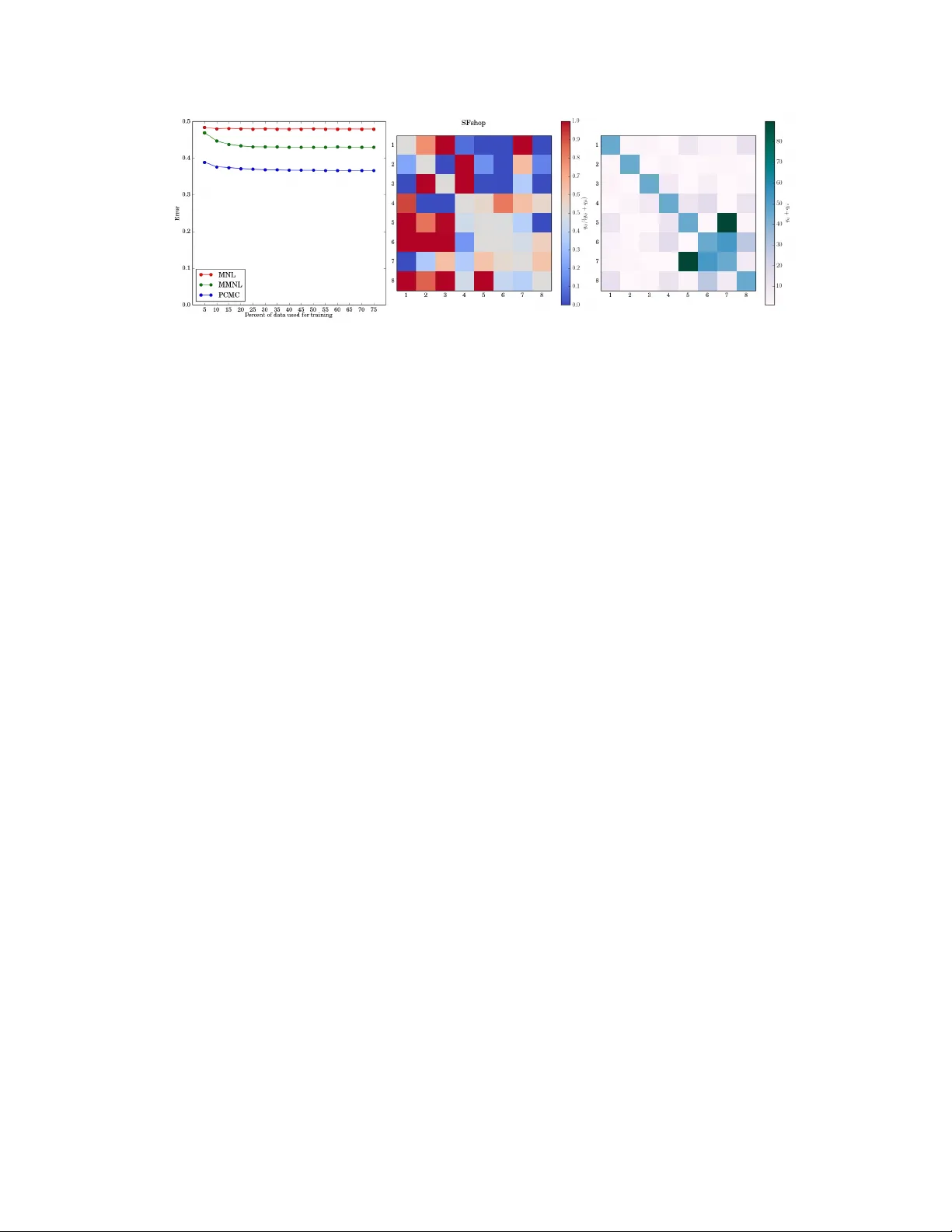
Pairwise Choice Mark ov Chains Stephen Ragain Management Science & Engineering Stanford Univ ersity Stanford, CA 94305 sragain@stanford.edu Johan Ugander Management Science & Engineering Stanford Univ ersity Stanford, CA 94305 jugander@stanford.edu Abstract As datasets capturing human choices gro w in richness and scale—particularly in online domains—there is an increasing need for choice models that escape tra- ditional choice-theoretic axioms such as regularity , stochastic transitivity , and Luce’ s choice axiom. In this work we introduce the Pairwise Choice Markov Chain (PCMC) model of discrete choice, an inferentially tractable model that does not assume any of the abov e axioms while still satisfying the foundational axiom of uniform expansion , a considerably weaker assumption than Luce’ s choice ax- iom. W e show that the PCMC model significantly outperforms both the Multino- mial Logit (MNL) model and a mixed MNL (MMNL) model in prediction tasks on both synthetic and empirical datasets known to exhibit violations of Luce’ s axiom. Our analysis also synthesizes sev eral recent observations connecting the Multinomial Logit model and Marko v chains; the PCMC model retains the Multi- nomial Logit model as a special case. 1 Introduction Discrete choice models describe and predict decisions between distinct alternati ves. T raditional ap- plications include consumer purchasing decisions, choices of schooling or employment, and com- muter choices for modes of transportation among av ailable options. Early models of probabilistic discrete choice, including the well kno wn Thurstone Case V model [ 29 ] and Bradley-T erry-Luce (BTL) model [ 7 ], were dev eloped and refined under diverse strict assumptions about human de- cision making. As complex individual choices become increasingly mediated by engineered and learned platforms—from online shopping to web browser clicking to interactions with recommen- dation systems—there is a pressing need for flexible models capable of describing and predicting nuanced choice behavior . Luce’ s choice axiom, popularly known as the independence of irr elevant alternatives (IIA), is ar- guably the most storied assumption in choice theory [ 20 ]. The axiom consists of tw o statements, ap- plied to each subset of alternati ves S within a broader universe U . Let p aS = Pr( a chosen from S ) for any S ⊆ U , and in a slight abuse of notation let p ab = Pr( a chosen from { a, b } ) when there are only two elements. Luce’ s axiom is then that: (i) if p ab = 0 then p aS = 0 for all S containing a and b , (ii) the probability of choosing a from U conditioned on the choice lying in S is equal to p aS . The BTL model, which defines p ab = γ a / ( γ a + γ b ) for latent “quality” parameters γ i > 0 , satisfies the axiom while Thurstone’ s Case V model does not [ 1 ]. Soon after its introduction, the BTL model was generalized from pairwise choices to choices from larger sets [ 4 ]. The resulting Multinomal Logit (MNL) model again employs quality parameters γ i ≥ 0 for each i ∈ U and defines p iS , the probability of choosing i from S ⊆ U , proportional to γ i for all i ∈ S . Any model that satisfies Luce’ s choice axiom is equivalent to some MNL model [ 21 ]. One consequence of Luce’ s choice axiom is strict stoc hastic tr ansitivity between alternati ves: if p ab ≥ 0 . 5 and p bc ≥ 0 . 5 , then p ac ≥ max( p ab , p bc ) . A possibly undesirable consequence of strict stochastic transitivity is the necessity of a total order across all elements. But note that strict 30th Conference on Neural Information Processing Systems (NIPS 2016), Barcelona, Spain. stochastic transitivity does not imply the choice axiom; Thurstone’ s model exhibits strict stochastic transitivity . Many choice theorists and empiricists, including Luce, ha ve noted that the choice axiom and stochas- tic transiti vity are strong assumptions that do not hold for empirical choice data [ 10 , 14 , 15 , 28 , 30 ]. A range of discrete choice models striving to escape the confines of the choice axiom hav e emerged ov er the years. The most popular of these models hav e been Elimination by Aspects [ 31 ], mixed MNL (MMNL) [ 6 ], and nested MNL [ 24 ]. Inference is practically difficult for all three of these models [ 17 , 25 ]. Additionally , Elimination by Aspects and the MMNL model also both exhibit the rigid property of regularity , defined below . A broad, important class of models in the study of discrete choice is the class of random utility models (R UMs) [ 4 , 22 ]. A R UM af filiates with each i ∈ U a random v ariable X i and defines for each subset S ⊆ U the probability Pr( i chosen from S ) = Pr( X i ≥ X j , ∀ j ∈ S ). An independent RUM has independent X i . R UMs assume neither choice axiom nor stochastic transitivity . Thurstone’ s Case V model and the BTL model are both independent R UMs; the Elimination by Aspects and MMNL models are both R UMs. A major result by McFadden and Train establishes that for any R UM there exists a MMNL model that can approximate the choice probabilities of that R UM to within an arbitrary error [ 25 ], a strong result about the generality of MMNL models. The nested MNL model, meanwhile, is not a R UM. Although R UMs need not exhibit stochastic transitivity , the y still e xhibit the weaker property of r e gularity : for any choice sets A , B where A ⊆ B , p xA ≥ p xB . Regularity may at first seem intuitiv ely pleasing, b ut it prev ents models from e xpressing framing ef fects [ 14 ] and other empirical observations from modern behavior economics [ 30 ]. This rigidity motiv ates us to contribute a new model of discrete choice that escapes historically common assumptions while still furnishing enough structure to be inferentially tractable. The pr esent work. In this work we introduce a conceptually simple and inferentially tractable model of discrete choice that we call the PCMC model. The parameters of the PCMC model are the off-diagonal entries of a rate matrix Q index ed by U . The PCMC model affiliates each subset S of the alternativ es with a continuous time Mark ov chain (CTMC) on S with transition rate matrix Q S , whose off-diagonal entries are entries of Q indexed by pairs of items in S . The model defines p iS , the selection probability of alternati ve i ∈ S , as the probability mass of alternativ e i ∈ S of the stationary distribution of the CTMC on S . The transition rates of these CTMCs can be interpreted as measures of preferences between pairs of alternativ es. Special cases of the model use pairwise choice probabilities as transition rates, and as a result the PCMC model extends arbitrary models of pairwise choice to models of set- wise choice. Indeed, we show that when the matrix Q is parameterized with the pairwise selection probabilities of a BTL pairwise choice model, the PCMC model reduces to an MNL model. Recent parameterizations of non-transitiv e pairwise probabilities such as the Blade-Chest model [ 8 ] can be usefully employed to reduce the number of free parameters of the PCMC model. Our PCMC model can be thought of as building upon the observ ation underlying the recently in- troduced Iterati ve Luce Spectral Ranking (I-LSR) procedure for efficiently finding the maximum likelihood estimate for parameters of MNL models [ 23 ]. The analysis of I-LSR is precisely analyz- ing a PCMC model in the special case where the matrix Q has been parameterized by BTL. In that case the stationary distribution of the chain is found to satisfy the stationary conditions of the MNL likelihood function, establishing a strong connection between MNL models and Markov chains. The PCMC model generalizes that connection. Other recent connections between the MNL model and Markov chains include the work on Rank- Centrality [ 26 ], which employs a discrete time Markov chain for inference in the place of I-LSR’ s continuous time chain, in the special case where all data are pairwise comparisons. Separate recent work has contributed a different discrete time Markov chain model of “choice sub- stitution” capable of approximating any RUM [ 3 ], a related problem but one with a strong focus on ordered preferences. Lastly , recent work by Kumar et al. explores conditions under which a prob- ability distribution ov er discrete items can be expressed as the stationary distribution of a discrete time Markov chain with “score” functions similar to the “quality” parameters in an MNL model [ 19 ]. 2 The PCMC model is not a R UM, and in general does not exhibit stochastic transitivity , regularity , or the choice axiom. W e find that the PCMC model does, howe ver , obey the lesser known but fundamental axiom of uniform expansion , a weakened version of Luce’ s choice axiom proposed by Y ellott that implies the choice axiom for independent R UMs [ 32 ]. In this work we define a con venient structural property termed contractibility , for which uniform e xpansion is a special case, and we show that the PCMC model exhibits contractibility . Of the models mentioned above, only Elimination by Aspects exhibits uniform expansion without being an independent R UM. Elimination by Aspects obe ys regularity , which the PCMC model does not; as such, the PCMC model is uniquely positioned in the literature of axiomatic discrete choice, minimally satisfying uniform expansion without the other aforementioned axioms. After presenting the model and its properties, we in vestigate choice predictions from our model on two empirical choice datasets as well as div erse synthetic datasets. The empirical choice datasets concern transportation choices made on commuting and shopping trips in San Francisco. Inference on synthetic data sho ws that PCMC is competiti ve with MNL when Luce’ s choice axiom holds, while PCMC outperforms MNL when the axiom does not hold. More significantly , for both of the empirical datasets we find that a learned PCMC model predicts empirical choices significantly better than a learned MNL model. 2 The PCMC model a b c a b b c a c Figure 1: Markov chains on choice sets { a, b } , { a, c } , and { b, c } , where line thicknesses denote tran- sition rates. The chain on the choice set { a, b, c } is assembled using the same rates. A Pairwise Choice Markov Chain (PCMC) model defines the selection probability p iS , the probability of choosing i from S ⊆ U , as the probability mass on alternati ve i ∈ S of the stationary distribution of a continuous time Markov chain (CTMC) on the set of alternativ es S . The model’ s parame- ters are the of f-diagonal entries q ij of rate matrix Q indexed by pairs of elements in U . See Figure 1 for a diagram. W e impose the constraint q ij + q j i ≥ 1 for all pairs ( i, j ) , which ensures irreducibility of the chain for all S . Giv en a query set S ⊆ U , we construct Q S by restricting the ro ws and columns of Q to elements in S and setting q ii = − P j ∈ S \ i q ij for each i ∈ S . Let π S = { π S ( i ) } i ∈ S be the stationary distribution of the corresponding CTMC on S , and let π S ( A ) = P x ∈ A π S ( x ) . W e define the choice probability p iS := π S ( i ) , and now sho w that the PCMC model is well defined. Proposition 1. The choice pr obabilities p iS ar e well defined for all i ∈ S , all S ⊆ U of a finite U . Pr oof. W e need only to sho w that there is a single closed communicating class. Because S is finite, there must be at least one closed communicating class. Suppose the chain had more than one closed communicating class and that i ∈ S and j ∈ S were in different closed communicating classes. But q ij + q j i ≥ 1 , so at least one of q ij and q j i is strictly positi ve and the chain can switch communicating classes through the transition with strictly positiv e rate, a contradiction. While the support of π S is the single closed communicating class, S may ha ve transient states corresponding to alternativ es with selection probability 0. Note that irreducibility argument needs only that q ij + q j i be positiv e, not necessarily at least 1 as imposed in the model definition. One could simply constrain q ij + q j i ≥  for some positive  . Ho wev er , multiplying all entries of Q by some c > 0 does not affect the stationary distrib ution of the corresponding CTMC, so multiplication by 1 / gi ves a Q with the same selection probabilities. In the subsections that follow , we dev elop key properties of the model. W e begin by showing how assigning Q according a Bradley-T erry-Luce (BTL) pairwise model results in the PCMC model being equiv alent to BTL ’ s canonical extension, the Multinomial Logit (MNL) set-wise model. W e then construct a Q for which the PCMC model is neither re gular nor a R UM. 2.1 Multinomial Logit from Bradley-T erry-Luce W e now observe that the Multinomial Logit (MNL) model, also called the Plackett-Luce model, is precisely a PCMC model with a matrix Q consisting of pairwise BTL probabilities. Recall that the BTL model assumes the existence of latent “quality” parameters γ i > 0 for i ∈ U with p ij = γ i / ( γ i + γ j ) , ∀ i, j ∈ U and that the MNL generalization defines p iS ∝ γ i , ∀ i ∈ S for each S ⊆ U . 3 Proposition 2. Let γ be the parameter s of a BTL model on U . F or q j i = γ i γ i + γ j , the PCMC pr obabilities p iS ar e consistent with an MNL model on S with parameters γ . Pr oof. W e aim to sho w that π S = γ || γ || 1 is a stationary distrib ution of the PCMC chain: π T S Q S = 0 . W e hav e: ( π T S Q S ) i = 1 || γ || 1   X j 6 = i γ j q j i − γ i ( X j 6 = i q j i )   = γ i || γ || 1   X j 6 = i γ j γ i + γ j − X j 6 = i γ j γ i + γ j   = 0 , ∀ i. Thus π S is always the stationary distribution of the chain, and we know by Proposition 1 that it is unique. It follows that p iS ∝ γ i for all i ∈ S , as desired. Other parameterizations of Q , which can be used for parameter reduction or to extend arbitrary models for pairwise choice, are explored section 1 of the Supplementary material. 2.2 A counterexample to r egularity The regularity property stipulates that for any S 0 ⊂ S , the probability of selecting a from S 0 is at least the probability of selecting a from S . All RUMs exhibit regularity because S 0 ⊆ S implies Pr( X i = max j ∈ S 0 X j ) ≥ Pr( X i = max j ∈ S X j ) . W e now construct a simple PCMC model which does not exhibit re gularity , and is thus not a RUM. Consider U = { r, p, s } corresponding to a rock-paper-scissors-like stochastic game where each pairwise matchup has the same win probability α > 1 2 . Constructing a PCMC model where the transition rate from i to j is α if j beats i in rock-paper-scissors yields the rate matrix Q = " − 1 1 − α α α − 1 1 − α 1 − α α − 1 # . W e see that for pairs of objects, the PCMC model returns the same probabilities as the pairwise game, i.e. p ij = α when i beats j in rock-paper-scissors, as p ij = q j i when q ij + q j i = 1 . Regardless of how the probability α is chosen, howe ver , it is always the case that p rU = p pU = p sU = 1 / 3 . It follows that re gularity does not hold for α > 2 / 3 . W e view the PCMC model’ s lack of regularity is a positiv e trait in the sense that empirical choice phenomena such as framing effects and asymmetric dominance violate regularity [ 14 ], and the PCMC model is rare in its ability to model such choices. Deriving necessary and suf ficient con- ditions on Q for a PCMC model to be a RUM, analogous to known characterization theorems for R UMs [ 11 ] and kno wn sufficient conditions for nested MNL models to be R UMs [ 5 ], is an interest- ing open challenge. 3 Properties While we ha ve demonstrated already that the PCMC model av oids se veral restricti ve properties that are often inconsistent with empirical choice data, we demonstrate in this section that the PCMC model still exhibits deep structure in the form of contractibility , which implies uniform expansion. Inspired by a thought experiment that was posed as an early challenge to the choice axiom, we define the property of contractibility to handle notions of similarity between elements. W e demonstrate that the PCMC model exhibits contractibility , which gracefully handles this thought experiment. 3.1 Uniform expansion Y ellott [ 32 ] introduced uniform expansion as a weaker condition than Luce’ s choice axiom, but one that implies the choice axiom in the context of any independent RUM. Y ellott posed the axiom of in variance to uniform expansion in the context of “copies” of elements which are “identical. ” In the context of our model, such copies would ha ve identical transition rates to alternati ves: Definition 1 (Copies) . F or i, j in S ⊆ U , we say that i and j ar e copies if for all k ∈ S − i − j , q ik = q j k and q ij = q j i . 4 Y ellott’ s introduction to uniform e xpansion asks the reader to consider an offer of a choice of be ver- age from k identical cups of coffee, k identical cups of tea, and k identical glasses of milk. Y ellott contends that the probability the reader chooses a type of bev erage (e.g. coffee) in this scenario should be the same as if they were only sho wn one cup of each bev erage type, regardless of k ≥ 1 . Definition 2 (Uniform Expansion) . Consider a choice between n elements in a set S 1 = { i 11 , . . . , i n 1 } , and another choice fr om a set S k containing k copies of each of the n elements: S k = { i 11 , . . . , i 1 k , i 21 , . . . , i 2 k , . . . , i n 1 , . . . , i nk } . The axiom of uniform expansion states that for each m = 1 , . . . , n and all k ≥ 1 : p i m 1 S 1 = k X j =1 p i mj S k . W e will show that the PCMC model always exhibits a more general property of contractibility , of which uniform expansion is a special case; it thus alw ays exhibits uniform expansion. Y ellott showed that for an y independent R UM with | U | ≥ 3 the double-exponential distrib ution family is the only family of independent distributions that exhibit uniform expansion for all k ≥ 1 , and that Thurstone’ s model based on the Gaussian distribution family in particular does not exhibit uniform expansion. While uniform e xpansion seems natural in man y discrete choice contexts, it should be re garded with some skepticism in applications that model competitions. Sports matches or races are often modeled using R UMs, where the winner of a competition can be modeled as the competitor with the best draw from their random variable. If a competitor has a performance distribution with a heavy upper tail (so that their wins come from occasional “good days”), uniform expansion would not hold. This observation relates to recent work on team performance and selection [ 16 ], where non-in variance under uniform expansion plays a ke y role. 3.2 Contractibility In a book revie w of Luce’ s early work on the choice axiom, Debreu [ 10 ] considers a hypothetical choice between three musical recordings: one of Beethoven’ s eighth symphony conducted by X , another of Beethoven’ s eighth symphony conducted by Y , and one of Debussy quartet conducted by Z . W e will call these options B 1 , B 2 , and D respectiv ely . When compared to D , Debreu argues that B 1 and B 2 are indistinguishable in the sense that p DB 1 = p DB 2 . Ho wev er , someone may prefer B 1 ov er B 2 in the sense that p B 1 B 2 > 0 . 5 . This is impossible under a BTL model, in which p DB 1 = p DB 2 implies that γ B 1 = γ B 2 and in turn p B 1 B 2 = 0 . 5 . T o address contexts in which elements compare identically to alternati ves b ut not each other (e.g. B 1 and B 2 ), we introduce contr actible partitions that group these similar alternativ es into sets. W e then show that when a PCMC model contains a contractible partition, the relative probabilities of selecting from one of these partitions is independent from ho w comparisons are made between alternativ es in the same set. Our contractible partition definition can be vie wed as akin to (b ut distinct from) nests in nested MNL models [ 24 ]. Definition 3 (Contractible Partition) . A partition of U into non-empty sets A 1 , . . . , A k is a con- tractible partition if q a i a j = λ ij for all a i ∈ A i , a j ∈ A j for some Λ = { λ ij } for i, j ∈ { 1 , . . . , k } . Proposition 3. F or a given Λ , let A 1 , . . . , A k be a contractible partition for two PCMC models on U r epresented by Q, Q 0 with stationary distributions π, π 0 . Then for any A i : X j ∈ A i p j U = X j ∈ A i p 0 j U , (1) or equivalently , π ( A i ) = π 0 ( A i ) . Pr oof. Suppose Q has contractible partition A 1 , . . . , A k with respect to Λ . If we decompose the balance equations (i.e. each row of π T Q = 0 ), for x ∈ A 1 WLOG we obtain: π ( x )   X y ∈ A 1 \ x q xy + k X i =2 X a i ∈ A i q xa i   = X y ∈ A 1 \ x π ( y ) q y x + k X i =2 X a i ∈ A i π ( a i ) q a i x . (2) 5 Noting that for a i ∈ A i and a j ∈ A j , q a i a j = λ ij , ( 2 ) can be rewritten: π ( x )   X y ∈ A 1 \ x q xy   + π ( x ) k X i =2 | A i | λ i 1 = X y ∈ A 1 \ x π ( y ) q y x + k X i =2 π ( A i ) λ i 1 . Summing ov er x ∈ A 1 then giv es X x ∈ A 1 π ( x )   X y ∈ A 1 \ x q xy   + π ( A 1 ) k X i =2 | A i | λ i 1 = X x ∈ A 1 X y ∈ A 1 \ x π ( y ) q y x + | A 1 | k X i =2 π ( A i ) λ i 1 . The leftmost term of each side is equal, so we hav e π ( A 1 ) = | A 1 | P k i =2 π ( A i ) λ i 1 P i =2 | A i | λ 1 i , (3) which mak es π ( A 1 ) the solution to global balance equations for a dif ferent continuous time Marko v chain with the states { A 1 , . . . , A k } and transition rate ˜ q A i A j = | A j | λ ij between state A i and A j , and ˜ q A i A i = − P j 6 = i ˜ q A i A j . Now q a i a j + q a j a i ≥ 1 implies λ ij + λ j i ≥ 1 . Combining this observation with | A i | > 0 shows (as with the proof of Proposition 1) that this chain is irreducible and thus that { π ( A i ) } k i =1 are well-defined. Furthermore, because ˜ Q is determined entirely by Λ and | A 1 | , . . . , | A k | , we ha ve that ˜ Q = ˜ Q 0 , and thus that π ( A i ) = π 0 ( A i ) , ∀ i regardless of ho w Q and Q 0 may differ , completing the proof. The intuition is that we can “contract” each A i to a single “type” because the probability of choosing an element of A i is independent of the pairwise probabilities between elements within the sets. The abov e proposition and the contractibility of a PCMC model on all uniformly expanded sets implies that all PCMC models exhibit uniform e xpansion. Proposition 4. Any PCMC model exhibits uniform e xpansion. Pr oof. W e translate the problem of uniform expansion into the language of contractibility . Let U 1 be the univ erse of unique items i 11 , i 21 , . . . , i n 1 , and let U k be a univ erse containing k copies of each item in U 1 . Let i mj denote the j th copy of the m th item in U 1 . Thus U k = ∪ n m =1 ∪ k j =1 i mj . Let Q be the transition rate matrix of the CTMC on U 1 . W e construct a contractible partition of U k into the n sets, each containing the k copies of some item in U 1 . Thus A m = ∪ k j =1 i mj . By the definition of copies, that { A m } n m =1 is a contractible partition of U k with Λ = Q . Noting | A m | = k for all m in Equation ( 3 ) abov e results in { π ( A m ) } n m =1 being the solution to π T Q = π T Λ = 0 . Thus p i m U 1 = π ( A m ) = P k j =1 p i mj U k for each m , sho wing that the model exhibits uniform expansion. W e end this section by noting that e very PCMC model has a trivial contractible partition into single- tons. Detection and exploitation of Q ’ s non-trivial contractible partitions (or appropriately defined “nearly contractible partitions”) are interesting open research directions. 4 Inference and pr ediction Our ultimate goal in formulating this model is to make predictions: using past choices from diverse subsets S ⊆ U to predict future choices. In this section we first giv e the log-likelihood function log L ( Q ; C ) of the rate matrix Q given a choice data collection of the form C = { ( i k , S k ) } n k =1 , where i k ∈ S k was the item chosen from S k . W e then inv estigate the ability of a learned PCMC model to make choice predictions on empirical data, benchmarked ag ainst learned MNL and MMNL models, and interpret the inferred model parameters ˆ Q . Let C iS ( C ) = |{ ( i k , S k ) ∈ C : i k = i, S k = S }| denote the number of times in the data that i was chosen out of set S for each S ⊆ U , and let C S ( C ) = |{ ( i k , S k ) ∈ C : S k = S }| be the number of times that S was the choice set for each S ⊆ U . 6 4.1 Maximum likelihood For each S ⊆ U , i ∈ S , recall that p iS ( Q ) is the probability that i is selected from set S as a function of the rate matrix Q . After dropping all additive constants, the log-likelihood of Q given the data C (deriv ed from the probability mass function of the multinomial distribution) is: log L ( Q ; C ) = X S ⊆ U X i ∈ S C iS ( C ) log( p iS ( Q )) . Recall that for the PCMC model, p iS ( Q ) = π S ( i ) , where π S is the stationary distribution for a CTMC with rate matrix Q S , i.e. π T S Q S = 0 and P i ∈ S π S ( i ) = 1 . There is no general closed form expression for p iS ( Q ) . The implicit definition also makes it difficult to derive gradients for log L with respect to the parameters q ij . W e employ SLSQP [ 27 ] to maximize log L ( Q ; C ) , which is non- concav e in general. For more information on the optimization techniques used in this section, see the Supplementary Materials. 4.2 Empirical data results W e ev aluate our inference procedure on two empirical choice datasets, SFwork and SFshop , col- lected from a surve y of transportation preferences around the San Francisco Bay Area [ 18 ]. The SFshop dataset contains 3,157 observations each consisting of a choice set of transportation alter- nativ es a v ailable to individuals trav eling to and returning from a shopping center , as well as a choice from that choice set. The SFwork dataset, meanwhile, contains 5,029 observ ations consisting of commuting options and the choice made on a gi ven commute. Basic statistics describing the choice set sizes and the number of times each pair of alternativ es appear in the same choice set appear in the Supplementary Materials 1 . W e train our model on observations T train ⊂ C and ev aluate on a test set T test ⊂ C via Error ( T train ; T test ) = 1 | T test | X ( i,S ) ∈ T test X j ∈ S | p j S ( ˆ Q ( T train )) − ˜ p iS ( T test ) | , (4) where ˆ Q ( T train ) is the estimate for Q obtained from the observations in T train and ˜ p iS ( T test ) = C iS ( T test ) /C S ( T test ) is the empirical probability of i was selected from S among observations in T test . Note that Error ( T train ; T test ) is the expected ` 1 -norm of the difference between the empirical distribution and the inferred distribution on a choice set drawn uniformly at random from the obser - vations in T test . W e applied small amounts of additive smoothing to each dataset. W e compare our PCMC model against both an MNL model trained using Iterativ e Luce Spectral Ranking (I-LSR) [ 23 ] and a more flexible MMNL model. W e used a discrete mixture of k MNL models (with O ( k n ) parameters), choosing k so that the MMNL model had strictly more parameters than the PCMC model on each data set. For details on how the MMNL model was trained, see the Supplementary Materials. Figure 3 shows Error ( T train ; T test ) on the SFwork data as the learning procedure is applied to in- creasing amounts of data. The results are averaged over 1,000 dif ferent permutations of the data with a 75/25 train/test split employed for each permutation. W e sho w the error on the testing data as we train with increasing proportions of the training data. A similar figure for SFshop data appears in the Supplementary Materials. W e see that our model is better equipped to learn from and make predictions in both datasets, and when using all of the training data, we observe an error reduction of 36.2% and 46.5% compared to MNL and 24.4% and 31.7% compared to MMNL on SFwork and SFshop respectiv ely . Figure 3 also gives two different heat maps of ˆ Q for the SFwork data, showing the relativ e rates ˆ q ij / ˆ q j i between pairs of items as well as how the total rate ˆ q ij + ˆ q j i between pairs compares to total rates between other pairs. The index ordering of each matrix follows the estimated selection probabilities of the PCMC model on the full set of the alternati ves for that dataset. The ordered options for SFwork are: (1) driving alone, (2) sharing a ride with one other person, (3) walking, 1 Data and code av ailable here: https://github.com/sragain/pcmc-nips 7 Figure 2: Prediction error on a 25% holdout of the SFwork data for the PCMC, MNL, and MMNL models. PCMC sees improvements of 34.1% and 23.1% in prediction error over MNL and MMNL, respectiv ely , when training on 75% of the data. (4) public transit, (5) biking, and (6) carpooling with at least two others. Numerical values for the entries of ˆ Q for both datasets appear in the Supplementary Materials. The inferred pairwise selection probabilities are ˆ p ij = ˆ q j i / ( ˆ q j i + ˆ q ij ) . Constructing a tournament graph on the alternativ es where ( i, j ) ∈ E if ˆ p ij ≥ 0 . 5 , cyclic triplets are then length-3 c ycles in the tournament. A bound due to Harary and Moser [ 13 ] establishes that the maximum number of c yclic triples on a tournament graph on n nodes is 8 when n = 6 and 20 when n = 8 . According to our learned model, the choices exhibit 2 out of a maximum 8 cyclic triplets in the SFwork data and 6 out of a maximum 20 cyclic triplets for the SFshop data. Additional ev aluations of predictiv e performance across a range of synthetic datasets appear in the Supplementary Materials. The majority of datasets in the literature on discrete choice focus on pairwise comparisons or ranked lists, where lists inherently assume transiti vity and the independence of irrelev ant alternatives. The SFwork and SFshop datasets are rare examples of public datasets that genuinely study choices from sets larger than pairs. 5 Conclusion W e introduce a P airwise Choice Marko v Chain (PCMC) model of discrete choice which defines selection probabilities according to the stationary distributions of continuous time Markov chains on alternativ es. The model parameters are the transition rates between pairs of alternatives. In general the PCMC model is not a random utility model (RUM), and maintains broad flexibility by eschewing the implications of Luce’ s choice axiom, stochastic transitivity , and re gularity . De- spite this flexibility , we demonstrate that the PCMC model exhibits desirable structure by fulfilling uniform expansion, a property previously found only in the Multinomial Logit (MNL) model and the intractable Elimination by Aspects model. W e also introduce the notion of contractibility , a property motiv ated by thought experiments instru- mental in moving choice theory beyond the choice axiom, for which Y ellott’ s axiom of uniform expansion is a special case. Our work demonstrates that the PCMC model exhibits contractibility , which implies uniform expansion. W e also showed that the PCMC model of fers straightforward in- ference through maximum likelihood estimation, and that a learned PCMC model predicts empirical choice data with a significantly higher fidelity than both MNL and MMNL models. The flexibility and tractability of the PCMC model opens up many compelling research directions. First, what necessary and sufficient conditions on the matrix Q guarantee that a PCMC model is a R UM [ 11 ]? The efficacy of the PCMC model suggests exploring other effecti ve parameterizations for Q , including developing inferential methods which exploit contractibility . There are also open computational questions, such as streamlining the likelihood maximization using gradients of the implicit function definitions. V ery recently , learning results for nested MNL models hav e shown fa vorable query complexity under an oracle model [ 2 ], and a comparison of our PCMC model with these approaches to learning nested MNL models is important future work. Acknowledgements. This work was supported in part by a David Mor genthaler II F aculty Fellow- ship and a Dantzig–Lieberman Operations Research Fellowship. W e thank Flavio Chierichetti and 8 Ravi Kumar for noticing an irregularity in the previously published version of Figure 4 that helped us identify a minor bug. Figures 3 and 4 hav e been fixed in this arxi v version. References [1] E. Adams and S. Messick. An axiomatic formulation and generalization of successiv e intervals scaling. Psychometrika , 23(4):355–368, 1958. [2] A. R. Benson, R. Kumar , and A. T omkins. On the rele vance of irrele vant alternati ves. In WWW , 2016. [3] J. Blanchet, G. Gallego, and V . Goyal. A markov chain approximation to choice modeling. In EC , 2013. [4] H. D. Block and J. Marschak. Random orderings and stochastic theories of responses. Contributions to Pr obability and Statistics , 2:97–132, 1960. [5] A. B ¨ orsch-Supan. On the compatibility of nested logit models with utility maximization. Journal of Econometrics , 43(3):373–388, 1990. [6] J H Boyd and R E Mellman. The effect of fuel economy standards on the us automoti ve market: an hedonic demand analysis. T ransportation Resear ch P art A: General , 14(5-6):367–378, 1980. [7] R. A. Bradley and M. E. T erry . Rank analysis of incomplete block designs the method of paired compar- isons. Biometrika , 39(3-4):324–345, 1952. [8] S. Chen and T . Joachims. Modeling intransitivity in matchup and comparison data. In WSDM , 2016. [9] Shuo Chen and Thorsten Joachims. Predicting matchups and preferences in context. In Pr oceedings of the 22Nd A CM SIGKDD International Confer ence on Knowledg e Discovery and Data Mining , KDD ’16, pages 775–784, New Y ork, NY , USA, 2016. A CM. [10] G. Debreu. Re view of individual choice behavior: A theoretical analysis. American Economic Revie w , 1960. [11] J.-C. Falmagne. A representation theorem for finite random scale systems. J. Math. Psych. , 18(1):52–72, 1978. [12] P . E. Green, A. M. Krieger , and Y . Wind. Thirty years of conjoint analysis: Reflections and prospects. Interfaces , 31(3 supplement):S56–S73, 2001. [13] Frank Harary and Leo Moser . The theory of round robin tournaments. The American Mathematical Monthly , 73(3):231–246, 1966. [14] J. Huber , J. W . Payne, and C. Puto. Adding asymmetrically dominated alternati ves: V iolations of regular - ity and the similarity hypothesis. Journal of Consumer Resear ch , pages 90–98, 1982. [15] S. Ieong, N. Mishra, and O. Sheffet. Predicting preference flips in commerce search. In ICML , 2012. [16] J. Kleinberg and M. Raghu. T eam performance with test scores. In EC , pages 511–528, 2015. [17] R. Kohli and K. Jedidi. Error theory for elimination by aspects. Operations Resear ch , 63(3):512–526, 2015. [18] F . S K oppelman and C. Bhat. A self instructing course in mode choice modeling: multinomial and nested logit models. US Department of T ransportation, F ederal T ransit Administration , 31, 2006. [19] Ravi K umar , Andre w T omkins, Ser gei V assilvitskii, and Erik V ee. In verting a steady-state. In Proceedings of the Eighth ACM International Conference on W eb Searc h and Data Mining , pages 359–368. A CM, 2015. [20] R. D. Luce. Individual Choice Behavior: A Theoretical Analysis . Wile y , 1959. [21] R. D. Luce. The choice axiom after twenty years. J. Math. Psyc h. , 15(3):215–233, 1977. [22] C. F . Manski. The structure of random utility models. Theory and Decision , 8(3):229–254, 1977. [23] L. Maystre and M. Grossglauser . Fast and accurate inference of plackett–luce models. In NIPS , 2015. [24] D. McFadden. Econometric models for probabilistic choice among products. Journal of Business , pages S13–S29, 1980. [25] D. McFadden, K. T rain, et al. Mixed mnl models for discrete response. Journal of Applied Econometrics , 15(5):447–470, 2000. [26] S. Negahban, S. Oh, and D. Shah. Rank centrality: Ranking from pair-wise comparisons. arXiv preprint arXiv:1209.1688v4 , 2015. [27] J. Nocedal and S. J. Wright. Numerical optimization. 2006. [28] I. Simonson and A. Tversky . Choice in context: Tradeof f contrast and extremeness aversion. J ournal of Marketing Resear ch , 29(3):281, 1992. 9 [29] L. L. Thurstone. A law of comparati ve judgment. Psychological Revie w , 34(4):273, 1927. [30] J. S. Trueblood, S. D. Brown, A. Heathcote, and J. R. Busemeyer . Not just for consumers context effects are fundamental to decision making. Psychological Science , 24(6):901–908, 2013. [31] A. Tversky . Elimination by aspects: A theory of choice. Psychological Revie w , 79(4):281, 1972. [32] J. I. Y ellott. The relationship between luce’ s choice axiom, thurstone’ s theory of comparative judgment, and the double exponential distrib ution. J. Math. Psych. , 15(2):109–144, 1977. 10 Supplemental Materials 6 Parameterizations of the Q matrix As observed in the main paper , if we parametrize Q with pairwise probabilities from a BTL model with pa- rameters γ = { γ i } n i =1 , i.e. q ij = p j i = γ j γ i + γ j , the resulting PCMC model is equivalent to an MNL model with parameters γ . In this section we explore some other ways of parameterizing Q via a pairwise probability matrix P with entries p ij and setting Q = P T . Blade-Chest models [ 8 ] are based on geometric d -dimensional embeddings of alternati ves, where each alterna- tiv e i is parameterized with a blade v ector b i ∈ R d and a chest vector c i ∈ R d , in addition to a BTL-like quality parameter γ i > 0 . The Blade-Chest model comes in two variations: the Blade-Chest distance model , where p ij ( b, c, γ ) = S ( || b i − c j || 2 2 − || b j − c i || 2 2 + γ i − γ j ) , where S ( x ) = (1 + exp( − x )) − 1 is the sigmoid/logistic function, and the Blade-Chest inner product model , where p ij ( b, c, γ ) = S ( b i · c j − b j · c i + γ i − γ j ) . The quality parameters γ i serve to connect the models to the BTL model, b ut do not meaningfully increase their expressiv eness, so we disregard them in our use of the Blade-Chest model here. These two Blade-Chest models pro vide useful parameterizations of non-transiti ve pairwise probability matrices, P ( θ ) , with θ = { b, c } consisting of the 2 dn parameters of the “blade” and “chest” embeddings. Another technique for parametrizing Q inv olves representing q ij as a function of features of i and j , i.e. q ij = f ( X i , X j ; θ ) where X i giv es the salient features of i , and θ represents parameters that, for instance, giv e weights to these features. W e can also formulate such analysis as a factoring Q = W T F − D , where W is a weight matrix, F a feature matrix, and D a diagonal matrix ensuring that the row sums of Q are zero. W e do not explore such parameterizations in this work, b ut merely highlight the potential to emplo y latent features of objects in a straight-forward manner, an approach closely related to conjoint analysis [ 12 ]. Such extensions would be similar to Chen and Joachims’ s work exploiting features of pairwise matchups by parametrizing the blades and chests as functions of those features [ 9 ]. 7 Inference with synthetic data W e now ev aluate our inference procedure’ s performance in three synthetic data regimes: (i) choice data gen- erated from a PCMC model with q ij drawn i.i.d. uniformly from [0 , 1] , (ii) choice data generated for a simple MNL model with qualities γ drawn uniformly on the simplex, and (iii) choice data generated from a PCMC model with Q parameterized by a two-dimensional Blade-Chest distance model. In order to create a strongly non-transitiv e instance of the Blade-Chest distance model, we draw the blades b i and chests c i uniformly at i.i.d. points along the two-dimensional unit circle, naturally producing many triadic impasses. The PCMC model’ s Q matrix has n ( n − 1) parameters in general. When Q is parameterized according to BTL we hav e just n parameters, and when it is parameterized according to a Blade-Chest distance model in d dimensions, we hav e 2 dn parameters. W e evaluate each parameterization (arbitrary , MNL, Blade-Chest distance) for each synthetic regime. W e em- ploy the Iterati ve Luce Spectral Ranking (I-LSR) algorithm to learn the model under the BTL parameterization of Q , where the PCMC model is equi v alent to an MNL model. When the data is generated by MNL, we e xpect MNL to outperform inference under the general parameterization. When the data is generated by a non-MNL PCMC model, we e xpect MNL to e xhibit restricted performance compared to a general parameterization, since the data is not generated by a model that MNL can capture. 7.1 Synthetic data results W e generate training data T train and test data T test from each model using 25 randomly chosen triplets as choice sets. W e then follow the inferential procedure in the main paper to ev aluare the inferential efficac y of each of the three models on data generated according to each. Figure 3 sho ws our error performance as the data gro ws, a veraged across 10 instances, for each data generating process and each inference parameterization. W e generate 5000 samples, assign 1000 of these to be testing samples, and incrementally add the other 4000 samples to the training data, tracking error on the testing samples as we increase the size of the training data set. The inference is applied to a set U with n = 10 objects, meaning that MNL has 20 parameters, the PCMC model with arbitrary Q has n ( n − 1) = 90 parameters, and the PCMC model with the Blade-Chest distance pa- rameterization in R 2 uses 2 dn = 40 parameters. Overall we examine 9 data–model pairs, trained sequentially in 5 episodes, av eraged across 10 instances. The figure thus represents 450 trained models. 11 Figure 3: Learning error for PCMC, I-LSR, and Blade-Chest PCMC on synthetic data generated from (i) Arbitrary Q , (ii) MNL, and (iii) Blade-Chest models. As expected, the inferred PCMC models outperform MNL on data exhibiting IIA violations, while the MNL model learns the MNL data better , though PCMC is not far behind. More significantly , the Blade-Chest parametrization of the PCMC model performs very similarly to the general PCMC model in all three sce- narios, despite having far fewer parameters. This is promising in domains where the O ( n 2 ) parameters of a general PCMC model is infeasible but a O ( n ) parameterization using a Blade-Chest representation may be feasible. 8 Additional empirical data results and analysis 8.1 Optimization and smoothing The MNL models were trained using I-LSR, a specialized algorithm for training Multinomial Logit mod- els. Meanwhile, the PCMC likelihood was optimized using SQSLP [ ? ] while the Mixed MNL models were trained using L-BFGS-B [ ? ], which are both general purpose optimization algorithms av ailable as part of the scipy.optimize.minimize software package. The reason for the different choices is that L-BFGS-B does not support the linear constraints that are part of the PCMC model lik elihood. W e choose to use L-BFGS- B for the MMNL model because it outperformed SQSLP on SFtravel data, and we w anted to ensure that we were affording it the best possible chance to do well ag ainst the new model we contrib ute in this work. The additive smoothing applied was α = 0 . 1 for SFwork and α = 5 for SFshop , where α is added to each C iS appearing in the likelihood function. The major motiv ator for the additive smoothing is that SQSLP occasionally goes awry on some of the permutations of the data, maintaining high error after a bad step. Even as currently formulated, the mean error improvement is somewhat underestimating the efficac y of the PCMC model, as a few bad runs out of 1000 will ske w the distribution. Bad runs are easy to identify using cross- validation. Additionally , the implementation of SQSLP would try to compute numerical gradients through function e valuation at points outside the feasible space, which sometimes in v olved q ij + q j i = 0 , violating the irreducibility of the chain. Additiv e smoothing prevents these issues at the cost of some efficacy of the model. W e find the improvement in error of the PCMC model to be ev en more significant in light of the optimization issues in volv ed, and find that it reinforces de velopment of PCMC training algorithms as an interesting research area. Refining the optimization routines for learning PCMC models should be seen as important future work. 8.2 Empirical results f or SFshop data Figure 4 analyzes the SFshop dataset 2 , repeating the analysis of SFwork found in the main paper . The indexing of ˆ Q is again according to the estimated selection probabilities on the full set of alternatives, which were: (1) driv e alone both directions, (2) share a ride with one person in both directions, (3) share a ride with one person in one direction and driv e alone in the other direction, (4) walk, (5) share a ride with more than one person in both directions, (6) share a ride with one person in one direction and more than one in the other direction, (7) bike, and (8) take public transit. The MMNL model here mixes k = 6 models, giving it 48 parameters while PCMC has 56 and MNL has 8. When using the full training set, PCMC performs 31.3% better than MNL and 19.2% better than MMNL. 2 May 2021: The version of Figure 4 that appeared in the NIPS 2016 conference proceedings incorrectly incorporated smoothing of the test data. Fixing this bug, the absolute performance of the models changes somewhat, b ut the relativ e performance and conclusions drawn remain unchanged. 12 Figure 4: Prediction error on SFshop data for the PCMC, MNL, and MMNL models. There are improv ements of 23.1% and 13.9% in prediction error over MNL and MMNL respecti vely when training on 75% of the data. 8.3 Inferred ˆ Q matrices The numerical values of the learned ˆ Q matrices, trained 100% of the data, are given belo w . ˆ Q work =        − 3 . 875 2 . 314 0 . 557 0 . 0 . 1 . 004 18 . 17 − 29 . 571 0 . 776 1 . 836 2 . 075 6 . 713 4 . 84 7 . 752 − 35 . 994 1 . 042 14 . 476 7 . 884 1 . 0 . 105 0 . 456 − 13 . 147 3 . 65 7 . 937 21 . 201 9 . 108 3 . 323 7 . 363 − 47 . 7 6 . 704 11 . 459 3 . 014 0 . 117 5 . 67 12 . 334 − 32 . 594        ˆ Q shop =           − 35 . 264 1 . 0 . 1 . 0 . 0 . 5 . 142 28 . 122 0 . − 12 . 959 3 . 363 0 . 0 . 2 . 03 2 . 433 5 . 133 1 . 635 0 . − 22 . 945 0 . 637 0 . 243 0 . 4 . 877 15 . 553 0 . 12 . 73 5 . 95 − 24 . 455 2 . 174 0 . 1 . 2 . 601 1 . 3 . 487 4 . 458 0 . 194 − 15 . 366 0 . 5 . 227 1 . 1 . 1 . 143 5 . 788 6 . 841 6 . 344 − 31 . 747 6 . 15 4 . 482 1 . 331 1 . 305 0 . 136 0 . 0 . 226 0 . − 30 . 693 27 . 695 0 . 0 . 0 . 402 10 . 521 0 . 0 . 1 . 602 − 12 . 526           8.4 Count matrices Here we present data about the frequency with which pairs of alternati ves appear in the same choice set. Matrices A work and A shop hav e as their ( i, j ) entry the number of choice sets which contained both i and j in the SFwork and SFshop datasets respectiv ely: A work =        − 1323 4755 3729 1658 4755 1323 − 1479 1395 797 1479 4755 1479 − 4003 1738 5029 3729 1395 4003 − 1611 4003 1658 797 1738 1611 − 1738 4755 1479 5029 4003 1738 −        A shop =           − 3075 3075 3075 1844 3075 2069 2916 3075 − 3157 3157 1908 3157 2136 2997 3075 3157 − 3157 1908 3157 2136 2997 3075 3157 3157 − 1908 3157 2136 2997 1844 1908 1908 1908 − 1908 1908 1876 3075 3157 3157 3157 1908 − 2136 2997 2069 2136 2136 2136 1908 2136 − 2094 2916 2997 2997 2997 1876 2997 2094 −           The relativ e frequencies of choice sets of different sizes in the tw o datasets are giv en in T able 1 . 13 T able 1: | S | = 3 4 5 6 7 8 SFwork 948 1918 1461 702 - - SFshop 0 1 131 902 311 1812 14