Unsupervised Deep Clustering for Source Separation: Direct Learning from Mixtures using Spatial Information

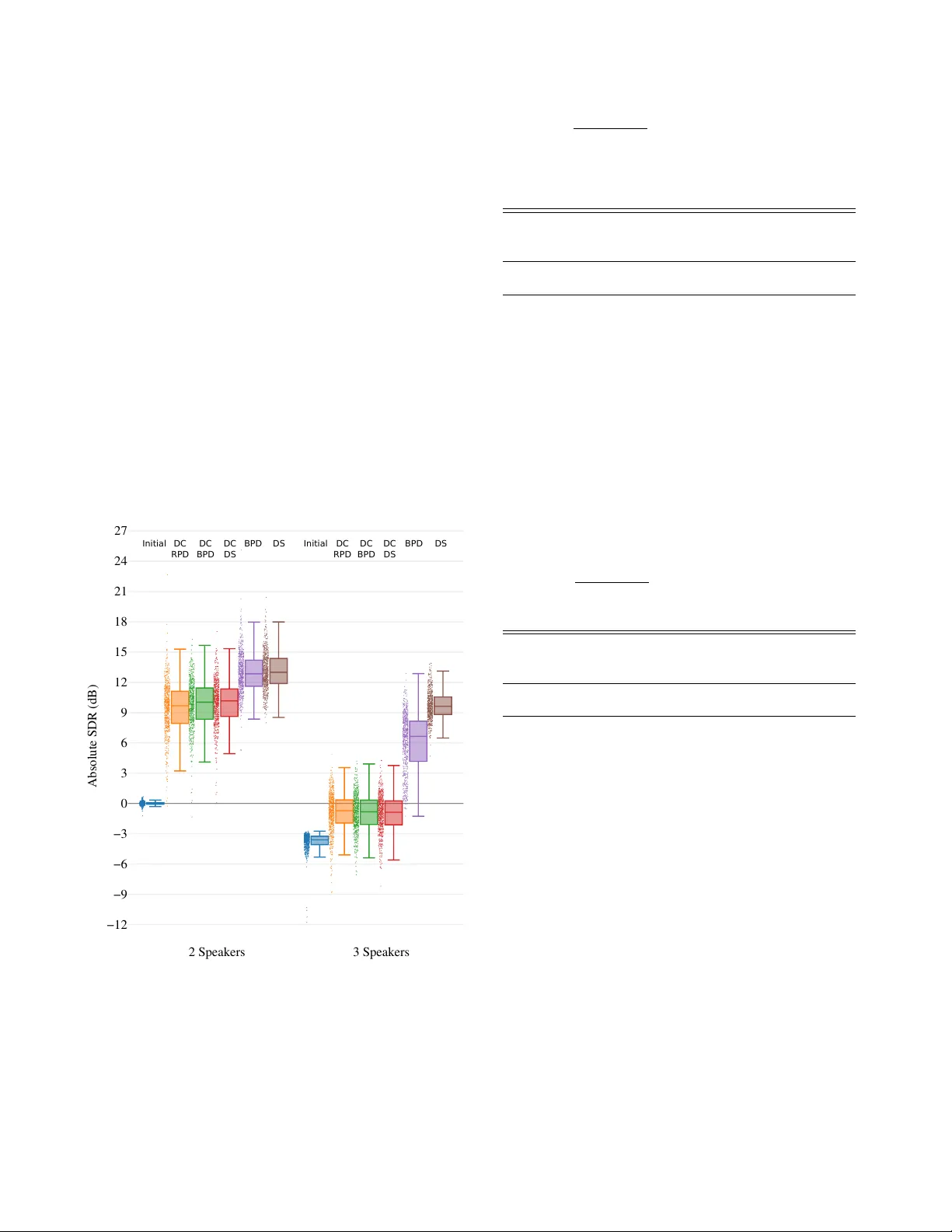
UNSUPER VISED DEEP CLUSTERING FOR SOURCE SEP ARA TION: DIRECT LEARNING FR OM MIXTURES USING SP A TIAL INFORMA TION Efthymios Tzinis ] Shrikant V enkataramani ] P aris Smara gdis ][ ] Uni versity of Illinois at Urbana-Champaign, Department of Computer Science [ Adobe Research ABSTRA CT W e present a monophonic source separation system that is trained by only observing mixtures with no ground truth separation infor- mation. W e use a deep clustering approach which trains on multi- channel mixtures and learns to project spectrogram bins to source clusters that correlate with v arious spatial features. W e show that using such a training process we can obtain separation performance that is as good as making use of ground truth separation information. Once trained, this system is capable of performing sound separation on monophonic inputs, despite having learned how to do so using multi-channel recordings. Index T erms — Deep clustering, source separation, unsuper- vised learning 1. INTR ODUCTION A central problem when designing source separation systems is that of defining what constitutes a source. Multi-microphone systems like [1, 2, 3, 4] make use of spatial information to define and iso- late sources, component-based systems like [5, 6], use pre-learned dictionaries to identify sources, and more recently , neural net-based models [7, 8] learn to identify sources using training examples. Un- less there is some definition of what a source is, performing source separation is not possible. This statement seems incongruous to our own e xperience as listeners. W e grow up listening predominantly to mixtures, and we are able to identify sources e ven in the absence of spatial cues (e.g. multiple sources coming from the same speaker). In this paper we seek to design a system that exhibits the same be- havior . T o do so we aim to answer two questions: First, can we learn source models by only using mixtures with no ground truth source information? And second, can we use that training process in order to learn to perform single-channel source separation? What we find in this paper is that we can indeed learn to identify an open set of sound sources by training on spatial differences from multi-channel mixtures, and that we can transfer that knowledge to a system that can identify and e xtract sources from single-channel mixture record- ings. W e also find that this system works as well as had it been trained with clean data and accurate targets in a traditional manner . T o achiev e our goal, we mak e use of the deep clustering frame- work in [9], because it exhibits the property of generalizing to multi- ple sources. This system learns embeddings of time-frequency bins of mixtures that are projected in distinct clusters corresponding to individual sources. This is ensured by using target labels that assign each input time-frequency bin to a cluster , and an appropriate cost function that finds an embedding that clusters the input similarly to Code: github .com/etzinis/unsupervised spatial dc Supported by NSF grant #1453104 the tar get labels. In our work, we will not make use of user -specified target labels, we will instead use an unsupervised approach where an appropriate embedding will be automatically discovered by forcing it to correlate with features extracted from the presented mixtures during training. Although there is a wide range of such features one can use, in this paper we will make use of inter-microphone phase differences as shown in [10]. W e additionally report results from using labels resulting from clustering these features, and leave it for future experimentation to explore more options. Once trained, this model can be applied on single-channel inputs, and as we show it can match, or even surpass, the performance of an equiv alent model trained on user-pro vided labels. Through this approach we can min- imize the ef fort required to construct training data sets, and instead learn such models by ha ving them listen to multi-channel recordings in the field. 2. INFERRING SOURCE ASSIGNMENTS In this section we show how we make use of spatial information to obtain targets that we can use to train a deep clustering network from mixtures. W e will do so using two instances of a specific representa- tion, but alternativ e features (not necessarily spatial) that also result in source clusters can be used instead. In the following sections we present how we constructed mixtures to test our proposed model, how we extracted the necessary features, and how we can infer a source separation mask. 2.1. Input assumptions W e assume a mixture recording made with 2 microphones that are set close together in the center of a room and N sources in positions P 1 , · · · , P N which are dispersed across the area in fixed positions as shown in Figure 1. W e assume that the microphones are close enough that the maximal time-delay of a source between them will not be more than one sample. Furthermore, in order to hav e some spatial separation of the sources we assume that the angle differ- ence between any two sources would be bigger than ten degrees, i.e., | ∠ ( P i ) − ∠ ( P j ) | > 10 o ∀{ i, j } , i 6 = j . In our experiments we used a sample rate of 16 kHz, and a microphone distance of 1 cm. Let s i ( t ) denote the signal which is emitted from source i while a delayed version of it by τ > 0 would be noted as s i ( t − τ ) . Without any loss of generality , the mixtures that are recorded in both micro- phones ( m 1 ( t ) and m 2 ( t ) ) can be written as: m 1 ( t ) = a 1 · s 1 ( t ) + · · · + a N · s N ( t ) m 2 ( t ) = a 1 · s 1 ( t + δ τ 1 ) + · · · + a N · s N ( t + δ τ N ) (1) where δ τ i denotes the time delay ( δ τ i > 0 ) between the record- ing of the signal s i from the first microphone to the second. The 0  AAAB/HicbVDLSsNAFL2pr1pf8bFzEyyCCymJFNRdwY3LCsYWmlgm00k7dDIJMxOhhuCvuHGh4tYPceffOGmz0NYDA4dz7uWeOUHCqFS2/W1UlpZXVteq67WNza3tHXN3707GqcDExTGLRTdAkjDKiauoYqSbCIKigJFOML4q/M4DEZLG/FZNEuJHaMhpSDFSWuqbB16E1CgIM9s7vc88TAXO875Ztxv2FNYicUpShxLtvvnlDWKcRoQrzJCUPcdOlJ8hoShmJK95qSQJwmM0JD1NOYqI9LNp+tw61srACmOhH1fWVP29kaFIykkU6Mkiq5z3CvE/r5eq8MLPKE9SRTieHQpTZqnYKqqwBlQQrNhEE4QF1VktPEICYaULq+kSnPkvLxL3rHHZcG6a9VazbKMKh3AEJ+DAObTgGtrgAoZHeIZXeDOejBfj3fiYjVaMcmcf/sD4/AHrkJUK AAAB/HicbVDLSsNAFL2pr1pf8bFzEyyCCymJFNRdwY3LCsYWmlgm00k7dDIJMxOhhuCvuHGh4tYPceffOGmz0NYDA4dz7uWeOUHCqFS2/W1UlpZXVteq67WNza3tHXN3707GqcDExTGLRTdAkjDKiauoYqSbCIKigJFOML4q/M4DEZLG/FZNEuJHaMhpSDFSWuqbB16E1CgIM9s7vc88TAXO875Ztxv2FNYicUpShxLtvvnlDWKcRoQrzJCUPcdOlJ8hoShmJK95qSQJwmM0JD1NOYqI9LNp+tw61srACmOhH1fWVP29kaFIykkU6Mkiq5z3CvE/r5eq8MLPKE9SRTieHQpTZqnYKqqwBlQQrNhEE4QF1VktPEICYaULq+kSnPkvLxL3rHHZcG6a9VazbKMKh3AEJ+DAObTgGtrgAoZHeIZXeDOejBfj3fiYjVaMcmcf/sD4/AHrkJUK AAAB/HicbVDLSsNAFL2pr1pf8bFzEyyCCymJFNRdwY3LCsYWmlgm00k7dDIJMxOhhuCvuHGh4tYPceffOGmz0NYDA4dz7uWeOUHCqFS2/W1UlpZXVteq67WNza3tHXN3707GqcDExTGLRTdAkjDKiauoYqSbCIKigJFOML4q/M4DEZLG/FZNEuJHaMhpSDFSWuqbB16E1CgIM9s7vc88TAXO875Ztxv2FNYicUpShxLtvvnlDWKcRoQrzJCUPcdOlJ8hoShmJK95qSQJwmM0JD1NOYqI9LNp+tw61srACmOhH1fWVP29kaFIykkU6Mkiq5z3CvE/r5eq8MLPKE9SRTieHQpTZqnYKqqwBlQQrNhEE4QF1VktPEICYaULq+kSnPkvLxL3rHHZcG6a9VazbKMKh3AEJ+DAObTgGtrgAoZHeIZXeDOejBfj3fiYjVaMcmcf/sD4/AHrkJUK AAAB/HicbVDLSsNAFL2pr1pf8bFzEyyCCymJFNRdwY3LCsYWmlgm00k7dDIJMxOhhuCvuHGh4tYPceffOGmz0NYDA4dz7uWeOUHCqFS2/W1UlpZXVteq67WNza3tHXN3707GqcDExTGLRTdAkjDKiauoYqSbCIKigJFOML4q/M4DEZLG/FZNEuJHaMhpSDFSWuqbB16E1CgIM9s7vc88TAXO875Ztxv2FNYicUpShxLtvvnlDWKcRoQrzJCUPcdOlJ8hoShmJK95qSQJwmM0JD1NOYqI9LNp+tw61srACmOhH1fWVP29kaFIykkU6Mkiq5z3CvE/r5eq8MLPKE9SRTieHQpTZqnYKqqwBlQQrNhEE4QF1VktPEICYaULq+kSnPkvLxL3rHHZcG6a9VazbKMKh3AEJ+DAObTgGtrgAoZHeIZXeDOejBfj3fiYjVaMcmcf/sD4/AHrkJUK 180  AAAB/nicbVBNS8NAFHzxs9avqODFS7AIHqQkUrDeCl48VjC20MSy2W7apZtN2N0IJebgX/HiQcWrv8Ob/8ZNm4O2DiwMM+/xZidIGJXKtr+NpeWV1bX1ykZ1c2t7Z9fc27+TcSowcXHMYtENkCSMcuIqqhjpJoKgKGCkE4yvCr/zQISkMb9Vk4T4ERpyGlKMlJb65qEXITUKwsxp2t7ZfeZhKnCe982aXbensBaJU5IalGj3zS9vEOM0IlxhhqTsOXai/AwJRTEjedVLJUkQHqMh6WnKUUSkn03z59aJVgZWGAv9uLKm6u+NDEVSTqJATxZp5bxXiP95vVSFTT+jPEkV4Xh2KEyZpWKrKMMaUEGwYhNNEBZUZ7XwCAmEla6sqktw5r+8SNzz+mXduWnUWo2yjQocwTGcggMX0IJraIMLGB7hGV7hzXgyXox342M2umSUOwfwB8bnD+BblYc= AAAB/nicbVBNS8NAFHzxs9avqODFS7AIHqQkUrDeCl48VjC20MSy2W7apZtN2N0IJebgX/HiQcWrv8Ob/8ZNm4O2DiwMM+/xZidIGJXKtr+NpeWV1bX1ykZ1c2t7Z9fc27+TcSowcXHMYtENkCSMcuIqqhjpJoKgKGCkE4yvCr/zQISkMb9Vk4T4ERpyGlKMlJb65qEXITUKwsxp2t7ZfeZhKnCe982aXbensBaJU5IalGj3zS9vEOM0IlxhhqTsOXai/AwJRTEjedVLJUkQHqMh6WnKUUSkn03z59aJVgZWGAv9uLKm6u+NDEVSTqJATxZp5bxXiP95vVSFTT+jPEkV4Xh2KEyZpWKrKMMaUEGwYhNNEBZUZ7XwCAmEla6sqktw5r+8SNzz+mXduWnUWo2yjQocwTGcggMX0IJraIMLGB7hGV7hzXgyXox342M2umSUOwfwB8bnD+BblYc= AAAB/nicbVBNS8NAFHzxs9avqODFS7AIHqQkUrDeCl48VjC20MSy2W7apZtN2N0IJebgX/HiQcWrv8Ob/8ZNm4O2DiwMM+/xZidIGJXKtr+NpeWV1bX1ykZ1c2t7Z9fc27+TcSowcXHMYtENkCSMcuIqqhjpJoKgKGCkE4yvCr/zQISkMb9Vk4T4ERpyGlKMlJb65qEXITUKwsxp2t7ZfeZhKnCe982aXbensBaJU5IalGj3zS9vEOM0IlxhhqTsOXai/AwJRTEjedVLJUkQHqMh6WnKUUSkn03z59aJVgZWGAv9uLKm6u+NDEVSTqJATxZp5bxXiP95vVSFTT+jPEkV4Xh2KEyZpWKrKMMaUEGwYhNNEBZUZ7XwCAmEla6sqktw5r+8SNzz+mXduWnUWo2yjQocwTGcggMX0IJraIMLGB7hGV7hzXgyXox342M2umSUOwfwB8bnD+BblYc= AAAB/nicbVBNS8NAFHzxs9avqODFS7AIHqQkUrDeCl48VjC20MSy2W7apZtN2N0IJebgX/HiQcWrv8Ob/8ZNm4O2DiwMM+/xZidIGJXKtr+NpeWV1bX1ykZ1c2t7Z9fc27+TcSowcXHMYtENkCSMcuIqqhjpJoKgKGCkE4yvCr/zQISkMb9Vk4T4ERpyGlKMlJb65qEXITUKwsxp2t7ZfeZhKnCe982aXbensBaJU5IalGj3zS9vEOM0IlxhhqTsOXai/AwJRTEjedVLJUkQHqMh6WnKUUSkn03z59aJVgZWGAv9uLKm6u+NDEVSTqJATxZp5bxXiP95vVSFTT+jPEkV4Xh2KEyZpWKrKMMaUEGwYhNNEBZUZ7XwCAmEla6sqktw5r+8SNzz+mXduWnUWo2yjQocwTGcggMX0IJraIMLGB7hGV7hzXgyXox342M2umSUOwfwB8bnD+BblYc= m 1 AAAB9HicbVBNS8NAEN3Ur1q/qh69LBbBU0mkoN4KXjxWMLbQxrLZbtqlu5uwO1FLyP/w4kHFqz/Gm//GbZuDtj4YeLw3w8y8MBHcgOt+O6WV1bX1jfJmZWt7Z3evun9wZ+JUU+bTWMS6ExLDBFfMBw6CdRLNiAwFa4fjq6nffmDa8FjdwiRhgSRDxSNOCVjpvgfsCcIok3k/8/J+tebW3RnwMvEKUkMFWv3qV28Q01QyBVQQY7qem0CQEQ2cCpZXeqlhCaFjMmRdSxWRzATZ7Oocn1hlgKNY21KAZ+rviYxIYyYytJ2SwMgselPxP6+bQnQRZFwlKTBF54uiVGCI8TQCPOCaURATSwjV3N6K6YhoQsEGVbEheIsvLxP/rH5Z924atWajSKOMjtAxOkUeOkdNdI1ayEcUafSMXtGb8+i8OO/Ox7y15BQzh+gPnM8fdIiSog== AAAB9HicbVBNS8NAEN3Ur1q/qh69LBbBU0mkoN4KXjxWMLbQxrLZbtqlu5uwO1FLyP/w4kHFqz/Gm//GbZuDtj4YeLw3w8y8MBHcgOt+O6WV1bX1jfJmZWt7Z3evun9wZ+JUU+bTWMS6ExLDBFfMBw6CdRLNiAwFa4fjq6nffmDa8FjdwiRhgSRDxSNOCVjpvgfsCcIok3k/8/J+tebW3RnwMvEKUkMFWv3qV28Q01QyBVQQY7qem0CQEQ2cCpZXeqlhCaFjMmRdSxWRzATZ7Oocn1hlgKNY21KAZ+rviYxIYyYytJ2SwMgselPxP6+bQnQRZFwlKTBF54uiVGCI8TQCPOCaURATSwjV3N6K6YhoQsEGVbEheIsvLxP/rH5Z924atWajSKOMjtAxOkUeOkdNdI1ayEcUafSMXtGb8+i8OO/Ox7y15BQzh+gPnM8fdIiSog== AAAB9HicbVBNS8NAEN3Ur1q/qh69LBbBU0mkoN4KXjxWMLbQxrLZbtqlu5uwO1FLyP/w4kHFqz/Gm//GbZuDtj4YeLw3w8y8MBHcgOt+O6WV1bX1jfJmZWt7Z3evun9wZ+JUU+bTWMS6ExLDBFfMBw6CdRLNiAwFa4fjq6nffmDa8FjdwiRhgSRDxSNOCVjpvgfsCcIok3k/8/J+tebW3RnwMvEKUkMFWv3qV28Q01QyBVQQY7qem0CQEQ2cCpZXeqlhCaFjMmRdSxWRzATZ7Oocn1hlgKNY21KAZ+rviYxIYyYytJ2SwMgselPxP6+bQnQRZFwlKTBF54uiVGCI8TQCPOCaURATSwjV3N6K6YhoQsEGVbEheIsvLxP/rH5Z924atWajSKOMjtAxOkUeOkdNdI1ayEcUafSMXtGb8+i8OO/Ox7y15BQzh+gPnM8fdIiSog== AAAB9HicbVBNS8NAEN3Ur1q/qh69LBbBU0mkoN4KXjxWMLbQxrLZbtqlu5uwO1FLyP/w4kHFqz/Gm//GbZuDtj4YeLw3w8y8MBHcgOt+O6WV1bX1jfJmZWt7Z3evun9wZ+JUU+bTWMS6ExLDBFfMBw6CdRLNiAwFa4fjq6nffmDa8FjdwiRhgSRDxSNOCVjpvgfsCcIok3k/8/J+tebW3RnwMvEKUkMFWv3qV28Q01QyBVQQY7qem0CQEQ2cCpZXeqlhCaFjMmRdSxWRzATZ7Oocn1hlgKNY21KAZ+rviYxIYyYytJ2SwMgselPxP6+bQnQRZFwlKTBF54uiVGCI8TQCPOCaURATSwjV3N6K6YhoQsEGVbEheIsvLxP/rH5Z924atWajSKOMjtAxOkUeOkdNdI1ayEcUafSMXtGb8+i8OO/Ox7y15BQzh+gPnM8fdIiSog== m 2 AAAB9HicbVBNS8NAEN34WetX1aOXxSJ4KkkpqLeCF48VjC20sWy2m3bp7ibsTtQS8j+8eFDx6o/x5r9x2+agrQ8GHu/NMDMvTAQ34Lrfzsrq2vrGZmmrvL2zu7dfOTi8M3GqKfNpLGLdCYlhgivmAwfBOolmRIaCtcPx1dRvPzBteKxuYZKwQJKh4hGnBKx03wP2BGGUybyf1fN+perW3BnwMvEKUkUFWv3KV28Q01QyBVQQY7qem0CQEQ2cCpaXe6lhCaFjMmRdSxWRzATZ7Oocn1plgKNY21KAZ+rviYxIYyYytJ2SwMgselPxP6+bQnQRZFwlKTBF54uiVGCI8TQCPOCaURATSwjV3N6K6YhoQsEGVbYheIsvLxO/XruseTeNarNRpFFCx+gEnSEPnaMmukYt5COKNHpGr+jNeXRenHfnY9664hQzR+gPnM8fdgySow== AAAB9HicbVBNS8NAEN34WetX1aOXxSJ4KkkpqLeCF48VjC20sWy2m3bp7ibsTtQS8j+8eFDx6o/x5r9x2+agrQ8GHu/NMDMvTAQ34Lrfzsrq2vrGZmmrvL2zu7dfOTi8M3GqKfNpLGLdCYlhgivmAwfBOolmRIaCtcPx1dRvPzBteKxuYZKwQJKh4hGnBKx03wP2BGGUybyf1fN+perW3BnwMvEKUkUFWv3KV28Q01QyBVQQY7qem0CQEQ2cCpaXe6lhCaFjMmRdSxWRzATZ7Oocn1plgKNY21KAZ+rviYxIYyYytJ2SwMgselPxP6+bQnQRZFwlKTBF54uiVGCI8TQCPOCaURATSwjV3N6K6YhoQsEGVbYheIsvLxO/XruseTeNarNRpFFCx+gEnSEPnaMmukYt5COKNHpGr+jNeXRenHfnY9664hQzR+gPnM8fdgySow== AAAB9HicbVBNS8NAEN34WetX1aOXxSJ4KkkpqLeCF48VjC20sWy2m3bp7ibsTtQS8j+8eFDx6o/x5r9x2+agrQ8GHu/NMDMvTAQ34Lrfzsrq2vrGZmmrvL2zu7dfOTi8M3GqKfNpLGLdCYlhgivmAwfBOolmRIaCtcPx1dRvPzBteKxuYZKwQJKh4hGnBKx03wP2BGGUybyf1fN+perW3BnwMvEKUkUFWv3KV28Q01QyBVQQY7qem0CQEQ2cCpaXe6lhCaFjMmRdSxWRzATZ7Oocn1plgKNY21KAZ+rviYxIYyYytJ2SwMgselPxP6+bQnQRZFwlKTBF54uiVGCI8TQCPOCaURATSwjV3N6K6YhoQsEGVbYheIsvLxO/XruseTeNarNRpFFCx+gEnSEPnaMmukYt5COKNHpGr+jNeXRenHfnY9664hQzR+gPnM8fdgySow== AAAB9HicbVBNS8NAEN34WetX1aOXxSJ4KkkpqLeCF48VjC20sWy2m3bp7ibsTtQS8j+8eFDx6o/x5r9x2+agrQ8GHu/NMDMvTAQ34Lrfzsrq2vrGZmmrvL2zu7dfOTi8M3GqKfNpLGLdCYlhgivmAwfBOolmRIaCtcPx1dRvPzBteKxuYZKwQJKh4hGnBKx03wP2BGGUybyf1fN+perW3BnwMvEKUkUFWv3KV28Q01QyBVQQY7qem0CQEQ2cCpaXe6lhCaFjMmRdSxWRzATZ7Oocn1plgKNY21KAZ+rviYxIYyYytJ2SwMgselPxP6+bQnQRZFwlKTBF54uiVGCI8TQCPOCaURATSwjV3N6K6YhoQsEGVbYheIsvLxO/XruseTeNarNRpFFCx+gEnSEPnaMmukYt5COKNHpGr+jNeXRenHfnY9664hQzR+gPnM8fdgySow== ] P i AAACBHicbVBNS8NAEN3Ur1q/oh71ECyCp5JIQb0VvHisYKzQlrLZTNqlm03YnYgl5OLFv+LFg4pXf4Q3/43bj4O2Phh4vDfDzLwgFVyj635bpaXlldW18nplY3Nre8fe3bvVSaYY+CwRiboLqAbBJfjIUcBdqoDGgYBWMLwc+617UJon8gZHKXRj2pc84oyikXr2YScGqjMFIZV9AR2EBwyivFn0cl707KpbcydwFok3I1UyQ7Nnf3XChGUxSGSCat323BS7OVXImYCi0sk0pJQNaR/ahkoag+7mky8K59gooRMlypREZ6L+nshprPUoDkxnTHGg572x+J/XzjA67+ZcphmCZNNFUSYcTJxxJE7IFTAUI0MoU9zc6rABVZShCa5iQvDmX14k/mntouZd16uN+iyNMjkgR+SEeOSMNMgVaRKfMPJInskrebOerBfr3fqYtpas2cw++QPr8wc5Rpkz AAACBHicbVBNS8NAEN3Ur1q/oh71ECyCp5JIQb0VvHisYKzQlrLZTNqlm03YnYgl5OLFv+LFg4pXf4Q3/43bj4O2Phh4vDfDzLwgFVyj635bpaXlldW18nplY3Nre8fe3bvVSaYY+CwRiboLqAbBJfjIUcBdqoDGgYBWMLwc+617UJon8gZHKXRj2pc84oyikXr2YScGqjMFIZV9AR2EBwyivFn0cl707KpbcydwFok3I1UyQ7Nnf3XChGUxSGSCat323BS7OVXImYCi0sk0pJQNaR/ahkoag+7mky8K59gooRMlypREZ6L+nshprPUoDkxnTHGg572x+J/XzjA67+ZcphmCZNNFUSYcTJxxJE7IFTAUI0MoU9zc6rABVZShCa5iQvDmX14k/mntouZd16uN+iyNMjkgR+SEeOSMNMgVaRKfMPJInskrebOerBfr3fqYtpas2cw++QPr8wc5Rpkz AAACBHicbVBNS8NAEN3Ur1q/oh71ECyCp5JIQb0VvHisYKzQlrLZTNqlm03YnYgl5OLFv+LFg4pXf4Q3/43bj4O2Phh4vDfDzLwgFVyj635bpaXlldW18nplY3Nre8fe3bvVSaYY+CwRiboLqAbBJfjIUcBdqoDGgYBWMLwc+617UJon8gZHKXRj2pc84oyikXr2YScGqjMFIZV9AR2EBwyivFn0cl707KpbcydwFok3I1UyQ7Nnf3XChGUxSGSCat323BS7OVXImYCi0sk0pJQNaR/ahkoag+7mky8K59gooRMlypREZ6L+nshprPUoDkxnTHGg572x+J/XzjA67+ZcphmCZNNFUSYcTJxxJE7IFTAUI0MoU9zc6rABVZShCa5iQvDmX14k/mntouZd16uN+iyNMjkgR+SEeOSMNMgVaRKfMPJInskrebOerBfr3fqYtpas2cw++QPr8wc5Rpkz AAACBHicbVBNS8NAEN3Ur1q/oh71ECyCp5JIQb0VvHisYKzQlrLZTNqlm03YnYgl5OLFv+LFg4pXf4Q3/43bj4O2Phh4vDfDzLwgFVyj635bpaXlldW18nplY3Nre8fe3bvVSaYY+CwRiboLqAbBJfjIUcBdqoDGgYBWMLwc+617UJon8gZHKXRj2pc84oyikXr2YScGqjMFIZV9AR2EBwyivFn0cl707KpbcydwFok3I1UyQ7Nnf3XChGUxSGSCat323BS7OVXImYCi0sk0pJQNaR/ahkoag+7mky8K59gooRMlypREZ6L+nshprPUoDkxnTHGg572x+J/XzjA67+ZcphmCZNNFUSYcTJxxJE7IFTAUI0MoU9zc6rABVZShCa5iQvDmX14k/mntouZd16uN+iyNMjkgR+SEeOSMNMgVaRKfMPJInskrebOerBfr3fqYtpas2cw++QPr8wc5Rpkz ] P j AAACBHicbVBNS8NAEN3Ur1q/oh71ECyCp5JIQb0VvHisYGyhLWWznbRrN5uwOxFLyMWLf8WLBxWv/ghv/hu3HwdtfTDweG+GmXlBIrhG1/22CkvLK6trxfXSxubW9o69u3er41Qx8FksYtUMqAbBJfjIUUAzUUCjQEAjGF6O/cY9KM1jeYOjBDoR7UseckbRSF37sB0B1amCHpV9AW2EBwzCrJ53s7u8a5fdijuBs0i8GSmTGepd+6vdi1kagUQmqNYtz02wk1GFnAnIS+1UQ0LZkPahZaikEehONvkid46N0nPCWJmS6EzU3xMZjbQeRYHpjCgO9Lw3Fv/zWimG552MyyRFkGy6KEyFg7EzjsTpcQUMxcgQyhQ3tzpsQBVlaIIrmRC8+ZcXiX9auah419VyrTpLo0gOyBE5IR45IzVyRerEJ4w8kmfySt6sJ+vFerc+pq0FazazT/7A+vwBOsqZNA== AAACBHicbVBNS8NAEN3Ur1q/oh71ECyCp5JIQb0VvHisYGyhLWWznbRrN5uwOxFLyMWLf8WLBxWv/ghv/hu3HwdtfTDweG+GmXlBIrhG1/22CkvLK6trxfXSxubW9o69u3er41Qx8FksYtUMqAbBJfjIUUAzUUCjQEAjGF6O/cY9KM1jeYOjBDoR7UseckbRSF37sB0B1amCHpV9AW2EBwzCrJ53s7u8a5fdijuBs0i8GSmTGepd+6vdi1kagUQmqNYtz02wk1GFnAnIS+1UQ0LZkPahZaikEehONvkid46N0nPCWJmS6EzU3xMZjbQeRYHpjCgO9Lw3Fv/zWimG552MyyRFkGy6KEyFg7EzjsTpcQUMxcgQyhQ3tzpsQBVlaIIrmRC8+ZcXiX9auah419VyrTpLo0gOyBE5IR45IzVyRerEJ4w8kmfySt6sJ+vFerc+pq0FazazT/7A+vwBOsqZNA== AAACBHicbVBNS8NAEN3Ur1q/oh71ECyCp5JIQb0VvHisYGyhLWWznbRrN5uwOxFLyMWLf8WLBxWv/ghv/hu3HwdtfTDweG+GmXlBIrhG1/22CkvLK6trxfXSxubW9o69u3er41Qx8FksYtUMqAbBJfjIUUAzUUCjQEAjGF6O/cY9KM1jeYOjBDoR7UseckbRSF37sB0B1amCHpV9AW2EBwzCrJ53s7u8a5fdijuBs0i8GSmTGepd+6vdi1kagUQmqNYtz02wk1GFnAnIS+1UQ0LZkPahZaikEehONvkid46N0nPCWJmS6EzU3xMZjbQeRYHpjCgO9Lw3Fv/zWimG552MyyRFkGy6KEyFg7EzjsTpcQUMxcgQyhQ3tzpsQBVlaIIrmRC8+ZcXiX9auah419VyrTpLo0gOyBE5IR45IzVyRerEJ4w8kmfySt6sJ+vFerc+pq0FazazT/7A+vwBOsqZNA== AAACBHicbVBNS8NAEN3Ur1q/oh71ECyCp5JIQb0VvHisYGyhLWWznbRrN5uwOxFLyMWLf8WLBxWv/ghv/hu3HwdtfTDweG+GmXlBIrhG1/22CkvLK6trxfXSxubW9o69u3er41Qx8FksYtUMqAbBJfjIUUAzUUCjQEAjGF6O/cY9KM1jeYOjBDoR7UseckbRSF37sB0B1amCHpV9AW2EBwzCrJ53s7u8a5fdijuBs0i8GSmTGepd+6vdi1kagUQmqNYtz02wk1GFnAnIS+1UQ0LZkPahZaikEehONvkid46N0nPCWJmS6EzU3xMZjbQeRYHpjCgO9Lw3Fv/zWimG552MyyRFkGy6KEyFg7EzjsTpcQUMxcgQyhQ3tzpsQBVlaIIrmRC8+ZcXiX9auah419VyrTpLo0gOyBE5IR45IzVyRerEJ4w8kmfySt6sJ+vFerc+pq0FazazT/7A+vwBOsqZNA== P j AAAB9HicbVBNS8NAEN3Ur1q/qh69LBbBU0lEUG8FLx4rGFtoY9lsJ+3azQe7E7WE/A8vHlS8+mO8+W/ctjlo64OBx3szzMzzEyk02va3VVpaXlldK69XNja3tnequ3u3Ok4VB5fHMlZtn2mQIgIXBUpoJwpY6Eto+aPLid96AKVFHN3gOAEvZINIBIIzNNJdF+EJ/SBr5r3sPu9Va3bdnoIuEqcgNVKg2at+dfsxT0OIkEumdcexE/QyplBwCXmlm2pIGB+xAXQMjVgI2sumV+f0yCh9GsTKVIR0qv6eyFio9Tj0TWfIcKjnvYn4n9dJMTj3MhElKULEZ4uCVFKM6SQC2hcKOMqxIYwrYW6lfMgU42iCqpgQnPmXF4l7Ur+oO9entcZpkUaZHJBDckwcckYa5Io0iUs4UeSZvJI369F6sd6tj1lrySpm9skfWJ8/noSSvg== AAAB9HicbVBNS8NAEN3Ur1q/qh69LBbBU0lEUG8FLx4rGFtoY9lsJ+3azQe7E7WE/A8vHlS8+mO8+W/ctjlo64OBx3szzMzzEyk02va3VVpaXlldK69XNja3tnequ3u3Ok4VB5fHMlZtn2mQIgIXBUpoJwpY6Eto+aPLid96AKVFHN3gOAEvZINIBIIzNNJdF+EJ/SBr5r3sPu9Va3bdnoIuEqcgNVKg2at+dfsxT0OIkEumdcexE/QyplBwCXmlm2pIGB+xAXQMjVgI2sumV+f0yCh9GsTKVIR0qv6eyFio9Tj0TWfIcKjnvYn4n9dJMTj3MhElKULEZ4uCVFKM6SQC2hcKOMqxIYwrYW6lfMgU42iCqpgQnPmXF4l7Ur+oO9entcZpkUaZHJBDckwcckYa5Io0iUs4UeSZvJI369F6sd6tj1lrySpm9skfWJ8/noSSvg== AAAB9HicbVBNS8NAEN3Ur1q/qh69LBbBU0lEUG8FLx4rGFtoY9lsJ+3azQe7E7WE/A8vHlS8+mO8+W/ctjlo64OBx3szzMzzEyk02va3VVpaXlldK69XNja3tnequ3u3Ok4VB5fHMlZtn2mQIgIXBUpoJwpY6Eto+aPLid96AKVFHN3gOAEvZINIBIIzNNJdF+EJ/SBr5r3sPu9Va3bdnoIuEqcgNVKg2at+dfsxT0OIkEumdcexE/QyplBwCXmlm2pIGB+xAXQMjVgI2sumV+f0yCh9GsTKVIR0qv6eyFio9Tj0TWfIcKjnvYn4n9dJMTj3MhElKULEZ4uCVFKM6SQC2hcKOMqxIYwrYW6lfMgU42iCqpgQnPmXF4l7Ur+oO9entcZpkUaZHJBDckwcckYa5Io0iUs4UeSZvJI369F6sd6tj1lrySpm9skfWJ8/noSSvg== AAAB9HicbVBNS8NAEN3Ur1q/qh69LBbBU0lEUG8FLx4rGFtoY9lsJ+3azQe7E7WE/A8vHlS8+mO8+W/ctjlo64OBx3szzMzzEyk02va3VVpaXlldK69XNja3tnequ3u3Ok4VB5fHMlZtn2mQIgIXBUpoJwpY6Eto+aPLid96AKVFHN3gOAEvZINIBIIzNNJdF+EJ/SBr5r3sPu9Va3bdnoIuEqcgNVKg2at+dfsxT0OIkEumdcexE/QyplBwCXmlm2pIGB+xAXQMjVgI2sumV+f0yCh9GsTKVIR0qv6eyFio9Tj0TWfIcKjnvYn4n9dJMTj3MhElKULEZ4uCVFKM6SQC2hcKOMqxIYwrYW6lfMgU42iCqpgQnPmXF4l7Ur+oO9entcZpkUaZHJBDckwcckYa5Io0iUs4UeSZvJI369F6sd6tj1lrySpm9skfWJ8/noSSvg== P i AAAB9HicbVBNS8NAEN3Ur1q/qh69LBbBU0mkoN4KXjxWMLbQxrLZTtqlmw92J2oJ+R9ePKh49cd489+4bXPQ1gcDj/dmmJnnJ1JotO1vq7Syura+Ud6sbG3v7O5V9w/udJwqDi6PZaw6PtMgRQQuCpTQSRSw0JfQ9sdXU7/9AEqLOLrFSQJeyIaRCARnaKT7HsIT+kHWyvuZyPvVml23Z6DLxClIjRRo9atfvUHM0xAi5JJp3XXsBL2MKRRcQl7ppRoSxsdsCF1DIxaC9rLZ1Tk9McqABrEyFSGdqb8nMhZqPQl90xkyHOlFbyr+53VTDC68TERJihDx+aIglRRjOo2ADoQCjnJiCONKmFspHzHFOJqgKiYEZ/HlZeKe1S/rzk2j1mwUaZTJETkmp8Qh56RJrkmLuIQTRZ7JK3mzHq0X6936mLeWrGLmkPyB9fkDnQCSvQ== AAAB9HicbVBNS8NAEN3Ur1q/qh69LBbBU0mkoN4KXjxWMLbQxrLZTtqlmw92J2oJ+R9ePKh49cd489+4bXPQ1gcDj/dmmJnnJ1JotO1vq7Syura+Ud6sbG3v7O5V9w/udJwqDi6PZaw6PtMgRQQuCpTQSRSw0JfQ9sdXU7/9AEqLOLrFSQJeyIaRCARnaKT7HsIT+kHWyvuZyPvVml23Z6DLxClIjRRo9atfvUHM0xAi5JJp3XXsBL2MKRRcQl7ppRoSxsdsCF1DIxaC9rLZ1Tk9McqABrEyFSGdqb8nMhZqPQl90xkyHOlFbyr+53VTDC68TERJihDx+aIglRRjOo2ADoQCjnJiCONKmFspHzHFOJqgKiYEZ/HlZeKe1S/rzk2j1mwUaZTJETkmp8Qh56RJrkmLuIQTRZ7JK3mzHq0X6936mLeWrGLmkPyB9fkDnQCSvQ== AAAB9HicbVBNS8NAEN3Ur1q/qh69LBbBU0mkoN4KXjxWMLbQxrLZTtqlmw92J2oJ+R9ePKh49cd489+4bXPQ1gcDj/dmmJnnJ1JotO1vq7Syura+Ud6sbG3v7O5V9w/udJwqDi6PZaw6PtMgRQQuCpTQSRSw0JfQ9sdXU7/9AEqLOLrFSQJeyIaRCARnaKT7HsIT+kHWyvuZyPvVml23Z6DLxClIjRRo9atfvUHM0xAi5JJp3XXsBL2MKRRcQl7ppRoSxsdsCF1DIxaC9rLZ1Tk9McqABrEyFSGdqb8nMhZqPQl90xkyHOlFbyr+53VTDC68TERJihDx+aIglRRjOo2ADoQCjnJiCONKmFspHzHFOJqgKiYEZ/HlZeKe1S/rzk2j1mwUaZTJETkmp8Qh56RJrkmLuIQTRZ7JK3mzHq0X6936mLeWrGLmkPyB9fkDnQCSvQ== AAAB9HicbVBNS8NAEN3Ur1q/qh69LBbBU0mkoN4KXjxWMLbQxrLZTtqlmw92J2oJ+R9ePKh49cd489+4bXPQ1gcDj/dmmJnnJ1JotO1vq7Syura+Ud6sbG3v7O5V9w/udJwqDi6PZaw6PtMgRQQuCpTQSRSw0JfQ9sdXU7/9AEqLOLrFSQJeyIaRCARnaKT7HsIT+kHWyvuZyPvVml23Z6DLxClIjRRo9atfvUHM0xAi5JJp3XXsBL2MKRRcQl7ppRoSxsdsCF1DIxaC9rLZ1Tk9McqABrEyFSGdqb8nMhZqPQl90xkyHOlFbyr+53VTDC68TERJihDx+aIglRRjOo2ADoQCjnJiCONKmFspHzHFOJqgKiYEZ/HlZeKe1S/rzk2j1mwUaZTJETkmp8Qh56RJrkmLuIQTRZ7JK3mzHq0X6936mLeWrGLmkPyB9fkDnQCSvQ== 1 cm AAAB83icbVBNS8NAEN3Ur1q/qh69LBbBU0lEUG8FLx4rWFtoQ9lsJ+3SzSbuTool1L/hxYOKV/+MN/+N2zYHbX0w8Hhvhpl5QSKFQdf9dgorq2vrG8XN0tb2zu5eef/g3sSp5tDgsYx1K2AGpFDQQIESWokGFgUSmsHweuo3R6CNiNUdjhPwI9ZXIhScoZX8DsIjBmHmPfFo0i1X3Ko7A10mXk4qJEe9W/7q9GKeRqCQS2ZM23MT9DOmUXAJk1InNZAwPmR9aFuqWATGz2ZHT+iJVXo0jLUthXSm/p7IWGTMOApsZ8RwYBa9qfif104xvPQzoZIUQfH5ojCVFGM6TYD2hAaOcmwJ41rYWykfMM042pxKNgRv8eVl0jirXlW92/NK7TxPo0iOyDE5JR65IDVyQ+qkQTh5IM/klbw5I+fFeXc+5q0FJ585JH/gfP4AltCSIg== AAAB83icbVBNS8NAEN3Ur1q/qh69LBbBU0lEUG8FLx4rWFtoQ9lsJ+3SzSbuTool1L/hxYOKV/+MN/+N2zYHbX0w8Hhvhpl5QSKFQdf9dgorq2vrG8XN0tb2zu5eef/g3sSp5tDgsYx1K2AGpFDQQIESWokGFgUSmsHweuo3R6CNiNUdjhPwI9ZXIhScoZX8DsIjBmHmPfFo0i1X3Ko7A10mXk4qJEe9W/7q9GKeRqCQS2ZM23MT9DOmUXAJk1InNZAwPmR9aFuqWATGz2ZHT+iJVXo0jLUthXSm/p7IWGTMOApsZ8RwYBa9qfif104xvPQzoZIUQfH5ojCVFGM6TYD2hAaOcmwJ41rYWykfMM042pxKNgRv8eVl0jirXlW92/NK7TxPo0iOyDE5JR65IDVyQ+qkQTh5IM/klbw5I+fFeXc+5q0FJ585JH/gfP4AltCSIg== AAAB83icbVBNS8NAEN3Ur1q/qh69LBbBU0lEUG8FLx4rWFtoQ9lsJ+3SzSbuTool1L/hxYOKV/+MN/+N2zYHbX0w8Hhvhpl5QSKFQdf9dgorq2vrG8XN0tb2zu5eef/g3sSp5tDgsYx1K2AGpFDQQIESWokGFgUSmsHweuo3R6CNiNUdjhPwI9ZXIhScoZX8DsIjBmHmPfFo0i1X3Ko7A10mXk4qJEe9W/7q9GKeRqCQS2ZM23MT9DOmUXAJk1InNZAwPmR9aFuqWATGz2ZHT+iJVXo0jLUthXSm/p7IWGTMOApsZ8RwYBa9qfif104xvPQzoZIUQfH5ojCVFGM6TYD2hAaOcmwJ41rYWykfMM042pxKNgRv8eVl0jirXlW92/NK7TxPo0iOyDE5JR65IDVyQ+qkQTh5IM/klbw5I+fFeXc+5q0FJ585JH/gfP4AltCSIg== AAAB83icbVBNS8NAEN3Ur1q/qh69LBbBU0lEUG8FLx4rWFtoQ9lsJ+3SzSbuTool1L/hxYOKV/+MN/+N2zYHbX0w8Hhvhpl5QSKFQdf9dgorq2vrG8XN0tb2zu5eef/g3sSp5tDgsYx1K2AGpFDQQIESWokGFgUSmsHweuo3R6CNiNUdjhPwI9ZXIhScoZX8DsIjBmHmPfFo0i1X3Ko7A10mXk4qJEe9W/7q9GKeRqCQS2ZM23MT9DOmUXAJk1InNZAwPmR9aFuqWATGz2ZHT+iJVXo0jLUthXSm/p7IWGTMOApsZ8RwYBa9qfif104xvPQzoZIUQfH5ojCVFGM6TYD2hAaOcmwJ41rYWykfMM042pxKNgRv8eVl0jirXlW92/NK7TxPo0iOyDE5JR65IDVyQ+qkQTh5IM/klbw5I+fFeXc+5q0FJ585JH/gfP4AltCSIg== Fig. 1 : Mixture setup for our experiments. scalar weights { a i } N i =1 reflect the contribution of each source in the mixture with the mild constraint of P N i =1 a i = 1 which makes our model very general. Thus, we can express the abov e equation in terms of the Short-T ime Fourier T ransform (STFT):  M 1 ( ω , m ) M 2 ( ω , m )  =  1 · · · 1 e j ωδ τ 1 · · · e j ωδ τ N  ·    a 1 · S 1 ( ω , m ) . . . a N · S N ( ω , m )    (2) where ω and m denote the index of the frequency and time-window bins respectiv ely of an STFT representation. 2.2. Phase Difference F eatures As long as 2 π F s | δ τ i | ≤ π and the sources are not active in the same time-frequency bins (W -joint orthogonality), the phase differ - ence between the two microphone recordings can be used to identify the in volved sources [10]. Specifically , we consider a normalized phase difference between the two microphone recordings which is defined as follows: δ φ ( ω , m ) = 1 ω ∠ M 1 ( ω , m ) M 2 ( ω , m ) (3) If the sources are separated spatially , we expect that the Normal- ized Phase Difference (NPD) feature would form N clusters around a phase difference corresponding to each source’ s spatial position. Consequently , if the NPD of an STFT bin lies close to the i th cluster , we would expect that source i dominates in this bin. As a result, the NPD form clusters that imply the sources across the STFT represen- tation. W e can also validate this statement empirically as shown in Figure 2 where we plot the histograms of the NPD feature for all the bins of an STFT mixture with two speakers. The first speaker’ s NPD histogram (left) is well separated from the other speaker’ s (right). 2.3. Source Separation Mask Inference Con ventional supervised neural net approaches in speech source sep- aration assume kno wledge of the Dominant Source (DS) for each STFT bin of the input mixture [7] during training. Using that, one can define a target separation mask by assigning to each STFT bin a one-hot vector , where a 1 is placed at the inde x of the source with the highest energy contribution. In our case, this can be written formally as: ˆ Y DS ( ω , m, i ) = ( 1 i = argmax 1 ≤ j ≤ N ( a j · | S j ( ω , m ) | ) 0 otherwise (4) − 1 − 0.5 0 0.5 1 0 200 400 600 800 1000 1200 1400 1600 1800 Speak er A : -0. 2 NPD Speak er B: 0.7 NPD Normalized Phase Difference (NPD ) STFT Bins Count Fig. 2 : Histograms of normalized phase dif ference for a mixture of two speakers which are spatially separated. These features form clusters that rev eal the two sources. In our proposed model we wish to learn directly from mixtures and thus we use the NPD in order to infer a separation mask. W e can do so by performing a K-means clustering on the extracted NPD fea- tures δ φ ( ω , m ) where K = N (assuming that we know the num- ber of sources). Denoting the clustering assignment by R ( ω , m ) = { 1 , · · · , N } ∀ ω , m we express the mask we obtain from NPD fea- tures similarly to Eq. 4 as: ˆ Y BPD ( ω , m, i ) =  1 i = R ( ω , m ) 0 otherwise (5) where the subscript BPD stands for Binary Phase Difference. 3. DEEP CLUSTERING FR OM MIXTURES W e can now propose direct learning from mixtures which is per- formed by giving as an input only the spectrogram of the first micro- phone recording, namely | M 1 ( ω , m ) | . This enables our model to be deployed and ev aluated in situations where only one microphone is av ailable. T o simplify notation, we denote with X ∈ R L the vector- ized v ersion of our input spectrogram X = vec( | M 1 ( ω , m ) | ) , where L is equal to the number of STFT bins 1 . Similarly , we express the vectorized versions of the masks in Eq. 4, 5 as Y DS = vec( ˆ Y DS ) and Y BPD = vec( ˆ Y BPD ) , respectiv ely . 3.1. Model Architectur e Using the general structure in [9], our model encodes the tempo- ral information of the spectrogram using stack ed Bidirectional Long Short-T erm Memory (BLSTM) [11] layers. T o produce an embed- ding vector of dimensions K we apply a dense layer on the output of the BLSTM encoder . The embedding output of our model can be seen as a matrix V θ ∈ R L × K , whose values should cluster accord- ing to the dominant source in each bin. 3.2. Model T raining An optimal clustering from such a network would be obtained if the encoded vector V θ would preserve the intrinsic geometry of the provided partitioning vector of the STFT bins for the N sources, 1 Operator vec( X ) concatenates the columns of matrix X into a one- column vector . namely: Y ∈ R L × N . For instance, in the ideal case that we know the dominating source, a partitioning vector for training would be obtained by Eq. 4 (e.g. Y = Y DS ). In this context, we train our model using a weighted version of the Frobenius-norm loss function ( || V θ · V > θ − Y · Y > || 2 F , presented in [9]) that stri ves to push the self- similarity of the learned embeddings V θ · V > θ so as to best preserve the inner product of the provided partitioning v ectors Y · Y > : L ( θ ) = 1 K || V > θ · V θ || F + 1 N || Y > · Y || F − 2 √ K N || V > θ · Y || F (6) where || A || F = p trace( A · A > ) denotes the Frobenius norm of matrix A . This loss function can be efficiently implemented using Eq. 6, we avoid the computation of the large matrices V θ · V > θ and Y · Y > . As shown in [9], this loss function pushes the model to learn an embedding space amenable to a K-means clustering that rev eals the mixture sources. Ho wev er , this loss function does not hav e to specifically use the partitioning vectors of the form Y ∈ R L × N and enables us to work with various target self-similarities Y · Y > obtained by any partitioning vector Y ∈ R L × C , where C is the number of features representing each STFT bin. In order to show the generalization that we are able to obtain by the proposed model, the following cases of Y are considered: • Dominant Source (DS) mask : Y = Y DS ∈ { 0 , 1 } L × N which is the one-hot mask obtained by assigning the domi- nant source on each STFT bin (Eq. 4). Obtaining this mask requires knowing ho w this mixture was designed. • Unsupervised Binary Phase Difference (BPD) mask : Y = Y BPD ∈ { 0 , 1 } L × N which is the one-hot mask obtained by performing K-means on the NPD features (Eq. 5). This mask is automatically derived from features, and can be seen as implicitly separating the constituent sources based on spatial information and using that to train the network. • Unsupervised Raw Phase Difference (RPD) features : Y = v ec( δ φ ( ω , m )) = Y RPD ∈ R L × 1 which is the vectorized form of the ra w NPD features (Eq. 3). In this case, we do not explicitly estimate a separation mask. W e instead compute raw spatial features which we should cluster according to the constituent sources. W e thus train the network using a set of clusters (or embedding if you like), and not e xplicit source labels. This latter model is the most important since instead of NPDs we can use any feature vector that is source-dependent and not worry about providing separation masks in any form. This allows us to think of the separation process as not just a regression on labels, but rather as finding a similar projection to a source-rev ealing embedding. 3.3. Source Separation via Clustering on the Embedding Space Assuming that the network is trained as described above with any variant of the label vectors Y , we no w define ho w to perform source separation for a new input X 0 using the output of our model V 0 θ . T o do so we perform K-means clustering on the embedding space with K = N 0 , where N 0 is the number of different sources we expect to separate. As a result, a source separation mask is constructed for each input spectrogram | M 0 ( ω , m ) | based on the cluster assign- ments. After applying the predicted mask on the STFT of the input mixture M 0 ( ω , m ) , we can reconstruct N 0 signals on time domain ˆ s 1 ( t ) , · · · , ˆ s N 0 ( t ) . Note that in this case we do not need a multi- channel input, this operation is applied on a single-channel input. 4. EXPERIMENT AL SETUP 4.1. Generated Mixture Datasets For our experiments we used the TIMIT dataset [12] in order to gen- erate training mixtures as described in Section 2.1. For each mixture, the position of the sources is picked randomly leading to random time delays δτ i and corresponding weights a i in Eq. 1. Each speech mixture has a duration of 2 s where all speakers are active. Six inde- pendent datasets are generated which are grouped by the number of activ e speakers N = { 2 , 3 } and their genders. Specifically for the latter case, each mixture dataset contains either 1) only females, 2) only males or 3) both genders, denoted by f , m and fm respectively . For each dataset, we generate 5400 ( 3 h), 900 ( 0 . 5 h) and 1800 ( 1 h) utterances for training, evaluation and testing respectiv ely . None of these three sets share common speakers. 4.2. T raining Process All of our models are trained only on N = 2 active speakers and for all the variants of gender mixing f , m and fm . The spectro- gram of the first microphone recording ( 257 frequencies × 250 time frames) is provided as the input to our model. The deep clustering models we compare are trained under all three setups described in Section 3.2, where Y is either Y DS or Y BPD or Y RPD . Regarding the network topology , we varied the number of layers { 2 , 3 } , num- ber of hidden BLSTM nodes per layer { 2 9 , 2 10 , 2 11 , 2 12 } , the depth of the embedding dense layer K = { 2 4 , 2 5 , 2 6 } , dropout rate of the final BLSTM layer [0 . 3 , 0 . 8] and the learning rate [10 − 4 , 10 − 3 ] (us- ing Adam optimizer). The results shown below are from the best performing configuration in each case. 4.3. Evaluation W e test our models with mixtures having using two and three speak- ers but we only use models that are trained on mixtures of tw o speak- ers. In all cases, we perform source separation through clustering of the embedding space as described in Section 3.3. In the case of three speakers, there is no additional fine-tuning of the pre-trained mod- els on two speakers, instead K-means with K = 3 is performed for the resulting embedding. In order to ev aluate separation quality we report the Source to Distortion Ratio (SDR) [13] for the recon- structed source signals as obtained from our models, and compare them with the performance we obtain when directly applying the binary masks Y DS and Y BPD which are the expected upper bound of performance. Note that our model produces its output by observ- ing a single-channel input mixture, whereas the upper bounds sho wn are constructed using the labels Y DS and Y BPD , which besides be- ing optimal oracle masks, make use of spatial information from two channels. W e additionally provide the SDR improvement over the initial SDR values of the input mixtures of − 0 . 01 dB and − 3 . 66 dB for two and three speakers, respecti vely . 5. RESUL TS In Figure 3 we show the distribution of the absolute SDR perfor- mance for fm mixtures containing two and three speakers. “DC RPD”, “DC BPD” and “DC DS” notate our proposed deep cluster- ing model trained using Y RPD , Y BPD and Y DS , respectively . “DS” and “BPD” show the performance of the oracle binary masks Y DS and Y BPD , respectiv ely . “Initial” denotes the input mixtures. W e also pro vide the mean SDR improv ement ov er the initial mixture for all gender combinations ( f , fm , m ) and for two and three speakers in T ables 1 and 2. Notably , our results are also comparable with the baseline “DC DS” model [9] trained using mixtures from W all Street Journal (WSJ) corpus and ground-truth masks. The initial mixture SDR was measured to be 0 . 16 dB and − 2 . 95 dB for two and three speakers, correspondingly . 5.1. Unsupervised vs Super vised Deep Clustering From Figure 3 it is clear that using the estimated source labels from Y BPD produce a similar upper bound to using Y DS which means that we provide adequate partitioning vectors for training our mod- els without having access to the ground truth labels. This result is also reflected on the performance of our models. “DC RPD” and “DC BPD” which are trained in an unsupervised way from NPD features, perform just as well as the model “DC DS” which was trained on ground truth labels. The median absolute SDR perfor- mance of the aforementioned models for two speakers of different genders are 9 . 73 dB, 10 . 16 dB and 10 . 28 dB, respectively , with a me- dian upper bound of “DS” ( 13 . 14 dB) using ground truth and “BPD” ( 12 . 85 dB) using spatial information. SDR impro vement obtained by our unsupervised models “DC RPD” and “DC BPD” (T able 1) are also comparable with the baseline “DC DS” model [9] with SDR improv ement of 1 . 74 dB, 8 . 27 dB, 3 . 89 dB and 5 . 83 dB for the cases of f , f m , m and all , respecti vely . 2 Speakers 3 Speakers − 12 − 9 − 6 − 3 0 3 6 9 12 15 18 21 24 27 Absolute SDR (dB ) Initial DC RPD DC BPD DC DS BPD DS Initial DC RPD DC BPD DC DS BPD DS Fig. 3 : Absolute SDR performance for f m mixtures containing tw o and three speak ers. For each case we sho w the median and interquar- tile range (IQR) in the boxes, 1.5 times the IQR with the stems, and the raw data points as well. Note ho w training on mixtures and using targets based on spatial features results in equiv alent performance to training on ground truth labels. Also, training on ra w spatial features as opposed to a clustering defined from these features is roughly equiv alent, which means that any spatial feature that forms clusters would work as well with our proposed model. T able 1 : SDR improvement for two-speaker mixtures. The column al l denotes the av erage performance over same ( f and m ) and dif- ferent ( fm ) gender cases. T wo last entries show the expected upper bounds for each target type. f fm m al l Proposed DC RPD 4.85 9.43 3.51 6.80 DC BPD 7.17 9.99 4.97 8.03 DC DS 7.57 10.15 5.16 8.26 Oracles BPD 13.65 12.88 11.82 12.81 DS 14.02 13.19 12.14 13.14 5.2. Generalization to Multiple Speakers When testing on three speak ers, we notice a performance drop in the mean SDR impro vement (see T able 2), which is consistent with pre- viously reported results in deep clustering [9] and [14]. In this case, one should consider that our models were trained on two-speaker mixtures, and that when using three-speaker mixtures each source only accounts for a third of the mixture energy , thus being harder to separate. Regardless, we still see a net improvement on average ov er the initial mixture SDR for all gender cases ( 1 . 75 dB for f case, 2 . 75 dB for f m , 1 . 39 dB for m and 2 . 16 for al l ) when using our unsupervised model “DC BPD”. These results do not deviate signif- icantly from the results obtained by “DC DS” or the standard “DC DS” [9] supervised model ( 2 . 22 dB). T able 2 : SDR improvement in dB for three-speaker mixtures. The entries are similar to the ones in the table abov e. f fm m al l Proposed DC RPD 1.04 2.77 0.27 1.71 DC BPD 1.75 2.75 1.39 2.16 DC DS 1.66 2.67 1.44 2.11 Oracles BPD 10.23 9.76 8.83 9.64 DS 13.88 13.44 12.41 13.29 6. DISCUSSION AND CONCLUSIONS In this paper , we present an approach that allows us to train on spa- tial mixtures in order to learn a neural network that can separate sources from monophonic mixtures. By using spatial statistics we allowed our system to learn source models without explicitly ha ving to specify them. The advantage of this approach is that we do not need to provide ground truth labels, and that we let the system au- tonomously teach itself. W e see that doing so can yield equiv alent, or even better , results than by using a deep clustering model trained on ideal targets. Although we suggest a couple of different targets to use when training this system (namely the raw phase differences, or their cluster assignments), this method is amenable to using any other feature that would reveal source information (whether spatial or not). Also, the model we present here is a base deep clustering model proposed in [9]. One can easily incorporate many of the lat- est deep clustering architectures and training processes (e.g. [14]) to achiev e better performance. Doing so is howe ver out of the scope of this paper and is left for future work. Ultimately , we en vision the approach we presented in this paper to allo w us to design systems that can be deployed on the field and learn how to form source mod- els in an unsupervised manner , as opposed to requiring training data designed by their users. 7. REFERENCES [1] Paris Smaragdis, “Blind separation of conv olved mixtures in the frequency domain, ” Neurocomputing , vol. 22, no. 1-3, pp. 21–34, 1998. [2] Lucas C Parra and Christopher V Alvino, “Geometric source separation: Merging con voluti ve source separation with geo- metric beamforming, ” IEEE T ransactions on Speech and Au- dio Pr ocessing , vol. 10, no. 6, pp. 352–362, 2002. [3] Hiroshi Saruwatari, Satoshi Kurita, Kazuya T akeda, Fumitada Itakura, Tsuyoki Nishikawa, and Kiyohiro Shikano, “Blind source separation combining independent component analysis and beamforming, ” EURASIP Journal on Advances in Signal Pr ocessing , vol. 2003, no. 11, pp. 569270, 2003. [4] Hiroshi Sawada, Shoko Araki, Ryo Mukai, and Shoji Makino, “Blind extraction of dominant target sources using ica and time-frequency masking, ” IEEE T ransactions on Audio, Speech, and Language Pr ocessing , vol. 14, no. 6, pp. 2165– 2173, 2006. [5] Paris Smaragdis et al., “Conv olutiv e speech bases and their ap- plication to supervised speech separation, ” IEEE T ransactions on audio speech and language pr ocessing , v ol. 15, no. 1, pp. 1, 2007. [6] Tuomas V irtanen, “Monaural sound source separation by nonnegati ve matrix factorization with temporal continuity and sparseness criteria, ” IEEE transactions on audio, speech, and language pr ocessing , vol. 15, no. 3, pp. 1066–1074, 2007. [7] Po-Sen Huang, Minje Kim, Mark Hasegawa-Johnson, and Paris Smaragdis, “Deep learning for monaural speech sepa- ration, ” in Acoustics, Speech and Signal Pr ocessing (ICASSP), 2014 IEEE International Conference on . IEEE, 2014, pp. 1562–1566. [8] Zhong-Qiu W ang, Jonathan Le Roux, and John R Hershey , “Multi-channel deep clustering: Discriminati ve spectral and spatial embeddings for speaker-independent speech separa- tion, ” 2018. [9] John R Hershey , Zhuo Chen, Jonathan Le Roux, and Shinji W atanabe, “Deep clustering: Discriminativ e embeddings for segmentation and separation, ” in Acoustics, Speech and Signal Pr ocessing (ICASSP), 2016 IEEE International Confer ence on . IEEE, 2016, pp. 31–35. [10] Scott Rickard, “The duet blind source separation algorithm, ” in Blind Speec h Separation , pp. 217–241. Springer , 2007. [11] Sepp Hochreiter and J ¨ urgen Schmidhuber, “Long short-term memory , ” Neural computation , vol. 9, no. 8, pp. 1735–1780, 1997. [12] John S Garofolo, “T imit acoustic phonetic continuous speech corpus, ” Linguistic Data Consortium, 1993 , 1993. [13] Emmanuel V incent, R ´ emi Gribonv al, and C ´ edric F ´ evotte, “Performance measurement in blind audio source separation, ” IEEE transactions on audio, speech, and langua ge pr ocessing , vol. 14, no. 4, pp. 1462–1469, 2006. [14] Y usuf Isik, Jonathan Le Roux, Zhuo Chen, Shinji W atanabe, and John R Hershey , “Single-channel multi-speaker separa- tion using deep clustering, ” arXiv preprint , 2016.