Statistical Properties of Sanitized Results from Differentially Private Laplace Mechanism with Univariate Bounding Constraints

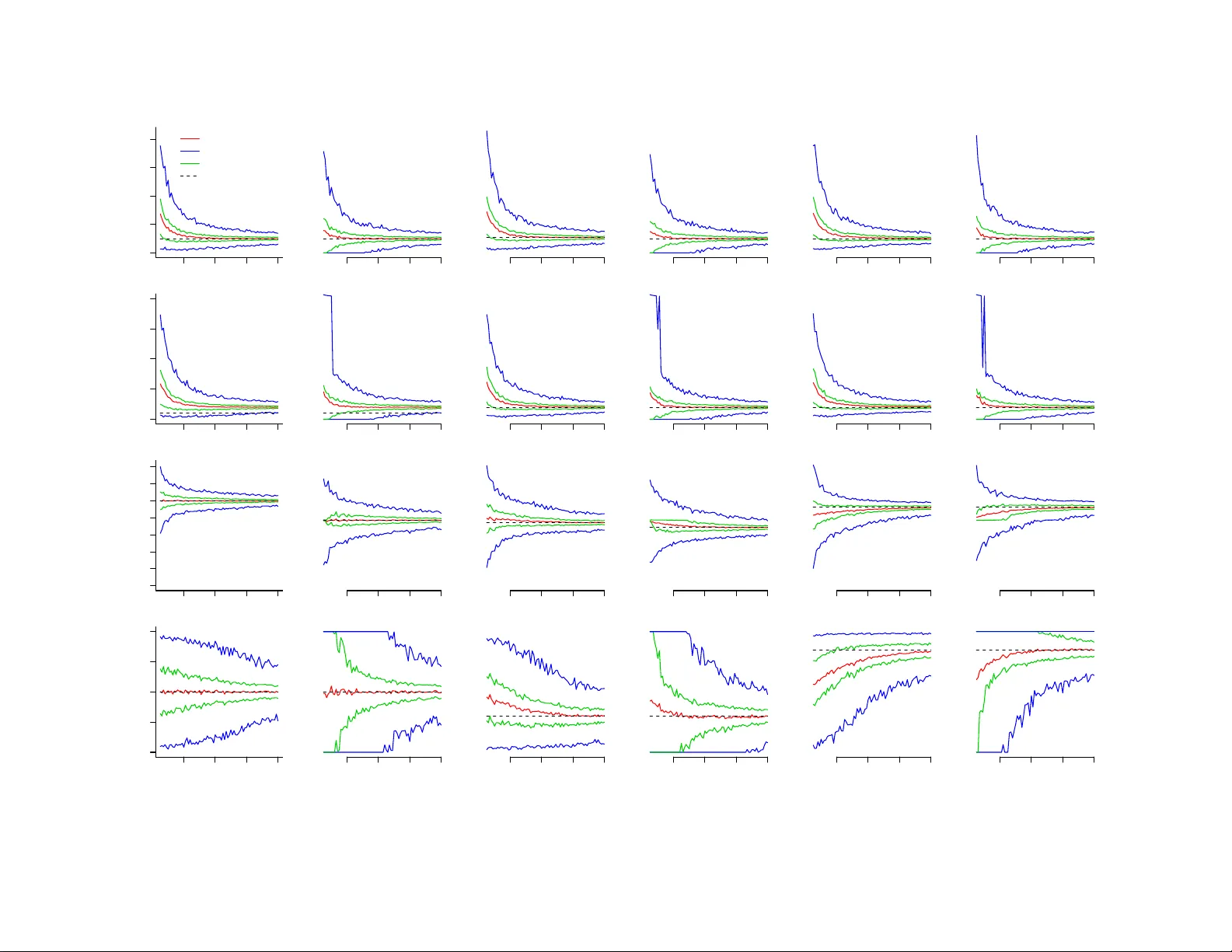
Statistical Prop erties of Sanitized Results from Differen tially Priv ate Laplace Mec hanism with Univ ariate Bounding Constrain ts F ang Liu ∗ Departmen t of Applied and Computational Mathematics and Statistics Univ ersity of Notre Dame, Notre Dame, IN 46556 Abstract Protection of individual priv acy is a common concern when releasing and sharing data and information. Differen tial priv acy (DP) formalizes priv acy in probabilistic terms without making assumptions ab out the background knowledge of data intruders, and th us provides a robust concept for priv acy protection. Practical applications of DP in volv e developmen t of differentially priv ate mechanisms to generate sanitized results at a pre-sp ecified priv acy budget. F or the sanitization of statistics with publicly kno wn b ounds such as prop ortions and correlation co efficien ts, the b ounding constrain ts will need to b e incorp orated in the differen tially priv ate mechanisms. There has b een little w ork on examining the consequences of the b ounding constrain ts on the accuracy of sanitized results and the statistical inferences of the p opulation parameters based on the sanitized results. In this pap er, we formalize the differentially priv ate truncated and boundary inflated truncated (BIT) pro cedures for releasing statistics with publicly kno wn b ounding constrain ts. The impacts of the truncated and BIT Laplace pro ce- dures on the statistical accuracy and v alidit y of sanitized statistics are ev aluated b oth theoretically and empirically via sim ulation studies. keywor ds : truncated mec hanism, boundary inflated truncated (BIT) mec hanism, bias, consistency , mean squared error; global and data-inv arian t ∗ F ang Liu is As sociate Professor in the Department of Applied and Computational Mathematics and Statistics, Universit y of Notre Dame, Notre Dame, IN 46556 ( ‡ E-mail: fang.liu.131@nd.edu). The work w as supp orted b y the NSF Grants 1546373, 1717417, and the Universit y of Notre Dame F aculty Research Initiation Gran t 1 1 In tro duction Protection of individual priv acy is alwa ys a concern when releasing and sharing information. A data release mechanism aims to provide useful information to the public without com- promising individual priv acy . Differen tial priv acy (DP) is a concept developed in theoretical computer science ( Dw ork et al. , 2006b ; Dw ork , 2008 , 2011 ) and has gained great p opularit y in recen t y ears in both theoretical researc h and practical applications. DP formalizes priv acy in mathematical terms without making assumptions ab out the background knowledge of data in truders and thus provides a robust concept for priv acy protection. Practical applications of DP inv olv e dev elopment of differentially priv ate mechanisms, also referred to as sanitiz- ers, through whic h original results are pro cessed and con verted to results that do not reveal individual information at a pre-specified priv acy budget. There are general differen tially priv ate mechanisms such as the Laplace mechanism ( Dw ork et al. , 2006b ), the Exp onen tial mec hanism ( McSherry and T alw ar , 2007 ; McSherry , 2009 ), and more recen tly , the staircase mec hanism ( Geng et al. , 2015 ), the generalized Gaussian mechanism ( Liu , 2016 ), and the adaptiv e mechanisms such as the m ultiplicative weigh ting mechanism ( Hardt et al. , 2012 ) and the median mec hanism ( Roth and Roughgarden , 2010 ) for sanitizing multiple correlated queries. There are also differen tially priv ate mechanisms targeting sp ecifically at certain statistical analyses such as robust and efficien t p oin t estimators ( Dwork and Smith , 2010 ; Dw ork , 2011 ), principle comp onen t analysis ( Chaudh uri et al. , 2012 ), linear and p enalized regression ( Chaudhuri et al. , 2011 ; Kifer et al. , 2012 ), Bay esian inferences of probabilistic graphical mo dels ( Zhang et al. , 2015 ), machine learning, data mining, and big data analytics in genomics, healthcare, biometrics ( Blum et al. , 2008 ; Mohammed et al. , 2011 ; Y u et al. , 2014 ; Lin et al. , 2016 ; Sadhy a and Singh , 2016 ), among others. In the con text of DP , it is sometimes assumed that data and statistics (n umerical query results) are b ounded. The b ounding assumption is supp orted from a tec hnical p ersp ectiv e as well as justified from a practical point of view. First, some statistics are naturally b ounded p er definition, suc h as prop ortions (b ounded b y [0 , 1]) and correlation co efficien ts (b ounded b y [ − 1 , 1]). Second, some statistics are required b e b ounded in order to be sanitized by some of the common differen tially priv ate mec hanisms while ensuring some degree of usefulness of the sanitized results. F or example, the scale parameter of the Laplace mec hanism is prop ortional to the global sensitivit y of a statistic. Suppose the statistic is the sample mean of a n umerical attribute; then the v alue of the attribute needs to b e b ounded on b oth ends to hav e a finite global sensitivit y for the mean so that it can b e sanitized by the Laplace mec hanism in a meaningful w a y . Third, real-life data in general supp ort the assumption of bounded data when the assumption is needed. Though b ounded n umerical attributes in statistical parametric mo delling are often mo delled via distributions with un b ounded domains (e.g., Gaussian or Poisson assumptions), those distributional assumptions are in man y cases only appro ximate and the probabilities of out-of-b ounds v alues are often small enough to b e ignorable under these distributional assumptions. F or instance, it is safe to sa y human heigh t is b ounded within (0 , 300)cm. Though it is often mo delled by Gaussian distributions with support [ −∞ , ∞ ], Pr(heigh t < 0 cm or > 300 cm) ≈ 0 under the Gaussian assumption. If all numerical attributes in a data set are b ounded, descriptive or inferential statistics based on the data in general are also b ounded. F or example, if a n umerical attribute 2 is b ounded within [ c 0 , c 1 ], then its sample mean is b ounded within [ c 0 , c 1 ], and its v ariance is b ounded within [0 , n ( c 1 − c 0 ) 2 / (4( n − 1))] for a given sample size n ( Shiffler and Harsha , 1980 ). Besides the ab o ve examples on the univ ariate b ounding constraint p er statistic, there are also many types of m ultiv ariable b ounding constrain ts. F or example, a linear com bination of m ultiple statistics is b ounded or the sum of a prop ortion v ector is 1. In the follo wing discussion, w e fo cus our theoretical and empirical analysis on the univ ariate b ounding and discuss a couple examples of multiv ariable constraints briefly; more in-depth in vestigation on the latter topic will b e conducted in the future. Mo difications are often needed in some commonly used differen tially priv ate mec hanisms in order to accommo date the release of b ounded statistics without compromising the pre- sp ecified DP . F or example, b oth the Laplace and Gaussian mec hanisms release sanitized re- sults from the real line ( −∞ , ∞ ) and do not automatically deal with b ounding constrain ts. Some practitioners choose to ignore the b ounds and release the raw sanitized results as is. W e would not recommend this approac h since the out-of-b ounds v alues carry no practical meaning and ev entually will b e discarded by data users. Another approach is to form ulate the problem as a constrained optimization problem with inequalit y constraints in the gen- eral framework of constrained inference in DP . The constrained inference approach concerns ab out finding a set of sanitized results that are optimal estimators of the unconstrained sanitized results by some criteria, such as the l 2 distance, sub ject to a set of predefined and known constrain ts. Therefore, “inferences” in this context is not the same as the clas- sical statistical inferences, whic h is ab out inferring p opulation parameters via p oin t and in terv al estimations and hypothesis testing given finite sample data. The constrained in- ference can deal with b oth inequality and equality constraints. F or instance, prop ortions p = ( p 1 , . . . , p K ) T are sub ject to b oth the equality constrain t P K j =1 p j = 1 and the inequality constrain t p j ∈ [0 , 1] for j = 1 , . . . , K . Barak et al. ( 2007 ) emplo yed linear programming (and the F ourier transformation) to obtain a non-negative and consisten t sanitized contin- gency tables. Hay et al. ( 2010 ) b o osted the accuracy of sanitized histograms (measured b y the mean squared error b et ween the sanitized and original results) by incorp orating the prior rank constrain t in unattributed histograms and the equality constrained in universal histograms to increase the accuracy of low er-order marginals. Qarda ji et al. ( 2013 ) sho wed that com bining the choice of a go od branching factor with constrained inference can further b oost the accuracy of a sanitized histogram. Li et al. ( 2015 ) inv estigated an extension to the matrix mechanism they prop osed that incorp orates non-negativity constrain ts when realiz- ing coun t queries. While the constrained inference approach provides a general framework to deal with constraints in DP , all the ab o v e mentioned w ork deals with count data. In addition, the approac h can b e analytically and computationally demanding, dep ending on the statistics and the ob jective functions employ ed. W e will sa ve the in-depth inv estigation of this approac h as a future research topic. In this pap er, we fo cus on examining tw o straightforw ard metho ds that app eal to practi- tioners for sanitizing statistics with b ounding constrain ts. One approach, referred to as the trunc ation pro cedure, throws the out-of-b ounds sanitized v alues aw a y and re-sanitizes until a within-b ound v alue is obtained. This pro cedure can also b e realized by sampling sani- tized results directly from a truncated distribution that satisfies DP . The other approac h legitimizes the out-of-b ounds sanitized results by setting the out-of-b ounds v alues at the 3 b oundaries, referred as the b oundary inflate d trunc ation/BIT pro cedure. This pro cedure can also b e realized by sampling sanitized results directly from a piece-wise distribution with probability mass at the b oundaries. W e assess their impact on the statistical accuracy of sanitized results vs the original results b oth theoretically and empirically in the context of the Laplace mec hanism. T o the b est of our kno wledge, this is the first work on the statistical prop erties of the BIT and truncation b ounding pro cedures in the con text of DP . The rest of the pap er is organized as follo ws. Section 2 ov erviews some of the key concepts in DP . Section 3 presents the truncation and BIT b ounding pro cedures and inv estigates the impact of the BIT and truncation b ounding pro cedures on the utilit y of sanitized results in terms of bias, mean squared error, and consistency . Section 4 illustrates the applications of the truncated and BIT Laplace pro cedures and examines the statistical prop erties of the sanitized results in tw o simulation studies. The pap er concludes in Section 5 with some final remarks and plans for future works. 2 Preliminaries 2.1 Definition of Differen tial Priv acy Let ∆( x , x 0 ) = 1 denote that data x 0 differs from x by only one individual. There are tw o definitions on “differing by one”. Briefly , one refers to the case that the x 0 and x hav e the same sample size n , but one and only one record differs in at least one attributes (a substitution would make the tw o data sets identical). In the second definition, x 0 has one less record that x , so the sample sizes for x is n and n − 1 for x 0 ) (a deletion or a insertion w ould mak e the tw o data sets identical)  -differen tial priv acy (DP) is defined as follows. Definition 1 (  -Differential priv acy ( Dw ork et al. , 2006b )) . A r andomize d me chanism R satisfies  -differ ential privacy if for al l al l data sets ( x , x 0 ) that is ∆( x , x 0 ) = 1 and al l r esult subsets Q to query q ,    log  Pr( R ( q ( x ))) ∈ Q ) Pr( R ( q ( x 0 )) ∈ Q )     ≤  , wher e  > 0 is the privacy budget p ar ameter. Under DP , the ratio in the probabilities of obtaining the same query results from x and x 0 after sanitization via R is b ounded within ( e −  , e  ) – a neighborho o d around 1. F or a small  v alue, the ratio is close to 1, meaning that the query result is similar with or without that individual in the data set, and the chance that a participan t in the data will b e iden tified based on the query result sanitized via R would b e low. DP provides a robust and p o werful mo del against priv acy attacks in the sense that it do es not mak e assumptions on the bac kground knowledge or the b eha vior on data in truders.  can b e used as a tuning parameter – the smaller  is, the more protection there is on the released information via R . There also exist softer v ersions to the pure  -DP that include the ( , δ )-approximate differen- tial priv acy (aDP) ( Dwork et al. , 2006a ), the ( , δ )-probabilistic DP (pDP) ( Mac hanav a jjhala et al. , 2008 ), the ( , δ ) random differen tial priv acy (rDP) ( Hall et al. , 2012 ), and the ( , τ )- concen trated differential priv acy (cDP) ( Dw ork and Roth blum , 2016 ). In all the relaxed v ersions, one additional parameter is emplo yed to characterize the amount of relaxation on top of the priv acy budget  . In ( , δ )-aDP , Pr( R ( q ( x )) ∈ Q ) ≤ e  Pr( R ( q ( x )) ∈ Q ) + δ . A sanitization algorithm satisfies ( , δ )-probabilistic differential priv acy (pDP) if the prob- 4 abilit y of generating an output b elonging to the disclosure set is b ounded b elo w δ , where the disclosure set contains all the p ossible outputs that leak information for a given priv acy tolerance  . The ( , δ )-rDP is also a probabilistic relaxation of DP; but it differs from ( , δ )- pDP in that the probabilistic relaxation is with resp ect to the generation of the data while it is with resp ect to the sanitizer in the ( , δ )-pDP . The ( , τ )-cDP , similar to the ( , δ )-pDP , relaxes the satisfaction of DP with resp ect to the sanitizer, and ensures that the exp ected priv acy cost is  and (Prob(the actual cost >  ) > a ) is b ounded b y e − ( a/τ ) 2 / 2 . 2.2 Laplace Mec hanism and Global Sensitivit y The Laplace mechanism is a p opular sanitizer to release statistics with  -DP ( Dwork et al. , 2006b ). Liu ( 2016 ) in tro duces the generalized Gaussian mec hanism ( , δ )-pDP that includes the Laplace mec hanism as a sp ecial case (when p = 1 and δ = 0). Denote the statistics of in terest by s r × 1 . The Laplace and the generalized Gaussian mechanisms are based on the l p global sensitivity , which is defined as δ p = max x , x 0 ∆( x , x 0 )=1 k s ( x ) − s ( x 0 ) k p = max x , x 0 ∆( x , x 0 )=1 ( P r j =1 | s j ( x ) − s j ( x 0 ) | p ) 1 /p (1) for all pairs of data sets ( x , x 0 ) that are ∆( x , x 0 ) = 1. δ p is the maximum difference in s in the l p distance b et ween any pair of data sets x , x 0 with ∆( x , x 0 ) = 1. The sensitivit y is “global” since it is defined for all p ossible data sets and all p ossible wa ys of tw o data sets differing by one record. The larger the global sensitivit y for s , the larger the disclosure risk is from releasing the original s , and the more p erturbation is needed for s to offset the risk. Sp ecifically , the Laplace mechanism of  -DP sanitizes s r × 1 as in s ∗ r × 1 = ( s 1 , . . . , s r ) ∼ Q r j =1 Lap ( s j , δ 1  − 1 ) , (2) where δ 1 = P r j =1 δ j 1 is the l 1 -global sensitivit y of s and δ j 1 is the glo bal sensitivity of the j -th statistic in s . F or in teger p ≥ 2, the generalized Gaussian mechanism of order p sanitizes s with ( , δ )-pDP b y dra wing sanitized s ∗ from the generalized Gaussian distribution f ( s ∗ ) = Q r j =1 p 2 b Γ( p − 1 ) exp { ( | s ∗ j − s j | /b ) p } = Q r j =1 GG( s j , b, p ) , (3) where b satisfies Pr  P r k =1 a j > b p − δ p p  < δ with a j = P p − 1 j =1 ( p j ) | s ∗ j − s j | p − i δ j 1 ,k , δ 1 ,k = the l 1 - global sensitivit y of s j , and δ p = the l p -global sensitivit y of s . When p = 2, the generalized Gaussian mechanism becomes the Gaussian mec hanism of ( , δ )-pDP that generates sanitized s ∗ j from N( s j , σ 2 = b 2 / 2) for k = 1 , . . . , r . The Laplace and generalized Gaussian mec hanisms pro duce unbound sanitized results from the real line ( −∞ , ∞ ); therefore, some b ounding pro cedures will b e needed if the mechanisms are to b e applied to sanitize b ounded statistics. The global sensitivit y for a query or statistics in general needs to b e determined analytically though its v alue migh t not b e tight. Numerical computation of global sensitivity is not feasible as it is imp ossible to en umerate all p ossible data x and all p ossible w ays of ∆( x , x 0 ) = 1 esp ecially when x contains contin uous attributes or when sample size n is large. W e ha ve obtained the l 1 global sensitivity of some common statistics, including prop ortions, 5 means, v ariances, and co v ariances (refer to the online supplementary materials). The global sensitivit y v alues are calculated for b oth definitions of tw o data sets differing by one record and the global sensitivity is the same on most of the examined statistics regardless of whic h definition is used. F or example, the global sensitivity of the sample mean of a v ariable the v alue of whic h is b ounded within [ c 0 , c 1 ] is n − 1 ( c 1 − c 0 ), and that of the sample v ariance is n − 1 ( c 1 − c 0 ) 2 . In all calculations, we assume the sample size n of the original data is a known and carries no priv acy concern, whic h is often the case in statistical analysis. It should b e noted that the global sensitivity of a function of a statistic s is not equal to the function of the global sensitivit y of s in general. F or example, δ 1 of a sample v ariance is ( c 1 − c 0 ) 2 n − 1 , but δ 1 of the sample standard deviation cannot b e simply calculated as p ( c 1 − c 0 ) 2 n − 1 . In fact, the global sensitivity of the standard deviation is more difficult to calculate analytically compared to that of the v ariance. When the global sensitivity of s is not easy to calculate, but a data-indep enden t function of s , say t = f ( s ), is, we can instead sanitize t to obtain t ∗ and then obtain sanitized s ∗ via the bac k-transformation s ∗ = f − 1 ( t ∗ ). 3 T runcated and BIT Laplace Mec hanisms In this section, we first formalize t w o commonly used b ounding pro cedures and then examine the statistical properties of sanitized outcomes processed b y the t wp pro cedures, respectively . Both pro cedures are in tuitiv e and straightforw ard to apply and can b e coupled with any dif- feren tially priv ate mechanisms. W e fo cus on their applications in the context of the Laplace mec hanism giv en its p opularit y , and will lo ok into their applications in other mec hanisms as the generalized Gaussian mechanism in the future. 3.1 Definitions Definition 2 ( truncated and b oundary-inflated-truncated Laplace mechanisms ) . Denote the b ounde d statistics by s r × 1 = ( s 1 , . . . , s r ) ∈ [ c 10 , c 11 ] × · · · × [ c r 0 , c r 1 ] , wher e [ c j 0 , c j 1 ] ar e the b ounds for i th element in s ( i = 1 , . . . , r ), the privacy budget by  , the l 1 -glob al sensitivity of s by δ 1 . L et λ = δ 1  − 1 . (a) The trunc ate d L aplac e me chanism of  -DP sanitizes s by dr awing s ∗ fr om the trun- c ate d L aplac e distribution f ( s ∗ ) = r Y j =1 L ap ( s j , λ | c j 0 ≤ s ∗ ≤ c j 1 ) = r Y i =1 exp  − | s ∗ j − s j | λ  2 λ  1 − 1 2 exp( − c j 1 − s j λ ) − 1 2 exp( c j 0 − s j λ )  . (4) (b) The b oundary-inflate d-trunc ate d (BIT) L aplac e me chanism of  -DP sanitizes s by dr awing s ∗ fr om the BIT L aplac e distribution f ( s ∗ ) = Q r i =1 f ( s ∗ j ) , wher e f ( s ∗ j ) is f ( s ∗ j ) =      1 2 exp( − ( s j − c j 0 ) /λ ) if s ∗ j = c j 0 L ap ( s j , λ ) if c j 0 < s ∗ j < c j 1 1 − 1 2 exp( − ( c j 1 − s j ) /λ ) if s ∗ j = c j 1 (5) 6 Rather than sampling directly from Eqn ( 4 ), the truncated Laplace mec hanism can also b e realized via in a p ost-ho c manner by thro wing aw a y out-of-b ounds sanitized results from the regular Laplace mec hanism until catc hing an in-b ound v alue. Similarly , the BIT b ounding pro cedure can b e realized b y p ost-ho c setting out-of-b ounds sanitized results from the regular Laplace mechanism at the corresp onding b oundaries. If the scale parameter λ → ∞ in the Laplace distribution when  → 0 or δ 1 → ∞ , it can b e easily established that f ( s j ) in the truncated Laplace mechanism in Eq. ( 4 ) conv erges to an uniform distribution unif( c 0 i , c 1 i ), and that in the BIT Laplace distribution in Eq. ( 5 ) con v erges to a Bernoulli distribution with probabilit y mass at c 0 i and c 1 i , resp ectively . In b oth of the asymptotic cases, the sanitized results preserve little original information. Both the Laplace and BIT Laplace mec hanisms, as in the regular Laplace mechanism, require calculation of the l 1 -global sensitivity for the targeted s to b e sanitized. Remark 1 ( multiv ariable-function constrain ts ) . Definition 2 fo cuses on the c ase wher e e ach statistic s j in s has its own lower and upp er b ounds [ c 0 j , c 1 j ] ( j = 1 , . . . , r ) that ar e publicly known and fixe d c onstants. In some pr actic al c ases, b esides the b ounding c onstr aints for e ach statistic, a subset of s or al l of its elements ar e also r e quir e d to satisfy multivariable c onstr aints. F or example, s is a set of pr op ortions under the line ar c onstr aint P r j =1 s j = 1 ; or a subset S of s satisfies c 0 ≤ P k ∈S a k s k ≤ c 1 . In the pr esenc e of the additional multivariable c onstr aints, one would first che ck whether the multivariable c onstr aints ar e c omp atible with the b ounding c onstr aint on e ach s j , which may le ad to a set of new c onstr aints that inc orp or ate al l the c onstr aints – univariate or multivariate. F or example, say s = ( s 1 , s 2 ) and the line ar c onstr aint is s 1 + s 2 = c . The final c onstr aints on s 1 and s 2 would then b e [max( c − c 12 , c 01 ) , min( c − c 02 , c 11 )] and [max( c − c 11 , c 02 ) , min( c − c 01 , c 12 )] , r esp e ctively. After applying either the trunc ate d or the BIT L aplac e me chanism in Definition 2 to sanitize, say s 1 to obtain s ∗ 1 , that satisfies the new b ounding c onstr aint, the other c an b e c alculate d as s ∗ 2 = c − s ∗ 1 . In some sp e cial c ases, such as when s is a set of pr op ortions under the line ar c onstr aint P r j =1 s j = 1 , one c an also apply a simple r esc aling pr o c e dur e to the sanitize d s to satisfy the multivariable line ar c onstr aint (se e simulation study 2 in Se ction 4 for an example). There are many t yp es of m ultiv ariable constrain ts. Dep ending on the nature of the additional m ultiv ariable constraints, there ma y exist different approaches to satisfy all the constrain ts sim ultaneously – some might lead to b etter original information preserv ation than others for the same priv acy budget. In addition, the computational complexity to obtain a set of sanitized s ∗ that satisfy all the constrain ts may reach a lev el b eyond practicalit y . The diver- sit y and complexity of satisfying m ultiv ariable constrain ts also indicates c hallenges for the theoretical analysis on the statistical prop erties of sanitized s ∗ in this setting. F or these rea- sons, in the theoretical analysis in Section 3.2 , w e fo cus on learning the statistical prop erties of sanitized s ∗ where each of its elemen t has only the univ ariate b ounding constraint with no additional m ultiv ariable constrain ts. Incorp orating m ultiv ariable-function constrain ts on top of the univ ariate b ounding constraints deserv es more in-depth inv estigation and will b e a topic of future researc h. 7 3.2 Statistical Prop erties of Sanitized s ∗ under Univ ariate Bound- ing Constrain t In Definition 2 , the b ounds [ c 10 , c 11 ] × · · · [ c r 0 , c r 1 ] are assumed to b e data inv arian t and “global” to guaran tee  -DP , from the data release p ersp ectiv e. If the b ounds are “lo cal” and data-sp ecific, meaning they are functions of data x at hand, then the b ounds themselv es, w ould need to b e sanitized and would otherwise leak information ab out the original data. On the other hand, ignoring the lo cal prop erties of data x in a b ounding pro cedure could ha ve a negative impact on the statistical prop erties of sanitized results s ∗ . In this section, we in vestigate the statistical behaviors of s ∗ pro duced by a sanitizer with b ounding constraints. The rationale for studying the statistical prop erties of the sanitized statics is as follows. First, duo to randomness of the injected noise to satisfy DP , the sanitized statistic is a random v ariable (even without accoun ting for the sampling v ariabilit y of the sample data after conditional on the original static). Though the priv acy budget is often only enough for querying one or a few statistics, the users would still b e interested in understanding and gaining theoretical insights on the statistical prop erties of the sanitized statistic in exp ectation o v er the distribution of the injected noise, such as bias and MSE of the sanitized statistic. F urthermore, one of the main goals for data collection is to draw inferences ab out the p opulation from whic h the sample data come from. F or non-priv ate inferences, one would often examine the statistical prop erties of an estimator given sample data to see how go od it is for a p opulation parameter, suc h as un biasedness and consistency . In the con text of priv ate inferences, the users w on’t hav e access to the original non-priv ate estimate, but rather its sanitized v ersion. If the sanitized statistic do es not p ossess desirable statistical prop erties, sa y it is biased, for the original statistic, and even if the original statistic is un biased for the p opulation parameter, then users know the statistical inference based on the sanitized statistic would b e biased as w ell, p er the la w of total exp ectation. W e start b y defining the desired statistical prop erties of sanitized s ∗ (Definition 3 ), then examine the bias of s ∗ sanitized by the truncated and BIT Laplace mechanisms relativ e to the original s (Prop osition 1 ), and present an upp er b ound for the mean squared error and examine the consistency of s ∗ for s and the conv ergence rate in Prop osition 2 . In addition, w e list in Prop osition 3 a set of sufficient conditions for the sanitized s ∗ to b e asymptotically un biased and consistent for the p opulation parameter θ in the case where the original s is an estimator for θ . Definition 3 ( un biasedness and consistency of sanitized statistic for original statis- tic ) . Sanitize d s ∗ is unbiase d for the original s if E s ∗ ( s ∗ | s ) = s ; s ∗ is asymptotic al ly unbiase d for s if E s ∗ ( s ∗ | s ) → s as n → ∞ , wher e n is the sample size of original data x ; s ∗ is c onsistent for s if s ∗ p − → s as n → ∞ . When s is b oundless and sanitized by the regular Laplace mec hanism, then s ∗ is unbiased for s since E( s ∗ ) = s p er the definition of the Laplace distribution. If δ 1 ∝ n − k , where k > 0, then s ∗ is also consistent for s . When s is b ounded and sanitized via the truncated or BIT Laplace mechanism, we will ha ve biased s ∗ unless the b ounds are symmetric around the original s . Prop osition 1 states the formal conclusions and presen ts the magnitude of 8 the bias of s ∗ in the truncated and BIT Laplace mechanisms. The pro of of Prop osition 1 is pro vided in App endix A . Prop osition 1 ( bias of sanitized statistic from truncated and BIT Laplace mec h- anisms ) . L et [ c 0 , c 1 ] b e the glob al b ounds on a singular s , λ b e the sc ale p ar ameter, s b e the lo c ation p ar ameter of the L aplac e distribution, µ 1 b e the exp e cte d me an of the trunc ate d L aplac e distribution f ( s ∗ | s ∗ ∈ [ c 0 , c 1 ]) , and µ 2 b e the exp e cte d me an of the BIT L aplac e dis- tribution define d in Eqn ( 5 ). Then µ 1 = s + λ − c 0 + s 2 exp  c 0 − s λ  − λ + c 1 − s 2 exp  s − c 1 λ  1 − 1 2 exp( c 0 − s λ ) − 1 2 exp( s − c 1 λ ) (6) µ 2 = s + λ 2  exp  c 0 − s λ  − exp  s − c 1 λ  (7) (a) µ 1 = µ 2 = s ( s ∗ is unbiase d for s ) if and only if c 0 + c 1 = 2 s ( c 0 and c 1 ar e symmetric ar ound s ). (b) ( µ 1 − s )( µ 2 − s ) ≥ 0 (the dir e ction of the bias is the same b etwe en the two). Sp e cific al ly, µ 1 − s ≥ 0 and µ 2 − s ≥ 0 if s − c 0 < c 1 − s ; µ 1 − s ≤ 0 and µ 2 − s ≤ 0 if s − c 0 > c 1 − s . (c) | µ 1 − s | ≥ | µ 2 − s | ( s ∗ sanitize d via the BIT L aplac e sanitizer is no mor e biase d than that via the trunc ate d L aplac e sanitizer). F or the global and data in v arian t b ounds [ c 0 , c 1 ], it is unlikely the sanitized results would b e un biased via the truncated or the BIT Laplace mechanism p er part (a) of Prop osition 1 as [ c 0 , c 1 ] are fixed while the original statistic s c hanges from data to data. T o ac hiev e un biasedness for s ∗ , lo cal b ounds that dep end on sp ecific data sets can b e constructed at additional priv acy cost. F or example, b ounds [ s − min( s − c 0 , c 1 − s ) , s + min( s − c 0 , c 1 − s )], whic h are symmetric around s , can b e used to b ound sanitized results in the truncated and BIT Laplace mec hanism that leads to unbiased s ∗ . Ho wev er, since the b ounds are functions of the original s , they will leak information ab out s , whic h has to b e counted for in the total priv acy cost. Remark 2 ( Extension of Prop osition 1 to m ultidimensional s ) . Pr op osition 1 exam- ines a sc alar query s . The c onclusions c an b e e asily extende d to s r = ( s 1 , . . . , s r ) of arbitr ary dimension r ≥ 1 with univariale b ounding c onstr aint p er statistic. The only differ enc e lies in how the sc ale p ar ameters λ is define d. As given in Eqn ( 2 ), the L aplac e me chanism for sanitizing s r × 1 is Q r j =1 L ap ( s j , δ 1  − 1 ) with δ 1 = P r j =1 δ j 1 , wher e δ j 1 is the glob al sensitivity of s j , the j -th statistic in s . We c an r ewrite The joint distribution of sanitize d s ∗ as r Y j =1 L ap s j , δ 1 j   δ 1 j δ 1  − 1 ! = r Y j =1 L ap ( s j , δ 1 j ( w j  ) − 1 ) , wher e w j = δ 1 j /δ (8) In other wor ds, the L aplac e me chanism c an b e r e gar de d as a sp e cial applic ation of the se- quential c omp osition ( McSherry , 2009 ) by al lo c ating a p ortion w j = δ 1 j /δ of total  to the sanitization of s j (also r efer to Liu ( 2017 )). F or the sc enario examine d in this p ap er, that is, the b ounds for s ar e publicly known and fixe d, the c onclusions fr om Pr op osition 1 apply 9 to e ach element s j in s r × 1 with differ ent b ounds [ c 0 j , c 1 j ] and sc ale p ar ameter λ j = δ j ( w j  ) − 1 for differ ent s j in Eqns ( 6 ) and ( 7 ). Remark 3 ( Prop osition 1 for one-sided b ounding constrain ts ) . The c onclusions in Pr op osition 1 ar e also applic able in the sp e cial c ases when the b ounds ar e one-side d [ c 0 , ∞ ] or [ ∞ , c 1 ] , if such ne e ds exist in pr actic e. The pr o of and establishment of these c onclusions do not imp ose any r estrictions on the values c 0 and c 1 exc ept for the trivial r e quir ement c 0 < c 1 . The bias terms actual ly have simpler expr ession in the c ase. Sp e cific al ly, Eqns ( 6 ) and ( 7 ) b e c ome b ounds [ c 0 , ∞ ) : µ 1 = s + λ − c 0 + s 2 exp  c 0 − s λ  1 − 1 2 exp( c 0 − s λ ) ; µ 2 = s + λ 2 exp  c 0 − s λ  (9) b ounds ( −∞ , c 1 ] : µ 1 = s − λ + c 1 − s 2 exp  s − c 1 λ  1 − 1 2 exp( s − c 1 λ ) ; µ 2 = s − λ 2 exp  s − c 1 λ  . (10) It is e asier (c omp ar e d to the gener al c ase of [ c 0 , c 1 ] ) to se e that b oth biases fr om the trun- c ation and the BIT pr o c e dur es ar e p ositive when the b ounds ar e [ c 0 , ∞ ) , a sp e cial c ase of s − c 0 < c 1 − s in p art b), and ne gative when the b ounds ar e ( −∞ , c 1 ] a sp e cial c ase of s − c 0 > c 1 − s . The differ enc e of the two bias terms when the b ounds ar e [ c 0 , ∞ ] is  1 − ( c 0 − s ) /λ 1 − exp( c 0 − s λ ) / 2 − 1  λ 2 exp  c 0 − s λ  . Sinc e 0 < 1 − exp( c 0 − s λ ) / 2 < 1 / 2 and 1 − ( c 0 − s ) /λ > 1 , thus the bias differ enc e is > 0 . Sinc e b oth biases ar e p ositive, this implies that µ 1 has a lar ger p ositive bias than µ 2 . Similarly, when the b ounds ar e [ −∞ , c 1 ] , the bias differ enc e b etwe en µ 1 and µ 2 is  1 − 1+( c 1 − s ) /λ 1 − exp( s − c 1 λ ) / 2  λ 2 exp  s − c 1 λ  . Sinc e 0 < 1 − exp( c 1 − s λ ) / 2 < 1 / 2 , and 1 + ( c 1 − s ) /λ > 1 , the bias differ enc e is < 0 . Sinc e b oth biases ar e ne gative, this implies that µ 1 has a lar ger ne gative bias than µ 2 . T aken to gether, | µ 1 − s | > | µ 2 − s | . In addition to quan tify the magnitude of bias, it is also of interest to b ound the error of a sanitized statistic relative to its original v alue. Prop osition 2 examines the upp er b ound for the mean squared error (MSE) for a sanitized statistic via the truncated and BIT Laplace mec hanisms, and establishes the condition under whic h the statistic would be MSE-consistent for its original v alue, and the conv ergence rate of consistency . Prop osition 2 ( consistency and con v ergence rate ) . L et s b e the lo c ation p ar ameter and λ b e the sc ale p ar ameter of the L aplac e distribution, and s ∗ b e the sanitize d r esult for s via the trunc ate d or the BIT L aplac e me chanism. The MSE E s ∗ ( s ∗ − s ) 2 is upp er b ounde d by 2 λ 2 = 2( δ 1 / ) 2 and s ∗ is MSE-c onsistent for s as λ → 0 . If δ 1 ∝ n − k , wher e k > 0 and n is the sample size, then the r ate of the MSE c onver ging to 0 is O ( n − 2 k ) for a given  . The pro of is provided in App endix B . The pro of do es not hav e restrictions on the v alues of c 0 or c 1 , which can b e as extreme as c 1 = ∞ and c 0 = −∞ . Therefore, the conclusions in Prop osition 2 also to the non-sided b ounding constraints. In addition, similar to Remark 2 for Prop osition 1 , the established conclusions in Prop osition 2 can b e easily extended to s r = ( s 1 , . . . , s r ) of arbitrary dimension r ≥ 1 with univ ariate b ounding constrain t. The only 10 difference is that the statistic-sp ecific λ j ( j = 1 , . . . , r would b e used. Therefore, differen t elemen ts from s r will hav e different MSE b ounds and differen t con vergence rates. Prop osition 2 sho ws that the sanitized result, though lik ely biased p er Proposition 1 , can still enjo y nice asymptotic prop erties suc h as asymptotic un biasedness and consistency as λ → 0 . In the framew ork of the truncated and BIT Laplace mechanisms, the scale parameter of the asso ciated Laplace distribution λ is δ 1  − 1 . F or a pre-sp ecified  , to satisfy the condition λ → 0, then δ 1 needs to b e → 0. In tuitively speaking, as n increases, the influence of a single individual on an aggregate measure of a data set is lik ely to diminish, and the individual is less prone to b e identified from releasing the aggregate measure. T ranslated to the global sensitivit y of the aggregate measure, it means that δ 1 decreases with n . δ 1 of some commonly used statistics are ∝ n − 1 , such as prop ortions, means, v ariances and co v ariances (refer to the online supplemental materials), and the sanitized copies of these statistics via either the truncated or BIT Laplace mec hanism are consisten t for their original v alues by part c) of Prop osition 1 . The results in Prop osition 2 imply that the MSE of a sanitized statistic from the truncated or the BIT Laplace mechanism is comparable to the MSE from the regular Laplace mechanism without b ounding, which is also 2 λ 2 . In other words, the b ounding do es not seem to affect the MSE of a sanitized statistic despite the loss of un biasedness in general. Prop ositions 1 and 2 examine the statistical prop erties of the sanitized s ∗ relativ e to the original s . In many statistical analysis, the ultimate goal is to infer unknown p opulation parameters θ based on the sample data. Supp ose s is an estimator for parameter θ in a statistical mo del. Prop osition 3 lists the sufficient conditions for s ∗ , the sanitized version of s , to b e asymptotically unbiased and consistent for θ . Prop osition 3 ( asymptotic un biasedness and consistency of sanitized statistic for p opulation parameter ) . . (a) If E ( s | θ ) = θ or E ( s | θ ) → θ , and if E s ∗ ( s ∗ | s ) → s as n → ∞ , then s ∗ is asymptotic al ly unbiase d for θ ; that is, E ( s ∗ | θ ) → θ . (b) If s ∗ p − → s and s p − → θ as n → ∞ , then s ∗ is c onsistent for θ ; that is, s ∗ p − → θ . The pro of of Proposition 3 is given in App endix C . Note that Prop osition 3 does not list the conditions for obtaining an un biasedness s ∗ for θ as it is meaningless given the lo w likelihoo d of obtaining an un biased s ∗ for s p er Prop osition 1 . Prop osition 3 implies that asymptotic un biasedness and consistency of the sanitized s ∗ for θ can b e achiev ed in tw o steps. In step one, we will c ho ose an estimator s that is asymptotically unbiased or consistent for θ , which should b e relativ ely straigh tforward giv en that these t yp es of estimators are w ell studied and widely applied in statistics; in the second step, w e will employ an appropriate differentially priv ate mechanism to generate s ∗ that is asymptotically unbiased or consistent for s , such as the BIT and truncated Laplace mechanisms, whic h yield MSE-consistent s ∗ for s under the conditions listed in Prop ositions 2 . 4 Sim ulation Studies W e conducted tw o simulation studies to demonstrate the applications of the truncated and BIT b ounding mechanisms and examine the statistical prop erties of the sanitized results. In 11 the first sim ulation, we sanitized a v ariance-co v ariance matrix, and fo cused on the compar- isons b et w een the sanitized results and the original results and b et ween the truncated and BIT truncated Laplace mechanisms on the effects on the sanitized results. In the second sim ulation, w e sanitized prop ortions and fo cused on the inferential prop erties of the san- itized prop ortions by examining the bias, ro ot mean squared error (RMSE) and cov erage probabilit y (CP) for the true prop ortions based on the sanitized results. 4.1 Sim ulation Study 1 In this simulation, w e applied the truncated and BIT Laplace mec hanisms to sanitize a v ariance-cov ariance matrix S in a data set of size n . The v ariance-co v ariance matrix is a widely used statistic for examining the dep endency structure among multiple con tinuous v ariables. It is also an ideal statistic to examine the effects of the t wo mec hanisms given that ev ery element in the matrix has to satisfy some type of b ounding constraints. The b ounding constraints of a cov ariance matrix of an y dimension include that the marginal v ariances are p ositiv e and the correlations are b ounded b etw een [-1, 1]. Additionally , the marginal v ariances are righ t-b ounded in b ounded data from which S is calculated. T able 1 summarizes the b ounds and global sensitivity of the comp onents in S . T able 1: Glob al sensitivity of varianc e and c ovarianc e terms in a c ovarianc e matrix statistic b ounds ‡ δ 1 v ariance S j j (0 , n ( c j 1 − c j 0 ) 2 / (4( n − 1))] ( c j 1 − c j 0 ) 2 /n v ariance S j 0 j 0 (0 , n ( c j 0 1 − c j 0 0 ) 2 / (4( n − 1))] ( c j 0 1 − c j 0 0 ) 2 /n co v ariance S j j 0 ( − p S j j S j 0 j 0 , p S j j S j 0 j 0 ) ( c j 1 − c j 0 )( c j 0 1 − c j 0 0 ) /n ‡ [ c j 0 , c j 1 ] × [ c j 0 0 , c j 0 1 ] w ere the b ounds of v ariables X j and X j 0 When sanitizing S in general, w e first obtain legitimate sanitized S ∗ j j and S ∗ j 0 j 0 , and then sani- tize S j j 0 giv en S ∗ j j and S ∗ j 0 j 0 under the constraint that S ∗ j j 0 ∈ [ − p S ∗ j j S ∗ j 0 j 0 , p S ∗ j j S ∗ j 0 j 0 ]. Though the b ounds for S ∗ j j 0 dep end on S ∗ j j and S ∗ j 0 j 0 , the latter t wo are already sanitized; therefore, b ounding pro cedures for S ∗ j j 0 using information S ∗ j j and S ∗ j 0 j 0 do es not incur additional priv acy cost. The in terv al constrain t on S ∗ j j 0 do es not hav e to contain the original S j j 0 . Comparing to containing S j j 0 , which w ould b e nice from information preserv ation p erspective, satisfying the hardcore requirement that the P earson correlation is within [ − 1 , 1] is necessary , when there is a conflict betw een the tw o. In addition, requiring the interv al to contain the original S j j 0 w ould also lead to priv acy leak, strictly sp eaking. It is p ossible that the sanitized cov ariance matrix S ∗ is not p ositiv e definite (PD) with the elemen t-wise sanitization approac h. If a sanitized co v ariance matrix is not PD and has a significan t num ber of (small) negativ e eigenv alues, it can b e made PD with semi-definite optimization via, e.g., the alternating pro jections algorithm ( Higham , 2002 ), the Newton metho ds for nearest correlation matrix ( Qi and Sun , 2006 ; Borsdorf and Higham , 2010 ), and the spectral pro jected gradien t metho d ( Qi and Sun , 2006 ; Borsdorf et al. , 2010 ) 1 . A possible alternativ e is to sanitize S as a whole instead of element-wise, an interesting and worth while topic for future research. 1 The R function nearPD() in pack age Matrix implemen ts the alternating pro jections algorithm. 12 W e examined in this simulation study a 2 × 2 v ariance-co v ariance matrix with three differen t sp ecifications of ( S 11 , S 22 , r ): (1 , 2 , 0) , (1 , 2 , − 0 . 4), and (1 , 2 , 0 . 7), resp ectively . The 3 correla- tion settings allo w us to examine the b ounding effects on the pairwise correlation when there is no correlation, mo derate (negative) correlation, and strong (p ositiv e) correlation. W e set the global b ounds [ c 10 , c 11 ] at [ − 3 , 3] and [ c 20 , c 21 ] at [ − 4 . 5 , 4 . 5] 2 . The total priv acy budget w as  = 1. Since the 3 statistics w ere calculated on the same set of data, the sequential comp osition principle applied ( McSherry , 2009 ) when it comes to priv acy budgeting. There are different w ays to allo cate the total budget when sanitizing multiple statistics calculated from the same data set, such as by an equal allo cation across all the statistics or according to some type statistical or practical “importance” of the statistics (see Liu ( 2017 ) for more dis- cussion). Here we divided the total priv acy budget  equally among the 3 statistics; that is, eac h sanitization received 1 / 3 of the total budget. W e also inv estigated a wide range of sam- ple size n from 50 to 800. In eac h examined scenarios of ( S , n ), 500 independent sanitizations w ere carried out to examine the distributional prop erties of the sanitized results. The results are presented in Figure 1 . In eac h plot, the av erage and the (2.5%, 25%, 75% and 97.5%) p ercen tiles of the sanitized results from the 500 sanitizations are presen ted, b enc hmark ed against the original results. The main findings are summarized as follo ws. First, when n was relativ ely small, there w as noticea ble bias in the sanitized results compared to the original results, except for S 12 and r when r = 0 (the b oundaries were symmetric ab out the original results and thus there was no bias p er part (a) of Prop osition 1 ). Second, the sanitized results generated via the truncated Laplace mechanism were more biased than those via the BIT Laplace mec hanism, consistent with part (b) of Prop osition 1 . Third, as n increased, b oth the bias and disp ersion of the sanitized results approached 0, consistent with part (c) of Prop osition 1 . Lastly , when n w as small, the scale parameter asso ciated with the Laplace distribution in b oth mechanisms was large, therefore more sanitized v alues w ere set at the b oundary v alues in the BIT mec hanism and the distribution of the sanitized v alues b ecame flatter in the truncated mechanism, esp ecially for r . 2 F or approximately Gaussian v ariables with means 0, b oth the bounds of [ − 3 , 3] with a standard deviation of 1 and [ − 4 . 5 , 4 . 5] with a standard deviation of √ 2 represen t > 99% data mass though this simulation did not require the Gaussian assumption. 13 200 400 600 800 0 2 4 6 8 n apply(S11[, −1], 1, mean) n S11* truncated r = 0 mean (2.5,97.5)% (25,75)% original 200 400 600 800 0 5 10 15 20 n apply(S22[, −1], 1, mean) n S22* 200 400 600 800 −10 −6 −2 0 2 4 n apply(S12[, −1], 1, mean) n S12* 200 400 600 800 −1.0 −0.5 0.0 0.5 1.0 apply(rho[, −1], 1, mean) n r* n apply(S11[, −1], 1, mean) 200 400 600 800 BIT r = 0 n apply(S22[, −1], 1, mean) 200 400 600 800 n apply(S12[, −1], 1, mean) 200 400 600 800 apply(rho[, −1], 1, mean) 200 400 600 800 n apply(S11[, −1], 1, mean) 200 400 600 800 truncated r = −0.4 n apply(S22[, −1], 1, mean) 200 400 600 800 n apply(S12[, −1], 1, mean) 200 400 600 800 apply(rho[, −1], 1, mean) 200 400 600 800 n apply(S11[, −1], 1, mean) 200 400 600 800 BIT r = −0.4 n apply(S22[, −1], 1, mean) 200 400 600 800 n apply(S12[, −1], 1, mean) 200 400 600 800 apply(rho[, −1], 1, mean) 200 400 600 800 n apply(S11[, −1], 1, mean) 200 400 600 800 truncated r = 0.7 n apply(S22[, −1], 1, mean) 200 400 600 800 n apply(S12[, −1], 1, mean) 200 400 600 800 apply(rho[, −1], 1, mean) 200 400 600 800 n apply(S11[, −1], 1, mean) 200 400 600 800 BIT r = 0.7 n apply(S22[, −1], 1, mean) 200 400 600 800 n apply(S12[, −1], 1, mean) 200 400 600 800 apply(rho[, −1], 1, mean) 200 400 600 800 Figur e 1: Sanitize d c omp onents in S ( ( Q 1 , Q 2 ) % r epr esents the Q 1 and Q 2 p er c entiles of the distribution of the sanitize d statistic) 14 4.2 Sim ulation Study 2 In this sim ulation, w e aimed to release a prop ortion vector p where P K j =1 p j = 1. Prop ortions are v ery common statistics in public data release. F or example, p could be the proportions of differen t income lev els in the US p opulation, or the cell prop ortions from a cross-tabulation of, say gender and race. Besides the b ounding constrain t [0 , 1] on eac h prop ortion comp onen t, p is also sub ject to the equality constrain t P j =1 p j = 1, whic h has to b e retained in the released sanitized results, making it an interesting problem to study . Since the prop ortions are calculated from disjoin t subsets of data, the addition or remo v al of a single observ ation affects the coun t in exactly one cell, the global sensitivit y ( δ 1 ) of releasing p is n − 1 or 2 n − 1 , dep ending on which definition of “differing by one record” is used on ∆( x, x 0 ) = 1 (refer to the online supplementary materials). With the Laplace mechanism, sanitization of eac h prop ortion in p is p erturbed with a noise term from Lap( δ 1  − 1 ). In this simulation, w e used δ 1 = n − 1 , and examined 3 differen t sp ecifications of  (0 . 1 , 0 . 5 , 1) and a range of sample size ( n = 50 ∼ 500) (the results obtained from this simulation are also applicable to δ 1 = 2 n − 1 with doubled  ). 500 m ultinomial data sets, eac h sized at n , w ere simulated from m ultinomial( n, p ). W e examined a 4-elemen t p in this simulation and set p = (0 . 1 , 0 . 2 , 0 . 3 , 0 . 4) (these parameter v alues were c hosen b ecause they expand a wide range – some are closer to the b oundaries while others are closer to the center, allowing us to examine the effects of the binding mechanisms on prop ortions of different magnitude). The sample prop ortions ˆ p were calculated in each rep eat and w ere sanitized via the trun- cated and BIT Laplace mechanisms resp ectively . W e employ ed 3 pro cedures to ensure the equalit y constraint P 4 k =1 p k = 1 was met (in addition to the b ounding constrained on each prop ortion). In the first approach (re-scaling and normalization), each proportion in ˆ p j w as sanitized indep enden tly to obtain the p erturb version ˆ q ∗ k , which w as then normalized to ob- tain ˆ p ∗ j = ˆ q ∗ k ( P 4 k =1 ˆ q ∗ k ) − 1 ; it is ˆ p ∗ that w as released. This re-scaling approac h was intuitiv e and straigh tforward. In the second approach, referred to as the all-but-one approach, we sanitized 3 proportions out of 4, and then calculated the 4-th proportion via 1 − P 3 k =1 ˆ q ∗ k . The all-but-one approac h ob ey ed the equalit y constraint during the sanitization without p ost- pro cessing as in the re-scaling approach. In the third approach, referred to as the univ ersal histogram/UH approach, we applied a sligh tly mo dified pro cedure from Hay et al. ( 2010 ) to ensure the equality constraint in p . In the original UH pro cedure in Hay et al. ( 2010 ), the ro ot no de is sanitized and there is no inequality constrain t; in our case, the ro ot no de was fixed at 1 as it w as the summation of p , and there were inequality constraints. Since the UH requires the n umber of c hildren per no de to b e constant across the whole tree and there needs to b e at least three lay ers in the tree (since the ro ot no de is fixed at one in our case) in order to sho w any level of impro vemen t in the accuracy of some of the sanitized no des, the four prop ortions in p , represen ted by four leaf no des, are th us com bined in a binary fashion in 3 la yers; otherwise, it w ould b e the same as the re-scaling approac h. 1. Arrange the 4 prop ortions in a 3-lay er binary tree structure. The ro ot no de in the tree alw ays has a v alue of 1, and its t w o c hild no des h 1 and h 2 in lay er 2 satisfy the constrain t h 1 + h 2 = 1 (equalit y constraint 1). Similarly , the tw o child no des of h 1 ( h 11 and h 12 in la yer 3) satisfy h 11 + h 12 = h 1 (equalit y constraint 2) and the t wo child no des of h 2 ( h 21 15 and h 22 in lay er 3) satisfy h 21 + h 22 = h 2 (equalit y constraint 3). As a result, the four leaf no des in lay er 3, corresp onding to the 4 prop ortions in p , satisfy h 11 + h 12 + h 21 + h 22 = 1. 2. Sanitize h 1 and h 2 in lay er 2, and ( h 11 , h 12 , h 21 , h 22 ) in lay er 3 via the BIT and Laplace Laplace mechanisms with the scale parameter 2 / ( n ). The global sensitivity doubles in this pro cedure as there are tw o sets of prop ortions to b e sanitized on the same data set. 3. Calculate the inconsistent counts z (due to sanitization) for the no des in the tree. Let h ∗ ( v ) = { h ∗ 1 , h ∗ 2 , h ∗ 11 , h ∗ 12 , h ∗ 21 , h ∗ 22 } denote the sanitized results from step 2. z ( v ) = h ∗ ( v ) if v is a leaf no de in lay er 3, and z ( v ) = 1 3 P v 0 ∈ c hildren of v z ( v 0 ) + 2 3 h ∗ ( v ) for v in lay er 2. 4. Correct the inconsistency in the tree. F or no des in lay ers 2 and 3, the corrected no des ¯ h ( v ) = z ( v ) + 1 2 ( h ( u ) − P v 0 z ( v 0 )), where u is the parent of v , and ¯ h ( v ) = 1 for the ro ot no de 3 . 5. Release ¯ h ( v ). Ha y et al. ( 2010 ) stated that the UH pro cedure optimizes the accuracy of the sanitized no des closer to the ro ot (lo w-order marginals) with the smallest MSE (relative to the original results) among the approaches that yield unbiased sanitized estimators for the original results while satisfying the equality/consistency constraint. How ev er, the UH pro cedure decreases the accuracy of the s anitized high-order no des and the leaf no des. This implies the accuracy of the 4 individual prop ortions in p , which were the leaf no des in the simula tion, will suffer, but some linear combinations of p , say p 1 + p 2 migh t ha ve higher accuracy than from the re-scaling and the all-but-one approaches. In addition, the UH pro cedure can b e sensitive to the order of how the tree is built. W e tried t w o differen t wa ys of grouping the 4 prop ortions in to tw o no des ( h 1 and h 2 ) in the second la y er. One wa y (( h 11 = p 1 = 0 . 1 , h 12 = p 2 = 0 . 2) ∈ h 1 ; ( h 21 = p 3 = 0 . 3 , h 22 = p 4 = 0 . 4) ∈ h 2 ) seemed slightly b etter in preserving the original information than the other (( h 11 = p 1 , h 12 = p 4 ) ∈ h 1 ; ( h 21 = p 2 , h 22 = p 3 ) ∈ h 2 ); therefore, w e only present the results from the former. W e calculated the bias and RMSE relativ e to the true p , and the cov erage probability (CP) of the 95% confidence interv al for the true p based on the sanitized ˆ p ∗ in eac h of the 3 approac hes. The bias, RMSE, and CP based on the sanitized results were compared to those based on the original p . As discussed ab o v e, some of the lo wer-order no des (suc h as h 1 and h 2 ) might ha ve impro ved accuracy in the UH approac h, we th us also compared the inferences of p 1 + p 2 , p 2 + p 3 and p 2 + p 4 b et w een the re-scaling and the UH approach. There is no need to examine the sum of 3 prop ortions, say p 1 + p 2 + p 3 , as its accuracy w ould b e the same as the individual prop ortion p 4 under the equalit y constrain t. In the re-scaling approach, there was minimal bias in sanitized ˆ p ∗ when  = 1 and  = 0 . 5 across all n and b oth b ounding mechanisms (truncation or BIT); and there was some bias at small n when  = 0 . 1, esp ecially for the smallest prop ortion p 1 = 0 . 1 (p ositiv e bias) and the largest prop ortion p 4 = 0 . 4 (negative bias). Consistent with Prop osition 1 , the BIT 3 Ev en if the BIT or the truncated Laplace mechanisms is employ ed in Step 2, negative no des might re-app ear after the correction in Step 4. If that o ccurs, the negative no des are set at 0 and the no des that share the same paren t no de with the negativ e no des are re-normalized to sum up to their paren t no de. W e also tried applying the regular Laplace mechanism directly in Step 2 and used the BIT or truncated Laplace mec hanisms to b ound the nodes after Step 4, and the results w ere similar or sligh tly w orse compared to the ab o v e pro cedure, depending on whic h statistics to release. 16 mec hanism yielded less bias than the truncated mechanism. The RMSE of the sanitized results was inflated compared to the original RMSE, whic h w as exp ected giv en the noise injected during the sanitization step. The larger  or the larger n w as, the smaller the inflation was. When  = 1, the sanitized and the original RMSE v alues were basically the same. Though the BIT mechanism led to smaller bias compared to the truncated mec hanism for small n when  = 0 . 1, the RMSE v alues were larger in the former. Finally , the CP w as around 95% at all n when  = 1, decreased to 85% ∼ 92% for n ∈ [50 , 300] when  = 0 . 5, and down to 50% ∼ 80% for all n ∈ [50 , 500] when  = 0 . 1. The BIT mechanism had worse under-co verage than the truncated mec hanism at small n for  = 0 . 1 and yielded similar CP as the truncated mechanism in other cases. The under-cov erage observed can b e resolved to some degree by using the m ultiple synthesis (MS) technique in DP ( Liu , 2017 ; Bow en and Liu , 2016 ). The MS tak es in to the v ariabilit y in tro duced by the sanitization pro cess by releasing multiple syn thetic sets. In this case, w e indep enden tly sanitized 5 sets in each simulation scenario; and the inferences w ere then com bined ov er the 5 sets using the rule given in Liu ( 2017 ). In order to maintain  -DP o verall, eac h set w as sanitized using 1 / 5 of the total priv acy budget  p er the sequential comp osition theorem. The results are given in Figure 3 . The CP impro ved significantly from releasing multiple syn thetic data sets, esp ecially for the BIT mechanism. Ho wev er, due to the decreased priv acy budget p er syn thetic set and the b ounding, the sanitized results w ere noisier and the biases were noticeably larger, even after b eing av eraged the 5 sets. F or example, there was noticeable bias at  = 0 . 1 and the RMSE did not approach the original RMSE within the examined range of n for b oth mechanisms. Compared to the re-scaling approach, 1) the all-but-one approach (Fig 4 ) had similar p er- formance in bias and RMSE for  = 0 . 5 and 1; 2) when  = 0 . 1, the bias was smaller at small n but the RMSE was noticeably large in the all-but-one approach;3) the p erformance on CP w as similar in all prop ortions but was m uch w orse for p 1 = 0 . 1, whic h w as the prop ortion calculated from the other 3. Compared to the re-scaling approac h, the UH approac h (Fig 5 ) w as w orse in bias, RMSE and CP for all prop ortions at all  v alues when n w as relativ ely small; the under-p erformance was the most obvious when  = 0 . 1. The inferiority of the UH relativ e to the re-scaling approach are exp ected as the UH b enefits the accuracy of the lo w-order marginals (the nodes closer the root) but the leaf no des (the individual prop ortions in p ) actually suffer a loss of accuracy . Figures S1 and S2 in the supplemen tary materials displa y how m uch impro vemen t the UH approac h brough t to the pairwise sums in p compared to the re-scaling approach. The sanitized inferences on p 1 + p 2 (no de h 1 ) were b etter than p 2 + p 3 and p 2 + p 4 (sum of t wo leaf nodes from differen t parents) in the UH approac h. How ev er, compared to the re-scaling approac h, the accuracy of sanitized inferences on p 1 + p 2 did not app ear to b e b etter; and those on p 2 + p 3 and p 2 + p 4 w ere worse. In summary , the UH approach w as not efficient as the re-scaling approac h in preserving the original information in the individual prop ortions in p , and the supposed improv emen t in the lo w-level no des ( p 1 + p 2 ) was not ob vious in this case either, p erhaps due to 1) the additional inequalit y constraint, which is not considered in Ha y et al. ( 2010 ), on top of the equalit y constraint; and 2) the num b er of la y ers and no des w as not large enough to demonstrate the adv an tages of the UH approac h. 17 100 200 300 400 500 0.10 0.15 0.20 0.25 0.30 0.35 0.40 n ● ● ● ● ● ● ● ● ● ● ● ● ● ● ● ● ● ● ● ● ● ● ● ● ● ● ● ● ● ● ● ● ● ● ● ● ● ● ● ● ● ● ● ● ● ● ● ● ● ● ● ● ● ● ● ● ● ● ● ● ● ● ● ● ● ● ● ● ● ● ● ● ● ● ● ● ● ● ● ● ● ● ● ● ● ● ● ● ● ● ● ● ● ● ● ● ● ● ● ● ● ● ● ● ● ● ● ● ● ● ● ● ● ● ● ● ● ● ● ● ● ● ● ● ● ● ● ● ● ● ● ● ● ● ● ● ● ● ● ● ● ● ● ● ● ● ● ● ● ● ● ● ● ● ● ● ● ● ● ● ● ● ● ● ● ● ● ● ● ● ● ● ● ● ● ● ● ● ● ● ● ● ● ● ● original sanitized true truncated n point estimate ε = 0.1 ● ● ● ● ● ● ● ● ● ● ● ● ● ● ● ● ● ● ● ● ● ● ● ● ● ● ● ● ● ● ● ● ● ● ● ● ● ● ● ● ● ● ● ● ● ● 100 200 300 400 500 0.05 0.10 0.15 0.20 n ● ● ● ● ● ● ● ● ● ● ● ● ● ● ● ● ● ● ● ● ● ● ● ● ● ● ● ● ● ● ● ● ● ● ● ● ● ● ● ● ● ● ● ● ● ● ● ● ● ● ● ● ● ● ● ● ● ● ● ● ● ● ● ● ● ● ● ● ● ● ● ● ● ● ● ● ● ● ● ● ● ● ● ● ● ● ● ● ● ● ● ● ● ● ● original 0.2 0.3 0.4 0.1 sanitized 0.2 0.3 0.4 0.1 n RMSE ● ● ● ●● ● ● ● ● ● ● ● ● ● ● ● ● ● ● ● ● ● ● ● ● ● ● ● ● ● ● ● ● ● ● ● ● ● ● ● ● ● ● ● ● ● 100 200 300 400 500 0.2 0.4 0.6 0.8 1.0 ● ●● ● ● ● ● ● ● ● ● ● ● ● ● ● ● ● ● ● ● ● ● ● ● ● ● ● ● ● ● ● ● ● ● ● ● ● ● ● ● ● ● ● ● ● ● ● ● ● ● ● ● ● ● ● ● ● ● ● ● ● ● ● ● ● ● ● ● ● ● ● ● ● ● ● ● ● ● ● ● ● ● ● ● ● ● ● ● ● ● ● ● ● ● original 0.2 0.3 0.4 0.1 sanitized 0.2 0.3 0.4 0.1 CP n n 100 200 300 400 500 ● ● ● ● ● ● ● ● ● ● ● ● ● ● ● ● ● ● ● ● ● ● ● ● ● ● ● ● ● ● ● ● ● ● ● ● ● ● ● ● ● ● ● ● ● ● ● ● ● ● ● ● ● ● ● ● ● ● ● ● ● ● ● ● ● ● ● ● ● ● ● ● ● ● ● ● ● ● ● ● ● ● ● ● ● ● ● ● ● ● ● ● ● ● ● ● ● ● ● ● ● ● ● ● ● ● ● ● ● ● ● ● ● ● ● ● ● ● ● ● ● ● ● ● ● ● ● ● ● ● ● ● ● ● ● ● ● ● ● ● ● ● ● ● ● ● ● ● ● ● ● ● ● ● ● ● ● ● ● ● ● ● ● ● ● ● ● ● ● ● ● ● ● ● ● ● ● ● ● ● ● ● ● ● BIT n ε = 0.1 ● ● ● ● ● ● ● ● ● ● ● ● ● ● ● ● ● ● ● ● ● ● ● ● ● ● ● ● ● ● ● ● ● ● ● ● ● ● ● ● ● ● ● ● ● ● n 100 200 300 400 500 ● ● ● ● ● ● ● ● ● ● ● ● ● ● ● ● ● ● ● ● ● ● ● ● ● ● ● ● ● ● ● ● ● ● ● ● ● ● ● ● ● ● ● ● ● ● ● ● ● ● ● ● ● ● ● ● ● ● ● ● ● ● ● ● ● ● ● ● ● ● ● ● ● ● ● ● ● ● ● ● ● ● ● ● ● ● ● ● ● ● ● ● n ● ● ● ●● ● ● ● ● ● ● ● ● ● ● ● ● ● ● ● ● ● ● ● ● ● ● ● ● ● ● ● ● ● ● ● ● ● ● ● ● ● ● ● ● ● 100 200 300 400 500 ● ● ● ● ● ● ● ● ● ● ● ● ● ● ● ● ● ● ● ● ● ● ● ● ● ● ● ● ● ● ● ● ● ● ● ● ● ● ● ● ● ● ● ● ● ● ● ● ● ● ● ● ● ● ● ● ● ● ● ● ● ● ● ● ● ● ● ● ● ● ● ● ● ● ● ● ● ● ● ● ● ● ● ● ● ● ● ● ● ● ● ● n n 100 200 300 400 500 ● ● ● ● ● ● ● ● ● ● ● ● ● ● ● ● ● ● ● ● ● ● ● ● ● ● ● ● ● ● ● ● ● ● ● ● ● ● ● ● ● ● ● ● ● ● ● ● ● ● ● ● ● ● ● ● ● ● ● ● ● ● ● ● ● ● ● ● ● ● ● ● ● ● ● ● ● ● ● ● ● ● ● ● ● ● ● ● ● ● ● ● ● ● ● ● ● ● ● ● ● ● ● ● ● ● ● ● ● ● ● ● ● ● ● ● ● ● ● ● ● ● ● ● ● ● ● ● ● ● ● ● ● ● ● ● ● ● ● ● ● ● ● ● ● ● ● ● ● ● ● ● ● ● ● ● ● ● ● ● ● ● ● ● ● ● ● ● ● ● ● ● ● ● ● ● ● ● ● ● ● ● ● ● truncated n ε = 0.5 ● ● ● ● ● ● ● ● ● ● ● ● ● ● ● ● ● ● ● ● ● ● ● ● ● ● ● ● ● ● ● ● ● ● ● ● ● ● ● ● ● ● ● ● ● ● n 100 200 300 400 500 ● ● ● ● ● ● ● ● ● ● ● ● ● ● ● ● ● ● ● ● ● ● ● ● ● ● ● ● ● ● ● ● ● ● ● ● ● ● ● ● ● ● ● ● ● ● ● ● ● ● ● ● ● ● ● ● ● ● ● ● ● ● ● ● ● ● ● ● ● ● ● ● ● ● ● ● ● ● ● ● ● ● ● ● ● ● ● ● ● ● ● ● n ● ● ● ● ● ● ● ● ● ● ● ● ● ● ● ● ● ● ● ● ● ● ● ● ● ● ● ●●● ● ● ● ● ● ● ● ● ● ● ● ● ● ●● ● 100 200 300 400 500 ● ● ● ● ● ● ● ● ● ● ● ● ● ● ● ● ● ● ● ● ● ● ●● ● ● ● ● ● ● ● ● ● ● ● ● ● ● ● ● ● ● ● ● ● ● ● ● ● ● ● ● ● ● ● ● ● ● ● ● ● ● ● ● ● ● ● ● ● ● ● ● ● ● ● ● ● ● ● ● ● ● ● ● ● ● ● ● ● ● ● ● n n 100 200 300 400 500 ● ● ● ● ● ● ● ● ● ● ● ● ● ● ● ● ● ● ● ● ● ● ● ● ● ● ● ● ● ● ● ● ● ● ● ● ● ● ● ● ● ● ● ● ● ● ● ● ● ● ● ● ● ● ● ● ● ● ● ● ● ● ● ● ● ● ● ● ● ● ● ● ● ● ● ● ● ● ● ● ● ● ● ● ● ● ● ● ● ● ● ● ● ● ● ● ● ● ● ● ● ● ● ● ● ● ● ● ● ● ● ● ● ● ● ● ● ● ● ● ● ● ● ● ● ● ● ● ● ● ● ● ● ● ● ● ● ● ● ● ● ● ● ● ● ● ● ● ● ● ● ● ● ● ● ● ● ● ● ● ● ● ● ● ● ● ● ● ● ● ● ● ● ● ● ● ● ● ● ● ● ● ● ● BIT n ε = 0.5 ● ● ● ● ● ● ● ● ● ● ● ● ● ● ● ● ● ● ● ● ● ● ● ● ● ● ● ● ● ● ● ● ● ● ● ● ● ● ● ● ● ● ● ● ● ● n 100 200 300 400 500 ● ● ● ● ● ● ● ● ● ● ● ● ● ● ● ● ● ● ● ● ● ● ● ● ● ● ● ● ● ● ● ● ● ● ● ● ● ● ● ● ● ● ● ● ● ● ● ● ● ● ● ● ● ● ● ● ● ● ● ● ● ● ● ● ● ● ● ● ● ● ● ● ● ● ● ● ● ● ● ● ● ● ● ● ● ● ● ● ● ● ● ● n ● ● ● ● ● ● ● ● ● ● ● ● ● ● ● ● ● ● ● ● ● ● ● ● ● ● ● ●●● ● ● ● ● ● ● ● ● ● ● ● ● ● ●● ● 100 200 300 400 500 ● ● ● ● ● ● ● ● ● ● ●● ● ● ● ● ● ● ● ● ● ● ● ● ● ● ● ● ● ● ● ● ●● ● ● ● ●● ● ● ● ● ● ● ● ● ● ● ● ● ● ● ● ● ● ● ● ● ● ● ● ● ● ● ● ● ● ● ● ● ● ● ● ● ● ● ● ● ● ● ● ● ● ● ● ● ● ● ● ● ● n n 100 200 300 400 500 ● ● ● ● ● ● ● ● ● ● ● ● ● ● ● ● ● ● ● ● ● ● ● ● ● ● ● ● ● ● ● ● ● ● ● ● ● ● ● ● ● ● ● ● ● ● ● ● ● ● ● ● ● ● ● ● ● ● ● ● ● ● ● ● ● ● ● ● ● ● ● ● ● ● ● ● ● ● ● ● ● ● ● ● ● ● ● ● ● ● ● ● ● ● ● ● ● ● ● ● ● ● ● ● ● ● ● ● ● ● ● ● ● ● ● ● ● ● ● ● ● ● ● ● ● ● ● ● ● ● ● ● ● ● ● ● ● ● ● ● ● ● ● ● ● ● ● ● ● ● ● ● ● ● ● ● ● ● ● ● ● ● ● ● ● ● ● ● ● ● ● ● ● ● ● ● ● ● ● ● ● ● ● ● truncated n ε = 1 ● ● ● ● ● ● ● ● ● ● ● ● ● ● ● ● ● ● ● ● ● ● ● ● ● ● ● ● ● ● ● ● ● ● ● ● ● ● ● ● ● ● ● ● ● ● n 100 200 300 400 500 ● ● ● ● ● ● ● ● ● ● ● ● ● ● ● ● ● ● ● ● ● ● ● ● ● ● ● ● ● ● ● ● ● ● ● ● ● ● ● ● ● ● ● ● ● ● ● ● ● ● ● ● ● ● ● ● ● ● ● ● ● ● ● ● ● ● ● ● ● ● ● ● ● ● ● ● ● ● ● ● ● ● ● ● ● ● ● ● ● ● ● ● n ● ● ● ● ● ● ● ● ● ● ● ● ● ● ● ● ● ● ● ● ● ● ● ● ● ● ● ● ● ● ● ● ● ● ● ● ● ● ● ● ● ● ●●● ● 100 200 300 400 500 ● ● ● ● ● ● ● ● ● ● ● ●● ● ● ● ● ● ● ● ● ● ● ● ●● ● ● ● ● ● ● ● ● ● ● ● ●● ● ● ● ● ● ● ● ● ● ● ● ● ● ● ● ● ● ● ● ● ● ● ● ● ● ● ● ● ● ● ● ● ● ● ● ● ● ● ● ● ● ● ● ● ● ● ● ● ● ● ● ● ● n n 100 200 300 400 500 ● ● ● ● ● ● ● ● ● ● ● ● ● ● ● ● ● ● ● ● ● ● ● ● ● ● ● ● ● ● ● ● ● ● ● ● ● ● ● ● ● ● ● ● ● ● ● ● ● ● ● ● ● ● ● ● ● ● ● ● ● ● ● ● ● ● ● ● ● ● ● ● ● ● ● ● ● ● ● ● ● ● ● ● ● ● ● ● ● ● ● ● ● ● ● ● ● ● ● ● ● ● ● ● ● ● ● ● ● ● ● ● ● ● ● ● ● ● ● ● ● ● ● ● ● ● ● ● ● ● ● ● ● ● ● ● ● ● ● ● ● ● ● ● ● ● ● ● ● ● ● ● ● ● ● ● ● ● ● ● ● ● ● ● ● ● ● ● ● ● ● ● ● ● ● ● ● ● ● ● ● ● ● ● BIT n ε = 1 ● ● ● ● ● ● ● ● ● ● ● ● ● ● ● ● ● ● ● ● ● ● ● ● ● ● ● ● ● ● ● ● ● ● ● ● ● ● ● ● ● ● ● ● ● ● n 100 200 300 400 500 ● ● ● ● ● ● ● ● ● ● ● ● ● ● ● ● ● ● ● ● ● ● ● ● ● ● ● ● ● ● ● ● ● ● ● ● ● ● ● ● ● ● ● ● ● ● ● ● ● ● ● ● ● ● ● ● ● ● ● ● ● ● ● ● ● ● ● ● ● ● ● ● ● ● ● ● ● ● ● ● ● ● ● ● ● ● ● ● ● ● ● ● n ● ● ● ● ● ● ● ● ● ● ● ● ● ● ● ● ● ● ● ● ● ● ● ● ● ● ● ● ● ● ● ● ● ● ● ● ● ● ● ● ● ● ●●● ● 100 200 300 400 500 ● ● ● ● ● ● ● ● ● ● ● ●● ● ● ● ● ● ● ● ● ● ● ● ● ● ● ● ● ● ● ● ●● ● ● ● ● ● ● ● ● ● ●● ● ● ● ● ● ● ● ● ● ● ● ● ● ● ● ● ● ● ● ● ● ● ● ● ● ● ● ● ● ● ● ● ● ● ● ● ● ● ● ● ● ● ● ● ● ● ● n Figur e 2: Bias, RMSE and CP of sanitize d pr op ortions (the r e-sc aling appr o ach was applie d to satisfy the e quality c onstr aint; r e d lines r epr esent the 4 original pr op ortions, and blue lines r epr esent the 4 sanitize d pr op ortions) 18 100 200 300 400 500 0.10 0.15 0.20 0.25 0.30 0.35 0.40 n ● original sanitized true ● ● ● ● ● ● ● ● ● ● ● ● ● ● ● ● ● ● ● ● ● ● ● ● ● ● ● ● ● ● ● ● ● ● ● ● ● ● ● ● ● ● ● ● ● ● ● ● ● ● ● ● ● ● ● ● ● ● ● ● ● ● ● ● ● ● ● ● ● ● ● ● ● ● ● ● ● ● ● ● ● ● ● ● ● ● ● ● ● ● ● ● ● ● ● ● ● ● ● ● ● ● ● ● ● ● ● ● ● ● ● ● ● ● ● ● ● ● ● ● ● ● ● ● ● ● ● ● ● ● ● ● ● ● ● ● ● ● ● ● ● ● ● ● ● ● ● ● ● ● ● ● ● ● ● ● ● ● ● ● ● ● ● ● ● ● ● ● ● ● ● ● ● ● ● ● ● ● ● ● ● ● ● ● truncated n point estimate ε = 0.1 ● ● ● ● ● ● ● ● ● ● ● ● ● ● ● ● ● ● ● ● ● ● ● ● ● ● ● ● ● ● ● ● ● ● ● ● ● ● ● ● ● ● ● ● ● ● 100 200 300 400 500 0.05 0.10 0.15 0.20 n ● ● ● original 0.2 0.3 0.4 0.1 sanitize d 0.2 0.3 0.4 0.1 ● ● ● ● ● ● ● ● ● ● ● ● ● ● ● ● ● ● ● ● ● ● ● ● ● ● ● ● ● ● ● ● ● ● ● ● ● ● ● ● ● ● ● ● ● ● ● ● ● ● ● ● ● ● ● ● ● ● ● ● ● ● ● ● ● ● ● ● ● ● ● ● ● ● ● ● ● ● ● ● ● ● ● ● ● ● ● ● ● ● ● ● n RMSE ● ● ● ●● ● ● ● ● ● ● ● ● ● ● ● ● ● ● ● ● ● ● ● ● ● ● ● ● ● ● ● ● ● ● ● ● ● ● ● ● ● ● ● ● ● 100 200 300 400 500 0.6 0.7 0.8 0.9 1.0 ● ● ● original 0.2 0.3 0.4 0.1 sanitized 0.2 0.3 0.4 0.1 ● ● ● ● ● ● ● ● ● ● ● ● ● ● ● ● ● ● ● ● ● ● ● ● ● ●● ● ● ● ● ● ● ● ● ● ● ● ●● ● ● ● ● ● ● ● ● ● ● ● ● ● ● ● ● ● ● ● ● ● ● ● ● ● ● ● ● ● ● ● ● ● ● ● ● ● ● ● ● ● ● ● ● ● ● ● ● ● ● ● ● CP n n 100 200 300 400 500 ● ● ● ● ● ● ● ● ● ● ● ● ● ● ● ● ● ● ● ● ● ● ● ● ● ● ● ● ● ● ● ● ● ● ● ● ● ● ● ● ● ● ● ● ● ● ● ● ● ● ● ● ● ● ● ● ● ● ● ● ● ● ● ● ● ● ● ● ● ● ● ● ● ● ● ● ● ● ● ● ● ● ● ● ● ● ● ● ● ● ● ● ● ● ● ● ● ● ● ● ● ● ● ● ● ● ● ● ● ● ● ● ● ● ● ● ● ● ● ● ● ● ● ● ● ● ● ● ● ● ● ● ● ● ● ● ● ● ● ● ● ● ● ● ● ● ● ● ● ● ● ● ● ● ● ● ● ● ● ● ● ● ● ● ● ● ● ● ● ● ● ● ● ● ● ● ● ● ● ● ● ● ● ● BIT n ε = 0.1 ● ● ● ● ● ● ● ● ● ● ● ● ● ● ● ● ● ● ● ● ● ● ● ● ● ● ● ● ● ● ● ● ● ● ● ● ● ● ● ● ● ● ● ● ● ● n 100 200 300 400 500 ● ● ● ● ● ● ● ● ● ● ● ● ● ● ● ● ● ● ● ● ● ● ● ● ● ● ● ● ● ● ● ● ● ● ● ● ● ● ● ● ● ● ● ● ● ● ● ● ● ● ● ● ● ● ● ● ● ● ● ● ● ● ● ● ● ● ● ● ● ● ● ● ● ● ● ● ● ● ● ● ● ● ● ● ● ● ● ● ● ● ● ● n ● ● ● ●● ● ● ● ● ● ● ● ● ● ● ● ● ● ● ● ● ● ● ● ● ● ● ● ● ● ● ● ● ● ● ● ● ● ● ● ● ● ● ● ● ● 100 200 300 400 500 ● ● ● ● ● ● ● ● ● ● ● ● ●● ● ● ● ● ● ● ● ● ● ● ● ● ● ● ● ● ● ● ● ● ● ●● ● ● ● ● ● ● ● ● ● ● ● ● ● ● ● ● ● ● ● ● ● ● ● ● ● ● ● ● ● ● ● ● ● ● ● ● ● ● ● ● ● ● ● ● ● ● ● ● ● ● ● ● ● ● ● n n 100 200 300 400 500 ● ● ● ● ● ● ● ● ● ● ● ● ● ● ● ● ● ● ● ● ● ● ● ● ● ● ● ● ● ● ● ● ● ● ● ● ● ● ● ● ● ● ● ● ● ● ● ● ● ● ● ● ● ● ● ● ● ● ● ● ● ● ● ● ● ● ● ● ● ● ● ● ● ● ● ● ● ● ● ● ● ● ● ● ● ● ● ● ● ● ● ● ● ● ● ● ● ● ● ● ● ● ● ● ● ● ● ● ● ● ● ● ● ● ● ● ● ● ● ● ● ● ● ● ● ● ● ● ● ● ● ● ● ● ● ● ● ● ● ● ● ● ● ● ● ● ● ● ● ● ● ● ● ● ● ● ● ● ● ● ● ● ● ● ● ● ● ● ● ● ● ● ● ● ● ● ● ● ● ● ● ● ● ● truncated n ε = 0.5 ● ● ● ● ● ● ● ● ● ● ● ● ● ● ● ● ● ● ● ● ● ● ● ● ● ● ● ● ● ● ● ● ● ● ● ● ● ● ● ● ● ● ● ● ● ● n 100 200 300 400 500 ● ● ● ● ● ● ● ● ● ● ● ● ● ● ● ● ● ● ● ● ● ● ● ● ● ● ● ● ● ● ● ● ● ● ● ● ● ● ● ● ● ● ● ● ● ● ● ● ● ● ● ● ● ● ● ● ● ● ● ● ● ● ● ● ● ● ● ● ● ● ● ● ● ● ● ● ● ● ● ● ● ● ● ● ● ● ● ● ● ● ● ● n ● ● ● ● ● ● ● ● ● ● ● ● ● ● ● ● ● ● ● ● ● ● ● ● ● ● ● ● ●● ● ● ● ● ● ● ● ● ● ● ● ● ● ● ● ● 100 200 300 400 500 ● ●● ● ● ● ● ●● ● ● ● ● ● ● ● ●● ● ● ● ● ● ● ● ● ● ● ● ● ● ● ● ● ● ● ● ● ● ● ● ● ● ● ● ● ● ● ● ● ● ● ● ● ● ● ● ● ● ● ● ● ● ● ● ● ● ● ● ● ● ● ● ● ● ● ● ● ● ● ● ● ● ● ● ● ● ● ● ● ● ● n n 100 200 300 400 500 ● ● ● ● ● ● ● ● ● ● ● ● ● ● ● ● ● ● ● ● ● ● ● ● ● ● ● ● ● ● ● ● ● ● ● ● ● ● ● ● ● ● ● ● ● ● ● ● ● ● ● ● ● ● ● ● ● ● ● ● ● ● ● ● ● ● ● ● ● ● ● ● ● ● ● ● ● ● ● ● ● ● ● ● ● ● ● ● ● ● ● ● ● ● ● ● ● ● ● ● ● ● ● ● ● ● ● ● ● ● ● ● ● ● ● ● ● ● ● ● ● ● ● ● ● ● ● ● ● ● ● ● ● ● ● ● ● ● ● ● ● ● ● ● ● ● ● ● ● ● ● ● ● ● ● ● ● ● ● ● ● ● ● ● ● ● ● ● ● ● ● ● ● ● ● ● ● ● ● ● ● ● ● ● BIT n ε = 0.5 ● ● ● ● ● ● ● ● ● ● ● ● ● ● ● ● ● ● ● ● ● ● ● ● ● ● ● ● ● ● ● ● ● ● ● ● ● ● ● ● ● ● ● ● ● ● n 100 200 300 400 500 ● ● ● ● ● ● ● ● ● ● ● ● ● ● ● ● ● ● ● ● ● ● ● ● ● ● ● ● ● ● ● ● ● ● ● ● ● ● ● ● ● ● ● ● ● ● ● ● ● ● ● ● ● ● ● ● ● ● ● ● ● ● ● ● ● ● ● ● ● ● ● ● ● ● ● ● ● ● ● ● ● ● ● ● ● ● ● ● ● ● ● ● n ● ● ● ● ● ● ● ● ● ● ● ● ● ● ● ● ●● ● ● ● ● ● ● ● ● ● ● ●● ● ● ● ● ● ● ● ● ● ● ● ● ● ● ● ● 100 200 300 400 500 ● ● ● ● ● ● ● ● ● ● ● ● ● ● ● ● ● ● ● ● ● ● ● ● ● ● ● ● ● ● ● ● ● ● ● ● ● ● ● ● ● ● ● ● ● ● ● ● ● ● ● ● ● ● ● ● ● ● ● ● ● ● ● ● ● ● ● ● ● ● ● ● ● ● ● ● ● ● ● ● ● ● ● ● ● ● ● ● ● ● ● ● n n 100 200 300 400 500 ● ● ● ● ● ● ● ● ● ● ● ● ● ● ● ● ● ● ● ● ● ● ● ● ● ● ● ● ● ● ● ● ● ● ● ● ● ● ● ● ● ● ● ● ● ● ● ● ● ● ● ● ● ● ● ● ● ● ● ● ● ● ● ● ● ● ● ● ● ● ● ● ● ● ● ● ● ● ● ● ● ● ● ● ● ● ● ● ● ● ● ● ● ● ● ● ● ● ● ● ● ● ● ● ● ● ● ● ● ● ● ● ● ● ● ● ● ● ● ● ● ● ● ● ● ● ● ● ● ● ● ● ● ● ● ● ● ● ● ● ● ● ● ● ● ● ● ● ● ● ● ● ● ● ● ● ● ● ● ● ● ● ● ● ● ● ● ● ● ● ● ● ● ● ● ● ● ● ● ● ● ● ● ● truncated n ε = 1 ● ● ● ● ● ● ● ● ● ● ● ● ● ● ● ● ● ● ● ● ● ● ● ● ● ● ● ● ● ● ● ● ● ● ● ● ● ● ● ● ● ● ● ● ● ● n 100 200 300 400 500 ● ● ● ● ● ● ● ● ● ● ● ● ● ● ● ● ● ● ● ● ● ● ● ● ● ● ● ● ● ● ● ● ● ● ● ● ● ● ● ● ● ● ● ● ● ● ● ● ● ● ● ● ● ● ● ● ● ● ● ● ● ● ● ● ● ● ● ● ● ● ● ● ● ● ● ● ● ● ● ● ● ● ● ● ● ● ● ● ● ● ● ● n ● ● ● ● ● ● ● ● ● ● ● ● ● ● ● ● ● ● ● ● ● ●● ● ● ● ● ●● ● ● ● ● ● ● ● ● ● ● ● ● ● ●●● ● 100 200 300 400 500 ● ● ● ● ● ● ● ● ● ● ● ● ● ● ● ● ● ● ● ● ●● ● ● ● ● ● ● ● ● ● ● ● ● ● ● ● ● ● ● ● ● ● ● ● ● ● ● ● ● ● ● ● ● ● ● ● ● ● ● ● ● ● ● ● ● ● ● ● ● ● ● ● ● ● ● ● ● ● ● ● ● ● ● ● ● ● ● ● ● ● ● n n 100 200 300 400 500 ● ● ● ● ● ● ● ● ● ● ● ● ● ● ● ● ● ● ● ● ● ● ● ● ● ● ● ● ● ● ● ● ● ● ● ● ● ● ● ● ● ● ● ● ● ● ● ● ● ● ● ● ● ● ● ● ● ● ● ● ● ● ● ● ● ● ● ● ● ● ● ● ● ● ● ● ● ● ● ● ● ● ● ● ● ● ● ● ● ● ● ● ● ● ● ● ● ● ● ● ● ● ● ● ● ● ● ● ● ● ● ● ● ● ● ● ● ● ● ● ● ● ● ● ● ● ● ● ● ● ● ● ● ● ● ● ● ● ● ● ● ● ● ● ● ● ● ● ● ● ● ● ● ● ● ● ● ● ● ● ● ● ● ● ● ● ● ● ● ● ● ● ● ● ● ● ● ● ● ● ● ● ● ● BIT n ε = 1 ● ● ● ● ● ● ● ● ● ● ● ● ● ● ● ● ● ● ● ● ● ● ● ● ● ● ● ● ● ● ● ● ● ● ● ● ● ● ● ● ● ● ● ● ● ● n 100 200 300 400 500 ● ● ● ● ● ● ● ● ● ● ● ● ● ● ● ● ● ● ● ● ● ● ● ● ● ● ● ● ● ● ● ● ● ● ● ● ● ● ● ● ● ● ● ● ● ● ● ● ● ● ● ● ● ● ● ● ● ● ● ● ● ● ● ● ● ● ● ● ● ● ● ● ● ● ● ● ● ● ● ● ● ● ● ● ● ● ● ● ● ● ● ● n ● ● ● ● ● ● ● ● ● ● ● ● ● ● ● ● ● ● ● ● ● ●● ● ● ● ● ●● ● ● ● ● ● ● ● ● ● ● ● ● ● ●●● ● 100 200 300 400 500 ● ● ● ● ● ● ● ● ● ● ● ● ● ● ● ● ● ● ● ● ● ● ● ● ● ● ● ● ● ● ● ● ● ● ● ● ● ● ● ● ● ● ● ● ● ● ● ● ● ● ● ● ● ● ● ● ● ● ● ● ● ● ● ● ● ● ● ● ● ● ● ● ● ● ● ● ● ● ● ● ● ● ● ● ● ● ● ● ● ● ● ● n Figur e 3: Bias, RMSE and CP of sanitize d pr op ortions fr om multiple synthesis (the r e-sc aling appr o ach was applie d to satisfy the e quality c onstr aint; r e d lines r epr esent the 4 original pr op ortions, and blue lines r epr esent the 4 sanitize d pr op ortions) 19 100 200 300 400 500 0.10 0.15 0.20 0.25 0.30 0.35 0.40 n ● ● ● ● ● ● ● ● ● ● ● ● ● ● ● ● ● ● ● ● ● ● ● ● ● ● ● ● ● ● ● ● ● ● ● ● ● ● ● ● ● ● ● ● ● ● ● ● ● ● ● ● ● ● ● ● ● ● ● ● ● ● ● ● ● ● ● ● ● ● ● ● ● ● ● ● ● ● ● ● ● ● ● ● ● ● ● ● ● ● ● ● ● ● ● ● ● ● ● ● ● ● ● ● ● ● ● ● ● ● ● ● ● ● ● ● ● ● ● ● ● ● ● ● ● ● ● ● ● ● ● ● ● ● ● ● ● ● ● ● ● ● ● ● ● ● ● ● ● ● ● ● ● ● ● ● ● ● ● ● ● ● ● ● ● ● ● ● ● ● ● ● ● ● ● ● ● ● ● ● ● ● ● ● truncated n point estimate ε = 0.1 ● ● ● ● ● ● ● ● ● ● ● ● ● ● ● ● ● ● ● ● ● ● ● ● ● ● ● ● ● ● ● ● ● ● ● ● ● ● ● ● ● ● ● ● ● ● 100 200 300 400 500 0.05 0.10 0.15 0.20 n ● ● ● ● ● ● ● ● ● ● ● ● ● ● ● ● ● ● ● ● ● ● ● ● ● ● ● ● ● ● ● ● ● ● ● ● ● ● ● ● ● ● ● ● ● ● ● ● ● ● ● ● ● ● ● ● ● ● ● ● ● ● ● ● ● ● ● ● ● ● ● ● ● ● ● ● ● ● ● ● ● ● ● ● ● ● ● ● ● ● ● ● n RMSE ● ● ● ● ● ● ● ● ● ● ● ● ● ● ● ● ● ● ● ● ● ● ● ● ● ● ● ● ● ● ● ● ● ● ●● ● ● ● ● ● ● ● ● ● ● 100 200 300 400 500 0.2 0.4 0.6 0.8 1.0 ● ● ● ● ● ● ● ● ● ● ● ● ● ● ● ● ● ● ● ● ● ● ● ● ● ● ● ● ● ● ● ● ● ● ● ● ● ● ● ● ● ● ● ● ● ● ● ● ● ● ● ● ● ● ● ● ● ● ● ● ● ● ● ● ● ● ● ● ● ● ● ● ● ● ● ● ● ● ● ● ● ● ● ● ● ● ● ● ● ● ● ● CP n n 100 200 300 400 500 ● ● ● ● ● ● ● ● ● ● ● ● ● ● ● ● ● ● ● ● ● ● ● ● ● ● ● ● ● ● ● ● ● ● ● ● ● ● ● ● ● ● ● ● ● ● ● ● ● ● ● ● ● ● ● ● ● ● ● ● ● ● ● ● ● ● ● ● ● ● ● ● ● ● ● ● ● ● ● ● ● ● ● ● ● ● ● ● ● ● ● ● ● ● ● ● ● ● ● ● ● ● ● ● ● ● ● ● ● ● ● ● ● ● ● ● ● ● ● ● ● ● ● ● ● ● ● ● ● ● ● ● ● ● ● ● ● ● ● ● ● ● ● ● ● ● ● ● ● ● ● ● ● ● ● ● ● ● ● ● ● ● ● ● ● ● ● ● ● ● ● ● ● ● ● ● ● ● ● ● ● ● ● ● BIT n ε = 0.1 ● ● ● ● ● ● ● ● ● ● ● ● ● ● ● ● ● ● ● ● ● ● ● ● ● ● ● ● ● ● ● ● ● ● ● ● ● ● ● ● ● ● ● ● ● ● n 100 200 300 400 500 ● ● ● ● ● ● ● ● ● ● ● ● ● ● ● ● ● ● ● ● ● ● ● ● ● ● ● ● ● ● ● ● ● ● ● ● ● ● ● ● ● ● ● ● ● ● ● ● ● ● ● ● ● ● ● ● ● ● ● ● ● ● ● ● ● ● ● ● ● ● ● ● ● ● ● ● ● ● ● ● ● ● ● ● ● ● ● ● ● ● ● ● n ● ● ● ● ● ● ● ● ● ● ● ● ● ● ● ● ● ● ● ● ● ● ● ● ● ● ● ● ● ● ● ● ● ● ●● ● ● ● ● ● ● ● ● ● ● 100 200 300 400 500 ● ● ● ● ● ● ● ● ● ● ● ● ● ● ● ● ● ● ● ● ● ● ● ● ● ● ● ● ● ● ● ● ● ● ● ● ● ● ● ● ● ● ● ● ● ● ● ● ● ● ● ● ● ● ● ● ● ● ● ● ● ● ● ● ● ● ● ● ● ● ● ● ● ● ● ● ● ● ● ● ● ● ● ● ● ● ● ● ● ● ● ● n n 100 200 300 400 500 ● ● ● ● ● ● ● ● ● ● ● ● ● ● ● ● ● ● ● ● ● ● ● ● ● ● ● ● ● ● ● ● ● ● ● ● ● ● ● ● ● ● ● ● ● ● ● ● ● ● ● ● ● ● ● ● ● ● ● ● ● ● ● ● ● ● ● ● ● ● ● ● ● ● ● ● ● ● ● ● ● ● ● ● ● ● ● ● ● ● ● ● ● ● ● ● ● ● ● ● ● ● ● ● ● ● ● ● ● ● ● ● ● ● ● ● ● ● ● ● ● ● ● ● ● ● ● ● ● ● ● ● ● ● ● ● ● ● ● ● ● ● ● ● ● ● ● ● ● ● ● ● ● ● ● ● ● ● ● ● ● ● ● ● ● ● ● ● ● ● ● ● ● ● ● ● ● ● ● ● ● ● ● ● ● original sanitized true truncated n ε = 0.5 ● ● ● ● ● ● ● ● ● ● ● ● ● ● ● ● ● ● ● ● ● ● ● ● ● ● ● ● ● ● ● ● ● ● ● ● ● ● ● ● ● ● ● ● ● ● n 100 200 300 400 500 ● ● ● ● ● ● ● ● ● ● ● ● ● ● ● ● ● ● ● ● ● ● ● ● ● ● ● ● ● ● ● ● ● ● ● ● ● ● ● ● ● ● ● ● ● ● ● ● ● ● ● ● ● ● ● ● ● ● ● ● ● ● ● ● ● ● ● ● ● ● ● ● ● ● ● ● ● ● ● ● ● ● ● ● ● ● ● ● ● ● ● ● ● ● ● original 0.2 0.3 0.4 0.1 sanitized 0.2 0.3 0.4 0.1 n ● ● ● ● ● ● ● ● ● ● ● ● ● ● ● ● ● ● ● ● ● ● ● ● ● ● ● ● ● ● ● ● ● ● ● ● ● ● ● ● ● ● ● ● ● ● 100 200 300 400 500 ● ● ● ● ● ● ● ● ●● ● ● ● ● ● ● ● ● ● ● ● ● ● ● ● ● ● ● ● ● ● ● ● ● ● ● ● ● ● ● ● ● ● ● ● ● ● ● ● ● ● ● ● ● ● ● ● ● ● ● ● ● ● ● ● ● ● ● ● ● ● ● ● ● ● ● ● ● ● ● ● ● ● ● ● ● ● ● ● ● ● ● ● ● ● original 0.2 0.3 0.4 0.1 sanitized 0.2 0.3 0.4 0.1 n n 100 200 300 400 500 ● ● ● ● ● ● ● ● ● ● ● ● ● ● ● ● ● ● ● ● ● ● ● ● ● ● ● ● ● ● ● ● ● ● ● ● ● ● ● ● ● ● ● ● ● ● ● ● ● ● ● ● ● ● ● ● ● ● ● ● ● ● ● ● ● ● ● ● ● ● ● ● ● ● ● ● ● ● ● ● ● ● ● ● ● ● ● ● ● ● ● ● ● ● ● ● ● ● ● ● ● ● ● ● ● ● ● ● ● ● ● ● ● ● ● ● ● ● ● ● ● ● ● ● ● ● ● ● ● ● ● ● ● ● ● ● ● ● ● ● ● ● ● ● ● ● ● ● ● ● ● ● ● ● ● ● ● ● ● ● ● ● ● ● ● ● ● ● ● ● ● ● ● ● ● ● ● ● ● ● ● ● ● ● BIT n ε = 0.5 ● ● ● ● ● ● ● ● ● ● ● ● ● ● ● ● ● ● ● ● ● ● ● ● ● ● ● ● ● ● ● ● ● ● ● ● ● ● ● ● ● ● ● ● ● ● n 100 200 300 400 500 ● ● ● ● ● ● ● ● ● ● ● ● ● ● ● ● ● ● ● ● ● ● ● ● ● ● ● ● ● ● ● ● ● ● ● ● ● ● ● ● ● ● ● ● ● ● ● ● ● ● ● ● ● ● ● ● ● ● ● ● ● ● ● ● ● ● ● ● ● ● ● ● ● ● ● ● ● ● ● ● ● ● ● ● ● ● ● ● ● ● ● ● n ● ● ● ● ● ● ● ● ● ● ● ● ● ● ● ● ● ● ● ● ● ● ● ● ● ● ● ● ● ● ● ● ● ● ● ● ● ● ● ● ● ● ● ● ● ● 100 200 300 400 500 ● ● ● ● ● ● ● ● ● ● ● ● ● ● ● ● ● ● ● ● ●● ● ● ● ● ● ● ● ● ●● ● ● ● ● ● ● ● ● ● ● ● ● ● ● ● ● ● ● ● ● ● ● ● ● ● ● ● ● ● ● ● ● ● ● ● ● ● ● ● ● ● ● ● ● ● ● ● ● ● ● ● ● ● ● ● ● ● ● ● ● n n 100 200 300 400 500 ● ● ● ● ● ● ● ● ● ● ● ● ● ● ● ● ● ● ● ● ● ● ● ● ● ● ● ● ● ● ● ● ● ● ● ● ● ● ● ● ● ● ● ● ● ● ● ● ● ● ● ● ● ● ● ● ● ● ● ● ● ● ● ● ● ● ● ● ● ● ● ● ● ● ● ● ● ● ● ● ● ● ● ● ● ● ● ● ● ● ● ● ● ● ● ● ● ● ● ● ● ● ● ● ● ● ● ● ● ● ● ● ● ● ● ● ● ● ● ● ● ● ● ● ● ● ● ● ● ● ● ● ● ● ● ● ● ● ● ● ● ● ● ● ● ● ● ● ● ● ● ● ● ● ● ● ● ● ● ● ● ● ● ● ● ● ● ● ● ● ● ● ● ● ● ● ● ● ● ● ● ● ● ● truncated n ε = 1 ● ● ● ● ● ● ● ● ● ● ● ● ● ● ● ● ● ● ● ● ● ● ● ● ● ● ● ● ● ● ● ● ● ● ● ● ● ● ● ● ● ● ● ● ● ● n 100 200 300 400 500 ● ● ● ● ● ● ● ● ● ● ● ● ● ● ● ● ● ● ● ● ● ● ● ● ● ● ● ● ● ● ● ● ● ● ● ● ● ● ● ● ● ● ● ● ● ● ● ● ● ● ● ● ● ● ● ● ● ● ● ● ● ● ● ● ● ● ● ● ● ● ● ● ● ● ● ● ● ● ● ● ● ● ● ● ● ● ● ● ● ● ● ● n ● ● ● ● ● ● ● ● ● ● ● ● ● ● ● ● ● ● ● ● ● ● ● ● ● ● ● ● ● ● ● ● ● ● ● ● ● ● ● ● ● ● ● ● ● ● 100 200 300 400 500 ● ● ● ● ● ● ● ● ●● ● ●● ● ● ● ● ● ● ● ● ● ● ● ● ● ● ● ● ● ● ● ● ● ● ● ● ● ● ● ●● ● ● ● ● ● ● ● ● ● ● ● ● ● ● ● ● ● ● ● ● ● ● ● ● ● ● ● ● ● ● ● ● ● ● ● ● ● ● ● ● ● ● ● ● ● ● ● ● ● ● n n 100 200 300 400 500 ● ● ● ● ● ● ● ● ● ● ● ● ● ● ● ● ● ● ● ● ● ● ● ● ● ● ● ● ● ● ● ● ● ● ● ● ● ● ● ● ● ● ● ● ● ● ● ● ● ● ● ● ● ● ● ● ● ● ● ● ● ● ● ● ● ● ● ● ● ● ● ● ● ● ● ● ● ● ● ● ● ● ● ● ● ● ● ● ● ● ● ● ● ● ● ● ● ● ● ● ● ● ● ● ● ● ● ● ● ● ● ● ● ● ● ● ● ● ● ● ● ● ● ● ● ● ● ● ● ● ● ● ● ● ● ● ● ● ● ● ● ● ● ● ● ● ● ● ● ● ● ● ● ● ● ● ● ● ● ● ● ● ● ● ● ● ● ● ● ● ● ● ● ● ● ● ● ● ● ● ● ● ● ● BIT n ε = 1 ● ● ● ● ● ● ● ● ● ● ● ● ● ● ● ● ● ● ● ● ● ● ● ● ● ● ● ● ● ● ● ● ● ● ● ● ● ● ● ● ● ● ● ● ● ● n 100 200 300 400 500 ● ● ● ● ● ● ● ● ● ● ● ● ● ● ● ● ● ● ● ● ● ● ● ● ● ● ● ● ● ● ● ● ● ● ● ● ● ● ● ● ● ● ● ● ● ● ● ● ● ● ● ● ● ● ● ● ● ● ● ● ● ● ● ● ● ● ● ● ● ● ● ● ● ● ● ● ● ● ● ● ● ● ● ● ● ● ● ● ● ● ● ● n ● ● ● ● ● ● ● ● ● ● ● ● ● ● ● ● ● ● ● ● ● ● ● ● ● ● ● ● ● ● ● ● ● ● ● ● ● ● ● ● ● ● ● ● ● ● 100 200 300 400 500 ● ● ● ● ● ● ● ● ● ● ● ● ● ● ● ● ●●● ● ● ● ● ● ● ● ● ● ● ● ● ● ● ● ● ● ● ● ● ● ●● ● ● ● ● ● ● ● ● ● ● ● ● ● ● ● ● ● ● ● ● ● ● ● ● ● ● ● ● ● ● ● ● ● ● ● ● ● ● ● ● ● ● ● ● ● ● ● ● ● ● n Figur e 4: Bias, RMSE and CP of sanitize d pr op ortions in the al l-but-one appr o ach (r e d lines r epr esent the 4 original pr op ortions, and blue lines r epr esent the 4 sanitize d pr op ortions) 20 100 200 300 400 500 0.10 0.15 0.20 0.25 0.30 0.35 0.40 n ● ● ● ● ● ● ● ● ● ● ● ● ● ● ● ● ● ● ● ● ● ● ● ● ● ● ● ● ● ● ● ● ● ● ● ● ● ● ● ● ● ● ● ● ● ● ● ● ● ● ● ● ● ● ● ● ● ● ● ● ● ● ● ● ● ● ● ● ● ● ● ● ● ● ● ● ● ● ● ● ● ● ● ● ● ● ● ● ● ● ● ● ● ● ● ● ● ● ● ● ● ● ● ● ● ● ● ● ● ● ● ● ● ● ● ● ● ● ● ● ● ● ● ● ● ● ● ● ● ● ● ● ● ● ● ● ● ● ● ● ● ● ● ● ● ● ● ● ● ● ● ● ● ● ● ● ● ● ● ● ● ● ● ● ● ● ● ● ● ● ● ● ● ● ● ● ● ● ● ● ● ● ● ● truncated n point estimate ε = 0.1 ● ● ● ● ● ● ● ● ● ● ● ● ● ● ● ● ● ● ● ● ● ● ● ● ● ● ● ● ● ● ● ● ● ● ● ● ● ● ● ● ● ● ● ● ● ● 100 200 300 400 500 0.00 0.05 0.10 0.15 0.20 0.25 n ● ● ● ● ● ● ● ● ● ● ● ● ● ● ● ● ● ● ● ● ● ● ● ● ● ● ● ● ● ● ● ● ● ● ● ● ● ● ● ● ● ● ● ● ● ● ● ● ● ● ● ● ● ● ● ● ● ● ● ● ● ● ● ● ● ● ● ● ● ● ● ● ● ● ● ● ● ● ● ● ● ● ● ● ● ● ● ● ● ● ● ● n RMSE ●● ● ●● ● ● ● ● ● ● ● ● ● ● ● ● ● ● ● ● ● ● ● ● ● ● ● ● ● ● ●● ● ● ● ● ● ● ● ● ● ● ● ● ● 100 200 300 400 500 0.2 0.4 0.6 0.8 1.0 ● ● ● ● ● ● ● ● ● ● ● ● ● ● ● ● ● ● ● ● ● ● ● ● ● ● ● ● ● ● ● ● ● ● ● ● ● ● ● ● ● ● ● ● ● ● ● ● ● ● ● ● ● ● ● ● ● ● ● ● ● ● ● ● ● ● ● ● ● ● ● ● ● ● ● ● ● ● ● ● ● ● ● ● ● ● ● ● ● ● ● ● CP n n 100 200 300 400 500 ● ● ● ● ● ● ● ● ● ● ● ● ● ● ● ● ● ● ● ● ● ● ● ● ● ● ● ● ● ● ● ● ● ● ● ● ● ● ● ● ● ● ● ● ● ● ● ● ● ● ● ● ● ● ● ● ● ● ● ● ● ● ● ● ● ● ● ● ● ● ● ● ● ● ● ● ● ● ● ● ● ● ● ● ● ● ● ● ● ● ● ● ● ● ● ● ● ● ● ● ● ● ● ● ● ● ● ● ● ● ● ● ● ● ● ● ● ● ● ● ● ● ● ● ● ● ● ● ● ● ● ● ● ● ● ● ● ● ● ● ● ● ● ● ● ● ● ● ● ● ● ● ● ● ● ● ● ● ● ● ● ● ● ● ● ● ● ● ● ● ● ● ● ● ● ● ● ● ● ● ● ● ● ● BIT n ε = 0.1 ● ● ● ● ● ● ● ● ● ● ● ● ● ● ● ● ● ● ● ● ● ● ● ● ● ● ● ● ● ● ● ● ● ● ● ● ● ● ● ● ● ● ● ● ● ● n 100 200 300 400 500 ● ● ● ● ● ● ● ● ● ● ● ● ● ● ● ● ● ● ● ● ● ● ● ● ● ● ● ● ● ● ● ● ● ● ● ● ● ● ● ● ● ● ● ● ● ● ● ● ● ● ● ● ● ● ● ● ● ● ● ● ● ● ● ● ● ● ● ● ● ● ● ● ● ● ● ● ● ● ● ● ● ● ● ● ● ● ● ● ● ● ● ● n ●● ● ●● ● ● ● ● ● ● ● ● ● ● ● ● ● ● ● ● ● ● ● ● ● ● ● ● ● ● ●● ● ● ● ● ● ● ● ● ● ● ● ● ● 100 200 300 400 500 ● ● ●● ● ● ● ● ● ● ● ● ● ● ● ● ● ● ● ●● ● ● ● ● ● ● ● ● ● ● ● ● ● ● ● ● ● ● ● ● ● ● ● ● ● ● ● ● ● ● ● ● ● ● ● ● ● ● ● ● ● ● ● ● ● ● ● ● ● ● ● ● ● ● ● ● ● ● ● ● ● ● ● ● ● ● ● ● ● ● ● n n 100 200 300 400 500 ● ● ● ● ● ● ● ● ● ● ● ● ● ● ● ● ● ● ● ● ● ● ● ● ● ● ● ● ● ● ● ● ● ● ● ● ● ● ● ● ● ● ● ● ● ● ● ● ● ● ● ● ● ● ● ● ● ● ● ● ● ● ● ● ● ● ● ● ● ● ● ● ● ● ● ● ● ● ● ● ● ● ● ● ● ● ● ● ● ● ● ● ● ● ● ● ● ● ● ● ● ● ● ● ● ● ● ● ● ● ● ● ● ● ● ● ● ● ● ● ● ● ● ● ● ● ● ● ● ● ● ● ● ● ● ● ● ● ● ● ● ● ● ● ● ● ● ● ● ● ● ● ● ● ● ● ● ● ● ● ● ● ● ● ● ● ● ● ● ● ● ● ● ● ● ● ● ● ● ● ● ● ● ● ● original sanitized true truncated n ε = 0.5 ● ● ● ● ● ● ● ● ● ● ● ● ● ● ● ● ● ● ● ● ● ● ● ● ● ● ● ● ● ● ● ● ● ● ● ● ● ● ● ● ● ● ● ● ● ● n 100 200 300 400 500 ● ● ● ● ● ● ● ● ● ● ● ● ● ● ● ● ● ● ● ● ● ● ● ● ● ● ● ● ● ● ● ● ● ● ● ● ● ● ● ● ● ● ● ● ● ● ● ● ● ● ● ● ● ● ● ● ● ● ● ● ● ● ● ● ● ● ● ● ● ● ● ● ● ● ● ● ● ● ● ● ● ● ● ● ● ● ● ● ● ● ● ● ● ● ● original 0.1 0.4 0.2 0.3 sanitized 0.1 0.4 0.2 0.3 n ● ● ● ● ● ● ● ● ● ● ● ● ● ● ● ● ●● ● ● ● ● ● ● ● ● ● ● ● ● ● ● ● ● ● ● ● ● ●● ● ● ● ● ● ● 100 200 300 400 500 ● ● ● ● ● ● ● ● ● ● ● ● ● ● ● ● ● ● ● ● ● ● ●●● ● ● ● ● ● ● ● ● ● ● ● ● ● ● ● ●● ● ● ● ● ● ● ● ● ● ● ● ● ● ● ● ● ● ● ● ● ● ● ● ● ● ● ● ● ● ● ● ● ● ● ● ● ● ● ● ● ● ● ● ● ● ● ● ● ● ● ● ● ● original 0.1 0.4 0.2 0.3 sanitized 0.1 0.4 0.2 0.3 n n 100 200 300 400 500 ● ● ● ● ● ● ● ● ● ● ● ● ● ● ● ● ● ● ● ● ● ● ● ● ● ● ● ● ● ● ● ● ● ● ● ● ● ● ● ● ● ● ● ● ● ● ● ● ● ● ● ● ● ● ● ● ● ● ● ● ● ● ● ● ● ● ● ● ● ● ● ● ● ● ● ● ● ● ● ● ● ● ● ● ● ● ● ● ● ● ● ● ● ● ● ● ● ● ● ● ● ● ● ● ● ● ● ● ● ● ● ● ● ● ● ● ● ● ● ● ● ● ● ● ● ● ● ● ● ● ● ● ● ● ● ● ● ● ● ● ● ● ● ● ● ● ● ● ● ● ● ● ● ● ● ● ● ● ● ● ● ● ● ● ● ● ● ● ● ● ● ● ● ● ● ● ● ● ● ● ● ● ● ● BIT n ε = 0.5 ● ● ● ● ● ● ● ● ● ● ● ● ● ● ● ● ● ● ● ● ● ● ● ● ● ● ● ● ● ● ● ● ● ● ● ● ● ● ● ● ● ● ● ● ● ● n 100 200 300 400 500 ● ● ● ● ● ● ● ● ● ● ● ● ● ● ● ● ● ● ● ● ● ● ● ● ● ● ● ● ● ● ● ● ● ● ● ● ● ● ● ● ● ● ● ● ● ● ● ● ● ● ● ● ● ● ● ● ● ● ● ● ● ● ● ● ● ● ● ● ● ● ● ● ● ● ● ● ● ● ● ● ● ● ● ● ● ● ● ● ● ● ● ● n ● ● ● ● ● ● ● ● ● ● ● ● ● ● ● ● ●● ● ● ● ● ● ● ● ● ● ● ● ● ● ● ● ● ● ● ● ● ●● ● ● ● ● ● ● 100 200 300 400 500 ● ● ● ●● ● ● ● ● ● ● ● ● ● ● ● ● ●● ● ● ● ● ● ●● ● ● ● ● ● ● ● ● ● ● ● ● ● ● ● ● ● ● ● ● ● ● ● ● ● ● ● ● ● ● ● ● ● ● ● ● ● ● ● ● ● ● ● ● ● ● ● ● ● ● ● ● ● ● ● ● ● ● ● ● ● ● ● ● ● ● n n 100 200 300 400 500 ● ● ● ● ● ● ● ● ● ● ● ● ● ● ● ● ● ● ● ● ● ● ● ● ● ● ● ● ● ● ● ● ● ● ● ● ● ● ● ● ● ● ● ● ● ● ● ● ● ● ● ● ● ● ● ● ● ● ● ● ● ● ● ● ● ● ● ● ● ● ● ● ● ● ● ● ● ● ● ● ● ● ● ● ● ● ● ● ● ● ● ● ● ● ● ● ● ● ● ● ● ● ● ● ● ● ● ● ● ● ● ● ● ● ● ● ● ● ● ● ● ● ● ● ● ● ● ● ● ● ● ● ● ● ● ● ● ● ● ● ● ● ● ● ● ● ● ● ● ● ● ● ● ● ● ● ● ● ● ● ● ● ● ● ● ● ● ● ● ● ● ● ● ● ● ● ● ● ● ● ● ● ● ● truncated n ε = 1 ● ● ● ● ● ● ● ● ● ● ● ● ● ● ● ● ● ● ● ● ● ● ● ● ● ● ● ● ● ● ● ● ● ● ● ● ● ● ● ● ● ● ● ● ● ● n 100 200 300 400 500 ● ● ● ● ● ● ● ● ● ● ● ● ● ● ● ● ● ● ● ● ● ● ● ● ● ● ● ● ● ● ● ● ● ● ● ● ● ● ● ● ● ● ● ● ● ● ● ● ● ● ● ● ● ● ● ● ● ● ● ● ● ● ● ● ● ● ● ● ● ● ● ● ● ● ● ● ● ● ● ● ● ● ● ● ● ● ● ● ● ● ● ● n ● ● ● ● ● ● ● ● ● ● ● ● ● ● ● ● ● ● ● ● ● ● ● ● ● ● ● ● ● ● ● ● ● ● ● ● ● ● ● ● ● ● ● ● ● ● 100 200 300 400 500 ● ● ● ● ● ● ● ● ●● ● ● ● ● ● ● ● ● ● ● ● ● ● ● ● ● ● ● ●● ● ● ● ● ● ● ● ● ● ● ● ● ● ● ● ● ● ● ● ● ● ● ● ● ● ● ● ● ● ● ● ● ● ● ● ● ● ● ● ● ● ● ● ● ● ● ● ● ● ● ● ● ● ● ● ● ● ● ● ● ● ● n n 100 200 300 400 500 ● ● ● ● ● ● ● ● ● ● ● ● ● ● ● ● ● ● ● ● ● ● ● ● ● ● ● ● ● ● ● ● ● ● ● ● ● ● ● ● ● ● ● ● ● ● ● ● ● ● ● ● ● ● ● ● ● ● ● ● ● ● ● ● ● ● ● ● ● ● ● ● ● ● ● ● ● ● ● ● ● ● ● ● ● ● ● ● ● ● ● ● ● ● ● ● ● ● ● ● ● ● ● ● ● ● ● ● ● ● ● ● ● ● ● ● ● ● ● ● ● ● ● ● ● ● ● ● ● ● ● ● ● ● ● ● ● ● ● ● ● ● ● ● ● ● ● ● ● ● ● ● ● ● ● ● ● ● ● ● ● ● ● ● ● ● ● ● ● ● ● ● ● ● ● ● ● ● ● ● ● ● ● ● BIT n ε = 1 ● ● ● ● ● ● ● ● ● ● ● ● ● ● ● ● ● ● ● ● ● ● ● ● ● ● ● ● ● ● ● ● ● ● ● ● ● ● ● ● ● ● ● ● ● ● n 100 200 300 400 500 ● ● ● ● ● ● ● ● ● ● ● ● ● ● ● ● ● ● ● ● ● ● ● ● ● ● ● ● ● ● ● ● ● ● ● ● ● ● ● ● ● ● ● ● ● ● ● ● ● ● ● ● ● ● ● ● ● ● ● ● ● ● ● ● ● ● ● ● ● ● ● ● ● ● ● ● ● ● ● ● ● ● ● ● ● ● ● ● ● ● ● ● n ● ● ● ● ● ● ● ● ● ● ● ● ● ● ● ● ● ● ● ● ● ● ● ● ● ● ● ● ● ● ● ● ● ● ● ● ● ● ● ● ● ● ● ● ● ● 100 200 300 400 500 ● ● ● ● ● ● ● ● ● ● ● ● ● ●● ● ● ● ● ● ● ● ● ● ● ● ● ● ● ● ● ● ● ● ● ● ● ● ● ● ● ● ● ● ● ● ● ● ● ● ● ● ● ● ● ● ● ● ● ● ● ● ● ● ● ● ● ● ● ● ● ● ● ● ● ● ● ● ● ● ● ● ● ● ● ● ● ● ● ● ● ● n Figur e 5: Bias, RMSE and CP of sanitize d pr op ortions in a mo difie d universal histo gr am pr o c e dur e b ase d on Hay et. al. (2010) (r e d lines r epr esent the 4 original pr op ortions, and blue lines r epr esent the 4 sanitize d pr op ortions) 21 5 Discussion W e defined tw o differentially priv ate pro cedures for sanitizing statistics with b ounding con- strain ts and examined the statistical prop erties of sanitized results from the t w o pro cedures. Both the truncated and BIT Laplace pro cedures pro duce biased sanitized results relative to their original observed v alues unless the b ounds are symmetric around the original results, whic h is a hard-to-satisfy condition in real life given than the original statistics change by data while the b ounds are global and fixed. How ev er, sanitized results can still b e MSE- consisten t for the original v alues if the scale parameter of the Laplace distribution asso ciated with the t wo pro cedures approaches 0 as the sample size n approaches ∞ . W e also pro vided an upp er b ound for the MSE b et w een the sanitized results relativ e the original for a definite n in the truncated and BIT Laplace pro cedures. Though the BIT Laplace mec hanism in theory delivers less biased sanitized statistics than the truncated Laplace mec hanism, the former do es not seem to b e more adv an tageous o ver the latter in practical applications for the follo wing reasons. First, asymptotic unbiasedness and consistency hold in b oth pro cedures, so there is minimal difference b et ween the tw o when n is large. Second, the truncated Laplace distribution is a smo oth distribution while the BIT Laplace distribution is piece-wise. Though the distributional shap e migh t b e irrelev an t in the release of a single sanitized statistic, it will when it comes to uncertaint y quantification or making inferences ab out p opulation parameters based on the sanitized data. Last, the 3-piece distributional shap e of the BIT Laplace distribution requires the in terv als of the outcomes to b e closed on b oth ends so that the b oundary v alues are exclusiv ely defined. This is not necessary for the truncated Laplace distribution where the density function is con tinuous and smo oth. This last p oin t seems trivial but can b e irritating in practical applications. F or example, in the first sim ulation, closed in terv als [0 , ( c 1 − c 0 ) 2 n/ (4( n − 1))] and [ − 1 , 1] w ere applied to v ariance and correlation, resp ectiv ely . As a result, some sanitized outputs were exactly 0 for v ariance, and exactly -1 or 1 for correlation from the BIT Laplace mec hanism. In practice, these v alues are rare o ccurrences due to measuremen t errors and noises, and the user may choose to reject the sanitized results that are v alued exactly at the b oundary . If the user demands more plausible results that agree with real-life situations, what v alues to replace the implausible b oundary v alues b ecomes an arbitrary decision and could p oten tially affect the statistical prop erties of the sanitized results. Those concerns do not exist in the truncated Laplace mechanism. This pap er has fo cused on the truncation and BIT b ounding pro cedures in the framework of the Laplace mec hanism of  -DP . The truncated and BIT procedures are general enough to b e extended to other differentially priv ate sanitizers that output numerical results. F or example, the Gaussian mechanism of ( , δ )-aDP ( Dwork and Roth , 2013 ) or of ( , δ )-pDP ( Liu , 2016 ) outputs sanitized v alues spanning the range ( −∞ , ∞ ), which b e p ost-processed, if there are b ounding constraints by the truncation or the BIT pro cedures to satisfy the constraints. The statistical prop erties of sanitized results in other DP mechanisms other than the the Laplace mec hanism will need to examined on a case-b y-case basis as the probability distribution of the injected noises are differen t. Our work is different from Ying et al. ( 2013 ) though somewhat related. Ying et al. ( 2013 ) 22 also prop ose the concept of the unbiasedness for the true query results after the directly san- itized results are p ost-pro cessed (or refinement as they refer to) based on known bac kground kno wledge and constraints. How ev er, their theoretical work fo cuses on linear constraints and some of these constraints con tain the original non-priv ate information. Therefore, they examine “how refinemen t strategies affect differential priv acy”. In other words, they study DP given sanitized results that satisfy non-priv ate linear constraints. This is v ery different from our w ork, where the b ounding and inequality constraints are public knowledge and do not contain any sensitiv e or priv ate information. Therefore, DP is preserved after p ost- pro cessing and our inv estigation fo cus is ho w satisfying the public constraints affects the utilit y of the sanitized results. As briefly mentioned in the Introduction section, releasing differen tially priv ate statistics with the b ounding constrains falls can b e dealt with the constrained inferences approach by minimizing the loss function measuring the deviance betw een constrained and unconstrained sanitized results while satisfying a defined set of constraints. The sim ulation study imple- men ted 3 approaches for satisfying the equality constraints, with one of them developed in the framew ork of the constrained inference, among a set o f prop ortions that w ere also sub ject to b ounding constrain ts. The sim ulation exercise only represents a small empirical attempt in handling constraints when releasing sanitized statistics; further research is w arranted on the developmen t of innov ative and efficien t approaches that release the optimal sanitized results under b oth inequality and equality constrain ts. Finally , w e briefly touched on the topic of multiv ariable constrain ts throughout the discussion, including a simulation study on the multiv ariable linear equality constrain t. More in-depth theoretical and empirical in ves- tigation on how multiv ariable constrain ts affect the statistical prop erties of sanitized results will b e conducted in the future. Supplemen tary Materials The online supplementary materials contain the calculations of the l 1 global sensitivity of some common statistics, including the sample prop ortion, mean, v ariance, and cov ariance; as well as additional results from Sim ulation Study 2. The materials are av ailable at https: //www3.nd.edu/ ~ fliu2/bounding- suppl.pdf . Ac kno wledgement W e thank tw o anonymous referees and the editor for their careful reviews and insigh tful and constructiv e commen ts, whic h help ed impro ve the quality of the man uscript. App endix A Pro of of Prop osition 1 The mean of a truncated Laplace distribution Lap( s, λ | x ∈ [ c 0 , c 1 ] is µ 1 =E( x | x ∈ ( c 0 , c 1 )) = ( F ( c 1 ) − F ( c 0 )) − 1 Z c 1 c 0 x 2 λ exp  − | x − s | λ  dx 23 =( F ( c 1 ) − F ( c 0 )) − 1  Z s c 0 x 2 λ exp  x − s λ  dx + Z c 1 s x 2 λ exp  s − x λ  dx  =( F ( c 1 ) − F ( c 0 )) − 1  s + 1 2  ( λ − c 0 ) exp  c 0 − s λ  − ( c 1 + λ ) exp  s − c 1 λ   =(1 − 1 2 exp( s − c 1 λ ) − 1 2 exp( c 0 − s λ )) − 1  s + 1 2  ( λ − c 0 ) exp  c 0 − s λ  − ( c 1 + λ ) exp  s − c 1 λ   = s +  1 − 1 2 exp( s − c 1 λ ) − 1 2 exp( c 0 − s λ )  − 1  1 2 ( λ − c 0 + s ) exp  c 0 − s λ  − 1 2 ( c 1 + λ − s ) exp  s − c 1 λ   . The mean of the BIT Laplace distribution is µ 2 = p 0 c 0 + p 1 c 1 + (1 − p 0 − p 1 )E( x | x ∈ [ c 0 , c 1 ]) . Since p 0 = Pr( x < c 0 ) = 1 2 exp( c 0 − s λ ) and p 1 = Pr( x > c 1 ) = 1 2 exp( s − c 1 λ ), and given the result from Part a), then µ 2 is c 0 2 exp  c 0 − s λ  + c 1 2 exp  s − c 1 λ  + s + λ − c 0 2 exp  c 0 − s λ  − c 1 + λ 2 exp  s − c 1 λ  = s + λ 2  exp  c 0 − s λ  − exp  s − c 1 λ  . P art a) : In the case of µ 1 , s ∗ is un biased for s if ( λ − c 0 + s ) exp  c 0 − s λ  = ( c 1 + λ − s ) exp  s − c 1 λ  . Let f ( x ) = ( λ + | x | ) exp( − | x | λ ), where x is a real num b er. f ( x ) is symmetric ab out x = 0. f 0 ( x ) = − | x | λ exp( − | x | λ ); therefore, f ( x ) is a monotonic increasing function when x < 0 and a monotonic decreasing function when x > 0. T aken together, ( λ − c 0 + s ) exp  c 0 − s λ  = ( c 1 + λ − s ) exp  s − c 1 λ  and s ∗ is unbiased for s iff c 0 and c 1 are symmetric ab out s . In the case of µ 2 , s ∗ is un biased for s if exp  c 0 − s λ  = exp  s − c 1 λ  . f ( x ) is symmetric ab out x = 0 Let f ( x ) = exp( − | x | λ ), where x is a real n umber. f 0 ( x ) = − sign( x ) exp( − | x | λ ); therefore, f ( x ) is a monotonic increasing function when x < 0 and a monotonic decreasing function when x > 0. T aken together, exp  c 0 − s λ  = exp  s − c 1 λ  and s ∗ is unbiased for s iff c 0 and c 1 are symmetric ab out s . P art b) : When s − c 0 < c 1 − s (b oth > 0). Since exp  c 0 − s λ  ≥ exp  s − c 1 λ  , then µ 2 > s . In the case of µ 1 , we ha ve sho wn in P art a) that f ( x ) = ( | x | + λ ) exp( −| x | /λ ) is symmetric and monotonically decreasing with | x | ; therefore, f ( s − c 0 ) > f ( c 1 − s ) and the n umerator in Eq. ( 6 ) is > 0. Since exp( s − c 1 λ ) < 1 and exp( c 0 − s λ ) < 1, the denominator in Eq. ( 6 ) > 0. T aken together, µ 1 > s . In other w ords, ( µ 1 − s )( µ 2 − s ) > 0. When s − c 0 > c 1 − s , we can pro ve µ 2 < s and µ 1 < s , and therefore ( µ 1 − s )( µ 2 − s ) > 0, in a similar manner as for the case of s − c 0 < c 1 − s . P art c) : In terms of the magnitude of the bias, we compare s − c 0 + λ 2 exp  c 0 − s λ  − c 1 − s + λ 2 exp  s − c 1 λ  1 − 1 2 exp( s − c 1 λ ) − 1 2 exp( c 0 − s λ ) v.s. λ 2  exp  c 0 − s λ  − exp  s − c 1 λ  ⇒ ( s − c 0 ) exp  c 0 − s λ  − ( c 1 − s ) exp  s − c 1 λ  + λ 2  exp  c 0 − s λ  − exp  s − c 1 λ   exp( s − c 1 λ ) + exp( c 0 − s λ )  1 − 1 2 exp( s − c 1 λ ) − 1 2 exp( c 0 − s λ ) v.s. 0 ⇒ ( s − c 0 ) exp  c 0 − s λ  − ( c 1 − s ) exp  s − c 1 λ  + λ 2  exp  2 c 0 − s λ  − exp  2 s − c 1 λ  1 − 1 2 exp( s − c 1 λ ) − 1 2 exp( c 0 − s λ ) v.s. 0 ⇒ ( s − c 0 )exp  c 0 − s λ  + λ 2 exp  2 c 0 − s λ  −  ( c 1 − s ) exp  s − c 1 λ  + λ 2 exp  2 s − c 1 λ   v.s. 0 (the denominator > 0.) Let f ( x ) = xe − x/λ + λe − 2 x/λ / 2 and x > 0, then the last equation ab o ve is to compare 24 f ( s − c 0 ) − f ( c 1 − s ) v.s. 0. The first deriv ativ e f 0 ( x ) = − e − 2 x/λ + e − x/λ − xe − x/λ /λ = e − x/λ (1 − x/λ − e − x/λ ). The sign of f 0 ( x ) is determined b y the second term g ( x ) = 1 − x/λ − e − x/λ since the first term e − x/λ > 0. g 0 ( x ) = λ ( e − x/λ − 1). Since x > 0, then g 0 ( x ) < 0, implying g ( x ) decreases monotonically with increasing x , and reac hes the maximum as x → 0. Since g (0) = 0, so g ( x ) < 0 for x > 0. T ak en together, f 0 ( x ) = e − x/b g ( x ) < 0. Therefore, f ( x ) decreases monotonically with increasing x . When s − c 0 < c 1 − s , f ( s − c 0 ) > f ( c 1 − s ) > 0 or µ 1 − s > µ 2 − s > 0; when s − c 0 > c 1 − s , f ( s − c 0 ) < f ( c 1 − s ) < 0 or µ 1 − s < µ 2 − s < 0. In summary , | µ 1 − s | > | µ 2 − s | . B Pro of of Prop osition 2 F or the Laplace truncated mechanism, let A = λ − c 0 + s 2 exp  c 0 − s λ  − λ + c 1 − s 2 exp  s − c 1 λ  ; p 1 = 1 2 exp( c 0 − s λ ); and p 2 = 1 2 exp( s − c 1 λ ), and B = 2 λ 2 + s 2 − 1 2 (2 λ 2 − 2 λc 0 + c 2 0 ) exp  c 0 − s λ  − 1 2 (2 λ 2 + 2 λc 1 + c 2 1 ) exp  s − c 1 λ  . Since MSE is E( s ∗ − s ) 2 = V( s ∗ ) + bias( s ∗ ) 2 = E( s ∗ 2 ) − (E( s ∗ )) 2 + bias 2 , th us bias 2 =  A 1 − p 1 − p 2  2 ; (E( s ∗ )) 2 =  s + A 1 − p 1 − p 2  2 ; E( s ∗ 2 ) = B 1 − p 1 − p 2 MSE = B 1 − p 1 − p 2 −  s + A 1 − p 1 − p 2  2 +  A 1 − p 1 − p 2  2 = B − 2 sA 1 − p 1 − p 2 − s 2 ; where B − 2 sA = 2 λ 2 + s 2 − 1 2 (2 λ 2 − 2 λc 0 + c 2 0 ) p 1 − 1 2 (2 λ 2 + 2 λc 1 + c 2 1 ) p 2 − s ( λ − c 0 + s ) p 1 + s ( λ + c 1 − s ) p 2 = − s 2 + 2( s 2 + λ 2 )(1 − p 1 − p 2 ) − ( − λc 0 + c 2 0 / 2 + s ( λ − c 0 )) p 1 − ( λc 1 + c 2 1 / 2 − s ( λ + c 1 )) p 2 Therefore, MSE = s 2 + 2 λ 2 − s 2 + ( − λc 0 + c 2 0 2 + s ( λ − c 0 )) p 1 + ( λc 1 + c 2 1 2 − s ( λ + c 1 )) p 2 1 − p 1 − p 2 = s 2 + 2 λ 2 − s 2 + λ ( s − c 0 ) p 1 + ( c 2 0 2 − sc 0 ) p 1 + λ ( c 1 − s ) p 2 + ( c 2 1 2 − sc 1 ) p 2 1 − p 1 − p 2 = s 2 + 2 λ 2 − λ [ ( s − c 0 ) p 1 + ( c 1 − s ) p 2 ] + [( c 2 0 2 − sc 0 ) p 1 + ( c 2 1 2 − sc 1 ) p 2 ] + s 2 1 − p 1 − p 2 =2 λ 2 − λ [( s − c 0 ) p 1 + ( c 1 − s ) p 2 ] + [( c 2 0 2 − sc 0 ) p 1 + ( c 2 1 2 − sc 1 ) p 2 ] + s 2 ( p 1 + p 2 ) 1 − p 1 − p 2 =2 λ 2 − λ [ ( s − c 0 ) p 1 + ( c 1 − s ) p 2 ] + [( c 2 0 2 − sc 0 + s 2 ) p 1 + ( c 2 1 2 − sc 1 + s 2 ) p 2 ] 1 − p 1 − p 2 =2 λ 2 − λ 2  ( s − c 0 ) exp( c 0 − s λ ) + ( c 1 − s ) exp( s − c 1 λ )  1 − 1 2 exp( c 0 − s λ ) − 1 2 exp( s − c 1 λ ) + 1 2 [( c 2 0 2 − sc 0 + s 2 ) exp( c 0 − s λ ) + ( c 2 1 2 − sc 1 + s 2 ) exp( s − c 1 λ )] 1 − 1 2 exp( c 0 − s λ ) − 1 2 exp( s − c 1 λ ) =2 λ 2 − 25 λ 2  ( s − c 0 ) exp( c 0 − s λ ) + ( c 1 − s ) exp( s − c 1 λ )  + 1 2 [( c 2 0 4 + ( c 0 2 − s ) 2 ) exp( c 0 − s λ ) + ( c 2 1 4 + ( c 1 2 − s ) 2 ) exp( s − c 1 λ )] 1 − 1 2 exp( c 0 − s λ ) − 1 2 exp( s − c 1 λ ) < 2 λ 2 b ecause eac h term in the b oxed expression is < 0 as c 0 ≤ s ≤ c 1 . F or the BIT mec hanism, bias 2 = ( λ ( p 1 − p 2 )) 2 ; (E( s ∗ )) 2 = ( s + λ ( p 1 − p 2 )) 2 ; E( s ∗ 2 ) = 2 λ 2 + s 2 − 2( λ 2 − λc 0 ) p 1 − 2( λ 2 + λc 1 ) p 2 MSE = 2 λ 2 + s 2 − 2( λ 2 − λc 0 ) p 1 − 2( λ 2 + λc 1 ) p 2 − ( s + λ ( p 1 − p 2 )) 2 + ( λ ( p 1 − p 2 )) 2 = 2 λ 2 (1 − p 1 − p 2 ) + 2 λ (( c 0 − s ) p 1 + ( s − c 1 ) p 2 ) = 2 λ 2 +  − 2 λ 2 p 1 − 2 λ 2 p 2 + 2 λ (( c 0 − s ) p 1 + ( s − c 1 ) p 2 )  < 2 λ 2 b ecause eac h term in the b oxed expression is < 0 as c 0 ≤ s ≤ c 1 . Since λ = δ s / ; if δ s ∝ n − k (for k > 0), then MSE = O ( λ 2 ) = O ( n − 2 k ) for a given  in b oth the truncated and BIT mec hanisms. With the established upp er b ound 2 λ 2 as ab o ve, it is ob vious that MSE → 0 as λ → 0. C Pro of of Prop osition 3 The pro of utilizes the following lemma. Lemma A.1 : If 1) an estimator ˆ θ is asymptotically unbiased for θ (E( ˆ θ ) → θ as n → ∞ ), and 2) there exists a k ≥ 0 suc h that R − k < ∞ and | E( ˆ θ | θ ) f ( θ | β ) | 5 k for all n , where f ( θ | β ) is a probability densit y function, then E(E( ˆ θ | θ ) | β ) → E( θ | β ) as n → ∞ . Pro of: E( ˆ θ ) → θ as n → ∞ and E( ˆ θ ) f ( θ | β ) → θ f ( θ | β ) as n → ∞ . With condition 2) and Theorem 2 from Cunningham (1967), w e ha ve R E( ˆ θ ) f ( θ | β ) dθ → R θ f ( θ | β ) dθ = E( θ | β ) as n → ∞ . P art a) : By the the law of total exp ectation, E( s ∗ | θ ) = E[E( s ∗ | s ) | θ ]. Since E( s ∗ | s ) → s , E[E( s ∗ | s ) | θ ] → E[ s | θ ] b y Prop osition A.1. Since E[ s | θ ] → θ , then E( s ∗ | θ )] → θ . P art b) : By the the la w of total v ariance, V( s ∗ | θ ) = V[E( s ∗ | s ) | θ ] + E[V( s ∗ | s ) | θ ]. Since s ∗ p − → s , V( s ∗ | s ) → 0 as n → 0. By Prop osition A.1, E[V( s ∗ | s ) | θ ] → 0 as n → 0. Since s ∗ p − → s , then E( s ∗ | s ) → 0 as n → 0. By Prop osition A.1, V[E( s ∗ | s ) | θ ] → 0 as n → 0. By part b), E( s ∗ | s ) → s , and E( s | θ ) → θ , then E( s ∗ | θ ) → θ as n → 0. All taken together, s ∗ p − → θ . References Barak, B., Chaudhuri, K., Dw ork, C., Kale, S., McSherry , F., and T alw ar, K. (2007). Priv acy , accuracy , and consistency to o: a holistic solution to con tingency table release. In Pr o- c e e dings of the twenty-sixth ACM SIGMOD-SIGACT-SIGAR T symp osium on Principles of datab ase systems , pages 273–282. A CM. 26 Blum, A., Ligett, K., and Roth, A. (2008). A learning theory approac h to non-interactiv e database priv acy . In Pr o c e e dings of the fortieth annual A CM symp osium on The ory of c omputing , pages 609–618. A CM. Borsdorf, R., Higham, N., and Raydan, M. (2010). Computing a nearest correlation matrix with factor structure. SIAM Journal on Matrix Analysis and Applic ations , 31(5):2603– 2622. Borsdorf, R. and Higham, N. J. (2010). A preconditioned newton algorithm for the nearest correlation matrix. IMA Journal of Numeric al Analysis , 30:94–107. Bo wen, C. and Liu, F. (2016). Differen tially priv ate data synthesis metho ds. arXiv:1602.01063v1 . Chaudh uri, K., Monteleoni, C., and Sarwate, A. D. (2011). Differen tially priv ate empirical risk minimization. JMLR: Workshop and Confer enc e Pr o c e e dings , 12:1069–1109. Chaudh uri, K., Sarwate, A., and Sinha, K. (2012). Near-optimal differen tially priv ate princi- pal components. Pr o c. 26th Annual Confer enc e on Neur al Information Pr o c essing Systems (NIPS) . Dw ork, C. (2008). Differen tial priv acy: A surv ey of results. The ory and Applic ations of Mo dels of Computation , 4978:1–19. Dw ork, C. (2011). Differen tial priv acy . In Encyclop e dia of Crypto gr aphy and Se curity , pages 338–340. Springer. Dw ork, C., Ken thapadi, K., McSherry , F., Mironov, I., and Naor, M. (2006a). Our data, ourselv es: priv acy via distributed noise generation. In A dvanc es in Cyptolo gy: Pr o c e e dings of EUROCR YPT , pages 485–503. Springer Berlin Heidelb erg. Dw ork, C., McSherry , F., Nissim, K., and Smith, A. (2006b). Calibrating noise to sensitivity in priv ate data analysis. In The ory of crypto gr aphy , pages 265–284. Springer. Dw ork, C. and Roth, A. (2013). The algorithmic foundations of differen tial priv acy . The o- r etic al Computer Scienc e , 9(3-4):211–407. Dw ork, C. and Rothblum, G. N. (2016). Concen trated differential priv acy . arXiv:1603.01887v2 . Dw ork, C. and Smith, A. (2010). Differential priv acy for statistics: What we kno w and what w e w ant to learn. Journal of Privacy and Confidentiality , 1(2):2. Geng, Q., Kairouz, P ., Oh, S., and Visw anath, P . (2015). The staircase mec hanism in differen tial priv acy . IEEE Journal of Sele cte d T opics in Signal Pr o c essing , 9:1176–1184. Hall, R., Rinaldo y , A., and W asserman, L. (2012). Random differential priv acy . Journal of Privacy and Confidentiality , 4(2):43–59. 27 Hardt, M., Ligett, K., and McSherry , F. (2012). A simple and practical algorithm for dif- feren tially priv ate data release. Pr o c e e dings of A dvanc es in Neur al Information Pr o c essing Systems 25 (NIPS 2012) . Ha y , M., Rastogiz, V., Miklauy , G., and Suciu, D. (2010). Bo osting the accuracy of differ- en tially priv ate histograms through consistency . Pr o c e e dings of the VLDB Endowment , 3(1):1021–1032. Higham, N. J. (2002). Computing the nearest correlation matrixa problem from finance. IMA Journal of Numeric al Analysis , 22:329–343. Kifer, D., Smith, A., and Thakurta, A. (2012). Priv ate con vex empirical risk minimization and high-dimensional regression. JMLR: Workshop and Confer enc e Pr o c e e dings , 23:25.1– 25.40. Li, C., Miklau, G., Hay , M., McGregor, A., and Rastogi, V. (2015). The matrix mec ha- nism: optimizing linear counting queries under differential priv acy . The VLDB Journal , 24(6):757–781. Lin, C., Song, Z., Song, H., Zhou, Y., W ang, Y., and W u, G. (2016). Differential priv acy preserving in big data analytics for connected health. Journal of Me dic al Systems , 40(4):97. Liu, F. (2016). Generalized gaussian mechanism for differential priv acy . . Liu, F. (2017). Mo del- based differen tially priv ate data syn thesis. . Mac hanav a jjhala, A., Kifer, D., Ab o wd, J., Gehrk e, J., and Vilh ub er, L. (2008). Priv acy: Theory meets practice on the map. IEEE ICDE IEEE 24th International Confer enc e , pages 277 – 286. McSherry , F. (2009). Priv acy in tegrated queries: an extensible platform for priv acy- preserving data analysis. In Pr o c e e dings of the 2009 ACM SIGMOD International Con- fer enc e on Management of data , pages 19–30. ACM. McSherry , F. and T alw ar, K. (2007). Mec hanism design via differential priv acy . In F oun- dations of Computer Scienc e, 48-th Annual IEEE Symp osium, F OCS’07 , pages 94–103. IEEE. Mohammed, N., Chen, R., F ung, B., and Y u, P . S. (2011). Differen tially priv ate data release for data mining. In Pr o c e e dings of the 17th ACM SIGKDD international c onfer enc e on Know le dge disc overy and data mining , pages 493–501. ACM. Qarda ji, W., Y ang, W., and Li, N. (2013). Understanding hierarc hical metho ds for differen- tially priv ate histograms. Pr o c e e dings of the VLDB Endowment , 16(14):1954–1965. Qi, H.-D. and Sun, D. (2006). A quadratically conv ergen t newton metho d for computing the nearest correlation matrix. SIAM Journal on Matrix Analysis and Applic ations , 28(2). Roth, A. and Roughgarden, T. (2010). Iterative priv acy via the median mechanism. In Pr o c e e dings of the 42nd ACM Symp osium on The ory of Computing . 28 Sadh ya, D. and Singh, S. K. (2016). Priv acy preserv ation for soft biometrics based m ulti- mo dal recognition system. Computers& Se curity , 58:160–179. Shiffler, R. E. and Harsha, P . D. (1980). Upp er and lo wer b ounds for the sample standard deviation. T e aching Statistics , 2(3):84–86. Ying, X., W u, X., and W ang, Y. (2013). On linear refinement of differential priv acy- preserving query answering. In A dvanc es in Know le dge Disc overy and Data Mining, 17th Pacific-Asia Confer enc e Pr o c e e dings , pages 353–364. IEEE. Y u, F., Fienberg, S. E., Slavk o vic, A. B., and Uhler, C. (2014). Scalable priv acy-preserving data sharing metho dology for genome-wide asso ciation studies. Journal of Biome dic al Informatics , 50:133–141. Zhang, Z., Rubinstein, B., and Dimitrak akis, C. (2015). On the differen tial priv acy of ba yesian inference. . 29 Supplemen tal Materials to “Statistical Prop erties of Sanitized Results from Differen tially Priv ate Laplace Mec hanism with Univ ariate Bounding Constrain ts” There are t wo wa ys defining tw o data sets differing b y one record ∆( x , x 0 ) = 1. In the first definition, referred to as “Def 1” b elo w, the tw o data sets hav e the same sample size n , but one and only one record differs in at least one attributes; a substitution would mak e the t wo data sets identical. In the second definition, referred to as “Def 2” b elow, one data set has one more record that the other, so the sample sizes differ by 1 (one is n and the other n − 1), and a deletion (or an insertion) w ould mak e the t wo data sets identical. W e calculated the l 1 GS for some common statistics b elo w in b oth w ays, and the results turned out to b e the same, as sho wn b elo w. Without loss of generality (WLOS), we assume it is the first observ ation that differs in data sets x and x 0 in Def 1, and x 0 do es not hav e the first row ( x 1 ) compared to x in Def 2 in the following calculation. Def 2 is more intuitiv e from the p ersp ectiv e of interpreting global sensitivit y GS and DP , but the calculation of GS under Def 1 in general is muc h simpler (when x and x 0 are of the same size) analytically than that under Def 2. In most cases, the t wo definitions lead to the same GS (such as mean, v ariance, and cov ariance); In the other tw o statistics (p ooled v ariance and p ooled co v ariance across m ultiple groups), the GS calculated under the tw o definitions are different, but the discrepancy b et w een the tw o in terms of its impact on the sanitized results usually diminishes when n gets large. Sections D to H presen ts the global sensitivity for mean, v ariance, and co v ariance; and Section I pro vides additional simulation results in the second sim ulation study on releasing a vector of prop ortions (a histogram). D l 1 -GS of sample mean and prop ortion Denote by δ ¯ x the GS of a sample mean of v ariable x that is globally b ounded in [ c 0 , c 1 ], then Def 1: δ ¯ x = sup x , x 0 :∆( x , x 0 )=1      1 n n X i =1 x i − 1 n n X i =1 x 0 i      = sup x , x 0 :∆( x , x 0 )=1 n − 1 | x 1 − x 0 1 | = n − 1 ( c 1 − c 0 ) .  Def 2: δ ¯ x = sup x , x 0 :∆( x , x 0 )=1   1 n P n i =1 x i − 1 n − 1 P n i =2 x i   = sup x , x 0 :∆( x , x 0 )=1   n − 1 (( n − 1) ¯ x − + x n ) − ¯ x −   = n − 1 sup x , x 0 :∆( x,x 0 )=1 | x n − ¯ x − | , where ¯ x − = ( n − 1) − 1 P n i =2 x i . The maximum p ossible v alue of | x n − ¯ x | is c 1 − c 0 across all p ossible data sets x and all p ossible w ays leading to ∆( x , x 0 ) = 1. Therefore, δ ¯ x = n − 1 ( c 1 − c 0 ) .  A sample proportion can b e view ed as a special case of a sample mean with the mean op erated 30 on the indicator function with c 1 = 1 and c 0 = 0. Therefore, δ 1 of a single prop ortion is n − 1 . In addition to releasing a single prop ortion, in many practical cases, it is of interest to release a whole histogram H or a whole vector of prop ortions p , the GS of whic h differ b et w een the tw o definitions of ∆( x , x 0 ). Sp ecifically , in Def 1, where n is the same b et ween x and x 0 , δ 1 = 2 and δ 1 = 2 n − 1 for H and p , resp ectiv ely; in Def 2, δ 1 = 1 and δ 1 = n − 1 . E l 1 -GS of sample v ariance Denote the sample v ariances of x and x 0 b y s 2 and s 0 2 , resp ectiv ely , and the global b ounds b y [ c 0 , c 1 ]. The l 1 GS δ s 2 = sup x , x 0 :∆( x , x 0 )=1 | s 2 − s 0 2 | , where Def 1 : s 2 − s 0 2 = ( n − 1) − 1  P n i =1 ( x 2 i − x 0 2 i ) − n  ¯ x 2 − ¯ x 0 2  = ( n − 1) − 1  x 2 1 − x 0 2 1 − n − 1 ( x 1 − x 0 1 )(2 P n i =2 x i + x 1 + x 0 1 )  = ( n − 1) − 1 ( x 1 − x 0 1 )  x 1 + x 0 1 − n − 1 (2 P n i =2 x i + x 1 + x 0 1 )  = ( n − 1) − 1 ( x 1 − x 0 1 )  (1 − n − 1 ) x 1 + (1 − n − 1 ) x 0 1 − 2 n − 1 P n i =2 x i  = n − 1 ( x 2 1 − x 0 2 1 ) − 2 n − 1 ( x 1 − x 0 1 ) ¯ x − , where ¯ x − = ( n − 1) − 1 P n i =2 x i = n − 1 ( x 2 1 − 2 x 1 ¯ x − + ¯ x 2 − − x 0 2 1 + 2 x 0 1 ¯ x − − ¯ x 2 − ) = n − 1 ( x 1 − ¯ x − ) 2 − n − 1 ( x 0 1 − ¯ x − ) 2 . (E.1) where ¯ x − = ( n − 1) − 1 P n i =2 x i . Since b oth terms in Eq ( E.1 ) are ≥ 0, | s 2 − s 0 2 | is maximized when ( x 1 − ¯ x − ) 2 reac hes its maximum ( c 1 − c 0 ) 2 and ( x 0 1 − ¯ x − ) 2 = 0, or when ( x 1 − ¯ x − ) 2 = 0 and ( x 0 1 − ¯ x − ) 2 reac hes its maximum ( c 1 − c 0 ) 2 . Therefore, δ s 2 = sup x , x 0 :∆( x , x 0 )=1 | s 2 − s 0 2 | = n − 1 ( c 1 − c 0 ) 2 .  Def 2: s 2 − s 0 2 = x 2 1 + P n i =2 x 2 i − n − 1 (( n − 1) ¯ x − + x 1 ) 2 n − 1 − P n i =2 x 2 i − ( n − 1) ¯ x 2 − n − 2 = [( n − 1)( n − 2)] − 1  ( n − 2) x 2 1 + ( n − 2) P n i =2 x 2 i − ( n − 2) n − 1  ( n − 1) 2 ¯ x 2 − + 2( n − 1) x 1 ¯ x − + x 2 1  − ( n − 1) P n i =2 x 2 i + ( n − 1) 2 ¯ x 2 −  = − P n i =2 x 2 i + ( n − 2)(1 − n − 1 ) x 2 1 + 2 n − 1 ( n − 1) 2 ¯ x 2 − − 2 n − 1 ( n − 1)( n − 2) ¯ x − x 1 ( n − 1)( n − 2) = − P n i =2 x 2 i ( n − 1)( n − 2) + x 2 1 n + 2 ( n − 1) n ( n − 2) ¯ x 2 − − 2 ¯ x − x 1 n = 1 n  x 2 1 − 2 ¯ x − x 1 + ¯ x 2 −  − ¯ x 2 − n + 2( n − 1) ¯ x 2 − n ( n − 2) − P n i =2 x 2 i ( n − 1)( n − 2) = 1 n ( x 1 − ¯ x − ) 2 + ¯ x 2 − n − 2 − P n i =2 x 2 i ( n − 1)( n − 2) = 1 n ( x 1 − ¯ x − ) 2 − P n i =2 x 2 i − ( n − 1) ¯ x 2 − ( n − 1)( n − 2) = n − 1 ( x 1 − ¯ x − ) 2 − ( n − 1) − 1 s 0 2 . 31 | s 2 − s 0 2 | is maximized in either of the following t wo cases, whichev er is larger: 1) when ( x 1 − ¯ x − ) 2 = 0 and s 0 2 reac hes maxim um, and 2) when s 0 2 = 0 and ( x 1 − ¯ x − ) 2 reac hes maxim um. Case 1) o ccurs when x 1 = ¯ x − and s 0 2 = ( c 1 − c 0 ) 2 n − 1 4( n − 2) , the maxim um p ossible v alue of the sample v ariance with sample size ( n − 1) (Shiffler and Harsha, 1980), leading to sup x , x 0 :∆( x , x 0 )=1 | s 2 − s 0 2 | = ( c 1 − c 0 ) 2 / (4 n − 8). Case 2) is realized when ( x 1 − ¯ x − ) 2 = ( c 1 − c 0 ) 2 , and s 0 2 = 0 (when all x i = c 0 for i = 2 , . . . , n if x 1 = c 1 , or when all x i = c 1 for i = 2 , . . . , n if x 1 = c 0 ), leading to sup x , x 0 :∆( x , x 0 )=1 x | s 2 − s 0 2 | = ( c 1 − c 0 ) 2 /n. Since Case 2 is larger (for n > 2), then δ s 2 = n − 1 ( c 1 − c 0 ) 2 .  F l 1 -GS of sample co v ariance Denote the sample co v ariance b et w een x 1 and x 2 in x b y s 12 and that in x 0 b y s 0 12 resp ectiv ely . Denote the global b ounds of x 1 and x 2 b y [ c 10 , c 11 ] and [ c 20 , c 21 ], resp ectiv ely . Def 1 : s 2 12 − s 0 2 12 = ( n − 1) − 1 [ P n i =1 x i 1 x i 2 − n ¯ x 1 ¯ x 2 − P n i =1 x 0 i 1 x 0 i 2 + n ¯ x 0 1 ¯ x 0 2 ] = ( n − 1) − 1 [ x 11 x 12 − x 0 11 x 0 21 − n − 1 ( x 11 + ( n − 1) ¯ x 1 − )( x 12 + ( n − 1) ¯ x 2 − ) + n − 1 ( x 0 11 + ( n − 1) ¯ x 1 − )( x 0 21 + ( n − 1) ¯ x 2 − )] = n − 1 [ x 11 x 12 − x 0 11 x 0 21 − x 11 ¯ x 2 − − ¯ x 1 − x 12 + x 0 11 ¯ x 2 − + ¯ x 1 − x 0 21 ] = n − 1 [ x 11 ( x 12 − ¯ x 2 − ) | {z } term 1 + ¯ x 1 − ( x 0 21 − x 12 ) | {z } term 2 + x 0 11 ( ¯ x 2 − − x 0 21 ) | {z } term 3 ] , (F.1) where ¯ x k − = ( n − 1) − 1 P n i =2 x ki ( k = 1 , 2). WLOS, assume that x 2 − ≤ x 12 ≤ x 0 12 , then term 1 and term 2 > 0, term 3 < 0. Eq ( F.1 ) is maximized when x 11 = ¯ x 1 − = c 11 and ¯ x 1 − = c 10 , and Eq ( F.1 ) is then written as n − 1 [ c 11 ( x 12 − ¯ x 2 − ) + c 11 ( x 0 21 − x 12 ) + c 10 ( ¯ x 2 − − x 0 21 )] = ( c 11 − c 10 )( x 0 21 − ¯ x 2 − ), which reac hes its maximum when x 0 21 − ¯ x 2 − = c 21 − c 20 . Therefore, δ s 12 = sup x , x 0 :∆( x , x 0 )=1 | s 12 − s 0 12 | = n − 1 ( c 11 − c 10 )( c 21 − c 20 ) .  Def 2 : Denote the sample mean of x 0 with one less observ ation by ¯ x . The GS of the co v ariance is δ s 12 = sup x , x 0 :∆( x , x 0 )=1 | s 12 − s 0 12 | , where ∆ s 12 − s 0 12 = P n i =2 x i 1 x i 2 + x 11 x 12 − n − 1 [(( n − 1) ¯ x 1 − + x 11 )(( n − 1) ¯ x 2 − + x 12 )] n − 1 − P n i =2 x i 1 x i 2 − ( n − 1) ¯ x 1 − ¯ x 2 − n − 2 = 1 ( n − 1)( n − 2) [( n − 2) P n i =2 x i 1 x i 2 + ( n − 2) x 11 x 12 − ( n − 1) P n i =2 x i 1 x i 2 + ( n − 1) 2 ¯ x 1 − ¯ x 2 − − ( n − 2) n − 1  ( n − 1) 2 ¯ x 1 − ¯ x 2 − + ( n − 1) ¯ x 1 − x 12 + ( n − 1) x 11 ¯ x 2 − + x 11 x 12  = 1 ( n − 1)( n − 2) [ − P n i =2 x i 1 x i 2 + n − 1 ( n − 1)( n − 2) x 11 x 12 + 2 n − 1 ( n − 1) 2 ¯ x 1 − ¯ x 2 − − n − 1 ( n − 1)( n − 2)( ¯ x 1 − x 12 + x 11 ¯ x 2 − )  32 = − P n i =2 x i 1 x i 2 ( n − 1)( n − 2) + x 11 x 12 n + 2 ( n − 1) n ( n − 2) ¯ x 1 − ¯ x 2 − − ¯ x 1 − x 12 + x 11 ¯ x 2 − n = 1 n [ x 11 x 12 − ¯ x 1 − x 12 − x 11 ¯ x 2 − + ¯ x 1 − ¯ x 2 − ] − ¯ x 1 − ¯ x 2 − n − P n i =2 x i 1 x i 2 ( n − 1)( n − 2) + 2 ( n − 1) n ( n − 2) ¯ x 1 − ¯ x 2 − = 1 n ( x 11 − ¯ x 1 − )( x 12 − ¯ x 2 − ) + ¯ x 1 − ¯ x 2 − n − 2 − P n i =2 x i 1 x i 2 ( n − 1)( n − 2) = n − 1 ( x 11 − ¯ x 1 − )( x 12 − ¯ x 2 − ) − ( n − 1) − 1 s 0 12 (F.2) Both terms ( x 11 − ¯ x 1 − )( x 12 − ¯ x 2 − ) and s 0 12 in Eq ( F.2 ) can b e > 0 or < 0 and dep end on ¯ x 1 − and ¯ x 2 − , making the determination of the maximum of | s 12 − s 0 12 | complicated. Rewrite Eq ( F.2 ) as ∆ = n − 1 ( x 11 − ( n − 1) − 1 P n i =2 x i 1 ) ( x 12 − ( n − 1) − 1 P n i =2 x i 2 ) + ( n − 2) − 1 ( n − 1) − 2 P n i =2 x i 1 P n i =2 x i 2 − ( n − 2) − 1 ( n − 1) − 1 P n i =2 x i 1 x i 2 , whic h suggests ∆ is a linear function of x i 1 and x i 2 for all i = 1 , . . . , n , indicating that the maxim um of | s 12 − s 0 12 | o ccurs at the corners of the vector ( x 11 , . . . , x n 1 , x 12 , . . . , x n 2 ). T o simplify the algebra, w e w ork with transformed x i 1 and x i 2 , that is, x i 1 = ( c 11 − c 10 ) − 1 ( x i 1 − c 10 ) and x i 2 = ( c 21 − c 20 ) − 1 ( x i 2 − c 20 ). After the transformation, x i 1 and x i 2 are both b ounded within [0 , 1]. The goal is to determine b et ween 0 and 1 at eac h of the 2 n p osition that lead to the maximum | s 12 − s 0 12 | . The maximum ∆ on the original scale can b e obtained by scaling the maximum ∆ on the [0 , 1] × [0 , 1] scale with ( c 11 − c 10 )( c 21 − c 20 ). Let k 1 = # { x i 1 = 1 } , k 2 = # { x i 2 = 1 } and k 3 = P i x i 1 x i 2 for i = 2 , . . . , n . Thus ¯ x 1 = ( n − 1) − 1 k 1 , and ¯ x 2 = ( n − 1) − 1 k 2 . It is easy to see k 3 ∈ [max(0 , k 1 + k 2 − ( n − 1)) , min( k 1 , k 2 )]. WLOS, assume k 2 ≤ k 1 , th us 0 ≤ k 1 ≤ n − 1 , 0 ≤ k 2 ≤ k 1 , max(0 , k 1 + k 2 − ( n − 1)) ≤ k 3 ≤ k 2 . Among the three, k 1 v ary from 0 to n − 1, while the range of k 2 dep ends on k 1 , and that of k 3 dep ends on k 1 and k 2 . 1. If ( x 11 , x 12 ) = (0 , 0), then s 12 − s 0 12 = k 1 k 2 n ( n − 1) 2 − k 3 − ( n − 1) − 1 k 1 k 2 ( n − 1)( n − 2) = 2 k 1 k 2 n ( n − 1)( n − 2) − k 3 ( n − 1)( n − 2) s 12 − s 0 12 is linear in k 1 , k 2 and k 3 , thus the minimum/maxim um o ccurs at corners of ( k 1 , k 2 , k 3 ). • If k 1 = 0, then k 2 = 0 , k 3 = 0, and s 12 − s 0 12 = 0 • If k 1 = n − 1, then k 2 ∈ [0 , n − 1] , k 3 = k 2 , and s 12 − s 0 12 = k 2 n ( n − 1) , thus the maxim um of | s 12 − s 0 12 | is n − 1 when k 1 = k 2 = k 3 = n − 1 2. If ( x 11 , x 12 ) = (0 , 1), then s 12 − s 0 12 = − k 1 ( n − 1 − k 2 ) n ( n − 1) 2 − k 3 − ( n − 1) − 1 k 1 k 2 ( n − 1)( n − 2) = 2 k 1 k 2 n ( n − 1)( n − 2) − k 3 ( n − 1)( n − 2) − k 1 n ( n − 1) 33 s 12 − s 0 12 is linear in k 1 , k 2 and k 3 , thus the minimum/maxim um o ccurs at corners of ( k 1 , k 2 , k 3 ). • If k 1 = 0, then k 2 = 0 , k 3 = 0, and s 12 − s 0 12 = 0 • If k 1 = n − 1, then k 2 ∈ [0 , n − 1] , k 3 = k 2 , and s 12 − s 0 12 = k 2 n ( n − 1) − 1 n . when k 2 = 0, s 12 − s 0 12 = − n − 1 , when k 2 = ( n − 1), s 12 − s 0 12 = 0, th us the maximum of | s 12 − s 0 12 | is n − 1 when k 1 = n − 1 , k 2 = k 3 = 0 3. If ( x 11 , x 12 ) = (1 , 0), then s 12 − s 0 12 = − k 2 ( n − 1 − k 1 ) n ( n − 1) 2 − k 3 − ( n − 1) − 1 k 1 k 2 ( n − 1)( n − 2) = 2 k 1 k 2 n ( n − 1)( n − 2) − k 3 ( n − 1)( n − 2) − k 2 n ( n − 1) s 12 − s 0 12 is linear in k 1 , k 2 and k 3 , thus the minimum/maxim um o ccurs at corners of ( k 1 , k 2 , k 3 ). • If k 1 = 0, then k 2 = 0 , k 3 = 0, and s 12 − s 0 12 = 0 • If k 1 = n − 1, then k 2 ∈ [0 , n − 1] , k 3 = k 2 , and s 12 − s 0 12 = k 2 n ( n − 1) − k 2 n ( n − 1) = 0 . 4. If ( x 11 , x 12 ) = (1 , 1), then s 12 − s 0 12 = − ( n − 1 − k 1 )( n − 1 − k 2 ) n ( n − 1) 2 − k 3 − ( n − 1) − 1 k 1 k 2 ( n − 1)( n − 2) = 1 n + 2 k 1 k 2 n ( n − 1)( n − 2) − k 3 ( n − 1)( n − 2) − k 1 n ( n − 1) − k 2 n ( n − 1) s 12 − s 0 12 is linear in k 1 , k 2 and k 3 , thus the minimum/maxim um o ccurs at corners of ( k 1 , k 2 , k 3 ). • If k 1 = 0, then k 2 = 0 , k 3 = 0, and s 12 − s 0 12 = n − 1 , thus the maxim um of | s 12 − s 0 12 | is n − 1 when k 1 = k 2 = k 3 = 0 • If k 1 = n − 1, then k 2 ∈ [0 , n − 1] , k 3 = k 2 , and s 12 − s 0 12 = 0. Note that the ab ov e results are obtained under the assumption k 2 ≤ k 1 . The same sets of results are obtained by c hanging the assumption to k 1 ≤ k 1 , and flipping the lab els the t wo v ariables in each of the 4 cases ab o v e. In summary , on the transformed scale [0 , 1] × [0 , 1], the maxim um of | s 12 − s 0 12 | is n − 1 , that o ccurs if any one of the follo wing conditions holds: 1) x 11 = x 12 = 0, and x i 1 = 1 , x i 2 = 1 for all i = 2 , . . . , n ; 2) x 11 = x 12 = 1, and x i 1 = 0 , x i 2 = 0 for all i = 2 , . . . , n ; 3) x 11 = 0 , x 12 = 1, and x i 1 = 1 and x i 2 = 0 for all i = 2 , . . . , n ; 4) x 11 = 1 , x 12 = 0, and x i 1 = 0 and x i 2 = 1 for all i = 2 , . . . , n ; T ransforming bac k to the original scale [ c 10 , c 11 ] × [ c 20 , c 21 ], we ha ve sup x , x 0 :∆( x , x 0 )=1 | s 12 − s 0 12 | = n − 1 ( c 11 − c 10 )( c 21 − c 20 ) , whic h o ccurs if an y one of the following conditions holds: 1) x 11 = c 10 , x 12 = c 20 , and x i 1 = c 11 , x i 2 = c 21 for all i = 2 , . . . , n ; 2) x i 1 = c 11 , x i 2 = c 21 , and x i 1 = c 10 , x i 2 = c 20 for all 34 i = 2 , . . . , n .; 3) x 11 = c 10 , x 12 = c 21 , and x i 1 = c 11 and x i 2 = c 20 for all i = 2 , . . . , n ; and 4) x 11 = c 11 , x 12 = c 20 , and x i 1 = c 10 and x i 2 = c 21 for all i = 2 , . . . , n ; G l 1 -GS p o oled sample v ariance Denote the n umber of cells of J and n j is the n umber of observ ations in cell j (for j = 1 , . . . , J ). Assume each cell contributes to the p o oled v ariance s 2 p ; in other w ords, there are at least 2 observ ations in eac h cell ( n j ≥ 2 for j = 1 , . . . , J ). Denote the total sample size b y n = P J j =1 n j , then s 2 p = ( n − J ) − 1  P J j =1 P n j i =1 ( x ij − ¯ x j ) 2  , where x ij is the i -th observ ation in cell j , and ¯ x j is the mean of cell j . Def 1 : WLOS, supp ose it is the first observ ation in cell j = 1 that differs b et ween data x and x 0 , then ∆ = s 2 p − s 0 2 p = ( n − J ) − 1  P J j =1 P n j i =1 ( x ij − ¯ x j ) 2  − ( n − J ) − 1  P J j =1 P n j i =1 ( x 0 ij − ¯ x 0 j ) 2  = ( n − J ) − 1 ( n 1 − 1) ( n 1 − 1) − 1 ( P n 1 i =1 ( x i 1 − ¯ x 1 ) 2 − P n 1 i =1 ( x i 1 − ¯ x 0 1 ) 2 ) | {z } term 1 . T erm 1 is the difference in the v ariance in cell 1 b et ween x and x , and its maximum is n − 1 1 ( c 1 − c 0 ) 2 p er the results in Section E . Therefore, max | ∆ | = ( n − J ) − 1 ( c 1 − c 0 ) 2 (1 − n − 1 1 ), whic h reac hes maxim um if n 1 is the largest among ( n 1 , . . . , n J ). All taken together, the GS of s 2 p is δ s 2 p = ( c 1 − c 0 ) 2 ( n − J ) − 1  1 − n − 1 max  , which can b e approximated b y δ s 2 p = ( c 1 − c 0 ) 2 ( n − J ) − 1 if n max is large or when n max itself cannot b e released without sanitization.  Def 2 : WLOS, supp ose the first observ ation in cell 1 is remo ved in x 0 compared to x , then s 2 p − = ( n − 1 − J ) − 1  P J j =2 P n j i =1 ( x ij − ¯ x j ) 2 + P n 1 i =2 ( x i 1 − ¯ x 1 − ) 2  , where ¯ x 1 − is the mean of cell 1 without the first observ ation. Let ∆ = s 2 p − s 2 p − = ( n − 1 − J )  P J j =2 P n j i =1 ( x ij − ¯ x j ) 2 + P n 1 i =1 ( x i 1 − ¯ x 1 ) 2  ( n − J )( n − 1 − J ) − ( n − J )  P J j =2 P n j i =1 ( x ij − ¯ x j ) 2 + P n 1 i =2 ( x i 1 − ¯ x 1 − ) 2  ( n − J )( n − 1 − J ) = ( n − 1 − J ) P n 1 i =1 ( x i 1 − ¯ x 1 ) 2 − ( n − J ) P n 1 i =2 ( x i 1 − ¯ x 1 − ) 2 − P J j =2 P n j i =1 ( x ij − ¯ x j ) 2 ( n − J )( n − 1 − J ) = ( n − 1 − J ) P n 1 i =1 ( x i 1 − ¯ x 1 ) 2 − ( n − J ) P n 1 i =2 ( x i 1 − ¯ x 1 − ) 2 + P n 1 i =2 ( x i 1 − ¯ x 1 − ) 2 ( n − J )( n − 1 − J ) 35 − P n 1 i =2 ( x i 1 − ¯ x 1 − ) 2 + P J j =2 P n j i =1 ( x ij − ¯ x j ) 2 ( n − J )( n − 1 − J ) =  P n 1 i =1 ( x i 1 − ¯ x 1 ) 2 − P n 1 i =2 ( x i 1 − ¯ x 1 − ) 2  ( n − J ) − s 2 p − n − J = P n 1 i =1 x 2 i 1 − (( n 1 − 1) ¯ x 1 − + x 11 ) 2 n 1 − P n 1 i =2 x 2 i 1 + ( n 1 − 1) ¯ x 2 1 − − s 2 p − n − J = (1 − n − 1 1 ) x 2 11 + (1 − n − 1 1 )  ¯ x 2 1 − − 2 ¯ x 1 x 11  − s 2 p − n − J = (1 − n − 1 1 )( x 11 − ¯ x 1 − ) 2 − s 2 p − n − J Since ( x 11 − ¯ x 1 − ) 2 ≥ 0 and s 2 p − ≥ 0, the maxim um of | ∆ | takes the larger v alue of the tw o: max { ( x 11 − ¯ x 1 ) 2 } (case 1; s 2 p − = 0 in this case), and max { s 2 p − } (case 2; ( x 11 − ¯ x 1 − ) 2 = 0. • case 1: ( x 11 − ¯ x 1 ) 2 = ( c 1 − c 0 ) 2 when ( x 11 , ¯ x 1 − ) = ( c 0 , c 1 ) or ( c 1 , c 0 ). If s 2 p − = 0, then the observ ations in a cell j > 1 are the same, and all the observ ations in cell 1 (without the first case ) are the same (if ¯ x 1 − = c 0 , then x i 1 ≡ c 0 for i = 2 , . . . , n 1 ; if ¯ x 1 − = c 1 , then x i 1 ≡ c 1 for i = 2 , . . . , n 1 ). Therefore, max | ∆ | = (1 − n − 1 1 )( c 1 − c 0 ) 2 / ( n − J ), whic h is again is maximized when n 1 is the maximum among all cell sizes. That is, max | ∆ | = (1 − n − 1 max )( c 1 − c 0 ) 2 / ( n − J ). • case 2: s 2 p − reac hes its maxim um if the sum of squares of x in eac h cell reac hes its maximum, whic h is ( c 1 − c 0 ) 2 n j / 4 in cell j ≥ 2 and ( c 1 − c 0 ) 2 ( n 1 − 1) / 4 in cell 1. Therefore, max { s 2 p − } = ( c 1 − c 0 ) 2 4 ( n 1 − 1)+ P J j =2 n j n − 1 − J = ( n − 1)( c 1 − c 0 ) 2 4( n − 1 − J ) and max | ∆ | = ( c 1 − c 0 ) 2 ( n − 1) / (4( n − 1 − J )( n − J )). T o compare max | S | b et w een case 1 and case 2, (1 − n − 1 max )( c 1 − c 0 ) 2 / ( n − J ) ∗ ( c 1 − c 0 ) 2 ( n − 1) / (4( n − 1 − J )( n − J )) (1 − n − 1 max ) ∗ ( n − 1) / (4( n − 1 − J ) n max ∗ 4( n − 1 − J ) / (3( n − 1) − 4 J ) = 1 + (3 − 4 J n − 1 ) − 1 (G.1) The right hand side (RHS) in Eq ( G.1 ) < the left hand side (LHS) n max except when n = 2 J (exactly 2 observ ations p er cell in x ), which rarely happ ens in real-life data. Therefore, δ s p = ( ( c 1 − c 0 ) 2 1 − n − 1 max n − J if n > 2 J ( c 1 − c 0 ) 2 n − 1 n ( n − 2) if n = 2 J (exactly 2 observ ations p er cell) , whic h is approximated b y δ s p = ( ( c 1 − c 0 ) 2 ( n − J ) − 1 if n > 2 ∗ J ( c 1 − c 0 ) 2 n − 1 n ( n − 2) if n = 2 ∗ J (exactly 2 observ ations p er cell)  if n max is large or when n max itself cannot b e released without sanitization. 36 H l 1 -GS of p o oled sample co v ariance Denote the n umber of cells b y J and the num b er of observ ations in cell j by n j ( j = 1 , . . . , J ). Assume eac h cell con tributes to the p ooled co v ariance co v p ; that is, each cells has at least 2 observ ations ( n j ≥ 2 for j = 1 , . . . , J ). Denote total sample size b y n = P J j =1 n j , then the p ooled co v ariance b et ween v ariables x and y is co v p = P J j =1 P n j i =1 ( x ij − ¯ x j )( y ij − ¯ y j ) n − J Def 1 : WLOS, supp ose it is the 1st observ ation in cell j = 1 that differs b et w een t wo data sets, then ∆ = co v p − co v p = ( n − J ) − 1  P J j =1 P n j i =1 ( x ij − ¯ x j )( y ij − ¯ y j ) − P J j =1 P n j i =1 ( x 0 ij − ¯ x 0 j )( y 0 ij − ¯ y 0 j )  = ( n − J ) − 1 ( n 1 − 1) ( n 1 − 1) − 1  P n 1 i =1 ( x i 1 − ¯ x 1 )( y ij − ¯ y j ) − P n 1 i =1 ( x i 1 − ¯ x 0 1 )( y 0 ij − ¯ y 0 j )  | {z } term 1 . T erm 1 is the difference of the sample cov ariance in cell 1 b etw een x and x 0 , the maximum of whic h is n − 1 1 ( c 11 − c 10 )( c 21 − c 20 ) p er the results in Section F . Therefore, max | ∆ | ≤ ( n − J ) − 1 ( n 1 − 1) n 1 ( c 11 − c 10 )( c 21 − c 20 ) 2 = ( n − J ) − 1 (1 − n − 1 1 )( c 1 − c 0 ) 2 , whic h again reaches the maxim um if the n 1 is the largest among ( n 1 , . . . , n J ). All taken together, the GS of s 2 p is δ s 2 p = ( c 11 − c 10 )( c 21 − c 20 )( n − J ) − 1  1 − n − 1 max  , which can b e approximated b y δ s 2 p = ( c 11 − c 10 )( c 21 − c 20 )( n − J ) − 1 if n max is large or when n max itself cannot b e released without sanitization.  Def 2 : WLOS, supp ose it is the 1st observ ation in cell j = 1 that is remo ved, then co v p − = P J j =2 P n j i =1 ( x ij − ¯ x j )( y ij − ¯ y j ) + P n 1 i =2 ( x i 1 − ¯ x 1 − )( y i 1 − ¯ y 1 − ) n − 1 − J Let ∆ = co v p − cov p − = ( n − 1 − J )  P J j =2 P n j i =1 ( x ij − ¯ x j )( y ij − ¯ y j ) + P n 1 i =1 ( x i 1 − ¯ x 1 )( y i 1 − ¯ y 1 )  ( n − J )( n − 1 − J ) − ( n − J )  P J j =2 P n j i =1 ( x ij − ¯ x j )( y ij − ¯ y j ) + P n 1 i =2 ( x i 1 − ¯ x 1 − )( y i 1 − ¯ y 1 − )  ( n − J )( n − 1 − J ) = P n 1 i =1 ( x i 1 − ¯ x 1 )( y i 1 − ¯ y 1 ) − P n 1 i =2 ( x i 1 − ¯ x 1 − )( y i 1 − ¯ y 1 − ) − co v p − ( n − J ) = n 1 X i =1 x i 1 y i 1 − n − 1 1 (( n 1 − 1) ¯ x 1 − + x 11 )(( n 1 − 1) ¯ y 1 − + y 11 ) − n 1 X i =2 x i 1 y i 1 + ( n 1 − 1) ¯ x 1 − ¯ y 1 − − cov p − ( n − J ) 37 = (1 − n − 1 1 ) x 11 y 11 + (1 − n − 1 1 ) ( ¯ x 1 − ¯ y 1 − − ¯ x 1 − x 11 − ¯ y 1 − y 11 ) − co v p − ( n − J ) = (1 − n − 1 1 )( x 11 − ¯ x 1 − )( y 11 − ¯ y 1 − ) − co v p − ( n − J ) = (1 − n − 1 1 )( x 11 − ¯ x 1 − )( y 11 − ¯ y 1 − ) − P n 1 i =2 ( x i 1 − ¯ x 1 − )( y i 1 − ¯ y 1 − ) ( n − 1 − J ) n − J | {z } term 1 − P J j =2 P n j i =1 ( x ij − ¯ x j )( y ij − ¯ y j ) ( n − 1 − J )( n − J ) | {z } term 2 T erm 1 is indep enden t from term 2, meaning how term 1 c hanges do es not the affect of the v alue of term 2. max | ∆ | o ccurs when 1) term 1 reac hes the maximum and term 2 is at its minimum, or 2) term 1 reaches its minimum and term 2 is at its maximum, whichev er is larger giv es max∆. The maxim um and minimum of term 1 can b e obtained as follows. First, W e transform x and y by x = ( c 11 − c 10 ) − 1 ( x − c 10 ) and y = ( c 21 − c 20 ) − 1 ( y − c 20 ). The transformed v ariables range from [0 , 1]. Let k 1 = # { x i 1 = 1 } , k 2 = # { y i 1 = 1 } and k 3 = P i x 1 i y i 1 for i = 2 , . . . , n 1 in cell 1. Th us ¯ x = ( n 1 − 1) − 1 k 1 , and ¯ y = ( n 1 − 1) − 1 k 2 . It is easy to obtain that k 3 ∈ [max(0 , k 1 + k 2 − ( n 1 − 1)) , min( k 1 , k 2 )]. WLOS, assume k 2 ≤ k 1 , th us 0 ≤ k 1 ≤ n 1 − 1 , 0 ≤ k 2 ≤ k 1 , max(0 , k 1 + k 2 − ( n 1 − 1)) ≤ k 3 ≤ k 2 . Therefore, the range of the v alues that k 2 dep ends on k 1 , and that of k 3 dep ends on k 1 and k 2 . • If ( x 11 , y 11 ) = (0 , 0), then term 1 is (1 − n − 1 1 )( n 1 − 1) − 2 k 1 k 2 − k 3 − ( n 1 − 1) − 1 k 1 k 2 n − 1 − J ( n − J ) = ( n − J + n 1 − 1) k 1 k 2 n 1 ( n 1 − 1)( n − J )( n − 1 − J ) − k 3 ( n − J )( n − 1 − J ) ∆ is linear in k 1 , k 2 and k 3 , thus the minim um/maximum o ccurs at corners of ( k 1 , k 2 , k 3 ). – If k 1 = 0, then k 2 = 0 , k 3 = 0, and term 1 is 0 – If k 1 = n 1 − 1, then k 2 ∈ [0 , n 1 − 1] , k 3 = k 2 , and the term 1 is k 2 n 1 ( n − J ) , thus its maxim um is n 1 − 1 n 1 ( n − J ) when k 2 = n 1 − 1; and its minimum is 0 when k 2 = 0 Therefore, when ( x 11 , y 11 ) = ( c 10 , c 20 ), then term 1 is ∈ ( c 11 − c 10 )( c 21 − c 20 ) h 0 , 1 − n − 1 1 n − J i • If ( x 11 , y 11 ) = (0 , 1), then term 1 is − (1 − n − 1 1 )( n 1 − 1) − 2 k 1 ( n 1 − 1 − k 2 ) − k 3 − ( n 1 − 1) − 1 k 1 k 2 n − 1 − J ( n − J ) = ( n − J + n 1 − 1) k 1 k 2 n 1 ( n 1 − 1)( n − J )( n − 1 − J ) − k 3 ( n − J )( n − 1 − J ) − k 1 n 1 ( n − J ) ∆ is linear in k 1 , k 2 and k 3 , thus the minim um/maximum o ccurs at corners of ( k 1 , k 2 , k 3 ). – If k 1 = 0, then k 2 = 0 , k 3 = 0, and term 1 is 0 38 – If k 1 = n 1 − 1, then k 2 ∈ [0 , n 1 − 1] , k 3 = k 2 , and the term 1 is k 2 n 1 ( n − J ) − n 1 − 1 n 1 ( n − J ) , th us its maximum is 0 when k 2 = n 1 − 1; and its minim um is − n 1 − 1 n 1 ( n − J ) when k 2 = 0 Therefore, when ( x 11 , y 11 ) = ( c 11 , c 20 ), then term 1 is ( c 11 − c 10 )( c 21 − c 20 ) ∈ h n − 1 1 − 1 n − J , 0 i • If ( x 11 , y 11 ) = (1 , 0), then − (1 − n − 1 1 )( n 1 − 1) − 2 k 2 ( n 1 − 1 − k 1 ) − k 3 − ( n 1 − 1) − 1 k 1 k 2 n − 1 − J ( n − J ) = ( n − J + n 1 − 1) k 1 k 2 n 1 ( n 1 − 1)( n − J )( n − 1 − J ) − k 3 ( n − J )( n − 1 − J ) − k 2 n 1 ( n − J ) ∆ is linear in k 1 , k 2 and k 3 , thus the minim um/maximum o ccurs at corners of ( k 1 , k 2 , k 3 ). – If k 1 = 0, then k 2 = 0 , k 3 = 0, and term 1 is 0 – If k 1 = n 1 − 1, then k 2 ∈ [0 , n 1 − 1] , k 3 = k 2 , and the term 1 also b ecomes 0 regardless of the v alue of k 2 Therefore, when ( x 11 , y 11 ) = ( c 10 , c 21 ), then term 1 is 0 • If ( x 11 , y 11 ) = (1 , 1), then (1 − n − 1 1 )( n 1 − 1) − 2 ( n 1 − 1 − k 1 )( n 1 − 1 − k 2 ) − k 3 − ( n 1 − 1) − 1 k 1 k 2 n − 1 − J ( n − J ) = 1 − n − 1 1 n − J + ( n − J + n 1 − 1) k 1 k 2 n 1 ( n 1 − 1)( n − J )( n − 1 − J ) − k 3 ( n − J )( n − 1 − J ) − k 1 n 1 ( n − J ) − k 2 n 1 ( n − J ) S is linear in k 1 , k 2 and k 3 , thus the minimum/maxim um o ccurs at corners of ( k 1 , k 2 , k 3 ). – If k 1 = 0, then k 2 = 0 , k 3 = 0, and term 1 b ecomes n 1 − 1 n 1 ( n − J ) – If k 1 = n 1 − 1, then k 2 ∈ [0 , n 1 − 1] , k 3 = k 2 , and term 1 b ecomes 0 regardless of k 2 Therefore, when ( x 11 , y 11 ) = ( c 11 , c 21 ), then term 1 is ∈ ( c 11 − c 10 )( c 21 − c 20 ) h 0 , 1 − n − 1 1 n − J i T aken together, term 1 ∈ h − 1 − n − 1 1 n − J , 1 − n − 1 1 n − J i . F or term 2, the n umerator P J j =2 P n j i =1 ( x ij − ¯ x j )( y ij − ¯ y j ) = P J j =2 ( n j − 1)co v j . Since − P J j =2 ( n j − 1) p v ar( x j )v ar( y j ) ≤ P J j =2 ( n j − 1)co v j ≤ P J j =2 ( n j − 1) p v ar( x j )v ar( y j ), so − ( c 11 − c 10 )( c 21 − c 20 ) n − n 1 4 ≤ P J j =2 ( n j − 1)cov j ≤ ( c 11 − c 10 )( c 21 − c 20 ) n − n 1 4 . T erms 1 and 2 taken together, ∆ ∈ ( c 11 − c 10 )( c 21 − c 20 ) × h −  n 1 − 1 n 1 ( n − J ) + n − n 1 4( n − J )( n − n 1 − J +1)  , n 1 − 1 n 1 ( n − J ) + n − n 1 4( n − J )( n − 1 − J ) i , and the maximum of | ∆ | is ( n − J ) − 1 ( c 11 − c 10 )( c 21 − c 20 )  1 − 1 n 1 + n − n 1 4( n − 1 − J )  , (H.1) 39 whic h reaches the maxim um at n 1 = 2 √ n − 1 − J , b eing plugging bac k in Eq ( H.1 ), w e ha ve δ co v p = ( c 11 − c 10 )( c 21 − c 20 ) n − J  1 + n 4( n − 1 − J ) − 1 √ n − J − 1  Of course, n 1 b eing exactly = 2 √ n − 1 − J is likely not to o ccur in real life since 2 √ n − 1 − J is most lik ely to b e fractional, so δ co v p as given ab o v e is not an exact b ound. I Additional Results from Simulation Study 2 Figures S 6 to S 7 on pages 11-12 of this do cumen t presen t the sim ulation results regarding the inferences of some linear combinations of p based on the syn thetic data from the rescaling and the univ ersal histogram approaches. A brief discussion on the results are presented in the main man uscript. Reference Shiffler, R. E. and Harsha, P . D. (1980), Upp er and low er b ounds for the sample standard deviation, T eac hing Statistics, 2(3):84-86 Ha y , M., Rastogiz, V., Miklauy , G. and Suciu, D. (2010) Bo osting the Accuracy of Differ- en tially Priv ate Histograms Through Consistency , Pro ceedings of the VLDB Endowmen t, 3(1): 1021-1032 40 100 200 300 400 500 0.3 0.4 0.5 0.6 n ● ● ● ● ● ● ● ● ● ● ● ● ● ● ● ● ● ● ● ● ● ● ● ● ● ● ● ● ● ● ● ● ● ● ● ● ● ● ● ● ● ● ● ● ● ● ● ● ● ● ● ● ● ● ● ● ● ● ● ● ● ● ● ● ● ● ● ● ● ● ● ● ● ● ● ● ● ● ● ● ● ● ● ● ● ● ●● ● ● ● ● ● ● ● ● ● ● ● ● ● ● ● ● ● ● ● ● ● ● ● ● ● ● ● ● ● ● ● ● ● ● ● ● ● ● ● ● ● ● ● ● ● ● ● ● ● ● ● original sanitized true truncated n point estimate ● ● ● ● ● ● ● ● ● ● ● ● ● ● ● ● ● ● ● ● ● ● ● ● ● ● ● ● ● ● ● ● ● ● ● ● ● ● ● ● ● ● ● ● ● ● 100 200 300 400 500 0.05 0.10 0.15 0.20 n ● ● ● ● ● ● ● ● ● ● ● ● ● ● ● ● ● ● ● ● ● ● ● ● ● ● ● ● ● ● ● ● ● ● ● ● ● ● ● ● ● ● ● ● ● ● ● ● original p 2 +p 3 =0.5 p 2 +p 4 =0.6 p1+p 2 =0.3 sanitized p 2 +p 3 =0.5 p 2 +p 4 =0.6 p1+p 2 =0.3 n RMSE ε = 0.1 ● ● ● ● ● ● ● ● ● ● ● ● ● ● ● ● ● ● ● ● ● ● ● ● ● ● ● ● ● ● ● ● ● ● ● ● ● ● ● ● ● ● ● ● ● ● 100 200 300 400 500 0.2 0.4 0.6 0.8 1.0 ● ● ● ● ● ● ● ● ● ● ● ● ● ● ● ● ● ● ● ● ● ● ● ● ● ● ● ● ● ● ● ● ● ● ● ● ● ● ● ● ● ● ● ● ● ● ● ● original p 2 +p 3 =0.5 p 2 +p 4 =0.6 p1+p 2 =0.3 sanitized p 2 +p 3 =0.5 p 2 +p 4 =0.6 p1+p 2 =0.3 CP n n ● ● ● ● ● ● ● ● ● ● ● ● ● ● ● ● ● ● ● ● ● ● ● ● ● ● ● ● ● ● ● ● ● ● ● ● ● ● ● ● ● ● ● ● ● ● ● ● ● ● ● ● ● ● ● ● ● ● ● ● ● ● ● ● ● ● ● ● ● ● ● ● ● ● ● ● ● ● ● ● ● ● ● ● ● ● ● ● ● ● ● ● ● ● ● ● ● ● ● ● ● ● ● ● ● ● ● ● ● ● ● ● ● ● ● ● ● ● ● ● ● ● ● ● ● ●● ● ● ● ● ● ● ● ● ● ● ● BIT n ● ● ● ● ● ● ● ● ● ● ● ● ● ● ● ● ● ● ● ● ● ● ● ● ● ● ● ● ● ● ● ● ● ● ● ● ● ● ● ● ● ● ● ● ● ● n ● ● ● ● ● ● ● ● ● ● ● ● ● ● ● ● ● ● ● ● ● ● ● ● ● ● ● ● ● ● ● ● ● ● ● ● ● ● ● ● ● ● ● ● ● ● n ε = 0.1 ● ● ● ● ● ● ● ● ● ● ● ● ● ● ● ● ● ● ● ● ● ● ● ● ● ● ● ● ● ● ● ● ● ● ● ● ● ● ● ● ● ● ● ● ● ● ● ● ● ● ● ● ● ● ● ● ● ● ● ● ● ● ● ● ● ● ● ● ● ● ● ● ● ● ● ● ● ● ● ● ● ● ● ● ● ● ● ● ● ● ● ● n n ● ● ● ● ● ● ● ● ● ● ● ● ● ● ● ● ● ● ● ● ● ● ● ● ● ● ● ● ● ● ● ● ● ● ● ● ● ● ● ● ● ● ● ● ● ● ● ● ● ● ● ● ● ● ● ● ● ● ● ● ● ● ● ● ● ● ● ● ● ● ● ● ● ● ● ● ● ● ● ● ● ● ● ● ● ● ● ● ● ● ● ● ● ● ● ● ● ● ● ● ● ● ● ● ● ● ● ● ● ● ● ● ● ● ● ● ● ● ● ● ● ● ● ● ● ● ● ● ● ● ● ● ● ● ● ● ● ● truncated n ● ● ● ● ● ● ● ● ● ● ● ● ● ● ● ● ● ● ● ● ● ● ● ● ● ● ● ● ● ● ● ● ● ● ● ● ● ● ● ● ● ● ● ● ● ● n ● ● ● ● ● ● ● ● ● ● ● ● ● ● ● ● ● ● ● ● ● ● ● ● ● ● ● ● ● ● ● ● ● ● ● ● ● ● ● ● ● ● ● ● ● ● n ε = 0.5 ● ● ● ● ● ● ● ● ● ● ● ● ● ● ● ● ● ● ● ● ● ● ● ● ● ● ● ● ● ● ● ● ● ● ● ● ● ● ● ● ● ● ● ● ● ● ● ● ● ● ● ● ● ● ● ● ● ● ● ● ● ● ● ● ● ● ● ● ● ● ● ● ● ● ● ● ● ● ● ● ● ● ● ● ● ● ● ● ● ● ● ● n n ● ● ● ● ● ● ● ● ● ● ● ● ● ● ● ● ● ● ● ● ● ● ● ● ● ● ● ● ● ● ● ● ● ● ● ● ● ● ● ● ● ● ● ● ● ● ● ● ● ● ● ● ● ● ● ● ● ● ● ● ● ● ● ● ● ● ● ● ●● ● ● ● ● ● ● ● ● ● ● ● ● ● ● ● ● ● ● ● ● ● ● ● ● ● ● ● ● ● ● ● ● ● ● ● ● ● ● ● ● ● ● ● ● ● ● ● ● ● ● ● ● ● ● ● ● ● ● ● ● ● ● ● ● ● ● ● ● BIT n ● ● ● ● ● ● ● ● ● ● ● ● ● ● ● ● ● ● ● ● ● ● ● ● ● ● ● ● ● ● ● ● ● ● ● ● ● ● ● ● ● ● ● ● ● ● n ● ● ● ● ● ● ● ● ● ● ● ● ● ● ● ● ● ● ● ● ● ● ● ● ● ● ● ● ● ● ● ● ● ● ● ● ● ● ● ● ● ● ● ● ● ● n ε = 0.5 ● ● ● ● ● ● ● ● ● ● ● ● ● ● ● ● ● ● ● ● ● ● ● ● ● ● ● ● ● ● ● ● ● ● ● ● ● ● ● ● ● ● ● ● ● ● ● ● ● ● ● ● ● ● ● ● ● ● ● ● ● ● ● ● ● ● ● ● ● ● ● ● ● ● ● ● ● ● ● ● ● ● ● ● ● ● ● ● ● ● ● ● n n ● ● ● ● ● ● ● ● ● ● ● ● ● ● ● ● ● ● ● ● ● ● ● ● ● ● ● ● ● ● ● ● ● ● ● ● ● ● ● ● ● ● ● ● ● ● ● ● ● ● ● ● ● ● ● ● ● ● ● ● ● ● ● ● ● ● ● ● ● ● ● ● ● ● ● ● ● ● ● ● ● ● ● ● ● ● ● ● ● ● ● ● ● ● ● ● ● ● ● ● ● ● ● ● ● ● ● ● ● ● ● ● ● ● ● ● ● ● ● ● ● ● ● ● ● ● ● ● ● ● ● ● ● ● ● ● ● ● truncated n ● ● ● ● ● ● ● ● ● ● ● ● ● ● ● ● ● ● ● ● ● ● ● ● ● ● ● ● ● ● ● ● ● ● ● ● ● ● ● ● ● ● ● ● ● ● n ● ● ● ● ● ● ● ● ● ● ● ● ● ● ● ● ● ● ● ● ● ● ● ● ● ● ● ● ● ● ● ● ● ● ● ● ● ● ● ● ● ● ● ● ● ● n ε = 1 ● ● ● ● ● ● ● ● ● ● ● ● ● ● ● ● ● ● ● ● ● ● ● ● ● ● ● ● ● ● ● ● ● ● ● ● ● ● ● ● ● ● ● ● ● ● ● ● ● ● ● ● ● ● ● ● ● ● ● ● ● ● ● ● ● ● ● ● ● ● ● ● ● ● ● ● ● ● ● ● ● ● ● ● ● ● ● ● ● ● ● ● n n ● ● ● ● ● ● ● ● ● ● ● ● ● ● ● ● ● ● ● ● ● ● ● ● ● ● ● ● ● ● ● ● ● ● ● ● ● ● ● ● ● ● ● ● ● ● ● ● ● ● ● ● ● ● ● ● ● ● ● ● ● ● ● ● ● ● ● ● ● ● ● ● ● ● ● ● ● ● ● ● ● ● ● ● ● ● ● ● ● ● ● ● ● ● ● ● ● ● ● ● ● ● ● ● ● ● ● ● ● ● ● ● ● ● ● ● ● ● ● ● ● ● ● ● ● ● ● ● ● ● ● ● ● ● ● ● ● ● BIT n ● ● ● ● ● ● ● ● ● ● ● ● ● ● ● ● ● ● ● ● ● ● ● ● ● ● ● ● ● ● ● ● ● ● ● ● ● ● ● ● ● ● ● ● ● ● n ● ● ● ● ● ● ● ● ● ● ● ● ● ● ● ● ● ● ● ● ● ● ● ● ● ● ● ● ● ● ● ● ● ● ● ● ● ● ● ● ● ● ● ● ● ● n ε = 1 ● ● ● ● ● ● ● ● ● ● ● ● ● ● ● ● ● ● ● ● ● ● ● ● ● ● ● ● ● ● ● ● ● ● ● ● ● ● ● ● ● ● ● ● ● ● ● ● ● ● ● ● ● ● ● ● ● ● ● ● ● ● ● ● ● ● ● ● ● ● ● ● ● ● ● ● ● ● ● ● ● ● ● ● ● ● ● ● ● ● ● ● n Figur e 6: Bias, RMSE and CP of sanitize d pr op ortions in the r esc aling appr o ach (r e d lines r epr esent the original line ar c ombinations ( p 1 + p 2 , p 1 + p 3 , p 1 + p 4 ) of p , and blue lines r epr esent the sanitize d versions) 41 100 200 300 400 500 0.3 0.4 0.5 0.6 n ● ● ● ● ● ● ● ● ● ● ● ● ● ● ● ● ● ● ● ● ● ● ● ● ● ● ● ● ● ● ● ● ● ● ● ● ● ● ● ● ● ● ● ● ● ● ● ● ● ● ● ● ● ● ● ● ● ● ● ● ●● ● ● ● ● ● ● ● ● ● ● ● ● ● ● ● ● ● ● ● ● ● ● ● ● ● ● ● ● ● ● ● ● ● ● ● ● ● ● ● ● ● ● ● ● ● ● ● ● ● ● ● ● ● ● ● ● ● ● ● ● ● ● ● ● ● ● ● ● ● ● ● ● ● ● ● ● ● original sanitized true truncated n point estimate ● ● ● ● ● ● ● ● ● ● ● ● ● ● ● ● ● ● ● ● ● ● ● ● ● ● ● ● ● ● ● ● ● ● ● ● ● ● ● ● ● ● ● ● ● ● 100 200 300 400 500 0.00 0.05 0.10 0.15 0.20 0.25 0.30 n ● ● ● ● ● ● ● ● ● ● ● ● ● ● ● ● ● ● ● ● ● ● ● ● ● ● ● ● ● ● ● ● ● ● ● ● ● ● ● ● ● ● ● ● ● ● ● ● original p 2 +p 3 =0.5 p 2 +p 4 =0.6 p1+p 2 =0.3 sanitized p 2 +p 3 =0.5 p 2 +p 4 =0.6 p1+p 2 =0.3 n RMSE ε = 0.1 ● ● ● ● ● ● ● ● ● ● ● ● ● ● ● ● ● ● ● ● ● ● ● ● ● ● ● ● ● ● ● ● ● ● ● ● ● ● ● ● ● ● ● ● ● ● 100 200 300 400 500 0.0 0.2 0.4 0.6 0.8 1.0 ● ● ● ● ● ● ● ● ● ● ● ● ● ● ● ● ● ● ● ● ● ● ● ● ● ● ● ● ● ● ● ● ● ● ● ● ● ● ● ● ● ● ● ● ● ● ● ● original p 2 +p 3 =0.5 p 2 +p 4 =0.6 p1+p 2 =0.3 sanitized p 2 +p 3 =0.5 p 2 +p 4 =0.6 p1+p 2 =0.3 CP n n ● ● ● ● ● ● ● ● ● ● ● ● ● ● ● ● ● ● ● ● ● ● ● ● ● ● ● ● ● ● ● ● ● ● ● ● ● ● ● ● ● ● ● ● ● ● ● ● ● ● ● ● ● ● ● ● ● ● ● ● ● ● ● ● ● ● ● ● ● ● ● ● ● ● ● ● ● ● ● ● ● ● ● ● ● ● ● ● ● ● ● ● ● ● ● ● ● ● ● ● ● ● ● ● ● ● ● ● ● ● ● ● ● ● ● ● ● ● ● ● ● ● ● ● ● ● ● ● ● ● ● ● ● ● ● ● ● ● BIT n ● ● ● ● ● ● ● ● ● ● ● ● ● ● ● ● ● ● ● ● ● ● ● ● ● ● ● ● ● ● ● ● ● ● ● ● ● ● ● ● ● ● ● ● ● ● n ● ● ● ● ● ● ● ● ● ● ● ● ● ● ● ● ● ● ● ● ● ● ● ● ● ● ● ● ● ● ● ● ● ● ● ● ● ● ● ● ● ● ● ● ● ● n ε = 0.1 ● ● ● ● ● ● ● ● ● ● ● ● ● ● ● ● ● ● ● ● ● ● ● ● ● ● ● ● ● ● ● ● ● ● ● ● ● ● ● ● ● ● ● ● ● ● ● ● ● ● ● ● ● ● ● ● ● ● ● ● ● ● ● ● ● ● ● ● ● ● ● ● ● ● ● ● ● ● ● ● ● ● ● ● ● ● ● ● ● ● ● ● n n ● ● ● ● ● ● ● ● ● ● ● ● ● ● ● ● ● ● ● ● ● ● ● ● ● ● ● ● ● ● ● ● ● ● ● ● ● ● ● ● ● ● ● ● ● ● ● ● ● ● ● ● ● ● ● ● ● ● ● ● ● ● ● ● ● ● ● ● ● ● ● ● ● ● ● ● ● ● ● ● ● ● ● ● ● ● ● ● ● ● ● ● ● ● ● ● ● ● ● ● ● ● ● ● ● ● ● ● ● ● ● ● ● ● ● ● ● ● ● ● ● ● ● ● ● ● ● ● ● ● ● ● ● ● ● ● ● ● truncated n ● ● ● ● ● ● ● ● ● ● ● ● ● ● ● ● ● ● ● ● ● ● ● ● ● ● ● ● ● ● ● ● ● ● ● ● ● ● ● ● ● ● ● ● ● ● n ● ● ● ● ● ● ● ● ● ● ● ● ● ● ● ● ● ● ● ● ● ● ● ● ● ● ● ● ● ● ● ● ● ● ● ● ● ● ● ● ● ● ● ● ● ● n ε = 0.5 ● ● ● ● ● ● ● ● ● ● ● ● ● ● ● ● ● ● ● ● ● ● ● ● ● ● ● ● ● ● ● ● ● ● ● ● ● ● ● ● ● ● ● ● ● ● ● ● ● ● ● ● ● ● ● ● ● ● ● ● ● ● ● ● ● ● ● ● ● ● ● ● ● ● ● ● ● ● ● ● ● ● ● ● ● ● ● ● ● ● ● ● n n ● ● ● ● ● ● ● ● ● ● ● ● ● ● ● ● ● ● ● ● ● ● ● ● ● ● ● ● ● ● ● ● ● ● ● ● ● ● ● ● ● ● ● ● ● ● ● ● ● ● ● ● ● ● ● ● ● ● ● ● ● ● ● ● ● ● ● ● ● ● ● ● ● ● ● ● ● ● ● ● ● ● ● ● ● ● ● ● ● ● ● ● ● ● ● ● ● ● ● ● ● ● ● ● ● ● ● ● ● ● ● ● ● ● ● ● ● ● ● ● ● ● ● ● ● ● ● ● ● ● ● ● ● ● ● ● ● ● BIT n ● ● ● ● ● ● ● ● ● ● ● ● ● ● ● ● ● ● ● ● ● ● ● ● ● ● ● ● ● ● ● ● ● ● ● ● ● ● ● ● ● ● ● ● ● ● n ● ● ● ● ● ● ● ● ● ● ● ● ● ● ● ● ● ● ● ● ● ● ● ● ● ● ● ● ● ● ● ● ● ● ● ● ● ● ● ● ● ● ● ● ● ● n ε = 0.5 ● ● ● ● ● ● ● ● ● ● ● ● ● ● ● ● ● ● ● ● ● ● ● ● ● ● ● ● ● ● ● ● ● ● ● ● ● ● ● ● ● ● ● ● ● ● ● ● ● ● ● ● ● ● ● ● ● ● ● ● ● ● ● ● ● ● ● ● ● ● ● ● ● ● ● ● ● ● ● ● ● ● ● ● ● ● ● ● ● ● ● ● n n ● ● ● ● ● ● ● ● ● ● ● ● ● ● ● ● ● ● ● ● ● ● ● ● ● ● ● ● ● ● ● ● ● ● ● ● ● ● ● ● ● ● ● ● ● ● ● ● ● ● ● ● ● ● ● ● ● ● ● ● ● ● ● ● ● ● ● ● ● ● ● ● ● ● ● ● ● ● ● ● ● ● ● ● ● ● ● ● ● ● ● ● ● ● ● ● ● ● ● ● ● ● ● ● ● ● ● ● ● ● ● ● ● ● ● ● ● ● ● ● ● ● ● ● ● ● ● ● ● ● ● ● ● ● ● ● ● ● truncated n ● ● ● ● ● ● ● ● ● ● ● ● ● ● ● ● ● ● ● ● ● ● ● ● ● ● ● ● ● ● ● ● ● ● ● ● ● ● ● ● ● ● ● ● ● ● n ● ● ● ● ● ● ● ● ● ● ● ● ● ● ● ● ● ● ● ● ● ● ● ● ● ● ● ● ● ● ● ● ● ● ● ● ● ● ● ● ● ●● ● ● ● n ε = 1 ● ● ● ● ● ● ● ● ● ● ● ● ● ● ● ● ● ● ● ● ● ● ● ● ● ● ● ● ● ● ● ● ● ● ● ● ● ● ● ● ● ● ● ● ● ● ● ● ● ● ● ● ● ● ● ● ● ● ● ● ● ● ● ● ● ● ● ● ● ● ● ● ● ● ● ● ● ● ● ● ● ● ● ● ● ● ● ● ● ● ● ● n n ● ● ● ● ● ● ● ● ● ● ● ● ● ● ● ● ● ● ● ● ● ● ● ● ● ● ● ● ● ● ● ● ● ● ● ● ● ● ● ● ● ● ● ● ● ● ● ● ● ● ● ● ● ● ● ● ● ● ● ● ● ● ● ● ● ● ● ● ● ● ● ● ● ● ● ● ● ● ● ● ● ● ● ● ● ● ● ● ● ● ● ● ● ● ● ● ● ● ● ● ● ● ● ● ● ● ● ● ● ● ● ● ● ● ● ● ● ● ● ● ● ● ● ● ● ● ● ● ● ● ● ● ● ● ● ● ● ● BIT n ● ● ● ● ● ● ● ● ● ● ● ● ● ● ● ● ● ● ● ● ● ● ● ● ● ● ● ● ● ● ● ● ● ● ● ● ● ● ● ● ● ● ● ● ● ● n ● ● ● ● ● ● ● ● ● ● ● ● ● ● ● ● ● ● ● ● ● ● ● ● ● ● ● ● ● ● ● ● ● ● ● ● ● ● ● ● ● ● ● ● ● ● n ε = 1 ● ● ● ● ● ● ● ● ● ● ● ● ● ● ● ● ● ● ● ● ● ● ● ● ● ● ● ● ● ● ● ● ● ● ● ● ● ● ● ● ● ● ● ● ● ● ● ● ● ● ● ● ● ● ● ● ● ● ● ● ● ● ● ● ● ● ● ● ● ● ● ● ● ● ● ● ● ● ● ● ● ● ● ● ● ● ● ● ● ● ● ● n Figur e 7: Bias, RMSE and CP of sanitize d pr op ortions in a mo difie d universal histo gr am pr o c e dur e b ase d on Hay et. al. (2010) (r e d lines r epr esent the original line ar c ombinations ( p 1 + p 2 , p 1 + p 3 , p 1 + p 4 ) of p , and blue lines r epr esent the sanitize d versions) 42