Selection Heuristics on Semantic Genetic Programming for Classification Problems

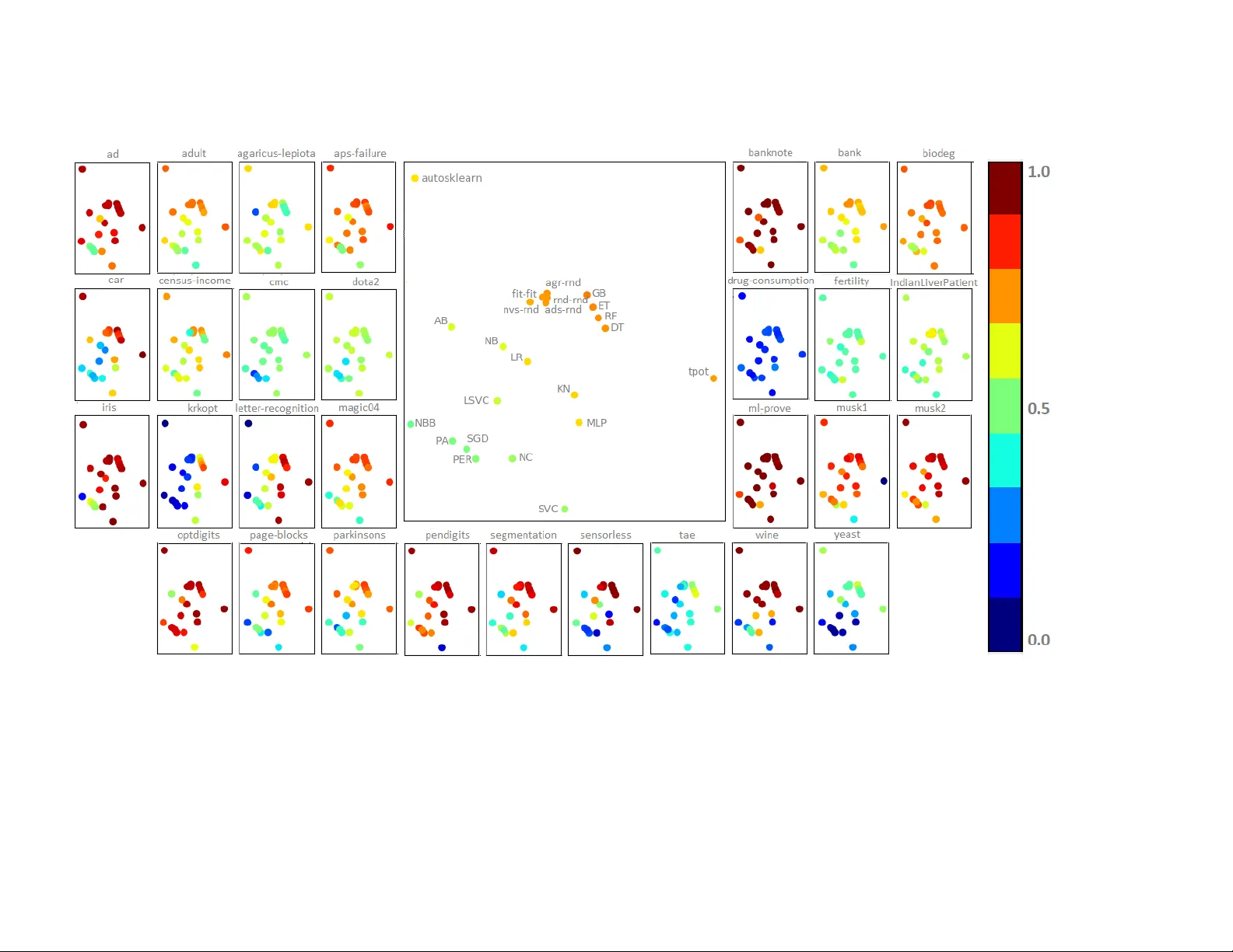
Selection Heuristics on Seman tic Genetic Programming for Classiﬁcation Problems Claudia N. S´ anc hez 1 , 2 Mario Graﬀ 1 , 3 1 INF OTEC Cen tro de Inv estigaci´ on e Inno v aci´ on en T ecnolog ´ ıas de la Informaci´ on y Com unicaci´ on, Circuito T ecnopolo Sur No 112, F racc. T ecnop olo P o citos I I, Aguascalien tes 20313, M´ exico 2 F acultad de Ingenier ´ ıa. Universidad P anamericana, Aguascalientes, M ´ exico 3 CONA CyT Consejo Nacional de Ciencia y T ecnolog ´ ıa, Direcci´ on de C´ atedras, Insurgen tes Sur 1582, Cr´ edito Constructor, Ciudad de M´ exico 03940 M´ exico This w ork has b een submitted to the Ev olutionary Computation journal for p ossible publication. Abstract Individual’s semantics ha ve b een used for guiding the learning pro cess of Genetic Pro- gramming solving sup ervised learning problems. The semantics has been used to prop osed no vel genetic operators as well as diﬀeren t wa ys of p erforming parent selection. The lat- ter is the fo cus of this con tribution by prop osing three heuristics for paren t selection that replace the ﬁtness function on the selection mechanism en tirely . These heuristics comple- men t previous work by b eing inspired in the c haracteristics of the addition, Naiv e Bay es, and Nearest Centroid functions and applying them only when the function is used to cre- ate an oﬀspring. These heuristics use diﬀerent similarit y measures among the parents to decide which of them is more appropriate given a function. The similarity functions con- sidered are the cosine similarity , P earson’s correlation, and agreement. W e analyze these heuristics’ p erformance against random selection, state-of-the-art selection sc hemes, and 18 classiﬁers, including auto-machine-learning tec hniques, on 30 classiﬁcation problems with a v ariable n umber of samples, v ariables, and classes. The result indicated that the combination of paren t selection based on agreemen t and random selection to replace an individual in the p opulation pro duces statistically better results than the classical selection and state-of-the-art sc hemes, and it is competitive with state-of-the-art classiﬁers. Finally , the co de is released as op en-source soft ware. 1 In tro duction Classiﬁcation is a sup ervised learning problem that consists of ﬁnding a function that learns the relation b etw een inputs and outputs, where the outputs are a set of lab els. It could b e applied for solving problems like ob ject recognition, medical diagnosis, identiﬁcation of symbols, among others. The starting p oin t would b e the training set comp osed of input-output pairs, i.e., X = { ( ~ x 1 , y 1 ) , . . . , ( ~ x n , y n ) } , where ∀ ~ x ∈X ~ x ∈ R m , and ∀ y ∈X y ∈ R . The training set X is used to ﬁnd a function, f , that minimize a loss function, L , that is, f is the function that minimize P ( ~ x,y ) ∈X L ( f ( ~ x ) , y ), where the ideal scenario would b e ∀ ( ~ x,y ) ∈X f ( ~ x ) = y , and, also to accurately predict the lab els of unseen inputs. Genetic programming (GP) is a ﬂexible and p o w erful ev olutionary tec hnique with some features that can b e very v aluable and suitable for the ev olution of classiﬁers (Esp ejo et al., 2010). The ﬁrst do cumen t related to GP w as presented b y F riedb erg (1958), but the term was coined b y Koza (1992). The classiﬁers constructed with 1 GP started app earing around the 2000s (Lov eard and Ciesielski, 2001; Brameier and Banzhaf, 2001), and now adays, they can be comparable with state-of-the-art machine learning techniques for solving hard classiﬁcation problems. F or example, GP has b een used for medical prop oses (Brameier and Banzhaf, 2001; Olson et al., 2016), image classiﬁcation (Iqbal et al., 2017), fault classiﬁcation (Guo et al., 2005), only to men tion some of them. Also, the GP p erformance has b een successfully compared with others machine learning techniques as Neural Net works (Brameier and Banzhaf, 2001), Support V ector Mac hines (Lic ho dzijewski and Heyw o od, 2008; McIn tyre and Heyw o o d, 2011). Sp eciﬁcaly , GP can be applied in the prepro cessing task (Guo et al., 2005; Badran and Rock ett, 2012; Ingalalli et al., 2014; La Ca v a et al., 2019), in mo del extraction (Lov eard and Ciesielski, 2001; Brameier and Banzhaf, 2001; Muni et al., 2004; Zhang and Smart, 2006; F olino et al., 2008; McInt yre and Heywoo d, 2011; Graﬀ et al., 2016; Iqbal et al., 2017), or for building mac hine learning pip elines (Olson et al., 2016). T raditionally , GP uses individuals’ ﬁtness to select the parents that build the next generation of individuals (Poli et al., 2008). Recently , new approaches for paren t selection that use angles among individuals’ semantics ha ve been developed. F or example, Angle-Driven Selection (ADS), prop osed by Chen et al. (2019), chooses paren ts maximizing the angle betw een their relative seman tics aiming to hav e paren ts with diﬀeren t b eha viors. V annesc hi et al. (2019) in tro duced a selection scheme based on the angle betw een the error v ectors. Besides, there ha ve b een approaches that analyze evolutiv e algorithms’ b ehavior where the ﬁtness function is replaced with a heuristic. Nguy en et al. (2012) prop osed Fitness Sharing, a technique that promotes dispersion and diversit y of individuals. Lehman and Stanley (2011) proposed Nov elty Search, where the individual’s ﬁtness is related totally to its no velt y without care ab out its target b ehavior. The individual’s no velt y is computed as the a verage distance b et ween its b eha vior and its k -nearest neigh b ors’ b ehavior. Naredo et al. (2016) used No velt y Searc h in GP for solving classiﬁcation problems. How ever, one of the main c haracteristics of GP is that the function set deﬁnes its search space, and to the b est of our knowledge, there are not do cuments that prop ose the use of functions’ prop erties for parent selection. The in tersection b et w een our prop osal and the previous research w orks is on the selection stage of the evolutionary pro cess. Most of the proposed metho ds pro duce a selection mec hanism that considers the semantics of individuals as w ell as the individual’s ﬁtness to choose the parents. The exception is the prop osals using No velt y Searc h, where the selection pro cess is en tirely performed using the semantics. It enhances p opulation div ersit y . Our approac h follo ws this path by aban- doning the ﬁtness function in the selection pro cess. The diﬀerence with Nov elt y Search is that our prop osal searc hes for individuals whose semantics migh t help the function used to create the oﬀ- spring. Besides, once the individual w as created, lo cal optimization is p erformed using the training outputs, or, traditionally named, the target seman tics. F unctions’ prop erties inspire our s election heuristics; in particular, these were inspired b y the addition and the classiﬁers Naive Bay es and Nearest Centroid. The prop osed heuristics measure the similarity among parents. They are based on cosine similarity , Pearson’s correlation co eﬃcien t, and agreemen t 1 . Sp eciﬁcally , our heuristic based on P earson’s correlation co eﬃcien t is quite similar to ADS, but the diﬀerence is that our prop osal is applied only to sp eciﬁc functions. In this do cumen t, w e presen t the comparison of the use of ADS and our prop osal. The selection heuristics are tested on a steady-state GP called EvoD AG. It w as inspired by the Geometric Seman tic genetic operators proposed by Moraglio et al. (2012) with the implemen tation of V annesc hi et al. (V annesc hi et al., 2013; Castelli et al., 2015a). It has b een successfully applied to a v ariet y of text classiﬁcation problems (Graﬀ et al., 2020). In steady-state evolution, the selection mechanism is used twice to p erform parent selection and decide the individual b eing replaced by an oﬀspring; w e refer to the later negativ e selection. The proposed selection is used to select the paren t; ho w ever, on the negativ e selection, w e also tested the system’s p erformance using random selection or the traditional selection guided by ﬁtness. W e analyze the performance of diﬀeren t GP systems obtained by combining the schemes for paren t selection (our heuristics, random selection, and traditional selection) and negative selec- 1 W e thank the anon ymous reviewer for suggesting this name whic h considerably impro ves the description clarit y . 2 tion (random and traditional selection). Besides, w e compare our selection heuristics against t wo state-of-the-art tec hniques, Angle-Driv en-Selection (Chen et al., 2019), and Nov elty Search (Naredo et al., 2016). T o pro vide a complete picture of the performance of our selection heuris- tics, w e decided to compare them against state-of-the-art classiﬁers and t wo auto-machine learning algorithms. The results show that our selection heuristic guided by agreement and random neg- ativ e selection outp erforms traditional selection, presenting a statistically signiﬁcan t diﬀerence. On the other hand, our selection heuristics outp erforms the state-of-the-art tec hniques Angle- Driv en-Selection and Nov elty Search. F urthermore, compared with state-of-the-art classiﬁers, our GP system obtained the second-lo w est rank b eing the ﬁrst one TPOT, an auto-machine learning tec hnique, although the diﬀerence in performance betw een these systems, in terms of macro-F1, is not statistically signiﬁcant. The rest of the manuscript is organized as follo ws. Section 2 presen ts the related w ork. The GP system used to test the prop osed heuristics is described in Section 3. The prop osed selection heuristics are presented in Section 4. Section 5 presents the exp erimen ts and results. The discus- sion and limitations of the approach are treated in Section 6. Finally , Section 7 concludes this researc h. 2 Related w ork W e can deﬁne sup ervised learning as follo ws V annesc hi (2017): given the training set composed of input-output pairs, X = { ( ~ x 1 , y 1 ) , . . . , ( ~ x n , y n ) } , where ∀ ~ x ∈X ~ x ∈ R m , and ∀ y ∈X y ∈ R ; the learning pro cess can b e deﬁned as the problem of ﬁnding a function f that minimizes a loss function, L , that is, f is the function that minimize P ( ~ x,y ) ∈X L ( f ( ~ x ) , y ), where the ideal scenario w ould b e ∀ ( ~ x,y ) ∈X f ( ~ x ) = y . T raditionally , the vector composed by all the outputs, ~ t = { y 1 , . . . , y n } , is called target vector. In this wa y , a GP individual P can be seen as a function h that, for eac h input v ector ~ x i returns the scalar v alue h ( ~ x i ), and the ob jective is to ﬁnd the GP individual that minimizes P ( ~ x,y ) ∈X L ( h ( ~ x ) , y ). On Seman tic Genetic Programming (SGP), for example in (V annesc hi, 2017), eac h individual P can b e represen ted by its seman tics vector ~ S p that corresp onds to all the inputs’ ev aluations in the function h , this is, ~ S p = { h ( ~ x 1 ) , . . . , h ( ~ x n ) } . W e can imagine the existence of t wo spaces: the genotype space, where individuals are represen ted b y their structures, and the phenotype or seman tic space, where individuals are represen ted b y p oin ts, whic h are their semantics. Remark that the target vector ~ t is a p oint in the semantic space. The dimensionality of the semantic space is the n umber of input v ectors. Using this notation, the ob jectiv e of SGP is to ﬁnd the individual P whose semantics S p is as close as p ossible to the target v ector ~ t in the semantic space. The distance betw een the individual’s semantics ~ S p and the target v ector ~ t is used as the individual’s ﬁtness. In order to provide a complete picture of the research documents related to this con tribution, the section starts by describing seman tic genetic operators; this is follo w ed b y presenting research prop osals proposing selection mec hanisms; and, lastly , some prop osals where GP has been used to dev elop classiﬁers. 2.1 Seman tic Genetic Op erators Seman tic Genetic Programming uses the target b eha vior, ~ t , to guide the search. Kra wiec (2016) aﬃrmed that seman tically aw are methods make search algorithms b etter informed. Sp eciﬁcally , sev eral crossov er and mutation op erators ha ve been developed with the use of seman tics. Beadle and Johnson (2008) prop osed a crosso v er operator that measures the semantic equiv alence betw een paren ts and oﬀsprings and rejects the oﬀspring that is semantically equiv alent to its paren ts. Uy et al. (2011) developed a semantic crosso ver and a m utation op erator. The crossov er op erator searc hes for a crossov er p oin t in each parent so that subtrees are semantically similar, and the m utation op erator allows the replacement of an individual’s subtree only if the new subtree is 3 seman tically similar. Hara et al. (2012) prop osed the Semantic Con trol Crossov er that uses se- man tics to com bine individuals. A global searc h is p erformed in the ﬁrst generations and a local searc h in the last ones. Graﬀ et al. used subtrees seman tics and partial deriv atives to prop ose a crosso ver (Graﬀ et al., 2014b; Su´ arez et al., 2015) and a m utation (Graﬀ et al., 2014a) op erator. Moraglio et al. prop osed the Geometric Semantic Genetic Programming (GSGP) (Moraglio and P oli, 2004; Moraglio et al., 2012). Their w ork called the GP scientiﬁc comm unit y’s attention b ecause the crosso ver operator pro duces an oﬀspring that stands in the segmen t joining the par- en ts’ seman tics. Therefore, oﬀspring ﬁtness cannot be worse than the worst ﬁtness of the parents. Giv en t wo parents’ semantics ~ p 1 and ~ p 2 , the crossov er operator generates an oﬀspring whose se- man tics is r · ~ p 1 + (1 − r ) · ~ p 2 , where r is a real v alue b et ween 0 and 1. This prop ert y transforms the ﬁtness landscape into a cone. Unfortunately , the oﬀspring is alwa ys bigger than the sum of its paren ts’ size; this mak es the op erator unusable in practice. Later, some op erators were developed to impro ve Moraglio’s GSGP . F or example, Approximately Geometric Seman tic Crossov er (SX) (Kra wiec and Lichocki, 2009), Deterministic Geometric Seman tic Crosso ver (Hara et al., 2012), Lo cally Geometric Crosso ver (LGX) (Kra wiec and P awlak, 2012, 2013), Appro ximated Geomet- ric Crosso ver (A GX) (P awlak et al., 2015), and Subtree Seman tic Geometric Crossov er (SSGX) (Nguy en et al., 2016). Graﬀ et al. (2015b) prop osed a new crosso ver op erator based on pro jections in the phenot yp e space. It creates a plane in the semantic space using the parents’ semantics. The oﬀspring is calculated as the pro jection of the target in that plane. Given the parents’ semantics ~ p 1 and ~ p 2 , and the target seman tics ~ t , the oﬀspring is calculated as α ~ p 1 + β ~ p 2 , where α and β are real v alues that are calculated solving the equation A [ α, β ] 0 = ~ t , where A = ( ~ p 1 , ~ p 1 ). It implies the oﬀspring will b e at least as goo d as the b est parent. Memetic Genetic Programming based on Orthogonal Pro jections in the Phenotype Space was also prop osed by Graﬀ et al. (2015a). In that w ork, they used a linear com bination of k paren ts as P k α k ~ p k , where ~ p k represen ts the semantics of the k parent. The main idea is optimizing the co eﬃcien ts { α i } with ordinary least squares (OLS) to guarantee that the oﬀspring is the b est of its family . As a result, the generated tree’s ﬁtness is alwa ys b etter or equal to any in ternal tree. It was not the ﬁrst time that parameters w ere added to GP no des; Smart and Zhang (2004) deﬁned the Inclusion F actors as numeric v alues b et w een 0 and 1 assigned to eac h no de in the tree structure, except the ro ot no de. This v alue represen ts the inclusion prop ortion of the no de in the tree. Castelli et al. (2015b) presen ted a m utation op erator, in their w ork called Geometric Seman tic Genetic Programming with Lo cal Searc h, based on Moraglio’s m utation op erator, that also uses parameters. In this operator, an individual’s seman tics ~ p is mo diﬁed with the follo wing equation, α 0 + α 1 ~ p + α 2 ( ~ r 1 − ~ r 2 ), where ~ r 1 and ~ r 2 are the semantics of random trees, and, α i  R . { α i } are calculated using the target seman tics and OLS for getting the b etter linear combination of the individual’s semantics and the random trees. They extended their work in (Castelli et al., 2019) applying Lo cal Search to all the individuals during a separate step after m utation and crosso v er. F or each individual, p , they calculated another one as p 0 = αp + β , where α and β are optimized with OLS minimizing the error b et ween the individual’s semantics and target semantics. Moreo ver, they generalized the idea and transformed it into a regression problem p 0 = P j α j f j ( p ), where f j : R → R . All those op erators use semantics to guide the learning pro cess; ho wev er, one of the main c haracteristics of GP is that the function set deﬁnes its search space, and to the b est of our kno wledge, there are not do cumen ts that prop ose the use of functions’ prop erties for designing op erators. 2.2 Fitness and Selection in Genetic Programming According to V anneschi et al. (2014), one wa y to promote diversit y in GP is b y using diﬀerent selection schemes. Nguy en et al. (2012) prop osed Fitness Sharing, a technique that promotes disp ersion and div ersity of individuals. Their prop osal consisted of calculating an individual’s shared ﬁtness as f 0 i = f i ( m i + 1), where f i is the individual’s ﬁtness, and m i is approximately equal to the n umber of individuals that b eha ve similarly to individual i . Galv an-Lop ez et al. (2013) applied crossov er only to those individuals whose diﬀerence in b eha vior is greater than a 4 deﬁned threshold for ev ery elemen t on the semantic v ectors. Hara et al. prop osed Deterministic Geometric Seman tic Crossov er (Hara et al., 2012), and later, they prop osed to select the paren ts in such a w ay that the line connecting them is as close as possible to the target in the semantic space (Hara et al., 2016). Rub erto et al. (2014) deﬁned the Error V ector and Error Space. The individual error vector ~ e p is deﬁned as ~ e p = ~ p − ~ t , where ~ p is the individual’s seman tics and ~ t represen ts the target seman tics. The error space contains all the individuals represented b y their error v ectors, where ~ t is the origin. The prop osal is to search, in the error space, for t wo or three individuals aligned, instead of using the ﬁtness function; the rationalit y comes from the fact that given the aligned individuals, then there is a straigh tforward procedure to compute the optimal solution. Ch u et al. (2016, 2018) used the error vectors and the Wilco xon signed-rank test to decide whether to select the ﬁttest or the smaller individual as a parent. Their results show that the prop osed tec hniques aim to enhance seman tic diversit y and reduce the co de bloat in GP . V annesc hi et al. (2019) in tro duced a selection sc heme based on the angle b etw een the error v ectors. Chen et al. (2019) prop osed Angle-Driv en Geometric Seman tic Genetic Programming (ADGSGP). Their work attempts to further explore the geometry of geometric op erators in the search space to impro ve GP for symbolic regression. Their prop osal included Angle-Driv en Selection (ADS) that selects a pair of parents that ha ve go od ﬁtness v alues and are far aw ay from eac h other regarding the angle-distance of their relativ e semantics. The ﬁrst parent is selected using ﬁtness, and the second one is chosen maximizing the relative angle-distance b etw een its semantics and the seman- tics of the ﬁrst parent. The angle-distance is deﬁned as γ r = arccos( ( ~ t − ~ p 1 )( ~ t − ~ p 2 ) || ~ t − ~ p 1 |||| ~ t − ~ p 2 || ), where ~ t , ~ p 1 , and ~ p 2 , represent the target seman tics, and seman tics of the ﬁrst and the second paren t, resp ec- tiv ely . Also, they prop osed Perpendicular Crossov er (PC) and Random Segment Mutation (RSM) that likewise used angles to guide their pro cess. Their experiments show that the angle-driven geometric op erators drive the ev olutionary pro cess to ﬁt the target seman tics more eﬃcien tly and impro ve the generalization p erformance. Our prop osal, as well as these do cumen ts, aims to promote individuals’ div ersity but uses functions’ properties for guiding the paren t selection. 2.3 Genetic Programming for classiﬁcation Genetic programming (GP) is a ﬂexible and p ow erful ev olutionary tec hnique with some features that can b e v ery v aluable and suitable for the evolution of classiﬁers (Esp ejo et al., 2010). F or example, GP has b een used for medical prop oses (Brameier and Banzhaf, 2001; Olson et al., 2016), image classiﬁcation (Iqbal et al., 2017), and fault classiﬁcation (Guo et al., 2005). Also, GP classiﬁers hav e b een successfully compared with state-of-the-art classiﬁers. Brameier and Banzhaf (2001) compared GP against neural netw orks on medical classiﬁcation problems from a benchmark database. Their results sho w that GP performs comparably in classiﬁcation and generalization. McIn tyre and Heywoo d (2011) compared their GP framework against SVM classiﬁers ov er 12 UCI datasets with b et ween 150 and 200,000 training instances. Solutions from the GP framew ork app ear to provide a go o d balance b etw een classiﬁcation p erformance and model complexity , espe- cially as the dataset instance coun t increases. La Cav a et al. (2019) compared their GP framew ork to several state-of-the-art classiﬁcation techniques (Random F orest, Neural Net works, and Sup- p ort V ector Machines) across a broad set of problems, and show ed that their technique achiev es comp etitiv e test accuracies while also pro ducing concise mo dels. Data can b e transformed at the prepro cessing stage to increase the quality of the kno wledge obtained, and GP can b e used to p erform this transformation (Espejo et al., 2010). Badran and Ro c k ett (2012) prop osed multi-ob jectiv e GP to evolv e a feature extraction stage for multiple-class classiﬁers. They found mappings that transform the input space in to a new multi-dimensional decision space to increase the discrimination betw een all classes; the num b er of dimensions of this decision space is optimized as part of the ev olutionary pro cess. Ingalalli et al. (2014) introduced a GP framew ork called Multi-dimensional Multi-class Genetic Programming (M2GP). The main idea is to transform the original space into another one using functions ev olved with GP , then, a 5 cen troid is calculated for each class, and the v ectors are assigned to the class that corresp onds to the nearest centroid using the Mahalanobis distance. M2GP tak es as an argument the dimension of the transformed space. This parameter is evolv ed in M3GP (Munoz et al., 2015) by including sp ecialized searc h operators that can increase or decrease the n umber of feature dimensions pro- duced b y each tree. They extended M3GP and prop osed M4GP (La Cav a et al., 2019) that uses a stack-based represen tation in addition to new selection methods, namely lexicase selection and age-ﬁtness P areto surviv al. Naredo et al. (2016) used Nov elty Search (NS) for evolving GP classiﬁers based on M3GP , where the diﬀerence is the procedure to compute the ﬁtness. Each GP individual is represen ted as a binary v ector whose length is the training set size, and each v ector element is set to 1 if the classiﬁer assigns the class lab el correctly and 0 otherwise. Then, those binary vectors are used to measure the sparseness among individuals, and the more the sparseness, the higher the ﬁtness v alue. Their results show that all their NS v ariants ac hieve comp etitive results relative to the traditional ob jectiv e-based. Auto machine learning consists of obtaining a classiﬁer (or a regressor) automatically . It includes the steps of prepro cessing, feature s election, classiﬁer selection, and hyperparameters tuning. F eurer et al. (2015) dev elop ed a robust automated mac hine learning (AutoML) technique using Bay esian optimization metho ds. It is based on scikit-learn (Pedregosa et al., 2011), using 15 classiﬁers, 14 feature preprocessing methods, and 4 data prepro cessing metho ds; giving rise to a structured h yp othesis space with 110 hyperparameters. Olson et al. (2016) prop osed the use of GP to dev elop an algorithm that automatically constructs and optimizes machine learning pip elines through a T ree-based Pipeline Optimization T o ol (TPOT). On classiﬁcation, the ob jective consists of maximizing the accuracy score p erforming a searc hing of the combinations of 14 prepro cessors, ﬁv e feature selectors, and 11 classiﬁers; all these tec hniques are implemented on scikit-learn. It is in teresting to note that TPOT uses a tree-based GP programming approach where the diﬀerent learning pro cess comp onents are no des in a tree, and traditional subtree crossov er is used as a genetic operator. The use of the prop osed selection heuristics improv es EvoD AG, a GP system describ ed in Section 3, making it competitive with the auto-machine learning tec hniques explained abov e and other state-of-the-art classiﬁers. 3 Genetic Programming System W e decided to implement the prop osed selection heuristics and the selection heuristics of the state-of-the-art in our previously developed GP system called EvoD AG 2 (Graﬀ et al., 2016, 2017). Ev oDA G is inspired b y the implementation of GSGP performed by Castelli et al. (2015a), where the main idea is to keep trac k of all the individuals and their b ehavior, leading to an eﬃcient ev aluation of the oﬀspring whose complexity depends only on the n umber of ﬁtness cases. Let us recall that the oﬀspring, in the geometric seman tic crossov er, is ~ o = r ~ p 1 + (1 − r ) ~ p 2 , where r is a random function or a constan t, and, ~ p 1 and ~ p 2 are the parents’ seman tics. As it w as explained in the previous section, in (Graﬀ et al., 2015b), w e decided to extend this operation b y allowing the oﬀspring to b e a linear combination of the paren ts, that is, ~ o = θ 1 ~ p 1 + θ 2 ~ p 2 , where θ 1 and θ 2 are obtained using ordinary least squares (OLS) minimizing the diﬀerence betw een the oﬀspring and the target semantics. Contin uing with this line of researc h, in (Graﬀ et al., 2016), w e in vestigated the case when the oﬀspring is a linear combination of more than tw o parents, and, also, to include the possibility that the parents could be combined using a function randomly selected from the function set. Ev oDA G, as customary , uses a function set F = { P 60 , Q 20 , max 5 , min 5 , √ · , | · | , sin, tan, atan, tanh, h yp ot 2 , NB 5 , MN 5 , NC 2 } , and a terminal set T = { x 1 , . . . , x m } , to create the indi- viduals. It is also included in F classiﬁers suc h as Naiv e Ba yes with Gaussian distribution (NB 5 ), with Multinomial distribution (MN 5 ), and Nearest Centroid (NC 2 ). The function-set elements are traditional op erations where the subscript indicates the n umber of arguments. EvoD A G’s 2 https://gith ub.com/mgraﬀg/EvoD AG 6 default parameters, including the num b er of arguments, were deﬁned p erforming a random search (Bergstra and Bengio, 2012), on the parameter space, using as a b enc hmark of classiﬁcation prob- lems that included diﬀerent sen timent analysis problems as well as problems taken from UCI rep ository (not included in the problems used to measure the p erformance of the selection heuris- tics). The ﬁnal v alues were the consensus of the parameters obtaining the b est p erformance in the problems tested. The initial p opulation starts with P = { θ 1 x 1 , . . . , θ m x m , NB( x 1 , . . . , x m ), MN( x 1 , . . . , x m ), NC( x 1 , . . . , x m ) } , where x i is the i -th input, and θ i is obtained using OLS. In the case that the num- b er of individuals is low er than the p opulation size, the pro cess starts including an individual cre- ated by randomly selecting a function from F and the arguments are drawn from the current p op- ulation P . F or example, let hypot b e the selected function, and the ﬁrst and second argumen ts are θ 2 x 2 , and NB( x 1 , . . . , x m ). Then, the individual inserted to P is θ h yp ot( θ 2 x 2 , NB( x 1 , . . . , x m )), where θ is obtained using OLS. This pro cess contin ues until the population size is reached; Ev oDA G sets population size of 4000. Ev oDA G uses a steady-state evolution; consequently , P is up dated by replacing a current individual, selected using a negativ e selection, with an oﬀspring that can b e selected as a paren t just after b eing inserted in P . The evolution pro cess is similar to the one used to create the initial p opulation, and the diﬀerence is in the pro cedure used to select the ar guments. That is, a function f is selected from F , its arguments are selected from P using tournament selection or any of the prop osed selection heuristics, and ﬁnally , the parameters θ asso ciated to f are optimized using OLS. The addition is deﬁned as P i θ i x i , where x i is an individual in P . The rest of the arithmetic functions, trigonometric functions, min, and max are deﬁned as θ f ( . . . , x i , . . . ), where f is the function at hand, and x i is an individual in P . F or preven ting ov erﬁtting, EvoD AG stops the ev olutionary process using early stopping; that is, the training set is split into a smaller training set (50% reduction) and a v alidation set con taining the remaining elements. The training set is used to calculate the ﬁtness and the parameters θ . The evolution stops when the best individual on the v alidation set has not b een updated in a deﬁned num b er of ev aluations; Ev oDA G sets this as 4000. The ﬁnal mo del corresp onds to the b est individual in the v alidation set found during the whole ev olutionary pro cess. A t this point, it is worth mentioning that EvoD AG uses a one-vs-rest scheme on classiﬁcation problems. That is, a problem with k diﬀerent classes is conv erted into k problems; each one assigns 1 to the current class and − 1 to the other labels. Instead of ev olving one tree p er class, as done, for example, in Muni et al. (2004), w e decided to use only one tree and optimize k diﬀeren t θ parameters, one for each lab el. The result is that each no de outputs k v alues, and the class is the one with the highest v alue. In the no des represen ting classiﬁers, like Naiv e Ba yes or Nearest Centroid, the output is the log-likelihoo d. In order to provide an idea of the type of mo dels pro duced by Ev oDA G, Figure 1 presents a mo del of the Iris dataset. The inputs ( x 0 , . . . , x 3 , NB , MN , NC) are at the bottom of the ﬁgure. The computation ﬂow goes from b ottom to top; the output node is at the top of the ﬁgure, i.e., Naive Ba yes using Gaussian distribution. The ﬁgure helps to understand the role of optimizing the k set of parameters, one for each class, where eac h node outputs k v alues; consequently , each no de is a classiﬁer. Ev oDA G uses macro- F1 score to calculate the individuals’ ﬁtness. The macro-F1 score w as chosen because it helps to handle im balanced datasets. The class imbalance problem t ypically o ccurs when, in a classiﬁcation problem, there are many more instances of some classes than others. In such cases, standard classiﬁers tend to b e ov erwhelmed by the class with more examples ignoring the less represen ted classes (Cha wla et al., 2004). It is well kno wn that in evolutionary algorithms, there are runs that do not pro duce an ac- ceptable result, to improv e stabilit y , w e decided to use Bagging (Breiman, 1996) in our approac h. W e create 30 diﬀeren t mo dels b y randomly selecting 50% samples for training and the remain- ing for v alidation. A bagging estimator can be exp ected to p erform similarly b y either dra wing n elements from the training set with-replacement or selecting n 2 elemen ts without-replacemen t (F riedman and Hall, 2007). In addition, we reduce the learning complexit y that, in Ev oDA G’s case, is measured in terms of training samples. Ev oDA G’s ﬁnal prediction is the av erage of the mo dels’ predictions. 7 Figure 1: A mo del evolv ed b y Ev oD AG on the Iris dataset. The inputs are in the b ottom of the ﬁgure and the output is on the top. 4 Selection Heuristics This do cumen t prop oses selection heuristics for GP tailored to classiﬁcation problems based on the idea that functions’ prop erties and individuals’ seman tics can guide parent selection. The heuristics replace the ﬁtness function used in the selection pro cedure - tested in particular in tournamen t selection - to select the paren t. Let us recall that in a steady-state evolution, there are tw o stages where selection takes place. On the one hand, the selection is used to choose the paren ts, and on the other hand, the selection is applied to decide which individual, in the curren t p opulation, is replaced by the oﬀspring. This last one is called negative selection. The most p opular selection method in GP is tournamen t selection (F ang and Li, 2010), and also, negative selection is commonly p erformed using the same selection scheme; nonetheless, in the latter case, the winner of the tournament is the one with the worst ﬁtness. In the rest of the section, w e describ e the pro cess of creating an oﬀspring in EvoD A G, and the traditional tournament selection (based on ﬁtness), random selection, and our three prop osed selection heuristics. In Ev oDA G, the pro cess of creating an oﬀspring starts b y selecting a function from the function set F , and then parent selection needs to be p erformed to c ho ose each one of the k argumen ts (or paren ts). Figure 2 sho ws an example of the traditional tournamen t selection (with tournament size t wo) where the function P w as selected, and 3 individuals need to be selected as argumen ts from the population P for creating the new oﬀspring. It can b e seen that for selecting each argumen t, a binary tournament needs to be performed. F or selecting an argument, tw o individuals from the p opulation are randomly chosen, and the one with the highest ﬁtness is selected as the argumen t; eac h tournament is depicted using a diﬀerent color. The pro cedure represen ted in Figure 2 also helps to describ e random selection where eac h argument of the function P is selected randomly from the p opulation, and a tournamen t is not needed. As can be seen, random selection is the most straigh tforward and less expensive strategy giv en that there is no need to perform the tournamen t. Let us start b y describing the selection heuristics that w ere inspired by functions’ prop erties. The functions are the addition and the classiﬁers Naiv e Ba yes and Nearest Cen troid. The addition 8 Figure 2: Diagram of tournament selection using the ﬁtness function to decide the winner of the tournamen t. is deﬁned in our GP system as P k θ k p k , where OLS and target seman tics are used to estimate θ k . As can b e seen, to accurately iden tify the k co eﬃcien ts, the exogenous v ariables p k m ust b e linearly indep enden t. In general, kno wing whether a set of vectors is linearly indep enden t requires a non-zero determinan t; how ev er, the trivial case is when these v ectors are orthogonal. Based on Brereton (2016), uncorrelated vectors are also linearly indep enden t. In Naiv e Bay es’s case, its model assumes that given a class, the features are independent. As exp ected, the process to calculate indep endence is exp ensiv e, so instead, w e use the correlation among features in our heuristic. The correlation of t wo statistically independent v ariables is zero, although the inv erse is not necessarily true. Finally , Nearest Centroid (NC) is a classiﬁer representing each class with its centroid calculated with the elements asso ciated with that class. The lab el of a given instance corresp onds to the class of the closest centroid. Therefore, we think it might improv e the p erformance of NC if the div ersity of the inputs is increased. T o sum up, the three functions (addition, Naiv e Bay es, and Nearest Centroid) p erform better when their input vectors are orthogonal, uncorrelated, or indep enden t. The main idea is quite similar to the proposal in No velt y Searc h (Lehman and Stanley, 2011), where instead of promoting ﬁtness, they promote diversit y . In our case, w e wan t ﬁt individuals for the ﬁnal solution, but w e select parents promoting diversit y among them. The prop osed selection heuristics use the individuals’ seman tics for c ho osing div erse paren ts. The ﬁrst selection heuristic ideally would select orthogonal v ectors; eviden tly , this ev ent is unlik ely , so a function that measures the closeness to orthogonalit y is needed. The cosine similarit y is suc h a measure, it is deﬁned in Equation 1, where ~ v 1 and ~ v 2 are v ectors, · represen ts the dot pro duct, and k ~ v k the norm of ~ v . Its range is b etw een − 1 and 1, where 1 indicates that the v ectors are in the same direction, − 1 exactly the opposite direction, and 0 indicates that v ectors 9 Figure 3: Diagram of paren t selection based on heuristics. are orthogonal. It is worth mentioning that the absolute of the cosine similarit y is used instead b ecause a cosine-similarity v alue of 1 or − 1 is similar regarding the linear indep endence. C S ( ~ v 1 , ~ v 2 ) = cos ( θ ) = ~ v 1 · ~ v 2 k ~ v 1 k k ~ v 2 k (1) The process of selecting a paren t using the absolute cosine similarity is depicted in Figure 3. Let us recall that tournament selection (with a tournamen t size of t wo) is b eing used, and the selection heuristic replaces the ﬁtness function used traditionally in the tournamen t to select the paren ts. Under th is conﬁguration, the ﬁgure depicts the selection of three arguments for b eing used with the addition function. The ﬁrst of the argumen ts is selected randomly from the population; this is depicted on the red box. Selecting the second argumen t (box in green) requires c ho osing t wo individuals from the p opulation randomly and then comparing them using the absolute cosine similarit y b etw een eac h of the selected individuals and the ﬁrst argumen t. The second argument is the one with the low est v alue: the closest to a 90-degree angle. The absolute cosine similarity is obtained using the individuals’ semantics, and these are v ectors or a list of v ectors (in case of m ulti-class problems); in the latter case, the av erage of the absolute cosine similarity is used instead. Finally , selecting the last argumen t (blue box) is equiv alen t to the previous one. That is, the individuals selected from the p opulation are compared using the absolute cosine similarit y with resp ect to the ﬁrst argumen t selected. Although this pro cess do es not guaran tee that all the arguments are unique, the implemen tation ensures that all individuals are diﬀerent; this is depicted in the ﬁgure by representing eac h possible argument with a diﬀerent tree. The second heuristic uses the P erson’s Correlation Co eﬃcien t to select uncorrelated in- puts. The correlation co eﬃcien t is deﬁned in Equation 2, where ~ v 1 and ~ v 2 are v ectors with the v alues of the v ariables, · represen ts the dot pro duct, ¯ ~ v is the a verage v alue of v ector ~ v , and k ~ v k the norm of ~ v . Pearson’s range is b et ween − 1 and 1, where 1 indicates p ositively correlated, 0 represents no linear correlation, and − 1 represents a total negative linear correlation. It can 10 b e observed that Equations 1 and 2 are similar. The diﬀerence is that correlation (Equation 2) subtracts the a verage v alue to the v ectors. It means that the heuristics based on cosine similarity and correlation will b e the same when the data is zero-cen tering. ρ ~ v 1 , ~ v 2 = ( ~ v 1 − ¯ ~ v 1 ) · ( ~ v 2 − ¯ ~ v 2 )   ~ v 1 − ¯ ~ v 1     ~ v 2 − ¯ ~ v 2   (2) Figure 3 depicts the process of selecting three argumen ts for the addition function. The process is similar to the one used for the co sine similarity , being the only diﬀerence b etw een them the use of the absolute v alue of the Pearson’s co eﬃcien t instead of the cosine similarity . That is, the ﬁrst argumen t is selected randomly from the p opulation, whereas the second and third argumen ts are the individuals whose seman tics obtained the lo west absolute P earson’s correlation co eﬃcien t for eac h tournament. The previous selection heuristics increase the v ariety of the inputs using cosine similarit y and P earson’s Correlation coeﬃcient. Ho wev er, these similarities do not consider the prediction lab els. In classiﬁcation problems, the individual’s outputs are transformed to obtain the lab els taking, for example, the maxim um v alue index in a multiple output represen tation. The idea of the last heuristic is to complemen t the previous selection heuristics b y measuring div ersity using the predicted labels; the measure used with this purp ose is named agreement – deﬁned in the Equation 3 3 , where ~ p 1 and ~ p 2 represen t the lab els v ectors of t wo individuals, n is the num b er of samples, and δ ( . ) returns 1 if its input is true and 0 otherwise. ag r ( ~ p 1 , ~ p 2 ) = 1 n X i δ ( p 1 i == p 2 i ) (3) Figure 3 depicts the pro cedure to select three arguments for the addition function using the agreemen t as the selection heuristic. The pro cess is similar to the ones used for the previous selection heuristics. That is, the ﬁrst argumen t is an individual randomly selected from the p opulation. The second and third argument is selected p erforming a tournament where the ﬁtness function is replaced by agreement. F or example, the second argument (green b o x) is selected b y ﬁrst transforming the ﬁrst argument’s outputs into lab els and transforming the outputs of the tw o individuals selected in the tournament. The lab els obtained are used to compute tw o agreemen t v alues, one for eac h individual in the tournamen t using in common the lab els of the ﬁrst argumen t, i.e., the individual selected randomly . The second argumen t selected is the individual with the lo w est agreement, i.e., the one that optimizes the v ariety . The third argumen t is selected p erforming another tournament following an equiv alent metho d used on the second argument. T o sum up, three selection heuristics are prop osed, in this contribution, corresponding to the use of the absolute cosine similarity , P earsons’ Correlation co eﬃcient, and agreement. These heuristics replace the ﬁtness function in the tournament selection pro cedure, and, consequently , the selected individuals are the ones with the low est v alues on the particular heuristic used. 5 Exp erimen ts and results The selection heuristics p erformance is analyzed in this section and compared against our GP system with the default parameters, with state-of-the-art selection heuristics, and with traditional classiﬁers and classiﬁers using full-mo del selection. 5.1 Datasets The classiﬁcation problems used as b enc hmarks are 30 datasets taken from the UCI rep ository (Dua and Graﬀ, 2017). T able 1 shows the dataset information. It can be seen that the datasets are heterogeneous in terms of the num b er of samples, v ariables, and classes. Additionally , some of the classiﬁcation problems are balanced, and others are imbalanced. W e use Shannon’s entrop y to 3 Note that in the case ~ p 2 is the target b eha vior, then the agreement is computing the accuracy of ~ p 1 . 11 indicate the degree of the class-imbalance in the problem. It is deﬁned as H ( X ) = − P i p i log( p i ), where p i represen ts the probability of the category i . W e calculate those probabilities by counting the frequencies of each category . Besides, for normalizing, we use the logarithm base on the n umber of categories. F or example, if the classiﬁcation problem has four categories, w e calculate the Shannon’s entrop y as H ( X ) = − P i p i log 4 ( p i ). In this sense, if the v alue is equal to 1 . 0, it indicates a p erfect balance problem. In opp osite, the smaller the v alue, the bigger the im balance. T able 1: Datasets used to compare the performance of the algorithms. These problems are tak en from the UCI rep ository . The table includes Shannon’s entrop y to indicate the degree of the class- im balance, where the v alue 1 . 0 indicates that the samples are p erfectly balanced. In opp osite, the smaller the v alue, the bigger the imbalance. Dataset T rain T est V ariables Classes Classes samples samples en tropy ad 2295 984 1557 2 0.58 adult 32561 16281 14 2 0.8 agaricus-lepiota 5686 2438 22 7 0.81 aps-failure 60000 16000 170 2 0.12 banknote 960 412 4 2 0.99 bank 31647 13564 16 2 0.52 bio deg 738 317 41 2 0.91 car 1209 519 6 4 0.6 census-income 199523 99762 41 2 0.34 cmc 1031 442 9 3 0.98 dota2 92650 10294 116 2 1.0 drug-consumption 1319 566 30 7 0.44 fertilit y 69 30 9 2 0.43 IndianLiv erPatien t 407 175 10 2 0.85 iris 105 45 4 3 1.0 krk opt 19639 8417 6 18 0.84 letter-recognition 14000 6000 16 26 1.0 magic04 13314 5706 10 2 0.93 ml-pro ve 4588 1530 56 2 0.98 m usk1 333 143 166 2 0.99 m usk2 4618 1980 166 2 0.61 optdigits 3823 1797 64 10 1.0 page-blo c ks 3831 1642 10 5 0.27 parkinsons 135 59 22 2 0.79 p endigits 7494 3498 16 10 1.0 segmen tation 210 2100 19 7 1.0 sensorless 40956 17553 48 11 1.0 tae 105 45 5 3 0.99 wine 123 53 13 3 0.99 y east 1038 446 9 10 0.76 The performance of the classiﬁers is measured in a test set. Some of the problems are already split b et ween a training set and a test set in the rep ository . F or those problems that this partition is not present, w e p erformed cross-v alidation; that is, w e randomly split the dataset using 70% of the samples for the training set and 30% for the test set. 12 5.2 Computer Equipmen t The computer characteristics where the exp eriments were executed are shown in T able 2. F or a fair comparison, the exp erimen ts were executed using only one core. T able 2: Characteristics of the computer where the experiments w ere executed Op erating system Ubun tu 16.04.2 L TS Pro cessor (CPU) In tel (R) Xeon(R) CPU E5-2680 v4 Pro cessor (CPU) sp eed 2.5GHz Computer memory size 256 GB Hard disk size 1 TB Cores n umber 14 5.3 P erformance Metrics The classiﬁers’ p erformance is analyzed in terms of precision and time sp ent on training using tw o metrics: macro-F1 and time (in seconds) p er sample. Accuracy is ma yb e the most used metric for measuring the p erformance of classiﬁers. Its v alue ranges from 0 to 1, being one the b est p erformance and zero the w orst. It can be seen as the p ercen tage of samples that are correctly predicted. How ev er, if the classes are imbalanced, as the problems in this b enc hmark, accuracy is not reliable. On the other hand, the F1 score measures a binary classiﬁer’s performance taking in to account the p ositiv e class. It is robust to im balanced problems. F or a m ulti-class problem, the F1 score can be extended as the macro-F1 score that corresp onds to the av erage of the F1 score per class. Besides, most of the comparisons are performed based on the rank of macro-F1. It means, for eac h dataset, the classiﬁers are rank ed according to their performance. The num b er 1 is assigned to the classiﬁer with the highest v alue in macro-F1, num b er 2 corresp onds to the one with the second-highest v alue in macro-F1, and so on. If several classiﬁers ha ve the same v alue in macro-F1, they got the same rank, and the follo wing rank n umber will b e increased the num b er of repeated v alues. In addition to a classiﬁer’s p erformance for predicting the samples correctly , time is an es- sen tial factor in an algorithm. When the n umber of samples in the training set is small, all the algorithms learn the model quickly . How ever, if the n umber of samples gro ws, some algorithms sp end considerably more and more time, and in some cases, it could b e impossible to wait until the algorithm con verges. As we mention in the previous section, the datasets v ary on the n umber of samples, and, logically , algorithms sp end more time learning big datasets. In that sense, to normalize the time, and with the idea of making comparisons based on this measure, we divided the time (in seconds) that algorithms spend in the training phase by the n umber of samples in the datasets. 5.4 Comparison of the Prop osed Selection Heuristics against Classic T ournamen t Selection W e p erformed a comparison of diﬀerent selection sc hemes for paren t and negative selection. Sp ecif- ically for paren t selection , we compare the use of the following techniques: (1) traditional tourna- men t selection, which uses the individual’s ﬁtness ( ﬁt ), (2) random selection ( rnd ), (3) tournamen t selection with the absolute of cosine similarity ( sim ), (4) tournamen t selection with the absolute of P earson’s correlation co eﬃcien t ( prs ), and, (5) tournamen t selection with the agreemen t ( agr ). The latest three selection metho ds correspond to the proposed selection heuristics; in this case, the selection heuristics are applied only for the functions that inspired them, i.e., addition ( P ), Naive Ba yes (NB and MN), and Nearest Centroid (NC), in the rest of the functions random selection is used instead. In addition, for negative selection , w e analyze the use of the traditional negative 13 selection, which uses the individual’s ﬁtness to select the worst individual in the tournamen t ( ﬁt ), and random selection ( rnd ). The selection schemes were tested on our GP system (Ev oDA G). T o improv e the reading, w e use the following notation. The selection scheme used for paren t selection is follow ed by the sym b ol “-”, and then comes the abbreviation of the negative selection sc heme. F or example, sim-ﬁt means tournamen t selection with the absolute cosine similarit y for paren t selection and traditional negativ e selection are used. In total, w e analyze the performance of eight combinations: ﬁt-ﬁt, rnd- rnd, sim-ﬁt, sim-rnd, prs-ﬁt, prs-rnd, agr-ﬁt, and agr-rnd. F urthermore, to complete the picture of the proposed selection heuristics and the relation with the functions that served as inspiration, w e decided to include in the comparison the p erformance GP systems when the heuristics are used in all the functions with tw o or more argumen ts. These systems are identiﬁed with the symbol *. F or example, agr-rnd indicates that agreemen t is used with the functions P , NB, MN, and NC; whereas, agr-rnd* means that the heuristic is used with the functions: P , Q , max, min, h yp ot, NB, MN, and NC. Figure 4 shows the performance for the diﬀerent techniques used for parent and negative se- lection on classiﬁcation tasks. The detailed results can be observ ed on T able 4. Figure 4a shows the p erformance results based on mac ro-F1 ranks o ver the test sets. It can b e seen that the best p erformance is obtained by selecting the paren ts with the agreemen t heuristic and random nega- tiv e selection (agr-rnd), follow ed by the use of the same scheme for parent selection and negative tournamen t selection (agr-ﬁt). The combinations agr-rnd, agr-ﬁt, sim-ﬁt, prs-ﬁt*, prs-rnd, prs-ﬁt, prs-rnd*, sim-ﬁt*, sim-rnd, and sim-rnd* are b etter than ﬁt-ﬁt (i.e., selection using the ﬁtness function) in terms of macro-F1 a verage rank. It means that our prop osed heuristics impro ve the p erformance of the classical selection sc hemes (ﬁt-ﬁt). Random selection for parent and negativ e selection, rnd-rnd, also improv es the p erformance of Ev oDA G using the classical selection schemes based on ﬁtness (ﬁt-ﬁt). It indicates the imp ortance of p opulation diversit y , as mentioned in Nov- elt y Searc h Lehman and Stanley (2011). Besides, as w e men tion in Section 3, once the individual is created, the function parameters are optimized using OLS and the target semantics. Our heuristic based on agreement works w ell b ecause it is quite similar to the Nov elty Search implemented in (Naredo et al., 2016), but instead of impro ving diversit y among all individuals in the population, it enhances the diversit y among paren ts. F rom the ﬁgure, it can also b e observed that there exists a tendency when the heuristics (iden tiﬁed with the symbol *) are applied to all functions with more than one argument ( P , Q , max, min, hypot, NB, MN, and NC); the results are w orse than those systems that use the prop osed heuristics on the functions that inspired them (i.e., addition, Naive Ba yes and Nearest Cen troid). It aﬃrms the importance of generating heuristics that are speciﬁcally designed based on the functions’ prop erties. Comparing b y the time that the classiﬁers sp end in the training phase (see Figure 4.b), it can b e seen that rnd-rnd is the fastest; this is b ecause it is the most straigh tforward. F or the statistical analysis, w e use the F riedman and Nemenyi tests (Dem ˇ sar, 2006). Macro- F1 ranks v alues were used for the F riedman test where there w as rejected the null hypothesis, with a p-v alue of 4 . 39 e − 22. Based on Nemenyi test, the groups of techniques that are not signiﬁcan tly diﬀerent (at p=0.10) are: Group 1 (agr-rnd, agr-ﬁt, rnd-rnd, sim-ﬁt, prs-ﬁt*, prs-rnd, prs-rnd*, prs-ﬁt, sim-ﬁt*, sim-rnd, and sim-rnd*), Group 2 (agr-ﬁt, rnd-rnd, sim-ﬁt, prs-ﬁt*, prs- rnd, prs-rnd*, prs-ﬁt, sim-ﬁt*, sim-rnd, sim-rnd*, and ﬁt-ﬁt), and Group 3 (agr-rnd*, agr-ﬁt*). It indicates that our prop osed heuristic com bination based on the agreement for paren t selection and random negativ e selection (agr-rnd) performs statistically b etter than the classical tournamen t selection using ﬁtness (ﬁt-ﬁt) b ecause they b elong to diﬀerent groups, i.e., Group 1 and Group 2, resp ectiv ely . The test also indicates that there is not enough evidence to diﬀerentiate the systems of Group 2 (except ﬁt-ﬁt) with system agr-rnd. 14 (a) (b) Figure 4: Selection schemes comparison. a) Macro-F1 ranks that are measured ov er the test datasets. b) Time, in seconds, required b y the diﬀeren t selection tec hnique combinations in the training phase. The time is divided by the num b er of train samples in the datasets. In b oth ﬁgures, green boxplots represent where the selection heuristics (sim, prs, or agr) are applied to all functions. The av erage rank, or time p er sample, sorts the classiﬁers, and it appears on the left. 15 5.5 Comparison of the Proposed Selection Heuristics against State-of- the-Art Selection Sc hemes As we men tion in Section 2, there are selection heuristics related to this research. Consequently , w e decided to compare our selection heuristics with the tw o most similar metho ds; these are Angle-Driv en-Selection (Chen et al., 2019) and Nov elt y Search (Lehman and Stanley, 2011). In Angle-Driv en Selection (ads), the ﬁrst individual is selected using traditional tournamen t selection and then replaces the ﬁtness function, in the tournament selection, with their relative angle in the error space. As can b e seen, in Angle-Driv e-Selection, the ﬁrst individual is chosen using the ﬁtness, whereas, in our prop osal, it is selected randomly . Therefore, we decided to add another parameter to indicate whether the ﬁrst individual is selected using the ﬁtness (ﬁt) or random (rnd). The combinations of selection tec hniques’ notation is as follows. The sym b ol “-” follo ws the parent selection technique, then comes the abbreviation of the negative selection scheme, and, for our heuristics and ads, at the ending, after the sym b ols “–”, comes the abbreviation of the sc heme to select the ﬁrst individual. F or example, agr-rnd–ﬁt means that agreemen t is used for paren t selection, the negativ e selection is p erformed randomly , and the ﬁrst individual is selected using the ﬁtness. Figure 5: Proposed heuristics against state-of-the-art selection schemes based on macro-F1. Bo x- plots present the ranks, and those are measured using macro-F1 o ver the test datasets. Gray b o xplots represent the selection techniques from the state-of-the-art, Nov elty Searc h (n vs) and Angle-Driv en Selection (ads). The av erage rank sorts the classiﬁers, and it appears on the left. Figure 5 presen ts the results of the comparison, based on macro-F1, of our prop osed heuristics, agreemen t, P earson’s Correlation co eﬃcien t, and cosine similarity (agr, prs, and sim) against state- of-the-art selection tec hniques: Angle-Driven Selection (ads) and Nov elty Search (nvs). T ables 5 and 6 show the detailed results. It can b e observ ed that the p erformance of our heuristics is generally b etter than Angle-Driv en Selection (ads) and Nov elty Search (n vs). Using F riedman and 16 Nemen yi tests (Dem ˇ sar, 2006), it was found that agr-rnd–rnd, agr-ﬁt–ﬁt, agr-ﬁt–rnd, rnd-rnd, sim- ﬁt–rnd, agr-rnd–ﬁt, prs-ﬁt–rnd, prs-rnd–rnd, ads-rnd–rnd, and sim-rnd–rnd are not signiﬁcantly diﬀeren t (at p = 0.10), but agr-rnd–rnd is signiﬁcantly b etter than no velt y search (nvs-rnd), angle-driv en with the original prop osal of selecting the ﬁrst individual at random (ads-ﬁt–ﬁt), ﬁt-ﬁt, ads-rnd–rnd*, and ads-ﬁt–ﬁt*. In the original proposal of Angle-Driv en selection (Chen et al., 2019), it is implemen ted in a Geometric Semantic GP system. Ho wev er, in this case, it is applied in EvoD AG. Angle-Driv en selection is quite similar to the prop osed heuristics based on Pearson’s Correlation co eﬃcien t and cosine similarity (alb eit following a diﬀerent path). These tec hniques use the geometry of individuals’ seman tics for parent selection. ADS measures the angle b et ween relativ e seman tics (see Section 2), while our heuristics measure the angle b et w een the semantics and the centered seman tics (see Section 4). On Figure 5, it can be observed that Angle-Driven selection (ads-rnd– rnd) performs similar to P earson’s Correlation coeﬃcient (prs-rnd–rnd) and cosine similarit y (sim- rnd–rnd); in fact, its rank is in the middle of these tw o systems. Besides, Angle-Drive Selection is b etter when it uses the combination of selection sc hemes ads-rnd–rnd than the original proposal ads-ﬁt–ﬁt. As our heuristics behavior, w e can see that Angle-Driv e Selection works b etter when applied only to the functions addition, Naive Ba yes, and Nearest Cen troid than when applied to all functions with more than one argumen t. On the other hand, Nov elty Searc h was used in a traditional GP system to optimize the inputs of a Nearest Cen troid classiﬁer (Naredo et al., 2016). An individual’s no velt y is calculated from the whole p opulation, not only of the individuals participating in the tournament as done in our prop osed selection heuristics. Nov elty Search’s p erformance is just b elo w our GP system with the default parameters (ﬁt-ﬁt), and it is the third system with the worst rank. The p erformance obtained by Nov elty Search might indicate that it is b etter to use only the information of the individuals participating in the tournament to compute the similarit y . The agreement selection heuristic could b e seen as a w a y to transform the no velt y searc h measure using only the individuals participating in the tournament. 5.6 Comparison of Proposed Selection Heuristics against State-of-the- Art Classiﬁers After analyzing the diﬀerent selection schemes’ performance, it is the m omen t to compare our selection heuristics against state-of-the-art classiﬁers. W e chose the com bination of the selection sc hemes: agr-rnd, rnd-rnd, ﬁt-ﬁt, ads-rnd, n vs-rnd. The reason is that agr-rnd is the combination that giv es the b est results, rnd-rnd represents the simplest schemes b eing also highly comp eti- tiv e, ﬁt-ﬁt represents the traditional tournament selection, and ﬁnally , ads-rnd and nvs-rnd are the state-of-the-art selection schemes. W e decided to p erform the comparison against sixteen classiﬁers of the scikit-learn python library (P edregosa et al., 2011), all of them using their de- fault parameters. Sp eciﬁcally , these classiﬁers are Perceptron, MLPClassiﬁer, BernoulliNB, Gaus- sianNB, KNeigh b orsClassiﬁer, NearestCen troid, LogisticRegression, LinearSV C, SV C, SGDClassi- ﬁer, P assiveAggressiv eClassiﬁer, DecisionT reeClassiﬁer, ExtraT reesClassiﬁer, RandomF orestClas- siﬁer, AdaBo ostClassiﬁer and GradientBoostingClassiﬁer. It is also included in the comparison t wo auto-mac hine learning libraries: autosklearn (F eurer et al., 2015) and TPOT (Olson et al., 2016). Figure 6: Comparison of selection heuristics against state-of-the-art classiﬁers based on macro-F1 rank. The a verage rank sorts the classiﬁers, and those v alues app ear on the left. The blue b o xplots represen t the selection heuristics. T able 3: Performance using macro-F1 (with ranks) of: tp ot, autosklearn, Selection Heuristics (agr-rnd, rnd-rnd, ﬁt-ﬁt, n vs-rnd, and ads-rnd), Percep- tron (PER), MLPClassiﬁer (MLP), BernoulliNB (NBB), GaussianNB (NB), KNeigh b orsClassiﬁer (KN), NearestCen troid (NC), LogisticRegression (LR), LinearSVC (LSV C), SVC, SGDClassiﬁer (SDG), Passiv eAggressiveClassiﬁer (P A), DecisionT reeClassiﬁer (DT), ExtraT reesClassiﬁer (ET), RandomF orestClassiﬁer (RF), AdaBo ostClassiﬁer (AB) and GradientBoostingClassiﬁer (GB). The symbol - represents that the classiﬁer can not solv e the classiﬁcation problem. The rest of the systems are in T able 7. tpot acc-rnd autosklearn rnd-rnd GB ads-rnd ﬁt-ﬁt nvs-rnd ET RF MLP DT ad 0.96(4) 0.94(8) 0.96(3) 0.93(14) 0.96(2) 0.96(5) 0.93(12) 0.94(7) 0.94(6) 0.96(1) 0.93(11) 0.94(10) adult 0.81(1) 0.79(4) 0.81(2) 0.79(5) 0.8(3) 0.79(9) 0.79(6) 0.79(8) 0.76(11) 0.77(10) 0.58(18) 0.74(12) agaricus-lepiota 0.67(7) 0.68(2) 0.68(5) 0.68(3) 0.56(16) 0.68(4) 0.68(6) 0.68(1) 0.43(21) 0.45(20) 0.61(11) 0.42(22) aps-failure 0.9(1) 0.83(8) 0.87(2) 0.86(3) 0.85(4) 0.84(6) 0.85(5) 0.83(9) 0.76(18) 0.8(12) 0.82(10) 0.83(7) banknote 1.0(1) 1.0(1) 1.0(10) 1.0(1) 0.99(17) 1.0(1) 1.0(1) 1.0(1) 1.0(12) 0.99(14) 1.0(1) 0.98(19) bank 0.74(6) 0.76(3) 0.71(8) 0.76(1) 0.72(7) 0.76(5) 0.76(4) 0.76(2) 0.68(12) 0.7(11) 0.67(13) 0.7(9) biodeg 0.81(8) 0.84(2) 0.82(6) 0.85(1) 0.79(12) 0.82(7) 0.83(5) 0.84(3) 0.81(10) 0.81(8) 0.8(11) 0.79(13) car 1.0(1) 0.87(6) 0.96(3) 0.86(7) 0.97(2) 0.8(11) 0.84(9) 0.81(10) 0.87(5) 0.85(8) 0.59(15) 0.94(4) census-income 0.78(1) 0.77(3) 0.75(6) 0.77(2) 0.75(5) 0.75(7) 0.75(4) 0.38(23) 0.72(9) 0.49(19) 0.71(10) 0.48(21) cmc 0.54(2) 0.54(4) 0.55(1) 0.53(8) 0.52(9) 0.53(5) 0.53(7) 0.53(6) 0.47(16) 0.48(14) 0.52(10) 0.45(18) dota2 0.59(7) 0.59(2) 0.59(8) 0.59(3) 0.56(13) 0.59(4) 0.59(1) 0.59(5) 0.55(15) 0.54(16) 0.59(10) 0.52(18) drug-consumption 0.18(12) 0.23(2) 0.13(20) 0.2(7) 0.19(11) 0.21(4) 0.2(8) 0.2(5) 0.16(16) 0.17(13) 0.25(1) 0.2(6) fertility 0.44(16) 0.45(4) 0.45(4) 0.45(4) 0.44(16) 0.45(4) 0.44(16) 0.45(4) 0.45(4) 0.45(4) 0.45(4) 0.59(2) IndianLiverP atient 0.55(16) 0.66(3) 0.56(14) 0.69(1) 0.55(15) 0.66(2) 0.64(5) 0.65(4) 0.61(6) 0.57(11) 0.59(8) 0.54(17) iris 0.98(8) 0.98(2) 0.98(2) 0.98(2) 0.94(14) 0.96(10) 0.98(2) 0.96(10) 0.92(17) 0.94(14) 0.98(2) 0.96(10) krkopt 0.91(1) 0.19(11) -(23) 0.2(9) 0.61(6) 0.2(10) 0.15(15) 0.18(12) 0.7(4) 0.76(3) 0.54(8) 0.83(2) letter-recognition 0.97(2) 0.65(11) -(23) 0.66(10) 0.91(7) 0.65(13) 0.65(13) 0.65(12) 0.94(4) 0.93(5) 0.92(6) 0.87(8) magic04 0.87(2) 0.85(5) 0.87(1) 0.85(6) 0.85(3) 0.84(9) 0.83(10) 0.84(8) 0.84(7) 0.85(4) 0.77(13) 0.79(12) ml-prov e 1.0(1) 1.0(1) 1.0(1) 1.0(1) 1.0(1) 1.0(1) 1.0(13) 1.0(1) 1.0(17) 0.97(20) 1.0(13) 1.0(1) musk1 -(23) 0.88(5) 0.87(10) 0.87(11) 0.91(1) 0.89(4) 0.86(13) 0.9(3) 0.91(2) 0.87(9) 0.81(14) 0.79(16) musk2 0.98(1) 0.94(6) 0.98(2) 0.94(7) 0.93(10) 0.94(9) 0.95(3) 0.92(13) 0.95(4) 0.94(8) 0.95(5) 0.92(12) optdigits 0.98(1) 0.95(7) 0.98(2) 0.96(6) 0.96(4) 0.92(15) 0.94(11) 0.95(8) 0.95(9) 0.94(12) 0.96(5) 0.86(19) page-blocks 0.85(2) 0.83(4) 0.89(1) 0.76(12) 0.82(5) 0.76(11) 0.77(10) 0.78(9) 0.82(6) 0.79(7) 0.65(15) 0.85(3) parkinsons 0.81(5) 0.75(9) 0.82(3) 0.73(11) 0.85(1) 0.75(8) 0.67(15) 0.67(12) 0.84(2) 0.81(5) 0.43(18) 0.74(10) pendigits 0.98(1) 0.94(8) 0.98(3) 0.94(9) 0.96(6) 0.93(11) 0.94(10) 0.92(13) 0.96(5) 0.96(7) 0.97(4) 0.92(12) segmentation 0.95(1) 0.91(7) 0.94(2) 0.91(8) 0.94(4) 0.91(6) 0.9(11) 0.89(12) 0.93(5) 0.94(3) 0.68(16) 0.91(9) sensorless 1.0(1) 0.96(8) 1.0(3) 0.95(10) 0.99(5) 0.95(9) 0.96(7) 0.92(12) 1.0(2) 1.0(4) 0.95(11) 0.98(6) tae 0.51(5) 0.36(14) 0.45(6) 0.32(16) 0.52(4) 0.37(12) 0.44(7) 0.3(18) 0.54(3) 0.6(2) 0.4(8) 0.63(1) wine 1.0(1) 0.98(4) 1.0(1) 0.98(4) 0.98(4) 0.98(4) 0.98(4) 0.98(4) 0.98(4) 1.0(1) 0.14(23) 0.94(14) yeast 0.53(5) 0.47(6) 0.55(2) 0.45(9) 0.59(1) 0.46(7) 0.46(8) 0.45(10) 0.54(3) 0.44(12) 0.05(21) 0.45(11) Average rank 4.8 5.3 5.9 6.4 6.9 7.1 8.0 8.2 8.5 9.2 10.5 10.8 Figure 7: P erformance of Selection Heuristics and state-of-the-art classiﬁers by dataset based on macro-F1. The classiﬁers keep their p osition in all the images. Closer classiﬁers p erform similarly . The macro-F1 v alue is represented b y color, where dark red represen ts 1.0 and dark blue represen ts 0.0. The color scale is represented on the righ t. The systems are: tpot, autosklearn, Selection Heuristics (agr-rnd, rnd-rnd, ﬁt-ﬁt, nvs- rnd, and ads-rnd), Perceptron (PER), MLPClassiﬁer (MLP), BernoulliNB (NBB), GaussianNB (NB), KNeighborsClassiﬁer (KN), NearestCentroid (NC), LogisticRegression (LR), LinearSVC (LSV C), SV C, SGDClassiﬁer (SDG), Passiv eAggressiveClassiﬁer (P A), DecisionT reeClassiﬁer (DT), ExtraT reesClassiﬁer (ET), RandomF orestClassiﬁer (RF), AdaBoostClassiﬁer (AB) and Gradien tBo ostingClassiﬁer (GB) T able 3 and Figure 6 sho w the comparison of classiﬁers based on macro-F1 ranks. The b est classiﬁer, based on the results of these exp erimen ts, is TPOT, follow ed b y our GP system using agreemen t and random negativ e selection (agr-rnd), autosklearn, and GP with random selection (rnd-rnd) in both tournamen ts (p ositiv e and negativ e). It can be seen that the use of our proposed selection heuristic based on accuracy and negative random selection impro ves the p erformance of traditional selection (ﬁt-ﬁt) and p ositioned it into second place. The agreement selection heuristic with random n egative selection pro duces a system that outperforms the scikit-learn classiﬁers, and it is comp etitiv e with auto-machine learning libraries, i.e., TPOT and autosklearn. Additionally , T able 3 shows that autosklearn and TPOT cannot solv e some classiﬁcation problems. F riedman’s test rejects the n ull h yp othesis that all classiﬁers perform similarly , with a p-v alue of 2 . 3 e − 54. Nemen yi test (following the steps describ ed in Dem ˇ sar (2006)) results can b e ob- serv ed in Figure 8. There w ere no statistical diﬀerences b et w een TPOT, our prop osed heuristics (agr-rnd, rnd-rnd, ads-rnd, n vs-rnd), autosklearn, GradientBoosting, ExtraT rees, RandomF orest, and DecisionT ree. It can also b e observed that TPOT and agr-rnd b elong to diﬀerent groups (i.e., these are statistically diﬀerent) than LogisticRegression, KNeighbors, AdaBo ost, SVC, Lin- earSV C, Naive Ba yes (Gaussian and Bernoulli), NearestCen troid, Passiv eAggressiv e, Perceptron, and StochasticGradien tDescent. Figure 8: Comparison of all classiﬁers against each other using the macro-F1 av erage ranks with the Nemenyi test. Groups of classiﬁers that are not signiﬁcantly diﬀerent (at p = 0.10) are connected. In order to analyze the systems’ p erformance, the diﬀerence in b eha vior, and the hardness of the problems, we decided to depict this information using our visualization technique proposed in S´ anchez et al. (2019). The idea is to represen t eac h classiﬁer with a p oin t in a plane. Eac h system can be seen as a v ector where each dimension represents a problem, and the v alue is the system’s performance (macro-F1) in that problem; using this representation, the idea is to depict this vector in a plane where the distance is preserved. Figure 7 shows the classiﬁers’ visualization; the color represen ts the macro-F1, and all the systems conserved the same p osition in all b o xes. Small boxes represen t a problem, and the one in the center is the a verage of all problems. The ﬁgure helps to iden tify those problems where all the systems b eha v e similarly . F or example, it 21 can b e observed that all the systems ﬁnd easy the banknote and ml-pro ve problems. On the other hand, all the systems ﬁnd complex the drug-consumption problem. F rom the ﬁgure, we can observ e that the selection heuristics are close, the classiﬁers based on decision trees are close to the heuristics, and in opposite extremes are TPOT and autosklearn. Let us draw a line from the left upper corner to the right upp er corner; we can see that the systems on the right of the line (including autosklearn) are in the top group shown in Figure 8 the only system missing is MLP which is on the left. The classiﬁers’ comparison based on the time sp end in learning the model is presented in Figure 9. T ables 8, 9, and 10 sho w the detailed results. It can be seen that scikit-learn classiﬁers hav e the best ranks; these sp end from 0.007 to 0.01 seconds p er sample. With the diﬀeren t selection sc hemes, our GP system spends more time than scikit-learn classiﬁers in the learning phase. It sp ends, on av erage, from 0.5 to 5 seconds p er sample. How ever, it is considerably faster than the auto-mac hine learning libraries, autosklearn and TPOT, whic h consume on av erage 11.5 and 57.68 seconds, resp ectiv ely . F riedman’s test rejects the n ull hypothesis that all classiﬁers sp end the same time, with a p-v alue of 7 . 186 e − 94. Nemenyi test (follo wing Dem ˇ sar (2006)) results can b e observed in Figure 10. The ﬁgure sho ws a group formed by TPOT, the selection heuristics (except rnd-rnd), and autosklearn. The only selection heuristic that is statistically diﬀeren t from TPOT is rnd-rnd. Figure 9: Comparison of selection heuristics against state-of-the-art classiﬁers based on the time required by the classiﬁers’ training phase. The time is presented in seconds, and it is the av- erage time p er sample. The av erage time sorts the classiﬁers, and those v alues are on the left. The blue b o xplots represen t the selection heuristics. The time, represen ted on the x-axis, gro ws exp onen tially . 6 Discussion In this con tribution, we ha ve analyzed diﬀerent selection schemes for GP . The system used to p erform the analysis is EvoD AG. So, it is essential to mention that the signiﬁcan t diﬀerence b et w een Ev oDA G and other GP systems is that each no de contains constant(s) optimized using OLS to minimize the error. This characteristic is also present in TPOT and the Nov elty Search Classiﬁer (Naredo et al., 2016), alb eit a diﬀerent optimizer is used on those researc h works. The results obtained are in line with the results presented on No velt y Search (Lehman and Stanley, 2011; Naredo et al., 2016) where the idea is to abandon the ﬁtness function, although the w ork presen ted by Naredo et al. (2016) and ours optimize constants in the evolutionary process. F or 22 Figure 10: Comparison of all classiﬁers against eac h other using the time p er sample a verage ranks with the Nemenyi test. Groups of classiﬁers that are not signiﬁcan tly diﬀeren t (at p = 0.10) are connected. those systems that do not optimize constants in the ev olution, we believe the random selection sc hemes would not b e competitive as these are in the curren t scenario. It is p ertinen t to mention the characteristics of the problems used as benchmarks, particularly the n umber of v ariables. It can b e observ ed in T able 1 that the maxim um n umber of v ariables is 1557, whic h corresp onds to the ”ad” dataset; also, this dataset is easy for the ma jorit y of classiﬁers (see Figure 7), and the second problem with more features is ”aps-failure” with 170. Consequently , the analysis performed can guide selecting a classiﬁer when the num b er of features is around 100, and it might not b e of help regarding high-dimensional problems. As a side note, in preliminary exp erimen ts, while doing researc h describ ed in Graﬀ et al. (2020), we did compare EvoD AG on text classiﬁcation problems with a represen tation that con tains more than 10 thousand features, and the result is that EvoD AG is not comp etitiv e against LinearSV C, neither in time nor in p erformance. Figure 7 allo ws us to iden tify a limitation of our approac h, let us lo ok at the problems ”krk opt” and letter-recognition; these problems are easily solved b y TPOT and hard for GP using our selection heuristics. Although there is not enough evidence to draw some conclusions, it is observ ed that these problems are easily solved by classiﬁers based on Decision T rees (TPOT considers Decision T rees as its base learners) and contained the maxim um num b er of classes, 18 and 26. As can be seen, Decision T rees are utterly diﬀeren t from the trees ev olved by GP . P erhaps, the most distinctiv e characteristic is that the computation ﬂow is the complement of GP trees; that is, the starting point is the ro ot, and the output is a leaf. One GP c haracteristic that has captured researc hers’ attention is the ability to create white- b o x mo dels; in this contribution, we ha ve not adequately analyzed whether the mo dels ev olved b y our GP system, using any selection heuristic, are easy or diﬃcult to understand. Nonetheless, w e hav e observed some of the models evolv ed in a few of the problems used as b enc hmarks. Our general impression is that the mo dels ev olved are complex containing at least ten inner no des. F or example, Figure 1 presents a mo del for the Iris problem; clearly , this problem could ha ve b een 23 solv ed with a more straightforw ard tree obtaining similar p erformance. Ho wev er, the system used did not promote the dev elopment of simple models, and we will address this issue in future w ork. 7 Conclusion In this research, we proposed three selection heuristics for parent selection in GP that used in- dividuals’ seman tics and were inspired b y functions’ prop erties. These are describ ed as follo ws. First, tournament sele ction b ase d on c osine similarity (sim) aims to promote the selection of par- en ts whose semantics’ v ectors ideally are orthogonal. T ournament sele ction b ase d on Pe arson ’s Corr elation c o eﬃcient (prs) aims to promote the selection of paren ts whose seman tics’ vectors are uncorrelated. Finally , tournament sele ction b ase d on the agr e ement (agr) tries to select paren ts whose predictions are diﬀerent based on their prediction lab els. These heuristics were inspired b y the properties of the addition function, and the classiﬁers Naive Ba y es and Nearest Cen troid. T o the b est of our knowledge, this is the ﬁrst time in Genetic Programming that functions’ prop erties are tak en in to account to design metho dologies for parent selection. W e compared our prop osed heuristics against the classical parent selection tec hnique, tradi- tional tournamen t selection, and random parent selection. W e also tested tw o state-of-the-art selection sc hemes, Nov elty Search (nvs) and Angle-Driven Selection (ads). F or negative selec- tion, we tested the use of standard negative tournaments and random selection. F urthermore, our selection heuristics w ere compared against 18 state-of-the-art classiﬁers, 16 of them from the scikit- learn p ython library , and tw o auto-mac hine learning algorithms. The performance w as analyzed on thirt y classiﬁcation problems taken from the UCI rep ository . The datasets w ere heterogeneous in terms of the n umber of samples, v ariables, and some of them are balanced, and others imbalanced. The results indicate that the selection heuristic using agreemen t com bined with random neg- ativ e selection (agr-rnd) is statistically better than the traditional selection that uses ﬁtness (i.e., the system identiﬁed as ﬁt-ﬁt). On the other hand, on the comparison of the selection heuristics against diﬀerent classiﬁers, it is observed that agr-rnd is a comp etitive classiﬁer obtaining the second-b est rank; additionally , the diﬀerence in p erformance with TPOT, which obtained the best rank, is not statistically signiﬁcant. F urthermore, it is observed that the selection heuristic iden- tiﬁed as agr-rnd is group ed with the classiﬁers based on ensembles and the auto-mac hine learning algorithms; the group also includes Multila yer P erceptron and Decision T rees. Finally , we ha ve only tested our GP systems in classiﬁcation problems and left aside regression problems. As can b e observ ed, t wo of the selection heuristics dev elop, namely cosine similarit y and P earson’s correlation, can b e used without any mo diﬁcation on selection problems. On the other hand, the agreement heuristic is only deﬁned for classiﬁcation problems. W e hav e p erformed some preliminary runs on regressions problems. The results indicated that the selection heuristics are competitive; ho wev er, w e do not hav e enough evidence on whether these heuristics are diﬀer- en t from traditional selection sc hemes or random selection on regression. W e will deal with the comparison in regression problems as future w ork. References Badran, K. and Ro ck ett, P . (2012). Multi-class pattern classiﬁcation using single, multi-dimensional feature-space feature extraction evolv ed by multi-ob jective genetic programming and its application to net work intrusion detection. Genetic Pr o gr amming and Evol vable Machines , 13(1):33–63. Beadle, L. and Johnson, C. G. (2008). Semantically driven crossov er in genetic programming. In 2008 IEEE Congr ess on Evolutionary Computation (IEEE World Congr ess on Computational Intel ligence) , pages 111–116. IEEE. Bergstra, J. and Bengio, Y. (2012). Random Search for Hyper-Parameter Optimization. Journal of Machine L e arning R ese ar ch , 13(F eb):281–305. Brameier, M. and Banzhaf, W. (2001). A comparison of linear genetic programming and neural net works in medical data mining. IEEE T r ansactions on Evol utionary Computation , 5(1):17–26. 24 Breiman, L. (1996). Bagging predictors. Machine L e arning , 24(2):123–140. Brereton, R. G. (2016). Orthogonality , uncorrelatedness, and linear independence of v ectors. Journal of Chemometrics , 30(10):564–566. Castelli, M., Manzoni, L., Mariot, L., and Saletta, M. (2019). Extending lo cal search in geometric seman tic genetic programming. In EPIA Confer enc e on A rtiﬁcial Intel ligenc e , pages 775–787. Springer. Castelli, M., Silv a, S., and V anneschi, L. (2015a). A C++ framew ork for geometric semantic genetic programming. Genetic Pr o gr amming and Evolvable Machines , 16(1):73–81. Castelli, M., T rujillo, L., V anneschi, L., Silv a, S., Z-Flores, E., and Legrand, P . (2015b). Geometric Seman- tic Genetic Programming with Lo cal Search. In Pr o c e e dings of the 2015 on Genetic and Evolutionary Computation Confer enc e - GECCO ’15 , pages 999–1006, New Y ork, New Y ork, USA. ACM Press. Cha wla, N. V., Japko wicz, N., and Kotcz, A. (2004). Editorial: Special Issue on Learning from Imbalanced Data Sets. ACM SIGKDD Explor ations Newsletter , 6(1):1. Chen, Q., Xue, B., and Zhang, M. (2019). Impro ving Generalization of Genetic Programming for Sym b olic Regression With Angle-Driven Geometric Semantic Op erators. IEEE T ransactions on Evolutionary Computation , 23(3):488–502. Ch u, T. H., Nguyen, Q. U., and O’Neill, M. (2016). T ournament selection based on statistical test in genetic programming. In International Confer enc e on Par al lel Pr oblem Solving fr om Natur e , pages 303–312. Springer. Ch u, T. H., Nguy en, Q. U., and O’Neill, M. (2018). Semantic tournament selection for genetic program- ming based on statistical analysis of error v ectors. Information Scienc es , 436-437:352–366. Dem ˇ sar, J. (2006). Statistical Comparisons of Classiﬁers ov er Multiple Data Sets. T echnical report. Dua, D. and Graﬀ, C. (2017). UCI Machine Learning Rep ository. Esp ejo, P . G., V en tura, S., and Herrera, F. (2010). A Survey on the Application of Genetic Programming to Classiﬁcation. IEEE T r ansactions on Systems, Man, and Cyb ernetics, Part C (Applic ations and R eviews) , 40(2):121–144. F ang, Y. and Li, J. (2010). A Review of T ournamen t Selection in Genetic Programming. In International Symp osium on Intel ligenc e Computation and Applications ISICA 2010 , pages 181–192. Springer, Berlin, Heidelb erg. F eurer, M., Klein, A., Eggensp erger, K., Springen b erg, J., Blum, M., and Hutter, F. (2015). Eﬃcient and Robust Automated Mac hine Learning. F olino, G., Pizzuti, C., and Sp ezzano, G. (2008). T raining distributed gp ensemble with a selectiv e algorithm based on clustering and pruning for pattern classiﬁcation. IEEE T r ansactions on Evolutionary Computation , 12(4):458–468. F riedberg, R. M. (1958). A learning mac hine: Part i. IBM Journal of R ese ar ch and Development , 2(1):2– 13. F riedman, J. H. and Hall, P . (2007). On bagging and nonlinear estimation. Journal of Statistic al Planning and Infer enc e , 137(3):669–683. Galv an-Lop ez, E., Co dy-Kenn y , B., T rujillo, L., and Kattan, A. (2013). Using seman tics in the selection mec hanism in Genetic Programming: A simple metho d for promoting seman tic diversit y. In 2013 IEEE Congr ess on Evolutionary Computation , pages 2972–2979. IEEE. Graﬀ, M., Flores, J. J., and Ortiz, J. (2014a). Genetic Programming: Semantic p oin t mutation op erator based on the partial deriv ative error. In 2014 IEEE International Autumn Me eting on Power, Ele ctr onics and Computing (ROPEC) , pages 1–6. IEEE. Graﬀ, M., Graﬀ-Guerrero, A., and Cerda-Jacob o, J. (2014b). Semantic crosso ver based on the partial deriv ative error. In Eur op e an Confer ence on Genetic Pr o gr amming , pages 37–47. Springer. 25 Graﬀ, M., Miranda-Jim ´ enez, S., T ellez, E. S., and Mo ctezuma, D. (2020). Evomsa: A multilingual ev olutionary approac h for sen timent analysis. Computational Intel ligenc e Magazine , 15:76 – 88. Graﬀ, M., T ellez, E. S., Escalan te, H. J., and Miranda-Jim ´ enez, S. (2017). Seman tic genetic programming for sentimen t analysis. In NEO 2015 , pages 43–65. Springer. Graﬀ, M., T ellez, E. S., Escalante, H. J., and Ortiz-Bejar, J. (2015a). Memetic Genetic Programming based on orthogonal pro jections in the phenotype space. In 2015 IEEE International A utumn Me eting on Power, Electr onics and Computing (ROPEC) , pages 1–6. IEEE. Graﬀ, M., T ellez, E. S., Miranda-Jimenez, S., and Escalan te, H. J. (2016). EvoD AG: A semantic Genetic Programming Python library. In 2016 IEEE International A utumn Me eting on Power, Ele ctr onics and Computing (R OPEC) , pages 1–6. IEEE. Graﬀ, M., T ellez, E. S., Villase˜ nor, E., and Miranda-Jim ´ enez, S. (2015b). Seman tic Genetic Programming Op erators Based on Pro jections in the Phenot yp e Space. In Rese ar ch in Computing Scienc e , pages 73–85. Guo, H., Jack, L. B., and Nandi, A. K. (2005). F eature generation using genetic programming with application to fault classiﬁcation. IEEE T r ansactions on Systems, Man, and Cyb ernetics, Part B (Cyb ernetics) , 35(1):89–99. Hara, A., Kushida, J.-i., and T ak ahama, T. (2016). Deterministic Geometric Semantic Genetic Program- ming with Optimal Mate Selection. In 2016 IEEE International Confer enc e on Systems, Man, and Cyb ernetics (SMC) , pages 003387–003392. IEEE. Hara, A., Ueno, Y., and T ak ahama, T. (2012). New crossov er op erator based on semantic distance b et ween subtrees in Genetic Programming. In 2012 IEEE International Confer enc e on Systems, Man, and Cyb ernetics (SMC) , pages 721–726. IEEE. Ingalalli, V., Silv a, S., Castelli, M., and V anneschi, L. (2014). A m ulti-dimensional genetic programming approac h for multi-class classiﬁcation problems. In Eur op e an Confer enc e on Genetic Pr o gr amming , pages 48–60. Springer. Iqbal, M., Xue, B., Al-Sahaf, H., and Zhang, M. (2017). Cross-domain reuse of extracted knowledge in genetic programming for image classiﬁcation. IEEE T r ansactions on Evolutionary Computation , 21(4):569–587. Koza, J. R. (1992). Genetic pr o gr amming: on the pr o gr amming of c omputers by me ans of natural sele ction . MIT Press. Kra wiec, K. (2016). Semantic Genetic Programming. In Behavior al Pr o gr am Synthesis with Genetic Pr o gr amming , pages 55–66. Springer, Cham. Kra wiec, K. and Lic ho cki, P . (2009). Appro ximating geometric crosso ver in seman tic space. In Pr o c e e dings of the 11th A nnual c onfer enc e on Genetic and evolutionary c omputation - GECCO ’09 , page 987, New Y ork, New Y ork, USA. A CM Press. Kra wiec, K. and P awlak, T. (2012). Lo cally geometric seman tic crossov er. In Pr o c e e dings of the fourteenth international c onferenc e on Genetic and evolutionary computation c onfer enc e c omp anion - GECCO Comp anion ’12 , page 1487, New Y ork, New Y ork, USA. A CM Press. Kra wiec, K. and P a wlak, T. (2013). Locally geometric seman tic crosso ver: a study on the roles of seman tics and homology in recom bination operators. Genetic Pr o gr amming and Evolvable Machines , 14(1):31–63. La Cav a, W., Silv a, S., Danai, K., Sp ector, L., V annesc hi, L., and Moore, J. H. (2019). Multidimensional genetic programming for m ulticlass classiﬁcation. Swarm and Evolutionary Computation , 44:260–272. Lehman, J. and Stanley , K. O. (2011). Abandoning Ob jectives: Evolution Through the Searc h for Nov elty Alone. Evolutionary Computation , 19(2):189–223. Lic ho dzijewski, P . and Heywoo d, M. I. (2008). Managing team-based problem solving with sym biotic bid- based genetic programming. In Pr o c e e dings of the 10th annual c onfer enc e on Genetic and evolutionary c omputation , pages 363–370. 26 Lo veard, T. and Ciesielski, V. (2001). Representing classiﬁcation problems in genetic programming. In Pr o c e edings of the 2001 Congr ess on Evolutionary Computation (IEEE Cat. No.01TH8546) , v olume 2, pages 1070–1077. IEEE. McIn tyre, A. R. and Heyw o od, M. I. (2011). Classiﬁcation as clustering: A pareto co operative-competitive gp approach. Evolutionary Computation , 19(1):137–166. Moraglio, A., Kra wiec, K., and Johnson, C. G. (2012). Geometric seman tic genetic programming. In International Confer enc e on Par al lel Pr oblem Solving fr om Natur e , pages 21–31. Springer. Moraglio, A. and Poli, R. (2004). T op ological interpretation of crossov er. In Genetic and Evolutionary Computation Confer enc e , pages 1377–1388. Springer. Muni, D. P ., Pal, N. R., and Das, J. (2004). A Nov el Approach to Design Classiﬁers Using Genetic Programming. IEEE T r ansactions on Evolutionary Computation , 8(2):183–196. Munoz, L., Silv a, S., and T rujillo, L. (2015). M3gp–m ulticlass classiﬁcation with gp. In Eur op e an Confer- enc e on Genetic Pr o gr amming , pages 78–91. Springer. Naredo, E., T rujillo, L., Legrand, P ., Silv a, S., and Mu ˜ noz, L. (2016). Evolving genetic programming classiﬁers with no v elty search. Information Scienc es , 369:347–367. Nguy en, Q. U., Nguy en, X. H., O’Neill, M., and Agapitos, A. (2012). An inv estigation of ﬁtness sharing with seman tic and syntactic distance metrics. In Eur op e an Confer enc e on Genetic Pr ogr amming , pages 109–120. Springer. Nguy en, Q. U., Pham, T. A., Nguyen, X. H., and McDermott, J. (2016). Subtree semantic geometric crosso ver for genetic programming. Genetic Pr o gr amming and Evolvable Machines , 17(1):25–53. Olson, R. S., Urbanowicz, R. J., Andrews, P . C., Lav ender, N. A., Mo ore, J. H., et al. (2016). Automating biomedical data science through tree-based pip eline optimization. In Eur op e an Confer enc e on the Applic ations of Evolutionary Computation , pages 123–137. Springer. P awlak, T. P ., Wielo c h, B., and Krawiec, K. (2015). Semantic Bac kpropagation for Designing Search Op erators in Genetic Programming. IEEE T r ansactions on Evolutionary Computation , 19(3):326–340. P edregosa, F., V aro quaux, G., Gramfort, A., Mic hel, V., Thirion, B., Grisel, O., Blondel, M., Prettenhofer, P ., W eiss, R., Dubourg, V., V anderplas, J., Passos, A., Cournap eau, D., Brucher, M., Perrot, M., and Duc hesnay , (2011). Scikit-learn: Machine Learning in Python. Journal of Machine L e arning R ese ar ch , 12(Oct):2825–2830. P oli, R., Langdon, W. B., and McPhee, N. F. N. (2008). A ﬁeld guide to genetic pr o gr amming . Published via lulu.com and freely av ailable at www.gp-ﬁeld-guide.org.uk. Rub erto, S., V anneschi, L., Castelli, M., and Silv a, S. (2014). Esagp - a seman tic gp framew ork based on alignment in the error space. In Eur op e an Confer enc e on Genetic Pr o gr amming , pages 150–161. Springer. S´ anchez, C. N., Dom ´ ınguez-Sob eranes, J., Escalona-Buend ´ ıa, H. B., Graﬀ, M., Guti´ errez, S., and S´ anchez, G. (2019). Liking pro duct landscap e: going deeper into understanding consumers’ hedonic ev aluations. F o o ds , 8(10):461. Smart, W. and Zhang, M. (2004). Con tinuously ev olving programs in genetic programming using gradient descen t. In Pro c e e dings of THE 7th Asia-Paciﬁc Confer enc e on Complex Systems . Su´ arez, R. R., Graﬀ, M., and Flores, J. J. (2015). Semantic crossov er operator for gp based on the second partial deriv ative of the error function. R ese ar ch in Computing Scienc e , 94:87–96. Uy , N. Q., Hoai, N. X., O’Neill, M., McKay , R. I., and Galv´ an-L´ op ez, E. (2011). Semantically-based crosso ver in genetic programming: application to real-v alued sym b olic regression. Genetic Pro gr amming and Evolvable Machines , 12(2):91–119. V annesc hi, L. (2017). An In tro duction to Geometric Semantic Genetic Programming. In Oliver Sch¨ utze, Leonardo T rujillo, Pierric k Legrand, and Y azmin Maldonado, editors, Ne o 2015 , pages 3–42. Springer, Cham. 27 V annesc hi, L., Castelli, M., Manzoni, L., and Silv a, S. (2013). A new implementation of geometric seman tic gp and its application to problems in pharmacokinetics. In Eur ope an Confer enc e on Genetic Pr o gr amming , pages 205–216. Springer. V annesc hi, L., Castelli, M., Scott, K., and T rujillo, L. (2019). Alignment-based genetic programming for real life applications. Swarm and evolutionary c omputation , 44:840–851. V annesc hi, L., Castelli, M., and Silv a, S. (2014). A surv ey of semantic metho ds in genetic programming. Genetic Pr o gr amming and Evolvable Machines , 15(2):195–214. Zhang, M. and Smart, W. (2006). Using gaussian distribution to construct ﬁtness functions in genetic programming for m ulticlass ob ject classiﬁcation. Pattern R e c o gnition L etters , 27(11):1266–1274. 8 App endix A This app endix contains all the detailed results. T able 4: Selection sc hemes comparison based on macro-F1, the ranks are in paren thesis. Macro-f1 v alues w ere measured o ver test datasets. acc-rnd agr-ﬁt rnd-rnd sim-ﬁt prs-ﬁt* prs-rnd prs-rnd* prs-ﬁt sim-ﬁt* sim-rnd sim-rnd* ﬁt-ﬁt agr-rnd* agr-ﬁt* ad 0.94(1) 0.93(3) 0.93(8) 0.93(6) 0.93(10) 0.93(6) 0.92(12) 0.93(9) 0.93(3) 0.93(2) 0.92(11) 0.93(3) 0.55(13) 0.55(14) adult 0.79(2) 0.79(5) 0.79(3) 0.79(11) 0.79(12) 0.79(6) 0.79(4) 0.79(1) 0.79(7) 0.79(8) 0.79(9) 0.79(10) 0.69(13) 0.69(13) agaricus-lepiota 0.68(5) 0.68(3) 0.68(11) 0.68(4) 0.68(6) 0.68(8) 0.68(9) 0.68(1) 0.68(2) 0.68(10) 0.68(7) 0.68(12) 0.04(13) 0.04(13) aps-failure 0.83(11) 0.84(4) 0.86(1) 0.84(6) 0.84(7) 0.83(10) 0.85(2) 0.84(9) 0.84(5) 0.83(12) 0.84(8) 0.85(3) 0.74(13) 0.74(13) banknote 1.0(1) 1.0(1) 1.0(1) 1.0(1) 1.0(1) 1.0(1) 1.0(1) 1.0(1) 1.0(1) 1.0(1) 1.0(1) 1.0(1) 0.82(13) 0.82(13) bank 0.76(5) 0.76(8) 0.76(1) 0.76(2) 0.76(10) 0.76(4) 0.76(9) 0.76(3) 0.76(11) 0.76(7) 0.76(6) 0.76(12) 0.71(13) 0.71(13) biodeg 0.84(5) 0.84(7) 0.85(1) 0.84(3) 0.83(10) 0.82(12) 0.83(8) 0.85(2) 0.84(3) 0.84(6) 0.83(8) 0.83(11) 0.63(13) 0.63(13) car 0.87(5) 0.91(1) 0.86(6) 0.83(12) 0.87(3) 0.85(8) 0.86(7) 0.87(4) 0.89(2) 0.83(11) 0.84(10) 0.84(9) 0.29(13) 0.29(13) census-income 0.77(7) 0.51(12) 0.77(1) 0.77(3) 0.77(2) 0.77(4) 0.77(9) 0.51(11) 0.77(5) 0.77(8) 0.77(6) 0.75(10) 0.42(13) 0.42(13) cmc 0.54(9) 0.55(3) 0.53(12) 0.54(8) 0.54(7) 0.55(2) 0.55(1) 0.55(4) 0.55(5) 0.53(10) 0.54(6) 0.53(11) 0.47(13) 0.47(13) dota2 0.59(3) 0.59(7) 0.59(6) 0.6(1) 0.59(9) 0.59(12) 0.59(10) 0.59(11) 0.59(8) 0.59(4) 0.59(5) 0.59(2) 0.47(14) 0.48(13) drug-consumption 0.23(2) 0.2(10) 0.2(13) 0.22(3) 0.23(1) 0.21(8) 0.21(5) 0.21(9) 0.21(6) 0.22(4) 0.21(7) 0.2(14) 0.2(11) 0.2(11) fertility 0.45(1) 0.45(1) 0.45(1) 0.45(1) 0.45(1) 0.45(1) 0.45(1) 0.44(11) 0.45(1) 0.45(1) 0.45(1) 0.44(11) 0.4(13) 0.4(13) IndianLiverP atient 0.66(4) 0.71(1) 0.69(2) 0.65(8) 0.65(6) 0.64(12) 0.67(3) 0.65(6) 0.66(5) 0.64(10) 0.65(9) 0.64(11) 0.63(13) 0.63(13) iris 0.98(1) 0.98(1) 0.98(1) 0.98(1) 0.98(1) 0.98(1) 0.98(1) 0.96(10) 0.96(10) 0.98(1) 0.96(10) 0.98(1) 0.96(10) 0.96(10) krkopt 0.19(2) 0.18(4) 0.2(1) 0.14(11) 0.16(7) 0.16(6) 0.16(5) 0.18(3) 0.14(9) 0.14(12) 0.14(9) 0.15(8) 0.12(13) 0.12(13) letter-recognition 0.65(2) 0.65(4) 0.66(1) 0.65(5) 0.65(5) 0.65(5) 0.65(5) 0.65(3) 0.65(5) 0.65(5) 0.65(5) 0.65(5) 0.65(5) 0.65(5) magic04 0.85(4) 0.85(1) 0.85(7) 0.85(5) 0.84(9) 0.85(3) 0.84(8) 0.85(2) 0.84(11) 0.85(6) 0.84(10) 0.83(12) 0.65(13) 0.65(13) ml-prov e 1.0(1) 1.0(1) 1.0(1) 1.0(1) 1.0(1) 1.0(1) 1.0(1) 1.0(1) 1.0(1) 1.0(1) 1.0(1) 1.0(12) 0.7(13) 0.7(13) musk1 0.88(5) 0.86(12) 0.87(9) 0.88(6) 0.89(3) 0.88(4) 0.88(7) 0.86(11) 0.87(8) 0.89(2) 0.9(1) 0.86(10) 0.37(13) 0.37(13) musk2 0.94(4) 0.91(12) 0.94(8) 0.94(6) 0.94(7) 0.95(3) 0.94(10) 0.94(5) 0.94(9) 0.95(2) 0.94(11) 0.95(1) 0.46(13) 0.46(13) optdigits 0.95(3) 0.95(6) 0.96(2) 0.95(8) 0.95(4) 0.95(7) 0.95(5) 0.96(1) 0.94(12) 0.95(9) 0.94(11) 0.94(10) 0.73(13) 0.73(13) page-blocks 0.83(1) 0.79(6) 0.76(12) 0.77(9) 0.8(4) 0.8(3) 0.81(2) 0.79(5) 0.76(11) 0.77(7) 0.77(10) 0.77(8) 0.76(13) 0.76(13) parkinsons 0.75(2) 0.75(1) 0.73(6) 0.73(3) 0.73(3) 0.72(7) 0.73(3) 0.65(14) 0.7(10) 0.72(7) 0.72(7) 0.67(13) 0.67(11) 0.67(11) pendigits 0.94(3) 0.95(2) 0.94(4) 0.93(9) 0.94(6) 0.95(1) 0.94(7) 0.94(5) 0.92(12) 0.93(10) 0.92(11) 0.94(8) 0.8(13) 0.8(13) segmentation 0.91(4) 0.9(6) 0.91(5) 0.9(10) 0.92(1) 0.9(8) 0.91(2) 0.91(3) 0.89(12) 0.9(9) 0.89(11) 0.9(7) 0.82(13) 0.82(13) sensorless 0.96(6) 0.97(1) 0.95(10) 0.95(9) 0.96(4) 0.96(5) 0.96(8) 0.96(3) 0.96(7) 0.95(12) 0.95(11) 0.96(2) 0.8(13) 0.8(13) tae 0.36(6) 0.32(12) 0.32(8) 0.42(3) 0.3(14) 0.32(7) 0.32(8) 0.42(4) 0.38(5) 0.3(13) 0.47(1) 0.44(2) 0.32(8) 0.32(8) wine 0.98(2) 0.98(2) 0.98(2) 0.98(2) 0.96(13) 0.98(11) 0.96(13) 0.98(11) 0.98(2) 0.98(2) 1.0(1) 0.98(2) 0.98(2) 0.98(2) yeast 0.47(1) 0.45(9) 0.45(8) 0.46(6) 0.46(3) 0.45(10) 0.45(11) 0.43(14) 0.46(2) 0.44(13) 0.44(12) 0.46(7) 0.46(4) 0.46(4) Average rank 3.6 4.9 5.1 5.4 5.7 5.9 5.9 5.9 6.3 6.8 7.2 7.6 11.7 11.7 T able 5: Prop osed heuristics against state-of-the-art selection schemes based on macro-F1, the ranks are in parenthesis. The table contin ues in T able 6. agr-rnd–rnd agr-ﬁt–ﬁt agr-ﬁt–rnd rnd-rnd sim-ﬁt–rnd agr-rnd–ﬁt prs-ﬁt–rnd prs-rnd–rnd ads-rnd–rnd sim-rnd–rnd ads-ﬁt–ﬁt ad 0.94(5) 0.94(6) 0.93(9) 0.93(13) 0.93(11) 0.93(15) 0.93(14) 0.93(11) 0.96(1) 0.93(7) 0.93(8) adult 0.79(2) 0.79(11) 0.79(4) 0.79(3) 0.79(8) 0.79(9) 0.79(1) 0.79(5) 0.79(13) 0.79(6) 0.79(15) agaricus-lepiota 0.68(7) 0.69(2) 0.68(4) 0.68(11) 0.68(6) 0.69(1) 0.68(3) 0.68(9) 0.68(13) 0.68(10) 0.68(15) aps-failure 0.83(10) 0.84(7) 0.84(3) 0.86(1) 0.84(4) 0.83(8) 0.84(6) 0.83(9) 0.84(5) 0.83(13) 0.82(14) banknote 1.0(1) 1.0(1) 1.0(1) 1.0(1) 1.0(1) 1.0(1) 1.0(1) 1.0(1) 1.0(1) 1.0(1) 1.0(1) bank 0.76(8) 0.76(4) 0.76(10) 0.76(1) 0.76(5) 0.76(3) 0.76(6) 0.76(7) 0.76(12) 0.76(9) 0.75(14) biodeg 0.84(5) 0.85(2) 0.84(10) 0.85(1) 0.84(4) 0.84(9) 0.85(2) 0.82(14) 0.82(15) 0.84(8) 0.83(13) car 0.87(4) 0.86(5) 0.91(1) 0.86(7) 0.83(12) 0.87(2) 0.87(3) 0.85(8) 0.8(15) 0.83(11) 0.86(6) census-income 0.77(4) 0.76(6) 0.51(12) 0.77(1) 0.77(2) 0.51(13) 0.51(11) 0.77(3) 0.75(8) 0.77(5) 0.5(14) cmc 0.54(7) 0.53(11) 0.55(2) 0.53(15) 0.54(6) 0.53(12) 0.55(3) 0.55(1) 0.53(9) 0.53(10) 0.54(8) dota2 0.59(3) 0.59(10) 0.59(6) 0.59(5) 0.6(1) 0.59(13) 0.59(7) 0.59(11) 0.59(9) 0.59(4) 0.59(14) drug-consumption 0.23(1) 0.22(5) 0.2(12) 0.2(14) 0.22(2) 0.21(6) 0.21(9) 0.21(8) 0.21(10) 0.22(3) 0.2(13) fertility 0.45(1) 0.45(1) 0.45(1) 0.45(1) 0.45(1) 0.45(1) 0.44(12) 0.45(1) 0.45(1) 0.45(1) 0.45(1) IndianLiverP atient 0.66(7) 0.67(4) 0.71(1) 0.69(2) 0.65(9) 0.67(5) 0.65(8) 0.64(13) 0.66(6) 0.64(11) 0.68(3) iris 0.98(1) 0.98(1) 0.98(1) 0.98(1) 0.98(1) 0.98(1) 0.96(13) 0.98(1) 0.96(13) 0.98(1) 0.98(1) krkopt 0.19(5) 0.19(3) 0.18(8) 0.2(1) 0.14(13) 0.18(9) 0.18(6) 0.16(10) 0.2(2) 0.14(14) 0.19(4) letter-recognition 0.65(4) 0.66(2) 0.65(6) 0.66(1) 0.65(11) 0.66(3) 0.65(5) 0.65(11) 0.65(11) 0.65(11) 0.65(9) magic04 0.85(6) 0.85(1) 0.85(2) 0.85(9) 0.85(7) 0.85(4) 0.85(3) 0.85(5) 0.84(12) 0.85(8) 0.84(11) ml-prov e 1.0(1) 1.0(1) 1.0(1) 1.0(1) 1.0(1) 1.0(1) 1.0(1) 1.0(1) 1.0(1) 1.0(1) 1.0(1) musk1 0.88(8) 0.88(5) 0.86(15) 0.87(12) 0.88(9) 0.88(10) 0.86(14) 0.88(7) 0.89(3) 0.89(2) 0.87(11) musk2 0.94(4) 0.94(8) 0.91(15) 0.94(7) 0.94(6) 0.93(10) 0.94(5) 0.95(3) 0.94(9) 0.95(2) 0.93(11) optdigits 0.95(3) 0.95(5) 0.95(7) 0.96(2) 0.95(9) 0.95(4) 0.96(1) 0.95(8) 0.92(12) 0.95(10) 0.92(13) page-blocks 0.83(1) 0.79(6) 0.79(5) 0.76(13) 0.77(10) 0.81(2) 0.79(4) 0.8(3) 0.76(11) 0.77(8) 0.76(12) parkinsons 0.75(6) 0.73(8) 0.75(4) 0.73(8) 0.73(7) 0.73(8) 0.65(15) 0.72(11) 0.75(4) 0.72(11) 0.76(2) pendigits 0.94(5) 0.95(3) 0.95(2) 0.94(6) 0.93(10) 0.94(4) 0.94(7) 0.95(1) 0.93(13) 0.93(11) 0.94(8) segmentation 0.91(3) 0.91(5) 0.9(8) 0.91(4) 0.9(13) 0.91(6) 0.91(2) 0.9(10) 0.91(1) 0.9(12) 0.91(7) sensorless 0.96(7) 0.97(2) 0.97(1) 0.95(12) 0.95(10) 0.96(8) 0.96(4) 0.96(6) 0.95(11) 0.95(14) 0.96(5) tae 0.36(8) 0.36(7) 0.32(13) 0.32(12) 0.42(3) 0.34(9) 0.42(4) 0.32(10) 0.37(5) 0.3(15) 0.44(1) wine 0.98(1) 0.98(1) 0.98(1) 0.98(1) 0.98(1) 0.98(1) 0.98(12) 0.98(12) 0.98(1) 0.98(1) 0.98(1) yeast 0.47(1) 0.45(8) 0.45(6) 0.45(5) 0.46(3) 0.44(12) 0.43(15) 0.45(7) 0.46(2) 0.44(11) 0.45(10) Average rank 4.3 4.7 5.7 5.7 6.2 6.3 6.6 6.9 7.6 7.7 8.2 T able 6: Prop osed heuristics against state-of-the-art selection sc hemes based on macro-F1, the ranks are in paren thesis. ﬁt-ﬁt nvs-rnd ads-rnd–rnd* ads-ﬁt–ﬁt* ad 0.93(9) 0.94(4) 0.95(2) 0.94(3) adult 0.79(7) 0.79(10) 0.79(14) 0.79(12) agaricus-lepiota 0.68(14) 0.68(5) 0.68(8) 0.68(12) aps-failure 0.85(2) 0.83(11) 0.83(12) 0.81(15) banknote 1.0(1) 1.0(1) 1.0(1) 1.0(1) bank 0.76(11) 0.76(2) 0.75(15) 0.75(13) biodeg 0.83(11) 0.84(7) 0.83(12) 0.84(6) car 0.84(9) 0.81(14) 0.83(10) 0.81(13) census-income 0.75(7) 0.38(15) 0.74(9) 0.74(10) cmc 0.53(14) 0.53(13) 0.54(4) 0.54(5) dota2 0.59(2) 0.59(12) 0.59(8) 0.59(15) drug-consumption 0.2(15) 0.2(11) 0.21(7) 0.22(4) fertility 0.44(12) 0.45(1) 0.44(12) 0.44(12) IndianLiverP atient 0.64(12) 0.65(9) 0.62(15) 0.63(14) iris 0.98(1) 0.96(13) 0.98(1) 0.98(1) krkopt 0.15(11) 0.18(7) 0.15(12) 0.13(15) letter-recognition 0.65(11) 0.65(7) 0.65(8) 0.65(10) magic04 0.83(15) 0.84(10) 0.84(13) 0.84(14) ml-prov e 1.0(14) 1.0(1) 1.0(1) 1.0(14) musk1 0.86(13) 0.9(1) 0.88(5) 0.89(4) musk2 0.95(1) 0.92(13) 0.91(14) 0.93(12) optdigits 0.94(11) 0.95(6) 0.92(14) 0.92(15) page-blocks 0.77(9) 0.78(7) 0.76(15) 0.76(14) parkinsons 0.67(14) 0.67(13) 0.76(2) 0.78(1) pendigits 0.94(9) 0.92(15) 0.93(14) 0.93(12) segmentation 0.9(9) 0.89(15) 0.89(14) 0.9(11) sensorless 0.96(3) 0.92(15) 0.95(13) 0.96(9) tae 0.44(2) 0.3(14) 0.37(6) 0.32(11) wine 0.98(1) 0.98(1) 0.96(14) 0.96(14) yeast 0.46(4) 0.45(9) 0.44(13) 0.43(14) Average rank 8.5 8.7 9.6 10.2 T able 7: Performance using macro-F1 (with ranks) of: LogisticRegression (LR), LinearSVC (LSVC), SVC, SGDClassiﬁer (SDG), Passiv eAggressive- Classiﬁer (P A), DecisionT reeClassiﬁer (DT), ExtraT reesClassiﬁer (ET), RandomF orestClassiﬁer (RF), AdaBo ostClassiﬁer (AB) and GradientBoost- ingClassiﬁer (GB). The b egining of the table app ears on T able 3. LR KN AB SVC LSV C NB NC P A PER NBB SGD ad 0.94(9) 0.9(16) 0.93(13) 0.79(18) 0.88(17) 0.7(20) 0.77(19) 0.5(21) 0.46(22) 0.92(15) 0.46(22) adult 0.64(15) 0.63(16) 0.79(7) 0.44(23) 0.58(19) 0.64(14) 0.46(22) 0.61(17) 0.52(21) 0.68(13) 0.55(20) agaricus-lepiota 0.62(10) 0.53(18) 0.2(23) 0.56(15) 0.64(9) 0.57(13) 0.46(19) 0.56(14) 0.66(8) 0.58(12) 0.55(17) aps-failure 0.79(14) 0.78(16) 0.8(11) 0.53(21) 0.79(13) 0.63(20) 0.77(17) 0.78(15) 0.49(23) 0.65(19) 0.49(22) banknote 0.99(14) 1.0(10) 1.0(1) 1.0(1) 0.99(16) 0.82(21) 0.69(23) 0.99(13) 0.98(18) 0.82(22) 0.97(20) bank 0.63(16) 0.65(15) 0.7(10) 0.47(23) 0.51(22) 0.67(14) 0.54(20) 0.53(21) 0.59(17) 0.59(18) 0.55(19) biodeg 0.84(3) 0.77(17) 0.78(15) 0.78(16) 0.79(14) 0.72(19) 0.62(21) 0.57(22) 0.72(20) 0.74(18) 0.55(23) car 0.26(23) 0.74(12) 0.71(13) 0.69(14) 0.26(22) 0.32(20) 0.37(17) 0.41(16) 0.32(19) 0.34(18) 0.3(21) census-income 0.68(11) 0.68(12) 0.73(8) 0.48(20) 0.56(18) 0.59(17) 0.63(14) 0.45(22) 0.66(13) 0.61(15) 0.61(16) cmc 0.48(13) 0.49(12) 0.5(11) 0.54(3) 0.48(15) 0.46(17) 0.35(20) 0.17(23) 0.28(21) 0.44(19) 0.26(22) dota2 0.59(6) 0.52(17) 0.58(11) 0.59(9) 0.35(21) 0.56(14) 0.5(19) 0.35(22) 0.41(20) 0.56(12) 0.34(23) drug-consumption 0.16(15) 0.16(14) 0.13(23) 0.13(21) 0.14(17) 0.14(18) 0.19(10) 0.14(19) 0.2(9) 0.23(3) 0.13(22) fertility 0.45(4) 0.45(4) 0.52(3) 0.45(4) 0.45(4) 0.41(21) 0.6(1) 0.38(23) 0.41(21) 0.44(16) 0.43(20) IndianLiverP atient 0.5(18) 0.57(12) 0.59(7) 0.43(20) 0.41(21) 0.57(10) 0.56(13) 0.41(22) 0.47(19) 0.41(22) 0.58(9) iris 0.88(19) 0.98(8) 0.94(14) 1.0(1) 0.9(18) 0.96(10) 0.98(2) 0.64(20) 0.53(22) 0.13(23) 0.56(21) krkopt 0.18(13) 0.66(5) 0.1(18) 0.58(7) 0.16(14) 0.13(16) 0.12(17) 0.05(21) 0.08(19) 0.04(22) 0.08(20) letter-recognition 0.71(9) 0.94(3) 0.19(21) 0.97(1) 0.6(16) 0.64(15) 0.59(17) 0.45(19) 0.36(20) 0.08(22) 0.45(18) magic04 0.75(15) 0.76(14) 0.82(11) 0.41(22) 0.66(17) 0.65(18) 0.63(20) 0.48(21) 0.63(19) 0.39(23) 0.67(16) ml-prov e 1.0(1) 0.94(21) 1.0(1) 0.99(18) 1.0(1) 1.0(16) 0.73(23) 1.0(1) 0.99(19) 0.85(22) 1.0(15) musk1 0.88(6) 0.88(6) 0.88(8) 0.37(22) 0.86(12) 0.77(18) 0.68(20) 0.81(14) 0.57(21) 0.72(19) 0.78(17) musk2 0.91(14) 0.92(11) 0.9(15) 0.73(21) 0.9(16) 0.75(20) 0.61(23) 0.85(17) 0.83(18) 0.66(22) 0.76(19) optdigits 0.95(10) 0.98(3) 0.53(23) 0.64(22) 0.93(13) 0.79(21) 0.89(18) 0.93(14) 0.91(17) 0.84(20) 0.92(16) page-blocks 0.79(8) 0.71(13) 0.46(19) 0.35(21) 0.61(16) 0.65(14) 0.22(22) 0.5(18) 0.36(20) 0.19(23) 0.5(17) parkinsons 0.76(7) 0.67(14) 0.82(4) 0.49(17) 0.3(22) 0.67(12) 0.6(16) 0.21(23) 0.41(21) 0.43(18) 0.43(18) pendigits 0.89(14) 0.98(2) 0.55(22) 0.08(23) 0.81(18) 0.82(17) 0.77(19) 0.86(15) 0.84(16) 0.6(21) 0.77(20) segmentation 0.9(10) 0.8(13) 0.33(23) 0.36(22) 0.42(20) 0.79(14) 0.69(15) 0.56(18) 0.57(17) 0.4(21) 0.45(19) sensorless 0.5(15) 0.11(22) 0.33(17) 0.26(18) 0.61(14) 0.76(13) 0.07(23) 0.19(20) 0.2(19) 0.48(16) 0.18(21) tae 0.34(15) 0.38(10) 0.37(13) 0.38(9) 0.3(19) 0.17(22) 0.31(17) 0.24(20) 0.38(11) 0.13(23) 0.2(21) wine 0.98(12) 0.73(15) 0.98(4) 0.21(21) 0.71(17) 0.96(13) 0.72(16) 0.28(20) 0.44(19) 0.18(22) 0.46(18) yeast 0.31(13) 0.28(15) 0.3(14) 0.26(16) 0.05(18) 0.54(4) 0.05(20) 0.05(19) 0.03(22) 0.12(17) 0.02(23) Average rank 11.7 12.2 12.8 15.6 16.0 16.0 17.4 18.3 18.4 18.5 19.2 T able 8: Performance using time (with ranks) of: LogisticRegression (LR), LinearSV C (LSVC), SVC, SGDClassiﬁer (SDG), Passiv eAggressiveClas- siﬁer (P A), DecisionT reeClassiﬁer (DT), ExtraT reesClassiﬁer (ET), RandomF orestClassiﬁer (RF), AdaBoostClassiﬁer (AB) and Gradien tBo osting- Classiﬁer (GB). P art 1. NBB DT LR AB P A KN ET LSVC ad 6.16e-03(6) 7.58e-03(10) 7.17e-03(8) 7.49e-03(9) 5.34e-03(3) 5.82e-03(5) 5.06e-03(2) 8.79e-03(14) adult 1.24e-04(3) 1.33e-04(6) 1.33e-04(7) 1.58e-04(11) 1.25e-04(4) 1.41e-04(9) 1.58e-04(10) 2.46e-04(15) agaricus-lepiota 5.03e-04(11) 2.75e-04(4) 5.45e-04(12) 4.77e-04(6) 4.92e-04(8) 2.84e-04(5) 2.72e-04(3) 6.6e-04(14) aps-failure 2.19e-01(5) 2.19e-01(4) 2.24e-01(9) 2.22e-01(7) 2.34e-01(11) 2.33e-01(10) 2.39e-01(12) 2.21e-01(6) banknote 5.53e-04(9) 4.86e-04(7) 2.39e-04(4) 4.16e-04(5) 7.93e-04(14) 1.79e-04(1) 4.63e-04(6) 6.67e-04(10) bank 1.19e-04(6) 1.43e-04(9) 1.30e-04(8) 1.47e-04(10) 1.06e-04(2) 1.60e-04(13) 1.52e-04(12) 2.45e-04(15) biodeg 2.66e-04(5) 1.24e-04(1) 7.29e-04(15) 7.27e-04(13) 2.49e-04(4) 6.82e-04(11) 2.70e-04(6) 3.34e-04(7) car 7.45e-05(5) 6.55e-05(2) 7.88e-05(6) 1.75e-04(13) 6.96e-05(3) 7.08e-05(4) 8.94e-05(8) 2.82e-04(14) census-income 3.72e-04(2) 3.74e-04(3) 5.14e-04(12) 5.11e-04(11) 4.14e-04(7) 1.39e-03(15) 3.69e-04(1) 7.54e-04(14) cmc 1.86e-04(6) 1.27e-04(3) 8.77e-04(12) 7.63e-04(10) 1.36e-04(4) 1.05e-03(15) 1.57e-04(5) 3.50e-04(8) dota2 4.43e-04(5) 5.23e-04(11) 4.28e-04(3) 4.95e-04(8) 4.21e-04(1) 1.13e-03(15) 4.99e-04(9) 7.27e-04(14) drug-consumption 2.47e-04(4) 2.7e-04(6) 3.68e-04(12) 3.86e-04(13) 2.89e-04(7) 3.05e-04(9) 3.07e-04(10) 7.5e-04(14) fertility 2.57e-04(6) 1.47e-04(1) 1.82e-04(2) 1.59e-03(15) 1.89e-04(4) 5.13e-04(8) 6.62e-04(12) 1.86e-04(3) IndianLiverP atient 1.94e-04(8) 2.48e-04(12) 1.05e-04(5) 4.38e-04(15) 5.56e-05(1) 1.46e-04(7) 2.10e-04(9) 4.21e-04(14) iris 3.76e-04(7) 8.10e-05(1) 3.48e-04(6) 1.87e-03(13) 1.52e-04(4) 5.32e-04(8) 1.58e-04(5) 1.95e-03(16) krkopt 6.54e-05(4) 5.31e-05(2) 1.21e-04(11) 1.48e-04(12) 7.25e-05(10) 6.8e-05(7) 6.64e-05(6) 1.21e-03(13) letter-recognition 5.26e-05(1) 5.95e-05(3) 4.87e-04(12) 2.31e-04(11) 9.84e-05(9) 1.93e-04(10) 8.62e-05(6) 2.01e-03(14) magic04 7.55e-05(7) 8.07e-05(10) 7.87e-05(9) 1.65e-04(14) 7.82e-05(8) 7.39e-05(6) 7.14e-05(5) 1.64e-04(13) ml-prov e 2.63e-04(5) 2.75e-04(8) 2.15e-04(2) 5.17e-04(14) 2.41e-04(4) 3.87e-04(11) 2.67e-04(6) 4.67e-04(13) musk1 1.20e-03(8) 1.08e-03(7) 1.31e-03(12) 2.24e-03(14) 1.28e-03(11) 1.03e-03(4) 8.95e-04(2) 1.43e-03(13) musk2 6.9e-04(2) 7.28e-04(3) 1.22e-03(12) 1.45e-03(13) 8.74e-04(5) 1.21e-03(11) 6.25e-04(1) 8.15e-04(4) optdigits 3.51e-04(4) 3.64e-04(6) 7.34e-04(14) 4.47e-04(10) 1.92e-04(1) 5.26e-04(12) 3.87e-04(9) 5.22e-04(11) page-blocks 7.74e-05(9) 6.02e-05(5) 1.66e-04(12) 1.4e-04(11) 7.09e-05(8) 4.50e-05(2) 6.11e-05(6) 3.38e-04(13) parkinsons 2.35e-04(3) 1.65e-04(1) 2.11e-04(2) 1.03e-03(16) 3.41e-04(6) 7.01e-04(13) 4.48e-04(11) 2.96e-04(4) pendigits 9.51e-05(4) 9.49e-05(3) 3.25e-04(13) 1.9e-04(11) 9.90e-05(6) 1.34e-04(10) 9.83e-05(5) 3.53e-04(14) segmentation 1.22e-03(12) 8.18e-04(4) 1.05e-03(9) 1.25e-03(14) 1.13e-03(10) 9.49e-04(6) 9.67e-04(8) 1.23e-03(13) sensorless 2.60e-04(6) 3.32e-04(9) 2.46e-03(13) 5.18e-04(11) 2.74e-04(7) 4.88e-04(10) 1.51e-04(2) 6.67e-03(15) tae 3.98e-04(10) 2.64e-04(4) 4.72e-04(11) 1.38e-03(14) 6.79e-04(12) 2.76e-04(6) 3.68e-04(9) 3.5e-04(8) wine 1.18e-04(1) 3.02e-04(7) 3.37e-04(8) 1.02e-03(15) 6.90e-04(14) 1.31e-04(4) 6.17e-04(13) 4.03e-04(10) yeast 2.62e-04(11) 2.02e-04(4) 2.69e-04(12) 2.16e-04(7) 2.06e-04(6) 2.05e-04(5) 2.44e-04(9) 8.52e-04(15) Average time per sample 0.0078 0.0078 0.0082 0.0083 0.0083 0.0084 0.0084 0.0085 Average rank 5.8 5.2 9.1 11.5 6.5 8.4 6.9 11.7 T able 9: Performance using time (with ranks) of: LogisticRegression (LR), LinearSV C (LSVC), SVC, SGDClassiﬁer (SDG), Passiv eAggressiveClas- siﬁer (P A), DecisionT reeClassiﬁer (DT), ExtraT reesClassiﬁer (ET), RandomF orestClassiﬁer (RF), AdaBoostClassiﬁer (AB) and Gradien tBo osting- Classiﬁer (GB). P art 2. RF SGD GB PER NB NC MLP SV C ad 7.62e-03(11) 5.78e-03(4) 7.76e-03(12) 4.97e-03(1) 6.58e-03(7) 8.48e-03(13) 1.10e-02(16) 1.03e-02(15) adult 1.58e-04(12) 1.23e-04(2) 2.17e-04(13) 1.31e-04(5) 1.40e-04(8) 1.17e-04(1) 2.29e-04(14) 1.38e-02(16) agaricus-lepiota 2.71e-04(1) 4.87e-04(7) 1.07e-03(16) 4.97e-04(9) 2.71e-04(2) 4.97e-04(10) 9.10e-04(15) 6.49e-04(13) aps-failure 2.43e-01(13) 2.52e-01(14) 2.22e-01(8) 2.78e-01(16) 2.8e-01(18) 2.78e-01(17) 2.62e-01(15) 2.96e-01(19) banknote 7.02e-04(11) 7.97e-04(15) 5.26e-04(8) 7.45e-04(12) 1.81e-04(3) 1.80e-04(2) 3.11e-03(16) 7.53e-04(13) bank 1.2e-04(7) 1.17e-04(5) 1.95e-04(14) 1.15e-04(4) 1.01e-04(1) 1.10e-04(3) 1.48e-04(11) 1.30e-02(16) biodeg 6.77e-04(9) 2.36e-04(3) 5.86e-04(8) 2.36e-04(2) 6.83e-04(12) 7.28e-04(14) 1.53e-03(16) 6.82e-04(10) car 8.90e-05(7) 1.00e-04(10) 5.86e-04(15) 1.03e-04(11) 3.65e-05(1) 9.79e-05(9) 5.24e-03(16) 1.39e-04(12) census-income 4.52e-04(9) 4.07e-04(4) 5.30e-04(13) 4.09e-04(6) 4.07e-04(5) 4.47e-04(8) 4.98e-04(10) 1.08e-01(17) cmc 8.76e-04(11) 1.89e-04(7) 5.84e-04(9) 5.81e-05(1) 9.60e-04(14) 6.01e-05(2) 2.33e-03(16) 9.2e-04(13) dota2 5.14e-04(10) 4.45e-04(6) 7.14e-04(13) 4.26e-04(2) 4.56e-04(7) 4.37e-04(4) 5.82e-04(12) 3.82e-02(16) drug-consumption 1.77e-04(1) 2.34e-04(2) 1.83e-03(15) 2.42e-04(3) 2.61e-04(5) 2.95e-04(8) 2.86e-03(16) 3.36e-04(11) fertility 8.51e-04(13) 1.93e-04(5) 1.00e-03(14) 5.13e-04(7) 5.28e-04(10) 5.15e-04(9) 2.94e-03(16) 6.23e-04(11) IndianLiverP atient 2.26e-04(10) 5.91e-05(2) 3.7e-04(13) 8.41e-05(3) 1.24e-04(6) 8.68e-05(4) 1.24e-03(16) 2.4e-04(11) iris 8.33e-04(11) 1.45e-04(2) 1.86e-03(12) 1.51e-04(3) 8.22e-04(10) 1.92e-03(15) 1.89e-03(14) 5.40e-04(9) krkopt 6.59e-05(5) 6.95e-05(9) 2.48e-03(16) 6.83e-05(8) 5.09e-05(1) 6.19e-05(3) 2.34e-03(15) 1.63e-03(14) letter-recognition 5.61e-05(2) 7.25e-05(5) 4.15e-03(16) 7.20e-05(4) 8.98e-05(7) 9.04e-05(8) 2.48e-03(15) 1.06e-03(13) magic04 8.97e-05(11) 6.80e-05(4) 2.21e-04(15) 6.76e-05(3) 4.79e-05(1) 5.07e-05(2) 1.47e-04(12) 4.46e-03(16) ml-prov e 3.34e-04(10) 2.00e-04(1) 5.86e-04(16) 2.38e-04(3) 2.71e-04(7) 3.03e-04(9) 4.43e-04(12) 5.45e-04(15) musk1 1.21e-03(10) 1.07e-03(6) 2.56e-03(15) 9.35e-04(3) 8.49e-04(1) 1.05e-03(5) 2.78e-03(16) 1.21e-03(9) musk2 8.82e-04(6) 9.37e-04(10) 1.83e-03(14) 8.97e-04(7) 9.07e-04(9) 9.05e-04(8) 4.20e-03(16) 2.92e-03(15) optdigits 2.37e-04(2) 3.58e-04(5) 4.13e-03(16) 3.78e-04(8) 2.48e-04(3) 3.68e-04(7) 6.09e-04(13) 1.33e-03(15) page-blocks 9.29e-05(10) 5.12e-05(3) 7.04e-04(15) 5.32e-05(4) 4.16e-05(1) 7.07e-05(7) 6.82e-04(14) 1.92e-03(16) parkinsons 3.97e-04(8) 4.14e-04(10) 9.03e-04(15) 4.11e-04(9) 3.13e-04(5) 5.81e-04(12) 8.42e-04(14) 3.94e-04(7) pendigits 8.28e-05(1) 1.14e-04(9) 1.17e-03(15) 1.11e-04(8) 1.01e-04(7) 9.39e-05(2) 2.92e-04(12) 1.22e-03(16) segmentation 7.14e-04(2) 1.25e-03(15) 4.14e-03(16) 7.36e-04(3) 8.34e-04(5) 6.83e-04(1) 9.66e-04(7) 1.2e-03(11) sensorless 2.91e-04(8) 2.22e-04(5) 4.21e-03(14) 1.83e-04(3) 2.15e-04(4) 1.35e-04(1) 1.09e-03(12) 1.22e-02(16) tae 8.21e-04(13) 1.51e-04(3) 2.38e-03(16) 1.48e-04(2) 2.75e-04(5) 1.44e-04(1) 1.74e-03(15) 2.81e-04(7) wine 2.88e-04(6) 1.25e-04(3) 2.30e-03(16) 1.22e-04(2) 3.88e-04(9) 5.04e-04(11) 5.90e-04(12) 2.83e-04(5) yeast 2.31e-04(8) 1.2e-04(2) 1.31e-03(16) 2.44e-04(10) 1.54e-04(3) 1.15e-04(1) 5.97e-04(14) 4.02e-04(13) Average time per sample 0.0087 0.0089 0.0091 0.0097 0.0099 0.0099 0.0105 0.0172 Average rank 7.9 5.9 13.8 5.4 5.9 6.6 13.9 13.0 T able 10: Performance using time (with ranks) of: LogisticRegression (LR), LinearSVC (LSV C), SVC, SGDClassiﬁer (SDG), Passiv eAggressiveClas- siﬁer (P A), DecisionT reeClassiﬁer (DT), ExtraT reesClassiﬁer (ET), RandomF orestClassiﬁer (RF), AdaBoostClassiﬁer (AB) and Gradien tBo osting- Classiﬁer (GB). P art 3. EvoD AG rnd-rnd EvoD AG ﬁt-ﬁt EvoD AG agr-rnd EvoDA G nvs-rnd EvoD AG ads-rnd autosklearn tp ot ad 3.25e-01(17) 5.17e-01(18) 8.48e-01(19) 4.91e+00(22) 2.4e+00(21) 1.57e+00(20) 2.82e+02(23) adult 2.16e-01(19) 3.47e-01(20) 8.44e-01(21) 2.05e-01(18) 2.40e+00(22) 1.10e-01(17) 9.85e+00(23) agaricus-lepiota 4.56e-01(17) 5.27e-01(18) 8.36e-01(20) 3.53e+00(21) 6.17e+00(22) 6.32e-01(19) 1.14e+01(23) aps-failure 1.39e-01(2) 1.23e-01(1) 5.71e-01(21) 3.70e-01(20) 1.99e+00(22) 1.58e-01(3) 3.38e+01(23) banknote 2.82e-02(17) 1.34e-01(19) 8.38e-02(18) 4.25e-01(20) 1.81e+00(21) 3.75e+00(22) 4.43e+00(23) bank 1.4e-01(18) 1.95e-01(20) 5.21e-01(21) 1.80e-01(19) 1.91e+00(22) 1.14e-01(17) 1.40e+01(23) biodeg 4.36e-01(18) 3.86e-01(17) 8.12e-01(19) 2.42e+00(20) 3.02e+00(21) 4.87e+00(22) 2.42e+01(23) car 3.18e-01(17) 5.5e-01(18) 8.44e-01(19) 2.85e+00(20) 4.83e+00(22) 2.97e+00(21) 3.07e+01(23) census-income 1.66e-01(19) 1.45e-01(18) 5.09e-01(21) 4.78e-01(20) 1.79e+00(22) 1.85e-02(16) 1.15e+01(23) cmc 3.28e-01(17) 5.04e-01(18) 6.93e-01(19) 2.75e+00(20) 3.29e+00(21) 3.49e+00(22) 2.37e+01(23) dota2 3.29e-01(19) 2.59e-01(18) 6.62e-01(21) 5.35e-01(20) 1.98e+00(22) 3.95e-02(17) 1.14e+01(23) drug-consumption 2.38e-01(17) 2.65e-01(18) 4.31e-01(19) 2.25e+00(20) 4.76e+00(22) 2.73e+00(21) 5.53e+01(23) fertility 1.24e+00(18) 1.65e+00(19) 1.20e+00(17) 3.01e+00(20) 3.94e+00(21) 5.21e+01(22) 7.42e+01(23) IndianLiverP atient 3.07e-01(17) 5.61e-01(18) 1.06e+00(19) 3.17e+00(20) 3.41e+00(21) 8.83e+00(22) 1.87e+01(23) iris 4.76e-01(17) 7.5e-01(18) 9.98e-01(19) 1.69e+00(20) 4.77e+00(21) 3.43e+01(22) 5.08e+01(23) krkopt 1.28e+00(18) 1.05e+00(17) 1.39e+00(19) 3.39e+00(20) 1.08e+01(21) 5.21e+01(22) 7.76e+01(23) letter-recognition 1.46e+00(18) 1.19e+00(17) 1.75e+00(19) 3.07e+00(20) 1.18e+01(21) 5.21e+01(23) 3.92e+01(22) magic04 3.95e-01(18) 4.19e-01(19) 1.30e+00(20) 4.38e+00(22) 2.91e+00(21) 2.70e-01(17) 5.18e+01(23) ml-prov e 5.73e-02(17) 1.83e-01(19) 1.38e-01(18) 4.78e-01(20) 8.52e-01(22) 7.84e-01(21) 1.69e+01(23) musk1 6.55e-01(18) 6.22e-01(17) 9.56e-01(19) 3.10e+00(20) 3.48e+00(21) 1.08e+01(22) 2.82e+02(23) musk2 2.77e-01(17) 3.08e-01(18) 7.44e-01(19) 3.75e+00(22) 2.57e+00(21) 7.8e-01(20) 5.68e+01(23) optdigits 7.58e-01(17) 1.54e+00(20) 9.40e-01(18) 3.27e+00(21) 6.66e+00(22) 9.41e-01(19) 6.32e+01(23) page-blocks 1.46e-01(17) 1.77e-01(18) 3.3e-01(19) 1.86e+00(21) 3.01e+00(22) 9.39e-01(20) 3.98e+01(23) parkinsons 5.73e-01(17) 6.22e-01(18) 8.49e-01(19) 2.55e+00(20) 4.75e+00(21) 2.66e+01(22) 3.37e+01(23) pendigits 6.80e-01(18) 1.84e+00(20) 1.24e+00(19) 2.95e+00(21) 1.22e+01(22) 4.8e-01(17) 5.68e+01(23) segmentation 8.57e-01(17) 1.23e+00(19) 1.09e+00(18) 2.95e+00(20) 6.92e+00(21) 1.71e+01(22) 1.03e+02(23) sensorless 9.22e-01(18) 1.48e+00(19) 2.16e+00(20) 2.26e+00(21) 1.55e+01(22) 8.83e-02(17) 2.23e+01(23) tae 1.03e+00(17) 1.64e+00(18) 1.64e+00(19) 3.65e+00(20) 9.55e+00(21) 3.43e+01(22) 8.20e+01(23) wine 6.02e-01(17) 7.02e-01(18) 1.04e+00(19) 1.82e+00(20) 3.87e+00(21) 2.93e+01(22) 8.69e+01(23) yeast 4.68e-01(17) 5.61e-01(18) 8.27e-01(19) 3.02e+00(20) 8.11e+00(22) 3.46e+00(21) 6.25e+01(23) Average time per sample 0.5102 0.683 0.9104 2.3754 5.0449 11.5265 57.6855 Average rank 17.0 17.8 19.2 20.3 21.5 19.7 23.0 References Badran, K. and Ro ck ett, P . (2012). Multi-class pattern classiﬁcation using single, multi-dimensional feature-space feature extraction evolv ed by multi-ob jective genetic programming and its application to net work intrusion detection. Genetic Pr o gr amming and Evol vable Machines , 13(1):33–63. Beadle, L. and Johnson, C. G. (2008). Semantically driven crossov er in genetic programming. In 2008 IEEE Congr ess on Evolutionary Computation (IEEE World Congr ess on Computational Intel ligence) , pages 111–116. IEEE. Bergstra, J. and Bengio, Y. (2012). Random Search for Hyper-Parameter Optimization. Journal of Machine L e arning R ese ar ch , 13(F eb):281–305. Brameier, M. and Banzhaf, W. (2001). A comparison of linear genetic programming and neural net works in medical data mining. IEEE T r ansactions on Evol utionary Computation , 5(1):17–26. Breiman, L. (1996). Bagging predictors. Machine L e arning , 24(2):123–140. Brereton, R. G. (2016). Orthogonality , uncorrelatedness, and linear independence of v ectors. Journal of Chemometrics , 30(10):564–566. Castelli, M., Manzoni, L., Mariot, L., and Saletta, M. (2019). Extending lo cal search in geometric seman tic genetic programming. In EPIA Confer enc e on A rtiﬁcial Intel ligenc e , pages 775–787. Springer. Castelli, M., Silv a, S., and V anneschi, L. (2015a). A C++ framew ork for geometric semantic genetic programming. Genetic Pr o gr amming and Evolvable Machines , 16(1):73–81. Castelli, M., T rujillo, L., V anneschi, L., Silv a, S., Z-Flores, E., and Legrand, P . (2015b). Geometric Seman- tic Genetic Programming with Lo cal Search. In Pr o c e e dings of the 2015 on Genetic and Evolutionary Computation Confer enc e - GECCO ’15 , pages 999–1006, New Y ork, New Y ork, USA. ACM Press. Cha wla, N. V., Japko wicz, N., and Kotcz, A. (2004). Editorial: Special Issue on Learning from Imbalanced Data Sets. ACM SIGKDD Explor ations Newsletter , 6(1):1. Chen, Q., Xue, B., and Zhang, M. (2019). Impro ving Generalization of Genetic Programming for Sym b olic Regression With Angle-Driven Geometric Semantic Op erators. IEEE T ransactions on Evolutionary Computation , 23(3):488–502. Ch u, T. H., Nguyen, Q. U., and O’Neill, M. (2016). T ournament selection based on statistical test in genetic programming. In International Confer enc e on Par al lel Pr oblem Solving fr om Natur e , pages 303–312. Springer. Ch u, T. H., Nguy en, Q. U., and O’Neill, M. (2018). Semantic tournament selection for genetic program- ming based on statistical analysis of error v ectors. Information Scienc es , 436-437:352–366. Dem ˇ sar, J. (2006). Statistical Comparisons of Classiﬁers ov er Multiple Data Sets. T echnical report. Dua, D. and Graﬀ, C. (2017). UCI Machine Learning Rep ository. Esp ejo, P . G., V en tura, S., and Herrera, F. (2010). A Survey on the Application of Genetic Programming to Classiﬁcation. IEEE T r ansactions on Systems, Man, and Cyb ernetics, Part C (Applic ations and R eviews) , 40(2):121–144. F ang, Y. and Li, J. (2010). A Review of T ournamen t Selection in Genetic Programming. In International Symp osium on Intel ligenc e Computation and Applications ISICA 2010 , pages 181–192. Springer, Berlin, Heidelb erg. F eurer, M., Klein, A., Eggensp erger, K., Springen b erg, J., Blum, M., and Hutter, F. (2015). Eﬃcient and Robust Automated Mac hine Learning. F olino, G., Pizzuti, C., and Sp ezzano, G. (2008). T raining distributed gp ensemble with a selectiv e algorithm based on clustering and pruning for pattern classiﬁcation. IEEE T r ansactions on Evolutionary Computation , 12(4):458–468. F riedberg, R. M. (1958). A learning mac hine: Part i. IBM Journal of R ese ar ch and Development , 2(1):2– 13. F riedman, J. H. and Hall, P . (2007). On bagging and nonlinear estimation. Journal of Statistic al Planning and Infer enc e , 137(3):669–683. Galv an-Lop ez, E., Co dy-Kenn y , B., T rujillo, L., and Kattan, A. (2013). Using seman tics in the selection mec hanism in Genetic Programming: A simple metho d for promoting seman tic diversit y. In 2013 IEEE Congr ess on Evolutionary Computation , pages 2972–2979. IEEE. Graﬀ, M., Flores, J. J., and Ortiz, J. (2014a). Genetic Programming: Semantic p oin t mutation op erator based on the partial deriv ative error. In 2014 IEEE International Autumn Me eting on Power, Ele ctr onics and Computing (ROPEC) , pages 1–6. IEEE. Graﬀ, M., Graﬀ-Guerrero, A., and Cerda-Jacob o, J. (2014b). Semantic crosso ver based on the partial deriv ative error. In Eur op e an Confer ence on Genetic Pr o gr amming , pages 37–47. Springer. Graﬀ, M., Miranda-Jim ´ enez, S., T ellez, E. S., and Mo ctezuma, D. (2020). Evomsa: A multilingual ev olutionary approac h for sen timent analysis. Computational Intel ligenc e Magazine , 15:76 – 88. Graﬀ, M., T ellez, E. S., Escalan te, H. J., and Miranda-Jim ´ enez, S. (2017). Seman tic genetic programming for sentimen t analysis. In NEO 2015 , pages 43–65. Springer. Graﬀ, M., T ellez, E. S., Escalante, H. J., and Ortiz-Bejar, J. (2015a). Memetic Genetic Programming based on orthogonal pro jections in the phenotype space. In 2015 IEEE International A utumn Me eting on Power, Electr onics and Computing (ROPEC) , pages 1–6. IEEE. Graﬀ, M., T ellez, E. S., Miranda-Jimenez, S., and Escalan te, H. J. (2016). EvoD AG: A semantic Genetic Programming Python library. In 2016 IEEE International A utumn Me eting on Power, Ele ctr onics and Computing (R OPEC) , pages 1–6. IEEE. Graﬀ, M., T ellez, E. S., Villase˜ nor, E., and Miranda-Jim ´ enez, S. (2015b). Seman tic Genetic Programming Op erators Based on Pro jections in the Phenot yp e Space. In Rese ar ch in Computing Scienc e , pages 73–85. Guo, H., Jack, L. B., and Nandi, A. K. (2005). F eature generation using genetic programming with application to fault classiﬁcation. IEEE T r ansactions on Systems, Man, and Cyb ernetics, Part B (Cyb ernetics) , 35(1):89–99. Hara, A., Kushida, J.-i., and T ak ahama, T. (2016). Deterministic Geometric Semantic Genetic Program- ming with Optimal Mate Selection. In 2016 IEEE International Confer enc e on Systems, Man, and Cyb ernetics (SMC) , pages 003387–003392. IEEE. Hara, A., Ueno, Y., and T ak ahama, T. (2012). New crossov er op erator based on semantic distance b et ween subtrees in Genetic Programming. In 2012 IEEE International Confer enc e on Systems, Man, and Cyb ernetics (SMC) , pages 721–726. IEEE. Ingalalli, V., Silv a, S., Castelli, M., and V anneschi, L. (2014). A m ulti-dimensional genetic programming approac h for multi-class classiﬁcation problems. In Eur op e an Confer enc e on Genetic Pr o gr amming , pages 48–60. Springer. Iqbal, M., Xue, B., Al-Sahaf, H., and Zhang, M. (2017). Cross-domain reuse of extracted knowledge in genetic programming for image classiﬁcation. IEEE T r ansactions on Evolutionary Computation , 21(4):569–587. Koza, J. R. (1992). Genetic pr o gr amming: on the pr o gr amming of c omputers by me ans of natural sele ction . MIT Press. Kra wiec, K. (2016). Semantic Genetic Programming. In Behavior al Pr o gr am Synthesis with Genetic Pr o gr amming , pages 55–66. Springer, Cham. Kra wiec, K. and Lic ho cki, P . (2009). Appro ximating geometric crosso ver in seman tic space. In Pr o c e e dings of the 11th A nnual c onfer enc e on Genetic and evolutionary c omputation - GECCO ’09 , page 987, New Y ork, New Y ork, USA. A CM Press. Kra wiec, K. and P awlak, T. (2012). Lo cally geometric seman tic crossov er. In Pr o c e e dings of the fourte enth international c onferenc e on Genetic and evolutionary computation c onfer enc e c omp anion - GECCO Comp anion ’12 , page 1487, New Y ork, New Y ork, USA. A CM Press. Kra wiec, K. and P a wlak, T. (2013). Locally geometric seman tic crosso ver: a study on the roles of seman tics and homology in recom bination operators. Genetic Pr o gr amming and Evolvable Machines , 14(1):31–63. La Cav a, W., Silv a, S., Danai, K., Sp ector, L., V annesc hi, L., and Moore, J. H. (2019). Multidimensional genetic programming for m ulticlass classiﬁcation. Swarm and Evolutionary Computation , 44:260–272. Lehman, J. and Stanley , K. O. (2011). Abandoning Ob jectives: Evolution Through the Searc h for Nov elty Alone. Evolutionary Computation , 19(2):189–223. Lic ho dzijewski, P . and Heywoo d, M. I. (2008). Managing team-based problem solving with sym biotic bid- based genetic programming. In Pr o c e e dings of the 10th annual c onfer enc e on Genetic and evolutionary c omputation , pages 363–370. Lo veard, T. and Ciesielski, V. (2001). Representing classiﬁcation problems in genetic programming. In Pr o c e edings of the 2001 Congr ess on Evolutionary Computation (IEEE Cat. No.01TH8546) , v olume 2, pages 1070–1077. IEEE. McIn tyre, A. R. and Heyw o od, M. I. (2011). Classiﬁcation as clustering: A pareto co operative-competitive gp approach. Evolutionary Computation , 19(1):137–166. Moraglio, A., Kra wiec, K., and Johnson, C. G. (2012). Geometric seman tic genetic programming. In International Confer enc e on Par al lel Pr oblem Solving fr om Natur e , pages 21–31. Springer. Moraglio, A. and Poli, R. (2004). T op ological interpretation of crossov er. In Genetic and Evolutionary Computation Confer enc e , pages 1377–1388. Springer. Muni, D. P ., Pal, N. R., and Das, J. (2004). A Nov el Approach to Design Classiﬁers Using Genetic Programming. IEEE T r ansactions on Evolutionary Computation , 8(2):183–196. Munoz, L., Silv a, S., and T rujillo, L. (2015). M3gp–m ulticlass classiﬁcation with gp. In Eur op e an Confer- enc e on Genetic Pr o gr amming , pages 78–91. Springer. Naredo, E., T rujillo, L., Legrand, P ., Silv a, S., and Mu ˜ noz, L. (2016). Evolving genetic programming classiﬁers with no v elty search. Information Scienc es , 369:347–367. Nguy en, Q. U., Nguy en, X. H., O’Neill, M., and Agapitos, A. (2012). An inv estigation of ﬁtness sharing with seman tic and syntactic distance metrics. In Eur op e an Confer enc e on Genetic Pr ogr amming , pages 109–120. Springer. Nguy en, Q. U., Pham, T. A., Nguyen, X. H., and McDermott, J. (2016). Subtree semantic geometric crosso ver for genetic programming. Genetic Pr o gr amming and Evolvable Machines , 17(1):25–53. Olson, R. S., Urbanowicz, R. J., Andrews, P . C., Lav ender, N. A., Mo ore, J. H., et al. (2016). Automating biomedical data science through tree-based pip eline optimization. In Eur op e an Confer enc e on the Applic ations of Evolutionary Computation , pages 123–137. Springer. P awlak, T. P ., Wielo c h, B., and Krawiec, K. (2015). Semantic Bac kpropagation for Designing Search Op erators in Genetic Programming. IEEE T r ansactions on Evolutionary Computation , 19(3):326–340. P edregosa, F., V aro quaux, G., Gramfort, A., Mic hel, V., Thirion, B., Grisel, O., Blondel, M., Prettenhofer, P ., W eiss, R., Dubourg, V., V anderplas, J., Passos, A., Cournap eau, D., Brucher, M., Perrot, M., and Duc hesnay , (2011). Scikit-learn: Machine Learning in Python. Journal of Machine L e arning R ese ar ch , 12(Oct):2825–2830. P oli, R., Langdon, W. B., and McPhee, N. F. N. (2008). A ﬁeld guide to genetic pr o gr amming . Published via lulu.com and freely av ailable at www.gp-ﬁeld-guide.org.uk. Rub erto, S., V anneschi, L., Castelli, M., and Silv a, S. (2014). Esagp - a seman tic gp framew ork based on alignment in the error space. In Eur op e an Confer enc e on Genetic Pr o gr amming , pages 150–161. Springer. S´ anchez, C. N., Dom ´ ınguez-Sob eranes, J., Escalona-Buend ´ ıa, H. B., Graﬀ, M., Guti´ errez, S., and S´ anchez, G. (2019). Liking pro duct landscap e: going deeper into understanding consumers’ hedonic ev aluations. F o o ds , 8(10):461. Smart, W. and Zhang, M. (2004). Con tinuously ev olving programs in genetic programming using gradient descen t. In Pro c e e dings of THE 7th Asia-Paciﬁc Confer enc e on Complex Systems . Su´ arez, R. R., Graﬀ, M., and Flores, J. J. (2015). Semantic crossov er operator for gp based on the second partial deriv ative of the error function. R ese ar ch in Computing Scienc e , 94:87–96. Uy , N. Q., Hoai, N. X., O’Neill, M., McKay , R. I., and Galv´ an-L´ op ez, E. (2011). Semantically-based crosso ver in genetic programming: application to real-v alued sym b olic regression. Genetic Pro gr amming and Evolvable Machines , 12(2):91–119. V annesc hi, L. (2017). An In tro duction to Geometric Semantic Genetic Programming. In Oliver Sch¨ utze, Leonardo T rujillo, Pierric k Legrand, and Y azmin Maldonado, editors, Ne o 2015 , pages 3–42. Springer, Cham. V annesc hi, L., Castelli, M., Manzoni, L., and Silv a, S. (2013). A new implementation of geometric seman tic gp and its application to problems in pharmacokinetics. In Eur ope an Confer enc e on Genetic Pr o gr amming , pages 205–216. Springer. V annesc hi, L., Castelli, M., Scott, K., and T rujillo, L. (2019). Alignment-based genetic programming for real life applications. Swarm and evolutionary c omputation , 44:840–851. V annesc hi, L., Castelli, M., and Silv a, S. (2014). A surv ey of semantic metho ds in genetic programming. Genetic Pr o gr amming and Evolvable Machines , 15(2):195–214. Zhang, M. and Smart, W. (2006). Using gaussian distribution to construct ﬁtness functions in genetic programming for m ulticlass ob ject classiﬁcation. Pattern R e c o gnition L etters , 27(11):1266–1274.

Selection Heuristics on Semantic Genetic Programming for Classification Problems

Original Paper

Comments & Academic Discussion

Leave a Comment

Original Paper

Related Papers

Comments & Academic Discussion

Leave a Comment