Non-convex Global Minimization and False Discovery Rate Control for the TREX

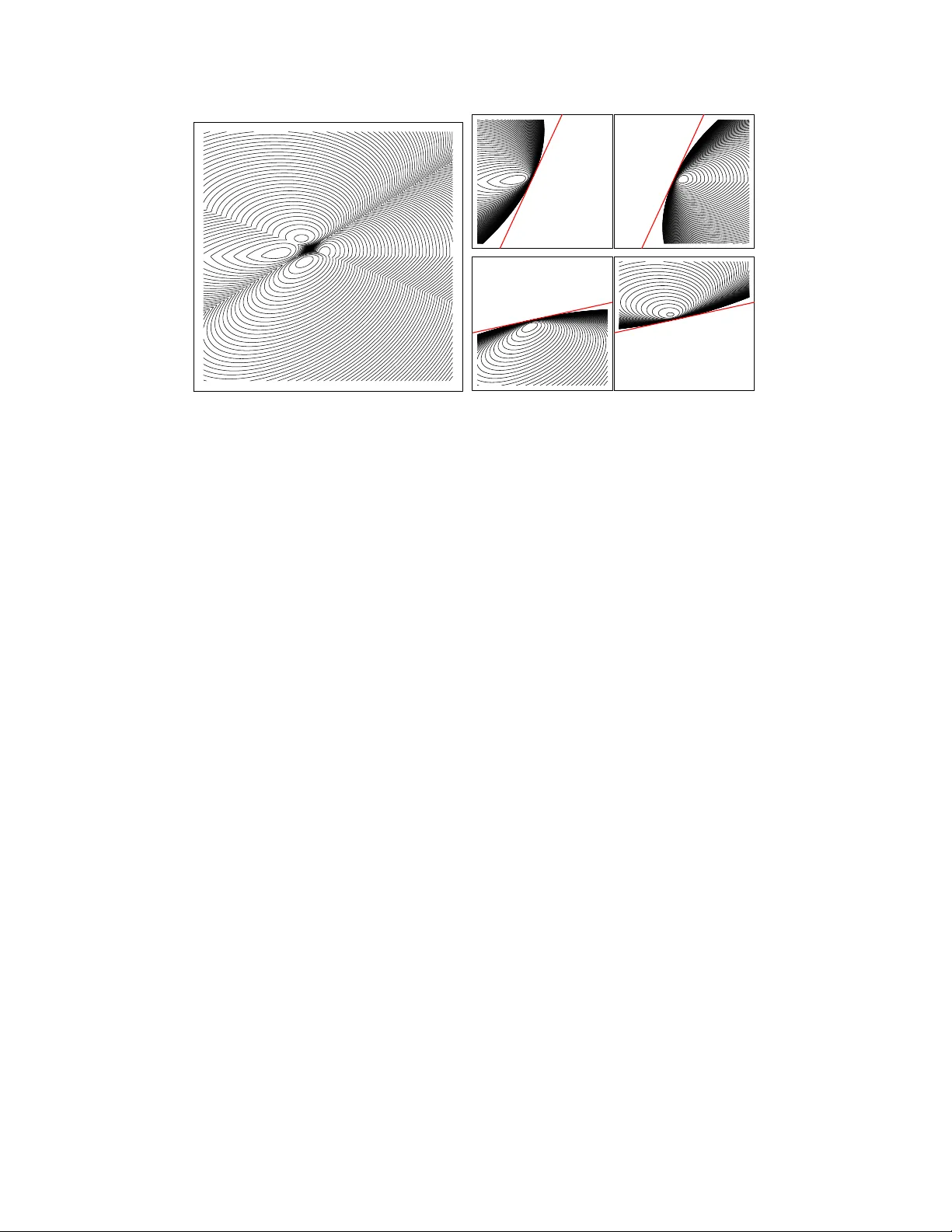
Non-con v ex Global Minimization and F alse Disco v ery Rate Con trol for the TREX Jacob Bien Departmen t of Biological Statistics and Computational Biology Departmen t of Statistical Science, Cornell Univ ersit y Irina Ga ynano v a Departmen t of Statistics, T exas A&M Univ ersit y Johannes Lederer Departmen ts of Statistics and Biostatistics, Univ ersit y of W ashington, Seattle Christian L. M ¨ uller Simons Cen ter for Data Analysis, Simons F oundation Septem b er 22, 2016 Abstract The TREX is a recen tly introduced metho d for p erforming sparse high-dimensional regression. Despite its statistical promise as an alternativ e to the lasso, square-ro ot lasso, and scaled lasso, the TREX is computationally c hallenging in that it requires solving a non-con vex optimization problem. This pap er shows a remark able result: despite the non-con v exity of the TREX problem, there exists a polynomial-time algo- rithm that is guaran teed to find the global minim um . This result adds the TREX to a v ery short list of non-conv ex optimization problems that can b e globally opti- mized (principal comp onents analysis b eing a famous example). After deriving and dev eloping this new approach, w e demonstrate that (i) the ability of the preexisting TREX heuristic to reac h the global minim um is strongly dep enden t on the difficulty of the underlying statistical problem, (ii) the new p olynomial-time algorithm for TREX p ermits a no vel v ariable ranking and selection sc heme, (iii) this sc heme can b e incor- p orated in to a rule that con trols the false disco very rate (FDR) of included features in the mo del. T o achiev e this last aim, we pro vide an extension of the results of Barb er & Candes (2015) to establish that the kno ckoff filter framew ork can be applied to the TREX. This inv estigation thus provides b oth a rare case study of a heuristic for non-con vex optimization and a nov el wa y of exploiting non-conv exit y for statistical inference. Keywor ds: high-dimensional, global optimization, mo del selection, sparsit y , tuning param- eter 1 1 In tro duction The lasso (Tibshirani 1996) has b ecome a canonical approach to v ariable selection and predictiv e mo deling in high-dimensional regression settings. Giv en a matrix of features X ∈ R n × p and a resp onse v ector Y ∈ R n , the lasso is based on solving the regularized least-squares problem, min β ∈ R p  k Y − X β k 2 2 + λ k β k 1  , where λ ≥ 0 is a tuning parameter that controls the sparsit y of the solution. When Y = X β ∗ + σ ε with eac h ε i ha ving zero mean and v ariance 1, it has b een sho wn that the lasso has strong p erformance guaran tees in terms of supp ort reco very , estimation, and predictiv e p erformance if one tak es λ ∼ σ k X > ε k ∞ . T o address the problem of σ b eing t ypically unknown, Belloni et al. (2011), Sun & Zhang (2012) prop osed mo difications of the lasso ob jective function. One can view these mo difications as scaling the lasso ob jective function b y an estimate of σ, see Lederer & M ¨ uller (2015): min β ∈ R p ( k Y − X β k 2 2 1 √ n k Y − X β k 2 + γ k β k 1 ) . In this w ay , the optimal tuning parameter γ does not dep end on σ . Ho wev er, since ε and its distribution are also unkno wn in practice, Lederer & M¨ uller (2015) prop osed the TREX, whic h tak es the ab o ve argumen t one step further. Recalling that a theoretically desirable tuning parameter for the lasso is λ ∼ σ k X > ε k ∞ , they prop ose to scale the lasso ob jective b y an estimate of this quan tit y: min β ∈ R p  k Y − X β k 2 2 k X > ( Y − X β ) k ∞ + φ k β k 1  . (1) The parameter φ ≥ 0, they argue, can b e thought of as constant ( φ = 1 / 2 b eing the standard choice). They presen t sev eral promising examples in which TREX, with no tuning of φ , can b e effectively used as an alternative to the lasso. There is, ho wev er, a ma jor tec hnical difficult y in tro duced in the TREX formulation. Unlik e the lasso, square-ro ot lasso, and scaled lasso, the TREX is based on a non-conv ex optimization problem. The left panel of Figure 1 sho ws the contours of the ob jective func- tion in (1) for a simple example in whic h p = 2, revealing a complicated, non-differentiable ob jective surface with multiple lo cal minima. 2 Estimators based on non-con v ex problems can generally not b e computed. Hence, one m ust t ypically b e satisfied with either (a) a theoretical estimator that is of limited practical v alue or (b) a redefinition of the estimator as the output of a particular algorithm chosen to appro ximately (or so one hop es) optimize the ob jective function. It is rare, but fortunate, when a particular non-con vex problem of interest can be efficien tly solv ed (i.e., globally optimized). Principal comp onen t analysis is one of the few examples of a non-conv ex problem where global optimization is computationally tractable. The first term of the TREX optimization problem (1) is non-con v ex, and therefore, one migh t exp ect that one needs to resort to either (a) or (b) ab ov e. Indeed, Lederer & M ¨ uller (2015) go the latter route by introducing a heuristic sc heme in which the ` ∞ -norm is replaced b y an ` q -norm for some large v alue of q to yield a differentiable, though still non-con v ex, loss function (we will refer to this heuristic as q-TREX throughout). In strong con trast, w e deriv e a remark able and surprising result; namely , that the TREX problem, although non-conv ex, is amenable to p olynomial-time glob al optimization . The key to our approac h is the observ ation that problem (1) can b e equiv alen tly expressed as the minimum o v er 2 p conv ex problems. W e present this reduction in Section 2, and the remainder of the pap er exploits this reduction in several directions. It is rarely p ossible to pro vide a rigorous empirical ev aluation for heuristics of non- con v ex problems since generally the global minimum is imp ossible to attain certifiably . W e therefore view the TREX as an in teresting case study for non-con v ex heuristics in general and, in Section 3, we capitalize up on our ability to p erform global minimization to pro vide a detailed lo ok at the p erformance of the q-TREX heuristic. In particular, we find that the q-TREX heuristic’s statistical p erformance (in terms of estimation error) is in fact similar to that of the global minimizer of the TREX ob jectiv e, ev en though the estimates themselv es can b e quite differen t. This observ ation has imp or- tan t practical implications. In particular, it pro vides bac king for the use of the q-TREX heuristic. W e observ e that the q-TREX heuristic is faster to compute than our algorithm for global optimization, so observing similar statistical p erformance is encouraging since it suggests that we can use q-TREX on large-scale problems without loss in statistical p erformance. 3 In Section 4, w e sho w ho w a slight mo dification of the results of Barb er & Candes (2015) ab out the kno ckoff filter leads to tw o pro cedures for (pro v ably) controlling the FDR of features selected based on the TREX. In terestingly , the empirically more successful of these pro cedures exploits information ab out the 2 p subproblems to design a no vel v ariable ranking sc heme. Thus, while the main contribution of this pap er is centered around optimization and computation, this w ork has in teresting statistical implications as w ell. In Section 5, w e pro vide empirical corrob oration of our theoretical result that our TREX-based kno c k off filter do es in fact pro vide FDR con trol. W e also apply these new kno c koff filters on a large HIV-1 genotype/drug data set and attain promising results. 2 Main Prop osal 2.1 Reduction of TREX Problem to 2 p Conv ex Problems It is clear that the main complication with (1) and the source of the non-conv exit y is the quan tit y k X > ( Y − X β ) k ∞ in the denominator of the first term. Observ e that we ma y rewrite (1) as follo ws: P ∗ := min β ∈ R p ( k Y − X β k 2 2 max j ∈{ 1 ,...,p } φ | x > j ( Y − X β ) | + k β k 1 ) = min β ∈ R p min j ∈{ 1 ,...,p } ( k Y − X β k 2 2 φ | x > j ( Y − X β ) | + k β k 1 ) . The equality ab o ve sho ws that our problem can b e viewed as the minimization of a p oint wise minim um of p functions. Suc h a minimization problem can b e alternately expressed as finding the smallest of the p functions’ minima: P ∗ = min j ∈{ 1 ,...,p } P ∗ j , where P ∗ j = min β ∈ R p ( k Y − X β k 2 2 φ | x > j ( Y − X β ) | + k β k 1 ) . While the ab ov e problem is still non-con v ex, we show that its solution is obtainable b y solving t wo conv ex optimization problems. W e use the simple fact that if H 1 and H 2 are 4 subsets of R p with H 1 ∪ H 2 = R p , then min β ∈ R p g ( β ) = min  min β ∈ H 1 g ( β ) , min β ∈ H 2 g ( β )  . Letting H 1 = { β ∈ R p : x > j ( Y − X β ) ≥ 0 } and H 2 = { β ∈ R p : − x > j ( Y − X β ) ≥ 0 } , w e ma y write P ∗ j as the minim um of t w o separate minimization problems: min β ∈ R p ( k Y − X β k 2 2 φx > j ( Y − X β ) + k β k 1 s.t. x > j ( Y − X β ) ≥ 0 ) and min β ∈ R p ( k Y − X β k 2 2 − φx > j ( Y − X β ) + k β k 1 s.t. − x > j ( Y − X β ) ≥ 0 ) . In the ab o ve, we ha v e used the fact that | a | = a if a ≥ 0 and | a | = − a if a ≤ 0. Both of these problems are of a common form, whic h can b e expressed in terms of a nonzero vector v ∈ R n as P ∗ ( v ) := min β ∈ R p  k Y − X β k 2 2 v > ( Y − X β ) + k β k 1 s.t. v > ( Y − X β ) ≥ 0  . (2) Since the minimizer of P ∗ j m ust o ccur in one of these tw o half-spaces, we hav e that P ∗ j = min { P ∗ ( φx j ) , P ∗ ( − φx j ) } , and th us, w e ha ve shown in this section that P ∗ = min j ∈{ 1 ,...,p } s ∈{± 1 } P ∗ ( sφx j ) . The minimizer of (1) is therefore provided b y the ( j, s ) pair that attains the abov e mini- mization. See Algorithm 1 for the main algorithm, whic h we refer to as the c-TREX (short for conv ex-TREX). In the next section, w e sho w that (2) is a conv ex optimization problem that can b e readily solv ed, which therefore implies that we can globally minimize (1) by solving 2 p con vex problems. The left panel of Figure 1 shows the contours of the TREX ob jective in an example where p = 2. The right panel of Figure 1 shows the decomp osition of this non-con vex problem in to 4 (i.e., 2 p ) separate conv ex optimization problems. The lo w est of these 4 minima is the global minim um of (1). 2.2 Ho w to Solv e Eac h Con v ex Problem The first term in (2) can b e written as f ( Y − X β , v > ( Y − X β )) where f ( a, b ) = a 2 /b , defined on R × (0 , ∞ ), is a fairly well-kno wn conv ex function, sometimes referred to as 5 Algorithm 1 The c-TREX algorithm for globally optimizing the TREX problem (1). for j = 1 to p do for s ∈ {− 1 , 1 } do Solv e the SOCP (2) with v = sφx j as describ ed in Section 2.2. Let ˆ β ( j, s ) and P ∗ ( sφx j ) denote the optimal p oin t and v alue, resp ectiv ely . end for end for Let ( ˆ j , ˆ s ) = arg min ( j,s ) P ∗ ( sφx j ) Return ˆ β ( ˆ j , ˆ s ) “quadratic-o v er-linear” (Boyd & V andenberghe 2004). Since this term is the comp osition of a con vex function and an affine function, it is therefore con v ex (Bo yd & V anden b erghe 2004). F ollowing a tec hnique used in Lob o et al. (1998), w e can re-express (2) as a second- order cone program (SOCP). W e b egin b y writing (2) as min t 0 ,...,t p p X j =0 t j s.t. k Y − X β k 2 2 ≤ t 0 v > ( Y − X β ) v > ( Y − X β ) ≥ 0 | β j | ≤ t j for j = 1 , . . . , p. A few lines of algebra giv e us a SOCP formulation of (2): min t ∈ R p +1 ,β ∈ R p p X j =0 t j s.t.      2( Y − X β ) v > ( Y − X β ) − t 0      2 ≤ v > ( Y − X β ) + t 0 k e > j β k 2 ≤ t j for j = 1 , . . . , p, where e j ∈ R p denotes the j th canonical basis vector. W riting (2) in this w a y not only exhibits it as a conv ex optimization problem but also makes it clear how we can solve (2) using existing SOCP solvers. W e consider t w o solv ers in particular: ECOS (Embedded Conic Solv er, Domahidi et al. 2013), an in terior-p oin t solver, and SCS (Splitting Conic Solv er, O’Donoghue et al. 2016), a first-order solver. In our exp erience, ECOS pro duces 6 j = 1, s = 1 j = 1, s = −1 j = 2, s = 1 j = 2, s = −1 Figure 1: (Left) Con tours of the TREX problem (1) in an example with p = 2. (Righ t) The c-TREX, prop osed in this pap er, decomp oses the TREX in to 2 p conv ex optimization problems, corresp onding to 2 p half-spaces of R p . The solution to TREX is the smallest of these 2 p solutions. high-accurate solutions fairly rapidly for small- and mid-sized problems, but do es not scale w ell for large problems. By contrast, SCS can scale to m uch larger problem sizes b y pro ducing less accurate solutions. In practice, it is sometimes desirable to solv e (1) along a grid of v alues of φ . In suc h a case, SCS is conv enient since it allows for w arm-starting, whic h can greatly reduce the total amount of computational time. In particular, for eac h φ , we maintain a set of 2 p solutions to (2), ˆ β ( sφx j ) for s ∈ {± 1 } and j ∈ { 1 , . . . , p } . Since a small mo dification to φ is not exp ected to mak e a big c hange to ˆ β ( sφx j ) (for a fixed s and j pair), we can use ˆ β ( s ˜ φx j ) for some ˜ φ ≈ φ to initialize the solv er to get ˆ β ( sφx j ). 3 Empirical Study of q-TREX and c-TREX 3.1 In vestiga ting the Heuristic While heuristic strategies are frequen tly used to attack non-conv ex optimization problems, it is rare that one is able to inv estigate the success of these heuristics. In machine learning and statistics, it is common to ev aluate the resulting predictions of the heuristic and to use that as “evidence” of success. Ho wev er, a metho d generating go o d predictions does not 7 actually sa y anything about whether the heuristic is in fact successfully solving the original problem. Another common form of “evidence” is for authors to rerun their heuristic with man y random starts (leading to different lo cal minima) and to sho w that most of the time it gets to the smallest observ ed one. Again, this is not rigorous evidence of success since a metho d that consisten tly ends up in a sub-optimal lo cal minimum will misleadingly lo ok p erfect. A more principled approach that app ears in, for example, the combinatorial optimization literature is to prov e that the heuristic is guaranteed to get within some appro ximation ratio of the true solution. There is therefore typically a disconnect b etw een the motiv ating optimization problem and the metho d prop osed in practice. Since theoretical results are typically based on the original optimization problem rather than the heuristic, this disconnect leads to a gap b et ween the ideal method that comes with theoretical guarantees and the practical method that is actually used. The algorithm presented in this pap er therefore presents us with a rare opportunity to in vestig ate the p erformance of the q-TREX heuristic that was introduced in Lederer & M ¨ uller (2015). F or the empirical study , we compare the p erformance of c-TREX and q-TREX using a sim ulation scenario similar to Lederer & M ¨ uller (2015). W e generate data according to the linear mo del Y i = X > i β + ε i , i = 1 , . . . , n , with three regimes for the sample size n and the n um b er of v ariables p , ( n, p ) ∈ { (500 , 100) , (50 , 100) , (50 , 500) } .The first regime corresponds to large sample setting n > p , and the other tw o corresp ond to lo w sample setting n < p . W e set the num b er of nonzero v ariables s = 5, regression v ector β = (1 s , 0 p − s ), errors ε i ∼ N (0 , σ 2 ) with σ ∈ { 0 . 1 , 0 . 5 , 3 } , and v ector of predictors X i ∼ N (0 , Σ) with Σ ii = 1 and Σ ij = κ with κ ∈ { 0 , 0 . 3 , 0 . 6 , 0 . 9 } . W e ha ve also tried β = (0 . 2 , 0 . 4 , 0 . 6 , 0 . 8 , 1 . 0 , 0 p − s ) and obtained the same qualitativ e results. W e consider n rep = 21 replications for eac h com bination of { p, κ, σ } . W e use n starts = 21 initial v alues for β for q-TREX with β (0) 1 = 0 and β (0) i , i = 2 , ..., n starts initialized at random with 25% nonzero features. W e ha v e also tried initializing q-TREX with lasso solutions obtained via glmnet (Qian et al. 2013), but the results are nearly identical to random initializations. F or all the sim ulations, w e set TREX constan t φ = 0 . 5. 8 Figure 2: Probabilit y that q-TREX gets within 10 − 4 of the global optimal v alue as a function of num b er of random restarts. (The first starting p oint is alw a ys taken to b e the v ector of all zeros.) Figure 2 shows the empirical probability (ov er n rep = 21 replications) of q-TREX at- taining an ob jective v alue within 10 − 4 of the global minimum as a function of n umber of restarts. The q-TREX is successful at reco v ering the global minimum as long as κ and σ are not to o large. Sp ecifically , q-TREX fails to recov er global solution when κ = 0 . 9 and 9 Figure 3: Av erage run time of q-TREX and c-TREX o ver n rep = 21 replications, κ = 0 and κ = 0 . 9. consisten tly has lo w success probability when σ = 3. As exp ected, increasing the num b er of initial starting p oin ts leads to a larger probability of success, ho wev er using only one starting p oin t β (0) = 0 pro vides satisfactory p erformance for small κ and σ . 3.2 Timing Results W e compare q-TREX and c-TREX timing p erformance on a laptop with 3.1 GHz In tel Core i7 using Matlab R2015b. The timing for b oth changes significan tly with the dimension p , and is not significan tly influenced by κ or σ . In Figure 3 we present results for κ ∈ { 0 , 0 . 9 } . The execution time rep orted for q-TREX is the total time with 41 restarts; the execution time reported for c-TREX is the total time o ver 2 p problems using the ECOS solv er (Domahidi et al. 2013). The q-TREX is significantly faster than c-TREX. 3.3 Statistical P erformance W e hav e seen that q-TREX is m uch faster than c-TREX; how ever, Section 3.1 shows that q-TREX fails to achiev e the global minimization in some situations, for example when κ = 0 . 9. Here we inv estigate whether this computational discrepancy has an effect on 10 Figure 4: Average estimation error of q-TREX and c-TREX ov er n rep = 21 replications, κ = 0 and κ = 0 . 9. statistical p erformance. Sp ecifically , we compare the estimation error k ˆ β − β ∗ k 2 for q- TREX and c-TREX when κ ∈ { 0 , 0 . 9 } (Figure 4, the results for κ ∈ { 0 . 3 , 0 . 6 } are similar). The estimation error of q-TREX is on av erage the same as for c-TREX for all combinations of { p, κ, σ } . While w e of course do not usually kno w the true v alues of κ and σ in real settings, we find no evidence in terms of estimator p erformance that one should prefer the exact TREX solution ov er the q-TREX solution: If κ and σ are b oth small, the t wo metho ds result in the same computational and statistical p erformance. If either κ or σ is large, q-TREX may fail to ac hieve the global optimal v alue, ho wev er this will not affect the statistical p erformance. 3.4 T op ology of the Non-con v ex Ob jective While only the minimum of the 2 p function v alues P ∗ ( sφx j ) is returned in the c-TREX algorithm, in this section we study the distribution of these function v alues and in v es- tigate whether this can give us deep er insight into the underlying problem regime. In Figure 5 w e display histograms of the 2 p optimal v alues computed in the c-TREX algo- rithm: P ∗ ( sφx j ) for s ∈ {− 1 , 1 } and j ∈ { 1 , . . . , p } . W e repeat this in differen t problem 11 Figure 5: Histogram of 2 p function v alues of c-TREX for one mo del instance. Dia- mond mark ers corresp ond to q-TREX function v alues from 21 random restarts, ( κ, σ ) ∈ { (0 , 0 . 1); (0 . 6 , 3); (0 . 9 , 0 . 5) } . The histogram for p = 500, κ = 0 . 9, σ = 0 . 5 has an additional q-TREX mark er at 14 (data p oin t not shown). regimes and find that the shap e of the histogram of the 2 p v alues differs according to problem regime. In particular, we consider the following representativ e com binations of ( κ, σ ) ∈ { (0 , 0 . 1); (0 . 6 , 3); (0 . 9 , 0 . 5) } . W e observe three histogram shap es arising: • In the lo w κ , lo w σ setting (top ro w of Figure 5), the histogram is left-sk ew ed and the global minim um v alues are clearly separated from the rest. • In the mo derate κ , high σ setting (middle ro w), the histogram has a long left tail without clear separation b et ween the v alues (unless n is large). • In the high κ setting (b ottom ro w), the histogram is bimo dal regardless of the v alues 12 of n , p and σ . Since the estimation error of b oth q-TREX and c-TREX strongly depends on the v alues of ( κ, σ ), whic h are t ypically unknown, the ab ov e observ ations suggest that we can use the 2 p function v alues from c-TREX to distinguish “go o d” and “bad” regimes in practice. Figure 5 also sho ws the function v alues from 21 random restarts of q-TREX sup erim- p osed (in red diamonds) on the histogram of the 2 p function v alues of c-TREX. As expected from Figure 2, in low κ settings q-TREX attains the global minim um for the ma jority of starting points. In high κ settings, q-TREX ma y fail to reach the ob jectiv e v alue of c- TREX within 10 − 4 precision, with some starting p oints leading to ob jective v alues outside of the range of 2 p v alues of c-TREX (see p = 500, κ = 0 . 9 and σ = 0 . 5). Imp ortan tly , w e also observ e that in the low κ , low σ setting, the indices j of the P ∗ j = min { P ∗ ( φx j ) , P ∗ ( − φx j ) } corresp onding to the well-separated global or near-global optima coincide with the indices asso ciated with non-zero β j in the true solution. Th us, insp ection of these indices ma y giv e additional insights in to which en tries β j are p oten tially non-zero and motiv ates the use of P ∗− 1 j as a measure of v ariable imp ortance. In Section 4, w e use this in tuition to dev elop a pro cedure for false disco v ery rate con trol. 3.5 T op ology of the TREX function on gene expression data W e next consider a real-world high-dimensional problem from genomics that has b een in tro duced as a high-dimensional b enc hmark for linear regression in B ¨ uhlmann et al. (2014) and used in Lederer & M ¨ uller (2015) to show case q-TREX’s abilit y to do meaningful v ariable selection. The c-TREX allo ws us to re-examine these previous results and analyze the top ology of the TREX ob jectiv e function in practice. The design matrix X consists of p = 4088 gene expression profiles for n = 71 differen t strains of Bacillus subtilis (B. subtilis). The response Y ∈ R 71 giv es each strain’s corresp onding standardized rib oflavin (Vitamin B) log-pro duction rates. T o get a rich picture of the top ology , we solv ed the TREX problem ( φ = 0 . 5) using the q-TREX ( q = 40) with 4088 random restarts. W e compared the resulting solutions to the 2 p = 8176 c-TREX subproblems in terms of sparsity pattern and TREX function v alues. All numerical solutions ha v e b een thresholded at the lev el  t = 10 − 10 to discard “numerical” zeros. Key results are summarized in Figure 6. 13 Probability histogram TREX function values Sparsity of TREX solutions TREX function values Pr obability histogram TREX function values Sparsity of TREX solutions TREX function values Pr obability histogram TREX function values Sparsity of TREX solutions TREX function values Figure 6: T op ological prop erties of the TREX on the Rib ofla vin data. Left panel: Distri- bution of (lo cally) optimal function v alues for q-TREX (blue) and all 2 p subproblems of c-TREX; Righ t panel: Solution sparsity vs. TREX function v alue. The optimal c-TREX solution has 25 non-zero en tries (indicated b y the red arro w), the optimal q-TREX solution has 23 non-zero en tries (blue arro w). The left panel sho ws histograms of the solutions from q-TREX and c-TREX. The shape of the histogram of c-TREX function v alues sho ws the previously observ ed long left tail, t ypical for mo derate correlation in the design matrix and high v ariance. W e observ e that the histogram of q-TREX solutions is sk ew ed right with the ma jority of solutions being close to the global c-TREX solution. F or instance, 13% of all q-TREX runs are within 10 − 3 of the global minimum P ∗ , suggesting that on the order of 10 q-TREX restarts ma y suffice to get a TREX solution within this tolerance. The righ t panel of Figure 6 shows a strong relationship b et w een function v alue and sparsity of the solution, esp ecially for the c- TREX subproblems. The c-TREX global solution ˆ β c-TREX has s = 25 non-zero entries (red arro w Figure 6, right panel) compared to s = 23 non-zeros in the b est q-TREX solution ˆ β q-TREX . Insp ection of the t wo solutions reveals a core of 20 common v ariables (genes). Both solutions ac hieve similar prediction error (6 . 77 with ˆ β c-TREX and 6 . 82 with ˆ β q-TREX after least-squares refitting on the resp ectiv e s upport). When we threshold the en tries of ˆ β c-TREX and ˆ β q-TREX at the lev el  t = 10 − 4 , b oth solutions hav e identical supp ort with s = 17 non-zero entries. All estimated co efficien ts, their gene names, as well as further analysis are found in the App endix C. 14 4 Kno c k off Filtering with the TREX Our abilit y to ac hieve exact global minimization of the TREX ob jective and to insp ect the solutions of all 2 p TREX subproblems pro vides us with a w ealth of kno wledge ab out the problem structure that can b e potentially exploited in the design of nov el statistical inference sc hemes. Lederer & M ¨ uller (2015) pro vided empirical evidence that q-TREX is a competitive tuning-free v ariable selection alternative to the lasso when p > n . W e in v estigate here whether one can ac hiev e tuning-free v ariable selection with the TREX when there are at least as many observ ations n a v ailable as v ariables p . In particular, w e are interested in designing a v ariable selection scheme that con trols the false disc overy r ate (FDR), i.e., the exp ected prop ortion of false v ariables among the selected v ariables. F or this purpose, w e prop ose com bining the TREX with the kno c koff filtering frame- w ork, which is a recen tly developed approach for p erforming v ariable selection with FDR con trol in the con text of the statistical linear mo del (Barb er & Candes 2015). 4.1 Bac kground on the Kno c k off Filter The principal idea of the kno c koff filter is to create fake “kno c koff ” versions of the features and to ha ve these fabricated features compete with the real features that they mimic. More sp ecifically , the kno ck off filter pro cedure inv olv es three steps: (i) efficien tly generating an artificial data matrix ˜ X ∈ R n × p that closely matches the ov erall correlation structure of the actual data matrix X ∈ R n × p ; (ii) solving the linear mo del with the augmen ted design matrix [ X ˜ X ] ∈ R n × 2 p ; and (iii) calculating feature-sp ecific statistics (with certain prop erties) W j = W j ([ X ˜ X ] , Y ), where large v alues of W j indicate that the j th original feature is comp eting w ell against its kno ck off, providing evidence against the null that β j = 0. The artificial data matrix ˜ X ∈ R n × p is constructed so that ˜ X > ˜ X = X > X and X > ˜ X = X > X − diag { s } for some p -dimensional nonnegativ e v ector s . Increasing the elemen ts of s allows the kno c k- off v ariables in ˜ X to b e more distinct from their coun terparts in the original matrix X , 15 leading to b etter statistical p o wer. W e choose s with s j = s for all j , which corresp onds to the equi-correlated kno c koffs discussed in Barb er & Candes (2015). The construction of the artificial data ˜ X suggests that solving a linear mo del for the augmen ted data matrix [ X ˜ X ] ∈ R n × 2 p should lead to similar small v alues of ˆ β j and ˆ β j + p when v ariable j is not in the model, and different v alues of ˆ β j and ˆ β j + p when v ariable j is in the mo del (with ˆ β j b eing the larger in magnitude). This intuition is used for the construction of statistics W j with large p ositiv e v alues giving evidence against β j = 0. F or example, one can use W j = | ˆ β LS j | − | ˆ β LS j + p | , where ˆ β LS is the least-squares estimator. Ho w ever, many other c hoices are p ossible in combination with different v ariable selection pro cedures. F or the lasso pro cedure, a natural choice (the default lassoSignedMax setting in the published soft ware pac k age Barber et al. 2015) is defined as follo ws: Let Z j = sup { λ : ˆ β j ( λ ) 6 = 0 } for j = 1 , . . . , 2 p with ˆ β j ( λ ) b eing the solution of the lasso for a giv en λ v alue on the augmented problem regressing Y on [ X ˜ X ], then set W j = max( Z j , Z j + p ) sign( Z j − Z j + p ). 4.2 Prop osed TREX-based Kno c koff Statistics Using this in tuition, w e next in tro duce t wo no vel knock off statistics that can be used in com bination with the TREX. Our first proposal is a statistic similar to lassoSignedMax , in whic h we in tro duce a “path” version of the TREX where the scalar φ in (1) is v aried from high to lo w v alues. W e measure the quan tit y Z φ j = sup { φ : ˆ β j ( φ ) 6 = 0 } for j = 1 , . . . , 2 p where ˆ β j ( φ ) is the solution of the TREX for a giv en φ v alue on the augmen ted problem. The asso ciated statistic is W φ j = max( Z φ j , Z φ j + p ) sign( Z φ j − Z φ j + p ). A second more natural statistic is derived from the collection of 2 p function v alues of c-TREX with standard v alue φ = 0 . 5. Recall that we hav e asso ciated for eac h v ariable index j the solution P ∗ j = min { P ∗ ( φx j ) , P ∗ ( − φx j ) } . W e observ e in Section 3.4 that the indices j of (near- )optimal P ∗ j corresp ond to the indices of non-zero β j in the true solution. W e thus prop ose the function-v alue asso ciated TREX measure Z f j = P ∗− 1 j with asso ciated kno c koff statistic W f j = max( Z f j , Z f j + p ) sign( Z f j − Z f j + p ). This statistic th us tak es full adv antage of the entire top ology of the non-conv ex TREX function on the augmented problem. 16 4.3 Theoretical Justification Barb er & Candes (2015, Theorems 1 and 2) show that applying a data-dependent threshold to statistics W j leads to prov able FDR con trol assuming these statistics satisfy t wo proper- ties: antisymmetry and sufficiency (see Definitions 3 and 4 in Barb er & Candes 2015). The an tisymmetry prop erty states that sw apping X j and ˜ X j for any j ∈ { 1 , ..., p } has the effect of changing the sign of the j th statistic. The TREX-based statistics W φ = ( W φ 1 , ..., W φ p ) and W f = ( W f 1 , ..., W f p ) satisfy this prop ert y by construction as sign( W φ j ) = sign( Z φ j − Z φ j + p ) and sign( W f j ) = sign( Z f j − Z f j + p ). The sufficiency prop ert y states that the statistic only dep ends on the Gram matrix [ X ˜ X ] > [ X ˜ X ] and on the feature resp onse inner pro ducts [ X ˜ X ] > Y . Unfortunately , this prop ert y do es not hold for the TREX-based statistics due to an additional dep endence on k Y k 2 . How ever, w e show in what follo ws that the results in Barb er & Candes (2015), sp ecifically Theorems 1 and 2, hold true also under a relaxed version of the sufficiency prop ert y , whic h w e define b elow (and, imp ortan tly , this prop erty is satisfied by the statistics W φ and W f for the TREX as sho wn in Lemma A.1 in the App endix). Definition 4.1. A statistic W is said to ob ey the generalized sufficiency property if W dep ends on ( X , ˜ X , Y ) only thr ough the Gr am matrix [ X ˜ X ] > [ X ˜ X ] , the fe atur e r esp onse inner pr o ducts [ X ˜ X ] > Y , and the norm of the r esp onse ve ctor k Y k 2 , that is, W = f ([ X ˜ X ] > [ X ˜ X ] , [ X ˜ X ] > Y , k Y k 2 ) . W e call this the “generalized sufficiency prop erty” since Barb er & Candes (2015)’s sufficiency prop erty is included as a sp ecial case. The follo wing theorem is the extension of Barb er & Candes (2015)’s Theorem 1 to this more general setting. Theorem 4.1. L et W satisfy the antisymmetry and gener alize d sufficiency pr op erties de- fine d ab ove. F or any FDR tar get q ∈ [0 , 1] , define a data-dep endent thr eshold T as T = min  t ∈ W : # { j : W j ≤ − t } max(# { j : W j ≥ t } , 1) ≤ q  , and chosen mo del ˆ S = { j : W j ≥ T } . Her e, W = {| W j | : j = 1 , . . . , p } \ { 0 } is the set of unique non-zer o absolute values of the elements of W . Then, E " # { j : β j = 0 and j ∈ ˆ S } # { j : j ∈ ˆ S } + q − 1 # ≤ q . 17 Homoscedastic Heteroscedastic TP rate Correlated Empirical FDR TP rate n=101 Nominal q FDR Empirical FDR Nominal q FDR Empirical FDR Nominal q FDR Empirical FDR n=111 n=150 Figure 7: Mean and standard error of empirical FDR vs. nominal FDR level q FDR , mean TP rates vs. empirical FDR under homoscedastic ( σ = 1) (left panel) and heteroscedastic noise ( σ 1 = 0 . 7) (central panels), and correlated noise (righ t panels) for sample sizes n ∈ { 101 , 111 , 150 } across all recorded FDR levels q FDR o v er 51 rep etitions for TREX statistics W f (red) and W φ (blue), and lasso-based statistic W ( lassoSignedMax ) (y ellow). The pro of of Theorem 4.1 is deferred to App endix B. This theorem pro vides theoretical supp ort for the FDR con trol of the tw o prop osed TREX-based kno c koff filters. While our goal of course is to establish FDR con trol of the TREX kno c koff filters, it should b e noted that this new result also establishes FDR control for the square-ro ot lasso (Belloni et al. 2011), which does not satisfy the sufficiency prop ert y but do es satisfy the generalized sufficiency prop ert y . 5 Exp erimen ts with TREX-based Kno c k off Filtering 5.1 Empirical V alidation of TREX Kno c k off Pro cedures In the previous section, we prop osed t w o TREX-based knock off filters and pro ved that they pro vide FDR control. T o corrob orate these results empirically , we follow the exp erimen tal setup in Barb er & Candes (2015) and simulate syn thetic data according to the linear 18 mo del Y i = X > i β + ε i , i = 1 , . . . , n with p = 100, s = 30 nonzero v ariables, regression v ector β = 3 . 5(1 T s , 0 T p − s ) T , and feature vectors X j ∼ N (0 , Σ) with Σ j j = 1, j = 1 , . . . , p and Σ j k = κ for j 6 = k with κ = 0 . 3. W e consider three noise scenarios: homoscedastic noise with errors ε i ∼ N (0 , σ 2 ) with σ = 1, heteroscedastic noise with errors uniformly dra wn from either ε i ∼ N (0 , σ 2 1 ) or ε i ∼ N (0 , σ 2 2 ) with σ 1 = 0 . 7 and σ 2 2 = 2 − σ 2 1 , and correlated noise with ε i ∼ N (0 , Σ  ) with Σ  ha ving the same structure as Σ. Each column X j is centered and normalized. W e v ary the sample size n ∈ { 101 , 111 , 150 } and record the n umber of true p ositiv es (TPs) and the empirical FDR at nominal levels q FDR = { 0 . 05 , 0 . 1 , . . . , 0 . 95 } for r = 51 rep etitions. W e ran c-TREX with φ = 0 . 5 for the W f statistic and q-TREX o ver the φ -path φ ∈ { 0 . 1 , 0 . 15 , . . . , 1 . 45 , 1 . 5 } for W φ . W e show empirical FDR and TP results when using the TREX kno ck off filtering with statistics W f , W φ , and lasso-based kno ck off filtering with W in Figure 7. Under homoscedastic noise, w e observ e that b oth nov el statistics ob ey the nominal FDR at comparable p ow er across most samples sizes and nominal lev els. F or the lo west p ossible sample size ( n = 101), only the W f statistic ob eys the nominal FDR under all noise scenarios. Under heteroscedastic and correlated noise, the W f statistic has consistently higher TP rate than the other statistics for sample size n = 101. F or larger sample size, all statistics hav e similar p o wer at comparable empirical FDR with W f b eing the most conserv ativ e. 5.2 An Application to HIV-1 Data W e next apply TREX knock off filtering to the task of inferring mutations in the Human Imm uno deficiency Virus T yp e 1 (HIV-1) that are asso ciated with drug resistance. The original data set (Rhee et al. 2006) comprises drug resistance measurements and genot yp e information from samples of HIV-1 proteins. Separate data sets are av ailable for resistance to six protease inhibitors (PIs), to six n ucleoside reverse-transcriptase (R T) inhibitors (NR- TIs), and to three non-nucleoside R T inhibitors (NNR TIs), respectively . The sample size of the different data sets ranges from n = 329 to 843 (see Figure 9 low er panel for details). F ollowing (Barb er & Candes 2015), we analyze each drug separately using statistical linear mo dels. The resp onse Y is giv en b y log-fold c hanges of measured drug resistances. The 19 W ! W ! W ! W ! W ! W ! Figure 8: Number of p ositions on target NR TI for six drugs selected by TREX kno c koff filtering with W f and W φ statistic, lasso kno c koff filtering with lassoSignedMax statistic W , and the Benjamini-Hoch b erg (BHq) metho d at target FDR q FDR = 0 . 2. The dashed horizon tal line denotes the total num b er of p ositions in the TSM list. Data dimensions n and p for eac h exp erimen t can b e found in the lo wer panel of Figure 9. design matrix X with en tries X ij ∈ { 0 , 1 } indicates absence or presence of (at least tw o) m utations at the j th genot yp ed p osition in the R T or protease, where distinct mutations at the same p osition are treated as additional separate features. In the absence of a ground truth for this real-w orld data set, w e follo w (Barber & Cand es 2015) and compare the list of inferred mutations using kno c koff filtering with lists of treatment-selected m utation (TSM) panels (Rhee et al. 2006). These TSM lists comprise all m utations that are presen t at significan tly higher frequency in virus samples from previously treated patients compared 20 W ! W ! W ! W ! W ! W ! W ! Figure 9: Num b er of p ositions on target PI for six drugs selected b y TREX kno c koff filtering with W f and W φ statistic, lasso kno c koff filtering with lassoSignedMax statistic W , and the Benjamini-Ho c hberg (BHq) metho d at target FDR q FDR = 0 . 2. The dashed horizon tal line denotes the total n umber of p ositions in the TSM list. The brac k et marks the t wo TREX-based statistics. The low er panel sho ws the dimensionality of eac h problem. with un treated control groups. Although these lists are target (R T, NR TI, NNR TI) but not drug sp ecific, they still serv e as a helpful proxy to the set of true p ositives across all tested drugs. W e here apply TREX knock off filtering with W f and W φ statistic, lasso kno c koff filtering with lassoSignedMax statistic W , and the Benjamini-Ho ch b erg (BHq) pro cedure (Benjamini & Ho c hberg 1995) for target FDR q FDR = 0 . 2. Figure 8 summarizes the TSM recov ery performance of all metho ds for m utations in 21 NR TI across all six drugs. W e observe sev eral differences among the metho ds. First, the TREX with W f statistic selects only mutations from the TSM list across all drugs (except one additional for D4T). F or x3TC and TDF it selects one or no m utation (iden tical to the p erformance of the lasso). The TREX shows remark able p erformance for AZT (the first successful NR TI drug) where it reco vers 19 out of 24 mutations without rep orting an y m utation outside the TSM list. Using TREX with selection along the φ -path and W φ results in a less conserv ativ e v ariable selection pro cedure. Moreov er, it compares fav orably to its lasso analog with increased p ow er on TDF, x3TC, and DDI. The BHq and TREX with W φ are the only metho ds that select mutations for the drug TDF. W e next analyze TSM reco very p erformance of all metho ds for m utations in PI across sev en tested drugs (see Figure 9). W e observ e a similar trend as in the NR TI example. TREX Kno c k off filtering with W f reco v ers mostly v ariables from the TSM list at similar p o wer compared to all other methods. The p erformance of the TREX with W φ statistic is again comparable to kno c koff filtering with the lasso. Finally , on the NNR TI test case (data not shown) all metho ds show similar v ariable selection b eha vior with ab out one half of the predictions presen t in the TSM lists with additional nov el mutational p ositions. 6 Discussion In this pap er, we in tro duce a new algorithm, called c-TREX, that is guaranteed to at- tain the global minim um of the non-conv ex TREX problem. Having access to the true global minim um is extremely rare in non-conv ex optimization. W e use this new ability to inv estigate the p erformance of a previously proposed heuristic, the q-TREX, in a w ay that is typically imp ossible in other non-con v ex problems. W e observe that q-TREX’s suc- cess in attaining the global minim um is affected by v arious parameters of the underlying mo del suc h as the error v ariance and the correlation betw een features. W e do, how ever, observ e that in terms of statistical p erformance the c-TREX and q-TREX estimators are on par, suggesting that q-TREX’s sub-optimality in terms of the TREX ob jective may not negativ ely affect its p erformance as an estimator. The c-TREX algorithm in v olves solving 2 p separate con vex problems that are based on the original TREX problem. The conv ex problems b elong to the class of second-order 22 cone programs (SOCPs). W e ha v e used t wo state-of-the-art SOCP solvers: ECOS (Em- b edded Conic Solver, Domahidi et al. 2013), an interior-point solv er, and SCS (Splitting Conic Solv er, O’Donoghue et al. 2016), a first-order metho d. Our empirical in vestigations sho w that these solv ers are able to solv e c-TREX within reasonable time but are not yet comp etitiv e with the q-TREX heuristic. An in teresting line of future research is thus to design dedicated SOCP solvers that use the sp ecial structure of the TREX problem as well as pro ximal algorithms (Com b ettes & M ¨ uller 2016). Our analysis of the TREX problem landscap e shows that having access to all 2 p TREX solutions is a ric h source for insigh t ab out the underlying mo del. W e observ e that the “top ology” of these solutions app ears to differ in an informative wa y dep ending on the problem regime. W e observe that (i) the distribution of 2 p function v alues asso ciated with the solutions b ecomes increasingly multi-modal with statistical problem difficulty and (ii) the 2 p function v alues p ermit a nov el ranking sc heme for v ariable imp ortance. Another ma jor contribution of this work is that we show that the kno c k off filter can b e applied to the TREX, leading to tw o new pro cedures for con trolling the FDR for v ariable selection. One of our kno ck off statistics that p erforms particularly w ell makes explicit use of the 2 p solutions computed in the c-TREX algorithm. Our empirical study corrob orates that FDR is controlled at the nominal lev el and offers promising evidence on synthetic and real-w orld data that a strong abilit y to detect true p ositiv es is maintained. ONLINE MA TERIAL MA TLAB-pac k age for TREX routine: github.com/m uellsen/TREX References Bar, H. Y., Bo oth, J. G. & W ells, M. T. (2015), ‘A Scalable Empirical Bay es Approac h to V ariable Selection’, 14853 , 1–26. Barb er, R. F. & Candes, E. (2015), ‘Con trolling the false discov ery rate via kno c koffs’, The A nnals of Statistics 43 (5), 2055–2085. 23 Barb er, R. F., Candes, E. & Patterson, E. (2015), ‘Kno c koff filter for matlab’, http: //web.stanford.edu/ ~ candes/Knockoffs/package_matlab.html . Belloni, A., Chernozh uko v, V. & W ang, L. (2011), ‘Square-ro ot lasso: pivotal recov ery of sparse signals via conic programming’, Biometrika 98 (4), 791–806. Benjamini, Y. & Ho c h b erg, Y. (1995), ‘Con trolling the false discov ery rate: a practical and p ow erful approac h to m ultiple testing’, Journal of the R oyal Statistic al So ciety B 57 (1), 289–300. Bo yd, S. & V andenberghe, L. (2004), Convex Optimization , Cambridge Universit y Press. B ¨ uhlmann, P ., Kalisch, M. & Meier, L. (2014), ‘High-Dimensional Statistics with a View T o- w ard Applications in Biology’, A nnual R eview of Statistics and Its Applic ation 1 (1), 255– 278. Com b ettes, P . L. & M ¨ uller, C. L. (2016), ‘Perspective F unctions: Prop erties, Proximal Calculus, and Applications in High-Dimensional Statistics’, arXiv pr eprint pp. 1–27. Domahidi, A., Ch u, E. & Boyd, S. (2013), ECOS: An SOCP solver for em b edded systems, in ‘Europ ean Control Conference (ECC)’, pp. 3071–3076. Lederer, J. & M ¨ uller, C. (2015), Don’t fall for tuning parameters: T uning-free v ariable selection in high dimensions with the trex, in ‘Pro ceedings of the Tw ent y-Ninth AAAI Conference on Artificial In telligence’. Lob o, M. S., V andenberghe, L., Bo yd, S. & Lebret, H. (1998), ‘Applications of second-order cone programming’, Line ar algebr a and its applic ations 284 (1), 193–228. O’Donogh ue, B., Chu, E., Parikh, N. & Bo yd, S. (2016), ‘Conic optimization via op erator splitting and homogeneous self-dual em b edding’, Journal of Optimization The ory and Applic ations, to app e ar . Qian, J., Hastie, T., F riedman, J., Tibshirani, R. & Simon, N. (2013), ‘Glmnet for matlab’, http://www.stanford.edu/ ~ hastie/glmnet_matlab/ . 24 Rhee, S.-Y., T aylor, J., W adhera, G., Ben-Hur, A., Brutlag, D. L. & Shafer, R. W. (2006), ‘Genot ypic predictors of h uman immunodeficiency virus t yp e 1 drug resistance’, Pr o c e e d- ings of the National A c ademy of Scienc es 103 (46), 17355–17360. Sun, T. & Zhang, C.-H. (2012), ‘Scaled sparse linear regression’, Biometrika 99 (4), 879–898. Tibshirani, R. (1996), ‘Regression shrink age and selection via the lasso’, Journal of the R oyal Statistic al So ciety B pp. 267–288. APPENDIX A Generalized Sufficiency Prop ert y of W φ and W f Lemma A.1. The statistics W φ and W f c an b e written as W φ = g φ  [ X ˜ X ] > [ X ˜ X ] , [ X ˜ X ] > Y , k Y k 2  and W f = g f  [ X ˜ X ] > [ X ˜ X ] , [ X ˜ X ] > Y , k Y k 2  for some g φ : S + 2 p × R 2 p × R → R p and g f : S + 2 p × R 2 p × R → R p , wher e S + 2 p is the c one of 2 p × 2 p p ositive semidefinite matric es. Pr o of. The TREX criterion (1) can b e rewritten as min β ∈ R p  k Y k 2 2 − 2 β > X > Y + β > X > X β k X > Y − X > X β k ∞ + φ k β k 1  , where the ob jectiv e function dep ends on the data only through X > X , X > Y , and k Y k 2 . By construction, this is also true for each conv ex subproblem (2). B Pro of of Theorem 4.1 Lemma B.1. Ther e exists an ortho gonal matrix R ∈ R n × n such that R [ X ˜ X ] = [ X ˜ X ] swap( S ) . Pr o of of L emma B.1. Define the square matrix M := [ X ˜ X ] swap( S ) [ X ˜ X ] > , and consider its full singular v alue decomp osition M = U m D m V > m , with D m b eing a square diagonal matrix 25 of singular v alues. W e show that an orthogonal matrix R = U m V > m satisfies the conditions of the lemma: R [ X ˜ X ] − [ X ˜ X ] swap( S ) = 0. Consider the F rob enius norm k R [ X ˜ X ] − [ X ˜ X ] swap( S ) k 2 F = trace  [ X ˜ X ] > R > R [ X ˜ X ] + [ X ˜ X ] > swap( S ) [ X ˜ X ] swap( S ) − 2 R > [ X ˜ X ] swap( S ) [ X ˜ X ] >  = trace(2[ X ˜ X ] > [ X ˜ X ] − 2 V m U > m U m D m V > m ) = trace(2[ X ˜ X ] > [ X ˜ X ] − 2 D m ) , where in the second equation we used the definition of R , and the in v ariance of the Gram matrix [ X ˜ X ] > [ X ˜ X ] under the sw ap( S ) op eration. F rom the ab ov e displa y , the F rob enius norm is zero iff trace([ X ˜ X ] > [ X ˜ X ]) = trace( D m ). W e conclude the pro of by showing that the latter inequalit y holds. Consider the full singular v alue decomp osition of [ X ˜ X ] = U x D x V > x . Using the definition of matrix M , and the inv ariance of Gram matrix [ X ˜ X ] > [ X ˜ X ] under the swap( S ) op eration, M > M = [ X ˜ X ][ X ˜ X ] > swap( S ) [ X ˜ X ] swap( S ) [ X ˜ X ] > = [ X ˜ X ][ X ˜ X ] > [ X ˜ X ][ X ˜ X ] > = U x D x V > x V x D x U > x U x D x V > x V x D x U > x = U x D 4 x U > x . On the other hand, using the full singular v alue decomp osition of M , M > M = V m D 2 m V > m . It follows that V m D 2 m V > m = U x D 4 x U x , and b oth equations can b e view ed as eigendecomp o- sition of M > M . Hence, D 4 x = D 2 m up to the p erm utation, and subsequently trace( D m ) = trace( D 2 x ). Since trace([ X ˜ X ] > [ X ˜ X ]) = trace( D 2 x ) = trace( D m ), this concludes the pro of. Pr o of of The or em 4.1. In Barb er & Candes (2015), the sufficiency prop ert y is only used in the pro of of Lemma 1, where it is sho wn that for any subset S of null features N = { j ∈ { 1 , . . . , p } : β j = 0 } , W swap( S ) d = W , 26 where d = means equalit y in distribution and sw ap( S ) swaps the columns X j and ˜ X j in [ X ˜ X ] for eac h j ∈ S . F urther we show that this also holds for generalized sufficiency prop ert y . By Lemma B.1, there exists an orthogonal matrix R ∈ R n × n suc h that R [ X ˜ X ] = [ X ˜ X ] swap( S ) . (3) Therefore, W swap( S ) = f ([ X ˜ X ] > swap( S ) [ X ˜ X ] swap( S ) , [ X ˜ X ] > swap( S ) Y , k Y k 2 ) = f ([ X ˜ X ] > [ X ˜ X ] , [ X ˜ X ] > R > Y , k R > Y k 2 ) = f ([ X ˜ X ] > [ X ˜ X ] , [ X ˜ X ] > Y 0 , k Y 0 k 2 ) with Y 0 := R > Y . Hence, W swap( S ) can be viewed as W applied to the same [ X ˜ X ] and mo dified resp onse Y 0 . Since [ X ˜ X ] is fixed, it follo ws from ab o ve that to sho w W swap( S ) d = W , it is sufficien t to sho w Y d = Y 0 . Since Y ∼ N ( X β , σ 2 I ), Y 0 = R > Y ∼ N ( R > X β , σ 2 R > R ) = N ( R > X β , σ 2 I ) , where w e used the orthogonality of matrix R . F rom ab ov e, to show Y d = Y 0 , it remains to sho w R > X β = X β . Denote [ X ˜ X ] swap( S ) = [ X swap( S ) ˜ X swap( S ) ]. Since S only contains n ull features, X β = X swap( S ) β , hence R > X β = R > X swap( S ) β . On the other hand, (3) implies RX = X swap( S ) . Performing left m ultiplication b y R > on b oth sides giv es X = R > X swap( S ) , and subsequently X β = R > X swap( S ) β . Combining this with the ab o ve display gives R > X β = X β completing the pro of. C F urther analysis of TREX on the B. subtilis data This section pro vides additional information ab out the solution qualit y of the c-TREX globally optimal and the q-TREX solution. Figure 10 sho ws k ey results. W e first rep ort the correlation structure of the selected features for the q-TREX and c-TREX solutions, 27 along with the corresp onding B. subtilis gene names. W e observe tw o blo cks of correlated genes: the set XHLB, XKDS, XL Y A, and XTRA, and the pair YDDK, YDDM, (Figure 10, top panels), suggesting that the set of genes might b e further reducible, e.g., via empirical Ba y es approaches (Bar et al. 2015). W e also sho w least-squares refits on the supp ort of the q-TREX and c-TREX solution to the measured log-pro duction rate (Figure 10, low er left panel). q- TREX c- TREX MAE 0.2466 0.2466 AIC 33.91 37.47 Solutions ranked by function value Solution sparsity Figure 10: T op panels: Correlation matrix of the features (genes) selected b y q-TREX (left panel) and c-TREX (right panel); Low er left panel: Fitted log-pro duction rate vs. measured rib oflavin log-pro duction rate. The table insert shows the mean absolute error (MAE) and the Ak aike Information Criterion (AIC) for the q-TREX and c-TREX solutions; Lo w er right panel: Sparsity of all q-TREX restart solutions and c-TREX subproblems vs. ranking of the solution in terms of TREX function v alue. 28 While b oth solutions yield similar mean absolute error (MAE), the AIC of the q-TREX compares fa v orably to that of the c-TREX global minimum due to lo wer model complexity . In terms of AIC, b oth solutions impro v e up on solutions found b y Lasso with stability selection (B¨ uhlmann et al. 2014) and an empirical Ba yes approac h (Bar et al. 2015) and are comparable in terms of MAE. F or completeness, w e also rep ort the sparsity of all found solutions vs. their ranking in terms of function v alues (Figure 10, low er right panel). W e observ e that more than the top 20% of the q-TREX solutions hav e sparsity s = 23 whereas the sparsit y of the top 20% of the c-TREX solutions v ary b etw een 18 and 40. 29