Stabilizability of Markov jump linear systems modeling wireless networked control scenarios (extended version)

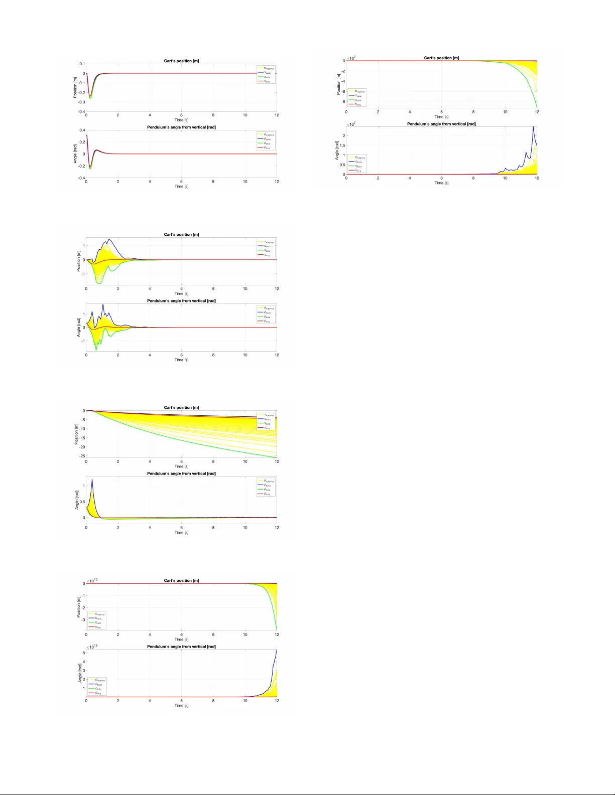
Stabilizability of Marko v jump linear systems modeling wir eless network ed control scenarios Y uriy Zacchia Lun and Alessandro D’Innocenzo Abstract — The communication channels used to conv ey infor - mation between the components of wireless network ed control systems (WNCSs) are subject to packet losses due to time- varying fading and interference. The WNCSs with missing packets can be modeled as Mark ov jump linear systems with one time-step delayed mode observ ations. While the problem of the optimal linear quadratic regulation f or such systems has been already solved, we derive the necessary and suf- ficient conditions for stabilizability . W e also show , with an example considering a communication channel model based on WirelessHAR T (a on-the-market wireless communication standard specifically designed for process automation), that such conditions are essential to the analysis of WNCSs where packet losses are modeled with Bernoulli random variables repr esenting the expected value of the real random process gover ning the channel. I . I N T RO D U C T I O N From the automatic control perspectiv e, the wireless com- munication channels are the means to con ve y informa- tion between sensors, actuators, and computational units of wireless networked control systems. These communication channels are frequently subject to time-varying fading and interference, which may lead to packet losses. In the wireless networked control system (WNCS) lit- erature the packet dropouts have been modeled either as stochastic or deterministic phenomena [1]. The proposed deterministic models specify packet losses in terms of time av erages or in terms of worst case bounds on the number of consecuti ve dropouts (see e.g. [2]). For what concerns stochastic models, a vast amount of research assumes mem- oryless packet drops, so that dropouts are realizations of a Bernoulli process ([3], [4], [5]). Other works consider more general correlated (b ursty) packet losses and use a transition probability matrix (TPM) of a finite-state stationary Markov chain (MC, see e.g. the finite-state Markov modelling of Rayleigh, Rician and Nakagami fading channels in [6] and references therein) to describe the stochastic process that rules packet dropouts (see [3], [7], [8]). In these works networked control systems with missing packets are modeled as time-homogeneous Markov jump linear systems (MJLSs, [9]), with one time-step delayed mode observations. Y . Zacchia Lun is with the IMT School for Advanced Studies Lucca, Italy . A. D’Innocenzo is with the Department of Information Engineering, Computer Science and Mathematics of the University of L ’Aquila, Italy . The research leading to these results has receiv ed funding from the Sofidel SpA and T uscan y Region under POR FSE 2014-2020, Priority Axis A - Action A.2.1.7 - project SINCERA, number 172847, CUP D61J17000000004, and from the Italian Gov ernment under CIPE resolution n.135 (Dec. 21, 2012), project INnovating City Planning thr ough Information and Communication T echnologies (INCIPICT). While the problem of the optimal linear quadratic regu- lation for such systems has been apparently solved [8], the existing solution does not consider the aspects of stabiliz- ability . As the main contribution of this article we derive the necessary and sufficient conditions for stabilizability of WNCSs modeled as MJLSs with one time-step delayed mode observ ations. In addition to this, we provide an ex- ample considering a communication channel model based on W irelessHAR T (a on-the-market wireless communication standard specifically designed for process automation) and show that the stationary MJLS model deri ved from the ac- curate Markov channel representation of the communication channel permits to discover and overcome the challenging subtleties arising from bursty behavior . W e also show that our stabilizability conditions are essential to the analysis of WNCSs that consider Bernoulli dropouts, when the Bernoulli random variables represent the expected v alue of the real random process governing the packet losses. Notation and pr eliminaries . In the following, N 0 denotes the set of non-negativ e integers, while F indicates the set of either real or complex numbers. The absolute value of a number is denoted by | · | . W e recall that every finite- dimensional normed space over F is a Banach space [10], and denote the Banach space of all bounded linear operators of Banach space X into Banach space Y , by B ( X , Y ) , and set B ( X , X ) , B ( X ) . The identity matrix of size n is indicated by I n . The operation of transposition is denoted by apostrophe, the complex conjugation by ov erbar , while the conjugate transposition is indicated by superscript ∗ , the real part of the elements of the complex matrix by < ( · ) . W e denote by ρ ( · ) the spectral radius of a square matrix (or a bounded linear operator), i.e., the lar gest absolute v alue of its eigen v alues, and by k·k either any vector norm or any matrix norm. Since for finite-dimensional linear spaces all norms are equiv alent [11, Theorem 4.27] from a topological viewpoint, as vector norms we use v ariants of vector p -norms. F or what concerns the matrix norms, we use ` 1 and ` 2 norms [12, p. 341], that treat n r × n c matrices as vectors of size n r n c , and use one of the related p -norms. The definition of ` 1 and ` 2 norms is based on the operation of vectorization of a matrix, v ec( · ) , which is further used in the definition of the operator vec 2 ( · ) , to be applied to any block matrix, e.g. Φ =  Φ ij  N i,j =1 , as if its blocks Φ ij of size n r × n c were the simple elements: v ec 2 ( Φ ) , [v ec(Φ 11 ) , . . . , vec(Φ N 1 ) , vec(Φ 12 ) , . . . , vec(Φ N N )] 0 . The linear operator v ec 2 ( · ) is a uniform homeomorphisms, its in verse operator ve c − 2 ( · ) is uniformly continuous [13], and any bounded linear operator in B  F N n r × N n c  can be represented in B  F N 2 n r n c  trough v ec 2 ( · ) . Then,  indicates the operation of matrix augmentation, i.e., the horizontal concatenation of two matrices with the same number of rows. W e denote by ⊗ the Kronecker product defined in the usual way , see e.g. [14], and by ⊕ the direct sum. Notably , the direct sum of a sequence of square matrices (Φ i ) N i =1 produces a block diagonal matrix, having its elements, Φ i , on the main diagonal blocks. Then, trace ( · ) indicates the trace of a square matrix. For two Hermitian matrices of the same dimensions, Φ 1 and Φ 2 , Φ 1  Φ 2 (respectiv ely Φ 1  Φ 2 ) means that Φ 1 − Φ 2 is positiv e semi-definite (respectiv ely positiv e definite). Finally , E ( · ) stands for the mathematical expectation of the underlying scalar v alued random variables. I I . C O M M U N I C A T I O N C H A N N E L M O D E L The challenges in analysis and co-design of WNCSs are best e xplained by considering wireless industrial control protocols. In this paper we focus on a networking protocol specifically de veloped for wireless industrial automation, i.e. W irelessHAR T [15], which is based upon the physical layer of IEEE 802.15.4-2006. Since interlea ving and forward error correction techniques appear only in the IEEE 802.15.4-2015 version of the standard, ev en one erroneous bit leads to a corrupted W irelessHAR T data packet. According to the IEEE standard [16, p. 268], the bit error ratio (BER, R b ) depends only on the signal-to-noise-plus-interference ratio (SNIR), that may be expressed by the sum of weighted log- normal processes. Such model admits an accurate log-normal approximation based on moment matching method [17]. In the follo wing we will indicate this approximation as analytic model. Notably , using a logarithmic scale for the values of SNIR, denoted by Γ , gi ves a normally distributed probability density function with mean µ and v ariance σ 2 , Γ ∼ N  µ, σ 2  . For notational con venience, we will indicate by γ the power value corresponding to SNIR Γ , i.e. Γ , 10 log 10 ( γ ) [dB]. An analytic model may be used to create a finite-state Markov channel model [6] that captures the essence of time-varying channel behavior by associating a binary sym- metric channel to each state of an er godic discrete-time MC. Clearly , the approximation becomes more accurate as the number of MC states becomes larger . Con versely , the coarsest approximation of the channel beha vior looks at only one state and may completely neglect second-order statistics. It considers the packet error probability to follo w a Bernoulli distribution. This simple model has been widely adopted in the WNCSs literature. In Section IV we will sho w that when the derived (strong) stabilizability conditions are satisfied, the linear quadratic regulation with Bernoulli dropouts [3] provides a mode-independent solution to the optimal infinite- horizon state feedback control problem over a more rigorous representation of the wireless communication channel. Here, we sho w a link between the stochastic and deterministic models by deriving worst case bounds on the number of consecutiv e dropouts. Analytic model. The reference scenario is gi ven by a certain number of coe xisting and independent W irelessHAR T networks. For simplicity , here we assume that there are only two networks, and the transmitted signals are af fected by path loss [16, p. 274], (log-normal) shadowing, and additiv e white noise introduced by the channel. Since in industrial setting highly absorbing en vironments eliminate multipath propagation [18], the multipath-induced fading is neglected. The considered modulation scheme is offset quadrature phase-shift ke ying direct-sequence spread spectrum, and it is supported by a coherent demodulation. T o conv ey the control system data, W irelessHAR T uses Publish data messages [15, p. 248], where the minimum update period is 0 . 1 s, time slot period T s is 0 . 01 s, and the frame length L F for e.g. four relev ant state variables is 26 octets. From [16, p. 268] and the absence of the forward error correction, the packet error rate (PER, R p ) is related to SNIR through BER, where γ ∈ (0 , ∞ ) , and R b ( γ ) ∈ [0 , 0 . 5] , R p ( γ ) ∈ [0 , 1] are both monotonically non-increasing: R p ( γ ) = 1 − (1 − R b ( γ )) L F , where R b ( γ ) = 1 30 16 X i =2 ( − 1) i 16 i ! e ( 20 γ 1 − i i ) . So, for L F = 208 , we have that R p < 2 . 22 · 10 − 16 ∀ γ  ≥ 3 . 882 (that is, Γ  ≥ 5 . 89 dB), and R p < 3 . 17 · 10 − 10 (i.e, a rate of less than 1 data packet lost in a year of continuous operation with the sampling time T s ) ∀ γ ? ≥ 2 . 859 (i.e., Γ ? ≥ 4 . 56 dB). Since in practical applications the probability of packet error burst of length L B is negligible when it is smaller than a specified threshold ε , which may be as small as the machine epsilon , the highest number of consecutiv e dropouts L B ( ε ) may be obtained as follows. As Γ ∼ N  µ, σ 2  , its cumulativ e distribution function F Γ ( ε ) gives the probability of a single packet loss, while F Γ ( ε ) L B is the probability of L B consecutiv e packet losses, so L B ( ε ) = ceil   ln( ε ) ln  1 2  1 + erf  Γ( ε ) − µ σ √ 2      , (1) where ceil( · ) , ln( · ) and erf ( · ) are the ceiling, natural loga- rithm, and error functions, respectively . As an illustrati ve e xample, consider ε ? = 3 . 17 · 10 − 10 , so that Γ( ε ? ) = Γ ? = 4 . 56 dB, on a wireless communication channel with ˆ µ = 10 . 15 dB and ˆ σ = 4 . 85 dB. Then, L B ( ε ? ) = 11 . For ε  = 2 . 22 · 10 − 16 and the same channel characterized by ˆ µ , ˆ σ , we have instead that Γ( ε  ) = Γ  = 5 . 89 dB, so that L B ( ε  ) = 22 . Since the probability density function f Γ ( · ) of the model is known, and R p is a continuous function defined on the range of Γ , by the law of the unconscious statistician, the e xpected value of the PER can be obtained as R + ∞ −∞ R p (10 α 10 ) f Γ ( α ) dα , and its variance can be deriv ed in a similar fashion. On the channel ˆ Γ ∼ N  ˆ µ, ˆ σ 2  having ˆ µ = 10 . 15 dB and ˆ σ = 4 . 85 dB, E (R p ( ˆ Γ)) = 0 . 008 , while the PER variance equals to 0 . 006 . Finite-state abstractions. The analytic model of a channel is defined on continuous state-space. Howe ver , there are se v- eral application scenarios (e.g. modeling channel error b ursts, decoding in channels with memory , adaptiv e transmission) where using a finite number of channel states can be more advantageous [6]. The coarsest abstraction of the analytic model collapses the infinite-dimensional state-space into one state with a representati ve PER (gi ven by its e xpected value), which may be seen as a probability of the packet loss event in the Bernoulli distribution. In more accurate finite-state Markov channel abstraction the range of SNIR is divided into se veral consecuti ve regions. A region i is mapped into a state s i of the related MC and is delimited by two thresholds α i and α i +1 . The steady state probability of the state s i is the probability that the SNIR is between the thresholds of the re- gion, i.e. p i = R α i +1 α i f Γ ( α ) dα , while the PER associated to the same state is gi ven by its e xpected v alue within the respecti ve region, that is R i p = 1 p i R α i +1 α i R p (10 α 10 ) f Γ ( α ) dα . The TPM may be then obtained by integrating the joint probability density function of the SNIR [6] over two consecuti ve packet transmissions and ov er the desired regions. In the literature on finite-state Mark ov channel abstractions there are dif ferent methods of partitioning of the range of SNIR [6], [19]. For simplicity of the presentation, in this paper we choose Γ( ε ) as the only threshold. Γ( ε ) divides the range of SNIR in two intervals. In this way we obtain a Markov channel with just two operational modes, where only one mode of operation has nonzero packet error probability . This model is known as Gilbert channel [6]. It is the easiest nontri vial example of channel models with memory . I I I . O P T I M A L C O N T RO L S C H E M E S Consider a linear stochastic system with intermittent con- trol packets due to the lossy communication channel [3] x k +1 = Ax k + B u a k + w k , with u a k = ν k u c k , (2) where, x k ∈ F n x is a system state, u a k ∈ F n u is the control input to the actuator , A and B are state and input matrices of appropriate size, respectively , u c k ∈ F n u is the desired control input computed by the controller , w k ∈ F n x is a Gaussian white process noise with zero mean and cov ariance matrix Σ w . The process noise w k is assumed to be independent from the initial state x 0 and from the stochastic v ariable ν k , which models the packet loss between the controller and the actuator: if the pack et is correctly deli vered then u a k = u c k , otherwise if it is lost then the actuator does nothing, i.e., u a k = 0 . This compensation scheme is summarized by (2). In the follo wing, we assume full state observ ation with no measurement noise, and no observation packet loss, so the optimal control must necessarily be a static state feedback and no filter is necessary . In such setting, we will compare the performance of the optimal state feedback controller under TCP-like protocols [3] (treating ν k as independent and identically distributed (i.i.d.) Bernoulli random v ariables, with information set av ailable to the controller defined as F k ,  x k , ν k − 1  , where x k = ( x t ) k t =0 , and ν k = ( ν t ) k t =0 , and optimal linear quadratic regulator for MJLS, in the presence of one time-step delayed mode observations [8], which considers ν k as a random variable governed by the Markov channel deriv ed from the model of Section II. Linear quadratic regulation with Bernoulli dropouts. The optimal state-feedback controller accounting for the i.i.d. packet losses follo wing a Bernoulli distribution, with Pr( ν k = 1) = ˆ ν for all k , minimizes the performance index J b = lim t →∞ 1 t E ( P t k =0 ( x ∗ k Qx k + u b ∗ k Ru b k ) | F k ) , where Q  0 and R  0 are the state weighting and control weighting matrices, respecti vely . The optimal controller is giv en by u b k = − ( R + B ∗ X b ∞ B ) − 1 ( B ∗ X b ∞ A ) x k = K b x k , where X b ∞ is the unique positiv e semi-definite solution of the modified algebraic Riccati equation (MARE, [3]) X b ∞ = A ∗ X b ∞ A − ˆ ν ( A ∗ X b ∞ B )( R + B ∗ X b ∞ B ) − 1 ( B ∗ X b ∞ A ) + Q . If ( A, B ) is control- lable, and ( A, Q ) is observ able, the solution X b ∞ is stabilizing if and only if ˆ ν > ν c (see [3] together with [20]), where ν c is the critical arriv al probability , that satisfies the following analytical bound: ν c ≤ p max , with p max , 1 − Π i | λ u i ( A ) | − 2 , where λ u i ( A ) are unstable eigen v alues of A . Notably , when B is rank 1 , ν c = p max . The optimal controller attains the optimal value of the performance index, i.e., J b ? = trace  X b ∞ Σ w  . MJLS with one time-step delayed mode observations. When the finite-state Marko v channel representation of the communication channel is available, to each state s i of the MC (characterising the ev olution of the channel) is associated a discrete memoryless channel. The network ed control system using such communication channel can be modelled as Markov jump system in the following manner . Consider the stochastic basis (Ω , G , ( G k ) , Pr) , where Ω is the sample space, G is the σ -algebra of (Borel) measurable ev ents, ( G k ) is the related filtration, and Pr is the probability measure. Then, the communication channel state is the output of the discrete-time MC Θ : N 0 × Ω → S defined on the probability space, that takes v alues in a finite set S , { s i } N i =1 . ∀ k ∈ N 0 the transition probability between the channel’ s states is defined as p ij = Pr { θ k +1 = s j | θ k = s i } ≥ 0 , P N j =1 p ij = 1 . The associated TPM is a stochastic N × N matrix with entries p ij , i.e.,  p ij  N i,j =1 . The probability of the successful packet deliv ery and packet loss are now conditioned to the state of the communication channel, i.e. respectively Pr( ν k = 1 | θ k = s i ) = ˆ ν i , Pr( ν k = 0 | θ k = s i ) = 1 − ˆ ν i . (3) W e observe that the networks based on IEEE 802.15.4 compatible hardware provide a SNIR estimation procedure, which is performed during link quality indicator measure- ment [16, p. 65]. The estimated v alue of the SNIR falls into one of the regions in which the range of SNIR is partitioned. In this way the corresponding state s i of the Markov channel is unequiv ocally determined, and ˆ ν i = 1 − R i p . W e present the systems in terms of the Mark ov framework [9] via the augmented state ( x k , ( θ k , ν k )) , where ν k accounts for two possible operational modes, i.e., in closed loop, when ν k = 1 , and in open loop, if ν k = 0 , while θ k describes the channel ev olution. Since the probability of a particular operational mode depends on the state of the communication channel, we denote the aggregated state ( θ k , ν k ) by ν θ k , which is a 2 N -ary random quantity . The operational modes are observ ed by controller via acknowledgements, which are a vailable only after the current decision on the gain to apply has been made and sent through the channel, because the actual success of the transmission is not known in advance. W e assume that the acknowledgments, and also the communication channel states (measured through SNIR), are not received at the controller instantaneously , but become av ailable before the next decision on the control to apply . So, we are dealing with one time-step delayed mode observations, as presented in [8], and the informational set av ailable to the controller is G k =  x k , ν k − 1 θ  , with x k = ( x t ) k t =0 , and ν k θ = ( θ t , ν t ) k t =0 . The state space representation of the system is x k +1 = Ax k + ν θ k B u k + w k , (4) where the Gaussian process noise w k (having the zero mean and cov ariance matrix Σ w ) is assumed to be independent from the initial condition ( x 0 , ν θ 0 ) and from the Markov process ν θ k for all v alues of discrete time k . W e make the assumption that the MC Θ is ergodic, with the steady state distribution p i defined as lim k →∞ Pr( θ k = s i ) , so the aggregated Marko v process ν θ k is also ergodic. The optimal mode-dependent infinite-horizon state feed- back controller is obtained from the solution of the follo wing coupled algebraic Riccati equations (CAREs), that are con- structed via the general procedure described in [8], after few manipulations that take into account the particular structure (4) of the considered MJLS: X c ∞ ,i = A i − C i B − 1 i C ∗ i , X c ∞ ,i = X c ∗ ∞ ,i  0 , (5) A i = A ∗  X N j =1 p ij X c ∞ ,j  A + Q, C i = A ∗  X N j =1 p ij ˆ ν j X c ∞ ,j  B , B i = X N j =1 p ij ˆ ν j  B ∗ X c ∞ ,j B + R  . The optimal mode-dependent state feedback controller is gi ven by u k = K c θ k − 1 x k , where K c i = B − 1 i C ∗ i . The performance inde x optimized by this controller is J c = lim sup t →∞ 1 t E ( P t k =0 ( x ∗ k Qx k + u ∗ k Ru k ) | G k ) , which, for the optimal control law , equals to J c ? = P N i =1 p i trace( X c ∞ ,i Σ w ) . Clearly , the necessary condition for the existence of the stabilizing solution X c ∞ ,i , ∀ i ≤ N , to the CAREs (5) is the (mean square) stabilizability of the system (4). Ho wev er , for the best of our knowledge, such conditions hav e not been derived yet, since e.g. the well-known stabilizability conditions of the MJLSs with the instantaneous perfect observation of the operational mode [9, pp. 57 – 58] clearly do not account for the one-step delayed observation of the channel’ s state, as will be illustrated on a numerical example in Section V. In the next subsection we derive the necessary and sufficient conditions for the mean square stabilizability of the system (4). I V . S TA B I L I Z A B I L I T Y A NA L Y S I S Consider first the system (4) without process noise, i.e., x k +1 =  A + ν θ k B K θ k − 1  x k , (6) where K θ k − 1 is a mode-dependent state-feedback controller with one time-step delayed operational mode observation, according to the informational set G k . T o account for the dependence on K θ k − 1 in the behavior of the continuous state x k , we augment the system’ s state with the memory of the pre vious state of the communication channel, i.e., the new aggregated state is ( x k , ν θ k , θ k − 1 ) , or, equiv alently , ( x k , ν k , ( θ k , θ k − 1 )) , where the last term underlines the simi- larity with the MCs with memory of order 2 , see [21] for additional details on MCs with memory . The introduced memory is, howe ver , fictitious, since the aggregated MC obeys to the Markov property of the memoryless chain Θ : Pr( θ k +1 = s j , θ k = s i | θ k 6 = s i , θ k − 1 = s ` ) = 0 , ∀ s ` ∈ S , (7) Pr ( θ k +1 = s j , θ k = s i | θ k = s i , θ k − 1 = s ` ) = Pr( θ k +1 = s j | θ k = s i ) = p ij , ∀ s ` ∈ S , (8) where the first equality in (8) is due to the fact that the inter- section of a set with itself is the set itself, so the joint prob- ability Pr( θ k = s i , θ k = s i , θ k − 1 = s ` ) = Pr( θ k = s i , θ k − 1 = s ` ) , which implies that Pr( θ k = s i | θ k = s i , θ k − 1 = s ` ) = 1 , by the definition of the conditional probability . T aken together with the chain rule of probability , the last equality implies the first equality in (8). The second equality in (8) is clearly obtained from the direct application the Markov property . The joint probability of being in an augmented Markov state ( θ k , θ k − 1 ) ev olves according to (7) and (8), so, after denoting Pr( θ k +1 = j, θ k = i ) by π ( k +1) ij , one has that π ( k +1) ij = X N ` =1 π ( k ) `i p ij . (9) The joint probability π ( k ) `i may be defined through the indi- cator function 1 { θ k = i,θ k − 1 = ` } , that indicates the membership (or non-membership) of a given element in the set, as E  1 { θ k = i,θ k − 1 = ` }  = π ( k ) `i . (10) The indicator function 1 { θ k = i,θ k − 1 = ` } allows us obtain- ing recursi ve dif ference equations for the first and second moments of the system’ s state, which are fundamental in deriving our result on stabilizability . Specifically , we define m ( k ) `i , E  x k 1 { θ k = i,θ k − 1 = ` }  , m ( k ) , h m ( k ) `i i N `,i =1 , (11) M ( k ) `i , E  x k x ∗ k 1 { θ k = i,θ k − 1 = ` }  , M ( k ) , h M ( k ) `i i N `,i =1 , (12) so that the first and second moments of x k are E ( x k ) = X N ` =1 X N i =1 m ( k ) `i , E ( x k x ∗ k ) = X N ` =1 X N i =1 M ( k ) `i . (13) Pr oposition 1: Consider the system (6). For all k ∈ N 0 , 1 ≤ `, i, j ≤ N , one has that m ( k +1) ij =  A X N ` =1 m ( k ) `i + B X N ` =1 K ` m ( k ) `i ˆ ν i  p ij , (14) M ( k +1) ij = A X N ` =1 M ( k ) `i A ∗ + B X N ` =1 K ` M ( k ) `i K ∗ ` B ∗ ˆ ν i + 2 < A X N ` =1 M ( k ) `i K ∗ ` B ∗ ˆ ν i ! ! p ij . (15) Pr oof: See Appendix. In the spirit of [9], Proposition 1 allows us to define the operators L ( · ) , [ L ij ( · )] N i,j =1 and T ( · ) , [ T `i ( · )] N `,i =1 , both in B  F N n x × N n x  , as follows. ∀ S = [S ij ] N i,j =1 , T = [T ij ] N i,j =1 , both in ∈ F N n x × N n x , we specify the inner pr oduct as h S ; T i , X N i =1 X N j =1 trace  S ∗ ij T ij  , (16) while the components of operators L ( · ) , T ( · ) , are defined by L ij ( S ) , A X N ` =1 S `i A ∗ + B X N ` =1 K ` S `i K ∗ ` B ∗ ˆ ν i + A X N ` =1 S `i K ∗ ` B ∗ ˆ ν i + B X N ` =1 K ` S `i A ∗ ˆ ν i ! p ij , (17) T `i ( S ) , A ∗ X N j =1 p ij S ij A + K ∗ ` B ∗ X N j =1 p ij S ij B K ` ˆ ν i + K ∗ ` B ∗ X N j =1 p ij S ij A ˆ ν i + A ∗ X N j =1 p ij S ij K ` ˆ ν i . (18) Remark 1: Clearly , we ha ve that ( L ( S )) ∗ = L ( S ∗ ) , and it is immediate to verify (starting from (16), applying (17), (18), linearity of the trace operator and its in variance under the cyclic permutations) that T ( · ) is the adjoint operator of L ( · ) , i.e., L ∗ = T . This is a generalization of [9, Prop. 3.2, p. 33]. Furthermore, it is evident from their definitions (17), (18) that L ( · ) and T ( · ) are Hermitian and positiv e operators. Define ∆P 1 ,   N  j =1 N M i =1 p ij !   0 , ∆P ˆ ν ,   N  j =1 N M i =1 ˆ ν i p ij !   0 . Then, the matrix forms of (14) and of (15) can be written respectiv ely as v ec 2  m ( k +1)  = Ψ v ec 2  m ( k )  , (19) Ψ = ∆P ˆ ν ⊗   N  j =1 ( B K j )   + ∆P 1 ⊗   N  j =1 A   , v ec 2  M ( k +1)  = Λ v ec 2  M ( k )  , (20) Λ =∆P ˆ ν ⊗   N  j =1    ¯ B ¯ K j  ⊗ ( B K j )  + 2 <   ¯ B ¯ K j  ⊗ A     + ∆P 1 ⊗   N  j =1  ¯ A ⊗ A    . (21) Pr oposition 2: If ρ ( Λ ) < 1 then ρ ( Ψ ) < 1 . Pr oof: See Appendix. From (15) and (17), it is immediate to v erify that M ( k +1) = L ( M ( k ) ) , and ∀ S = [S ij ] N i,j =1 ∈ F N n x × N n x , S ij  0 , by (17), and (18) together with Remark 1, we hav e that v ec 2 ( L ( S )) = Λ v ec 2 ( S ) , vec 2 ( T ( S )) = Λ ∗ v ec 2 ( S ) . Thus, we ha ve also that ρ ( T ) = ρ ( L ) = ρ ( Λ ) . Definition 1: A system (4) is mean squar e stabilizable if for any initial condition ( ˆ x 0 , θ 0 ) there e xist a mode-dependent state-feedback controller K , ( K i ) N i =1 with one time-step delayed operational mode observation, such that the system (4) is mean square stable. In order to apply the usual definition of the mean square stability [9, pp. 36–37] to the system (4), we denote the operational modes of the system (6) by ϕ k , ( ν θ k , θ k − 1 ) , which is a 2 N 2 -ary random quantity . Then, (4) becomes x k +1 = A ϕ k x k + w k , (22) where A ϕ k , A + ν θ k B K θ k − 1 , so considering each possible value of ϕ k , we obtain also A , ( A i ) 2 N 2 i =1 . Then, we can recall the usual definition of mean square stability of MJLSs: Definition 2: An MJLS (22) is mean squar e stable if for any initial condition ( ˆ x 0 , ˆ ϕ 0 ) there exist equilibrium points x e and M e (independent from initial conditions ˆ x 0 and ˆ ϕ 0 ), such that lim k →∞ k E ( x k ) − x e k = 0 , lim k →∞ k E ( x k x ∗ k ) − M e k = 0 . (23) It is worth mentioning [9, p. 37, Remark 3.10] that in noiseless case, i.e., when w k = 0 in (22), the conditions (23) defining mean square stability become lim k →∞ E ( x k ) = 0 , lim k →∞ E ( x k x ∗ k ) = 0 (24) Pr oposition 3: The system (6), i.e., (22) with w k = 0 for all k ∈ N 0 , is mean square stable if and only if ρ ( Λ ) < 1 . Pr oof: See Appendix. Pr oposition 4: Consider the system (6). Then ρ ( Λ ) < 1 if and only if for any Z =[Z ij ] N i,j =1 ∈ F N n x × N n x , Z ij  0 , there exists a unique Y = [Y ij ] N i,j =1 ∈ F N n x × N n x , Y ij  0 , such that Y − L ( Y ) = Z . (25) Pr oof: See Appendix. Pr oposition 5: Consider the system (22), where w k is a Gaussian white process noise with zero mean and co variance matrix Σ w , assumed to be independent from the initial state x 0 and the stochastic variables ν k , θ k and θ k − 1 , ∀ k ∈ N 0 . Then, for all 1 ≤ `, i, j ≤ N , one has that (14) still holds, and M ( k +1) ij = A X N ` =1 M ( k ) `i A ∗ + B X N ` =1 K ` M ( k ) `i K ∗ ` B ∗ ˆ ν i + 2 < A X N ` =1 M ( k ) `i K ∗ ` B ∗ ˆ ν i ! ! p ij + Σ w X N ` =1 π ( k ) `i p ij . (26) Pr oof: See Appendix. After noting that the last addend in (26) can be written as Σ w N P ` =1  π ( k ) `i ⊗ I n x  I n x p ij , we define Π ( k ) , h π ( k ) `i ⊗ I n x i N `,i =1 , so that the matrix form of (26) is given by v ec 2  M ( k +1)  = Λ vec 2  M ( k )  + Υ vec 2  Π ( k )  , (27) Υ = ∆P 1 ⊗   N  j =1 ( I n x ⊗ Σ w )   . (28) Theor em 1: Consider the system (22), where w k is Gaus- sian white process noise with zero mean and covariance matrix Σ w , assumed to be independent from the initial state x 0 and the stochastic variables ν k , θ k and θ k − 1 , ∀ k ∈ N 0 . Also assume that MC Θ representing the ev olution of the Markov channel is ergodic. Then the system is mean square stable if and only if ρ ( Λ ) < 1 . Pr oof: See Appendix. Theor em 2: A system (4) is mean square stabilizable if and only if there are V 1 =  V 1 `i  N `,i =1 , V 2 =  V 2 `i  N `,i =1 , and V 3 =  V 3 `i  N `,i =1 , L =  L i  N i =1 , where V 1 `i ∈ F n x × n x , V 1 `i  0 , V 2 `i ∈ F n x × n u , V 3 `i ∈ F n u × n u , V 3 `i  0 , and L i ∈ F n u × n x , such that ∀ i, j , one has that N X ` =1 p ij ( AV 1 `i A ∗ + AV 2 `i B ∗ ˆ ν i + B V ∗ 2 `i A ∗ ˆ ν i + B V 3 `i B ∗ ˆ ν i ) − V 1 ij ≺ 0 ,  V 1 ij V 2 ij V ∗ 2 ij L i V 2 ij   0 , (29a) V 3 ij  L i V 2 ij (29b) Pr oof: See Appendix. Mode-independent control. If X c ∞ ,i = ˆ X c ∞ , ∀ i ≤ N , the solution to the CAREs (5) is mode-independent. Although mode-independent control is obviously more conserv ativ e than mode-dependent, it is very appealing in several sce- narios, since it av oids the necessity to implement the online measurements of the Markov channel state. Theor em 3: Let ˆ ν = P N i =1 p i ˆ ν i . Then, the solution to the MARE provides the mode-independent solution to the CAREs. Pr oof: See Appendix. So, the performance index for mode-independent solution to CAREs (5) is gi ven exactly by J b ? . W e stress that the mode-independent solution to CARE implicitly requires the system (4) to be str ongly mean squar e stabilizable , i.e., to satisfy requirement (29). In the next section we sho w on a numerical example that when a networked control system is stabilizable, the controllers based on the mode-dependent and mode-independent solutions to CAREs are stabilizing, and the dif ference between their performance indices is small, while when the system is not stabilizable, the controllers obviously cannot stabilize the system, even when ˆ ν > ν c . V . N U M E R I C A L E X A M P L E Consider the in verted pendulum on a cart as in [22]. The cart’ s mass is 0 . 5 kg, while the pendulum has mass of 0 . 2 kg, and inertia about its mass center of 0 . 006 kg · m 2 ; the distance from the piv ot to the pendulum’ s mass center is 0 . 3 m, the coefficient of friction for cart is 0 . 1 . The state variables are the cart’ s position coordinate x and pendulum’ s angle from vertical φ , together with respectiv e first deriv ativ es. W e aim to design a controller that stabilizes the pendulum in up- right position, corresponding to unstable equilibrium point x ? = 0 m, φ ? = 0 rad, so the system state is defined by x =  δ x , δ ˙ x , δ φ, δ ˙ φ  0 , where δ x( t ) = x( t ) − x ? , and δ φ ( t ) = φ ( t ) − φ ? . The initial state x 0 =  0 , 0 , π 10 , 0  0 . The state space model of the system is linearized around the unstable equilibrium point and discretized with sampling period T s = 0 . 01 s (see Section II; the lagging effect associated with a zero-order hold discretisation is ne glected). The weighting matrices are Q = L (5000 , 0 , 100 , 0) , R = 1 , while the process noise is characterized by the covariance matrix Σ w = v v ∗ , v =  0 . 030 , 0 . 100 , 0 . 010 , 0 . 150  0 . The state matrix A is unstable, since it has an eigen value 1 . 058 , but it is easy to verify that R  0 , Q  0 , and the pairs ( A, B ) and ( A, Q ) are controllable, so the closed-loop system is asymptotically stable, if ν k = 1 ∀ k . Note that the critical probability ν c for the networked control over Bernoulli channel for this system is 0 . 106 . Consider the WirelessHAR T channel with two users char- acterized by the same channel hopping sequence (which is the worst possible scenario that also accounts for malicious behaviors such as deliberate jamming), typical v alue of transmitter and interferer power , 0 dBm, the distance between the receiver and transmitter of interest of 10 m, and the distance between the receiv er and interferer of d i m. T o account for strongly stabilizable scenario, let the dis- tance to interferer be ˆ d i = 14 m. This produces the models described in Section II, ˆ Γ ∼ N  ˆ µ, ˆ σ 2  , with ˆ µ = 10 . 15 dB, ˆ σ = 4 . 85 dB, for which E (R p ( ˆ Γ)) = 1 − ˆ ν = 0 . 008 , so that for ε ? = 3 . 17 · 10 − 10 we get ˆ L B ( ε ? ) = 11 . The same values of L B and average PER are achieved by a Gilbert channel having Γ ? as the threshold that partitions the range of SNIR. The related MJLS is strongly mean square stabilizable, since the optimal linear quadratic regulation with Bernoulli dropouts has ρ ( ˆ Λ b ) = 0 . 909 (and ˆ J b ? = 316 . 663 ). The mode-dependent optimal Markovian controller with one time-step delayed mode observations has ρ ( ˆ Λ c ) = 0 . 909 and ˆ J c ? = 316 . 619 . So, the mode-independent solution is very appealing in this case. If the interferer closes the distance to ˇ d i = 3 . 50 m, the analytic model becomes ˇ Γ having ˇ µ = − 5 . 22 dB, ˇ σ = 4 . 87 dB, E (R p ( ˇ Γ)) = 0 . 767 , and ˇ L B ( ε ? ) = 975 . The Gilbert channel is still able to track this behavior . In this case, the related MJLS is mean square stabilizable, b ut not strongly mean Fig. 1. Traces of the system’ s state that are generated under the Markovian control la w ov er W irelessHAR T channel ˆ Γ having ˆ d i = 14 m. square stabilizable, since the optimal state feedback con- troller under TCP-like protocols has ρ ( ˇ Λ b ) = 1 . 001 , and ˇ J b ? = 1186124 . 787 , while the mode-dependent optimal Markovian controller with one time-step delayed mode observations still has ρ ( ˇ Λ c ) = 0 . 964 , and ˇ J c ? = 497 . 512 . If the interferer reaches the distance ˜ d i = 2 . 63 m, then the analytic model becomes ˜ Γ having ˜ µ = − 7 . 70 dB, ˜ σ = 4 . 87 dB, E (R p ( ˜ Γ)) = 0 . 891 , ˜ L B ( ε ? ) = 3719 . According to the classical stabilizability conditions neglecting the one-time step mode observation delay [9, pp. 57 – 58], the system is stabilizable (with the associated spectral radius of 0.999 ), while in reality it is not: a tentative application of the optimal Marko vian controller gives ρ ( ˜ Λ c ) = 1 . 058 and ˜ J c ? = 502942 . 379 . Notably , 1 − E (R p ( ˜ Γ)) = 0 . 109 > 0 . 106 = ν c : an abstraction of ˜ Γ with a Bernoulli channel would produce the misleading results. Figures 1 – 6 depict statistical results for simulations of the trajectories generated by in verted pendulum on a cart, with a remote controller implementing either Bernoulli, or Markovian control, and sending the data o ver W irelessHAR T channels ˆ Γ , ˇ Γ and ˜ Γ , respecti vely . In all cases, 10000 randomly generated admissible e volutions (of length 1200) of the Gilbert channel are emanating from the first mode of operation (i.e. the mode having a certain nonzero probability of packet loss). The same ev olutions of a Gilbert channel were used for each pair of Markovian and Bernoulli con- trollers. Since both control strategies do not consider any constraints on the system’ s states or control inputs, all the physics-related constraints were neglected. It is evident that Figures 1, 2, and 3 sho w a stable system’ s beha vior , while the behavior illustrated in Figures 4, 5, and 5 is clearly unstable. R E F E R E N C E S [1] J. P . Hespanha, P . Naghshtabrizi, and Y . Xu, “ A surve y of recent results in networked control systems, ” Proc. IEEE , vol. 95, no. 1, pp. 138– 162, 2007. [2] W . M. H. Heemels, A. R. T eel, N. v an de W ouw, and D. Nesic, “Networked control systems with communication constraints: Trade- offs between transmission intervals, delays and performance, ” IEEE T rans. Autom. Contr ol , vol. 55, no. 8, pp. 1781–1796, 2010. [3] L. Schenato, B. Sinopoli, M. Franceschetti, K. Poolla, and S. S. Sastry , “Foundations of control and estimation over lossy networks, ” Proc. IEEE , v ol. 95, no. 1, pp. 163–187, 2007. [4] V . Gupta, A. F . Dana, J. P . Hespanha, R. M. Murray , and B. Hassibi, “Data transmission over networks for estimation and control, ” IEEE T rans. Autom. Contr ol , vol. 54, no. 8, pp. 1807–1819, 2009. Fig. 2. T races of the system’ s state that are generated under the Bernoulli control la w ov er W irelessHAR T channel ˆ Γ having ˆ d i = 14 m. Fig. 3. Traces of the system’ s state that are generated under the Markovian control la w ov er W irelessHAR T channel ˇ Γ having ˇ d i = 3 . 5 m. Fig. 4. T races of the system’ s state that are generated under the Bernoulli control la w ov er W irelessHAR T channel ˇ Γ having ˇ d i = 3 . 5 m. Fig. 5. Traces of the system’ s state that are generated under the Markovian control la w ov er W irelessHAR T channel ˜ Γ having ˜ d i = 2 . 63 m. Fig. 6. T races of the system’ s state that are generated under the Bernoulli control la w ov er W irelessHAR T channel ˜ Γ having ˜ d i = 2 . 63 m. [5] M. Pajic, S. Sundaram, G. J. Pappas, and R. Mangharam, “The wireless control network: a new approach for control over networks, ” IEEE T rans. Autom. Contr ol , vol. 56, no. 10, pp. 2305–2318, 2011. [6] P . Sadeghi, R. A. Kennedy , P . B. Rapajic, and R. Shams, “Finite-state Markov modeling of fading channels – a survey of principles and applications, ” IEEE Signal Pr ocess. Mag. , vol. 25, no. 5, pp. 57–80, 2008. [7] A. P . Gonc ¸ alv es, A. R. Fioravanti, and J. C. Geromel, “Marko v jump linear systems and filtering through network transmitted measure- ments, ” Signal Pr ocess. , v ol. 90, no. 10, pp. 2842–2850, 2010. [8] I. Matei, N. C. Martins, and J. S. Baras, “Optimal linear quadratic regulator for Markovian jump linear systems, in the presence of one time-step delayed mode observ ations, ” IF AC Pr oc. , vol. 41, no. 2, pp. 8056–8061, 2008, 17th IF AC W orld Congr . [9] O. L. V . Costa, M. D. Fragoso, and R. P . Marques, Discrete-time Markov jump linear systems . Springer , 2005. [10] R. E. Megginson, An Introduction to Banach Space Theory , ser . Graduate T exts in Mathematics. Springer , 1998, v ol. 183. [11] C. S. Kubrusly , Elements of operator theory . Birkh ¨ auser , 2001. [12] R. A. Horn and C. R. Johnson, Matrix analysis , 2nd ed. CUP , 2012. [13] A. W . Naylor and G. R. Sell, Linear operator theory in engineering and science , ser . Appl. Math. Sci. Springer, 2000, vol. 40. [14] J. W . Bre wer , “Kronecker products and matrix calculus in system theory , ” IEEE T rans. Circuits Syst. , vol. 25, no. 9, pp. 772–781, 1978. [15] BSI Standards Publication BS EN 62591:2016, Industrial communica- tion networks – W ireless communication network and communication pr ofiles – W irelessHART TM , it is identical to IEC 62591:2016. [16] IEEE Std 802.15.4 TM -2006, Standard for Information technology – Local and metr opolitan ar ea networks – Specific requir ements – P art 15.4: W ir eless MAC and PHY Specifications for Low-Rate WP ANs . [17] C. Fischione, F . Graziosi, and F . Santucci, “ Approximation for a sum of On-Off log-normal processes with wireless applications, ” IEEE T rans. Commun. , v ol. 55, no. 9, pp. 1822–1822, Sept 2007. [18] F . Barac, M. Gidlund, and T . Zhang, “Scrutinizing bit-and symbol- errors of IEEE 802.15.4 communication in industrial environments, ” IEEE T r ans. Instrum. Meas. , vol. 63, no. 7, pp. 1783–1794, 2014. [19] J. G. Ruiz, B. Soret, M. C. Aguayo-T orres, and J. T . Entrambasaguas, “On finite state Markov chains for Rayleigh channel modeling, ” in W ir eless Commun., V eh. T echnol., Inf . Theory Aer osp. Electr on. Syst. T echnol. (W ir eless VITAE) . IEEE, 2009, pp. 191–195. [20] M. Z. Chen, L. Zhang, H. Su, and G. Chen, “Stabilizing solution and parameter dependence of modified algebraic Riccati equation with application to discrete-time network synchronization, ” IEEE T rans. Autom. Control , vol. 61, no. 1, pp. 228–233, Jan 2016. [21] S.-J. W u and M. T . Chu, “Markov chains with memory , tensor for- mulation, and the dynamics of power iteration, ” Appl. Math. Comput. , vol. 303, pp. 226–239, 2017. [22] G. F . Franklin, J. D. Po well, and A. Emami-Naeini, F eedback contr ol of dynamic systems , 6th ed. Prentice Hall, 2009. [23] F . M. Callier and C. A. Desoer, Linear system theory . Springer, 1991. [24] C. Kubrusly and O. Costa, “Mean square stability conditions for discrete stochastic bilinear systems, ” IEEE T rans. Autom. Contr ol , vol. 30, no. 11, pp. 1082–1087, 1985. [25] S. Boyd and L. V andenberghe, Con ve x optimization . CUP , 2004. A P P E N D I X A. Pr oof of Pr oposition 1 For (14), considering (3), (6) – (11), by the low of total probability , one has that m ( k +1) ij = E  x k +1 1 { θ k +1 = j, θ k = i }  = A N X ` =1 m ( k ) `i + B N X ` =1 K ` m ( k ) `i ˆ ν i ! p ij . Similarly , for (15), by the lo w of total probability , consid- ering again (3), (6) – (10), and (12), one has that M ( k +1) ij = E  x k +1 x ∗ k +1 1 { θ k +1 = j, θ k = i }  = = A N X ` =1 M ( k ) `i A ∗ + B N X ` =1 K ` M ( k ) `i K ∗ ` B ∗ ˆ ν i + 2 < A N X ` =1 M ( k ) `i K ∗ ` B ∗ ˆ ν i ! ! p ij , since from its definition (12), M ( k ) `i  0 .  B. Pr oof of Pr oposition 2 W e will follow the line of reasoning of the proof of a similar implication found in [9, Prop. 3.6, p. 35], which deals with classical MJLSs, ha ving the operation modes observable instantaneously . Let { ˜ e i } n x i =1 , { ˆ e i } N 2 n x i =1 and { ˇ e i } N 2 n 2 x i =1 be the canonical orthonormal basis for the linear spaces F n x , F N 2 n x and F N 2 n 2 x , respectively . Fix arbitrarily ζ ∈ { i } n x i =1 , l ∈ { i } N i =1 , and ι ∈ { i } N i =1 . Consider the system (6), with the initial conditions θ − 1 = l , θ 0 = ι , and x 0 = ˜ e ζ . Then, the only element m (0) `i different from the vector of all zeros is m (0) lι = ˜ e ζ , and v ec 2  m (0)  = ˆ e κ , where κ = ζ + n x ( l − 1 + N ( ι − 1) ) . Similarly , one has that the only element M (0) `i different from the null matrix is M (0) lι = ˜ e ζ ˜ e ∗ ζ , and v ec 2  M (0)  = ˇ e κ , where κ = ζ + n x ( ζ − 1) + n 2 x ( l − 1 + N ( ι − 1) ) . Now , on one hand one has from the repeated application of (19) that k m ( k ) k 2 2 =   Ψ k ˆ e κ   2 2 . On the other hand, from (11), by the triangle inequality , linearity of the expected value and of the trace, and by the definition of the trace, one has that    m ( k )    2 2 = X N ` =1 X N i =1    m ( k ) `i    2 2 ≤ X N ` =1 X N i =1    M ( k ) `i    1 =    Λ k ˇ e κ    1 . Now , the hypothesis ρ ( Λ ) < 1 ⇒ lim k →∞ Λ k = 0 . Thus, lim k →∞   Ψ k ˆ e κ   2 2 = 0 . Since ζ , l and ι were chosen arbitrarily , it follo ws that the previous expression holds ∀ κ ∈ { i } N 2 n x i =1 . Hence, lim k →∞   Ψ k v   2 2 = 0 , ∀ v ∈ F N 2 n x , which implies that lim k →∞ Ψ k = 0 , and proves the thesis, ρ ( Ψ ) < 1 .  C. Pr oof of Pr oposition 3 For finite-dimensional linear spaces all norms are equiv- alent [11, Theorem 4.27], so one can choose any particular norm in (23). W e first prove that ρ ( Λ ) < 1 implies the mean square stability of the system (6). From the definition of the ` 1 norm, triangle inequality and (13), one finds that    M ( k )    1 = X N ` =1 X N i =1    M ( k ) `i    1 ≥    X N ` =1 X N i =1 M ( k ) `i    1 =   E  x k x ∗ k    1 . By induction from (20) and the definition of the ` 1 norm, k M ( k ) k 1 = k vec 2 ( M ( k ) ) k 1 = k Λ k v ec 2 ( M (0) ) k 1 . Since ρ ( Λ ) < 1 implies that lim k →∞ Λ k = 0 , so that lim k →∞ k M ( k ) k 1 = 0 , and, consequently , lim k →∞ k E ( x k x ∗ k ) − 0 k 1 = 0 . By following exactly the same line of reasoning, from Proposition 2, the definition of the ` 1 norm, triangle in- equality , (13), and the repeated application of (19), one finds that k m ( k ) k 1 = k E ( x k ) k 1 , k m ( k ) k 1 = k Ψ k v ec 2 ( m (0) ) k 1 and ρ ( Λ ) < 1 ⇒ lim k →∞ k E ( x k ) − 0 k 1 = 0 ∀ x k , and the first part of the proof is concluded. So, it remains to prov e the sufficiency , i.e., the conditions in (23) imply that ρ ( Λ ) < 1 . By hypothesis, one has that lim k →∞ k E ( x k x ∗ k ) − M e k = 0 for all initial condition ( ˆ x 0 , θ 0 ) . By taking ˆ x 0 = 0 , one finds that M e must necessarily be equal to zero, and lim k →∞ E ( x k x ∗ k ) = 0 . Then, from (13), it follo ws that lim k →∞ P N ` =1 P N i =1 M ( k ) `i = 0 , with M ( k ) `i  0 , ∀ k , `, i . Thus, from (12), one has that lim k →∞ M ( k ) = 0 . Since the linear mapping v ec 2 ( · ) is uniform homeomorphic (see e.g. [13] for additional details), the con vergent beha viour of M ( k ) is preserved by v ec 2  M ( k )  . So, from the repeated application of (20), one obtains that lim k →∞ Λ k v ec 2  M (0)  = 0 . This last statement is true ∀ M (0) if and only if (from no w on, iff) lim k →∞ Λ k = 0 , i.e., iff ρ ( Λ ) < 1 .  D. Pr oof of Pr oposition 4 The proof of necessity follows the same steps of the proof of [9, Theorem 3.19, p. 41], if one considers the system described by the following recursi ve equation T ( k +1) = T ( T ( k ) ) , T (0) ∈ F N n x × N n x , and T (0)  0 . An interested reader may also refer to [23, Lemmas 47, 54, pp. 214 – 216] for additional details on the proof for the simple linear case (without jumps). The proof of sufficienc y instead is obtained by following the line of reasoning of the aforementioned [23, Lemma 54, pp. 215 – 216], and [24, Lemma 1].  E. Pr oof of Pr oposition 5 By hypothesis on the process noise, ∀ k ∈ N 0 , one has that E ( w k ) = 0 and E ( w k w ∗ k ) = Σ w , and the first statement is obtained by the same line of reasoning of the first part of the proof of Proposition 1, after taking into account that w k is independent from θ k and θ k − 1 . The expression (26) is deriv ed in similar fashion from the law of total probability , the aforementioned hypothesis, (3), (7) – (10), (12), and (22), observing that M ( k ) `i  0 .  F . Pr oof of Theor em 1 W e prove first that ρ ( Λ ) < 1 implies that under the stated assumptions the system (22) is mean square stable. Let E  1 { θ k = i }  , χ ( k ) i be the probability mass function of the MC Θ . By the definition of the conditional probability , π ( k ) `i = p `i χ ( k − 1) ` . So, χ ( k ) i = P N ` =1 π ( k ) `i . By hypothesis, Θ is ergodic, i.e., for any giv en initial probability distribu- tion n ˆ χ (0) i o N i =1 , there exists a limit probability distribution n ˆ χ ( ∞ ) i o N i =1 which does not depend on n ˆ χ (0) i o N i =1 , such that P N i =1 p ij ˆ χ ( ∞ ) i = ˆ χ ( ∞ ) j , P N i =1 ˆ χ ( ∞ ) i = 1 and | χ ( k ) i − ˆ χ ( ∞ ) i | ≤ η ε k , for some η ≥ 0 and 0 < ε < 1 (cf. [9, p. 48]). Let ˆ π ( ∞ ) `i = p `i ˆ χ ( ∞ ) ` , ˆ Π ( ∞ ) = h ˆ π ( ∞ ) `i ⊗ I n x i N `,i =1 . Then, from the ergodic assumption, P N ` =1 ˆ π ( ∞ ) `i = ˆ χ ( ∞ ) i , P N ` =1 P N i =1 ˆ π ( ∞ ) `i = 1 , and, since by its definition p `i ≥ 0 , we hav e that p `i    χ ( k ) ` − ˆ χ ( ∞ ) `    ≤ p `i η ε k ,    π ( k +1) `i − ˆ π ( ∞ ) `i    ≤ p `i η ε k , η ≥ 0 , 0 < ε < 1 . (30) W e know from Proposition 5 that the first and the second moments of the system’ s state ev olve according to (19) and (27), respectively . By Proposition 2, ρ ( Λ ) < 1 ⇒ ρ ( Ψ ) < 1 . Thus, lim k →∞ Ψ k = 0 , and lim k →∞ k E ( x k ) − x e k = 0 , where x e = 0 , for all initial conditions ( ˆ x 0 , θ 0 ) . Now , in order to show that also lim k →∞ k E ( x k x ∗ k ) − M e k = 0 , we will prove that ( Z k ) ∞ k =0 , with Z k = Υ v ec 2  Π ( k )  , is a Cauchy summable sequence, i.e., it is a Cauchy sequence in a complete normed space F N 2 n 2 x , and ∞ P k =0 sup τ ≥ 0 kZ k + τ − Z k k < ∞ , so that v ec 2  M ( k )  from (27) is also Cauchy summable, and for any initial condition vec 2  M (0)  , by [9, Proposition 2.9, p. 20] lim k →∞ v ec 2  M ( k )  =  I N 2 n 2 x − Λ  − 1 Υ lim k →∞ v ec 2  Π ( k )  . Since for a finite-dimensional linear spaces all norms are equiv alent, we will use ` 1 norm to prove first that the elements of the sequence ( Z k ) ∞ k =0 become arbitrarily close to each other as the sequence progresses, i.e., ( Z k ) ∞ k =0 is a Cauchy sequence. Formally , ∀ t, k , from the definition of the ` 1 -norm, triangle inequality , additivity of the linear mapping vec 2 ( · ) , and (30) kZ t − Z k k 1 =    Υ  vec 2  Π ( t ) − ˆ Π ( ∞ )  + v ec 2  ˆ Π ( ∞ ) − Π ( k )      1 ≤ (31)   Υ   1     Π ( t ) − ˆ Π ( ∞ )    1 +    ˆ Π ( ∞ ) − Π ( k )    1  ≤ N 2 n x   Υ   1 η  ε t − 1 + ε k − 1  , for some η ≥ 0 , 0 < ε < 1 , proving that ( Z k ) ∞ k =0 is a Cauchy sequence, with lim k →∞ Z k = Υ vec  ˆ Π ( ∞ )  . Also, for t = k + τ , (31) implies that ∞ P k =0 sup τ ≥ 0 kZ k + τ − Z k k 1 ≤ 2 N 2 n x η ε (1 − ε )   Υ   1 < ∞ . where the last equality is obtained from the formula of the sum of a geometric series. This prov es that the sequence ( Z k ) ∞ k =0 is Cauchy summable. Thus, by [9, Proposition 2.9, p. 20], if ρ ( Λ ) < 1 , then also vec 2  M ( k )  from (27) is a Cauchy summable sequence, and for any initial condition v ec 2 ( M (0) ) , lim k →∞ v ec 2 ( M ( k ) ) = ( I N 2 n 2 x − Λ ) − 1 Υ v ec 2  ˆ Π ( ∞ )  . Since v ec 2 ( · ) is uniform homeomorphic, it follows that lim k →∞ M ( k ) = M ( ∞ ) . Thus, together with (12) and (13), it implies that lim k →∞ k E ( x k x ∗ k ) − N P ` =1 N P i =1 M ( ∞ ) `i k = 0 . Hence, the system (22) is mean square stable. So, it remains to pro ve the necessity , i.e., if the system (22) is mean square stable, then ρ ( Λ ) < 1 . From (9), it is immediate to verify that v ec 2  Π ( k )  = Ξ v ec 2  Π ( k − 1)  , Ξ = ∆P 1 ⊗   N  j =1 I n 2 x   , (32) and from (27) we have that vec 2  M ( k +1)  = Λ k vec 2  M (0)  + X k − 1 t =0 Λ t ΥΞ k − t − 1 vec 2  Π (0)  , (33) where, from (12), (21), (28) and (32), only the first addend depends on the initial state x 0 . By hypothesis the system is mean square stable, so, from (23) and (13), there exists M e (depending only on the process noise characteristics) such that lim k →∞ E ( x k x ∗ k ) = M e for any E ( x 0 x ∗ 0 ) = P N ` =1 P N i =1 M (0) `i . Since the linear mapping vec 2 ( · ) is uniform homeomorphic, (33) implies that M ( k +1) equals to vec − 2  Λ k vec 2  M (0)   + X k − 1 t =0 vec − 2  Λ t ΥΞ k − t − 1 vec 2  Π (0)   . (34) For ˆ x 0 = 0 , we have that the first addend in (34) produces a null matrix, while the second addend produces a matrix, denoted by W ( k ) , that is partitioned into the blocks of size n x -by- n x , such that W ( k ) = h W ( k ) `i i N `,i =1 , and M e = lim k →∞ X N ` =1 X N i =1 W ( k ) `i . (35) Therefore, for any initial condition ( ˆ x 0 , ˆ ϕ 0 ) , i.e., for an y M (0) , by the definition of the matrix addition as entry- wise sum, it follows that lim k →∞ E ( x k +1 x ∗ k +1 ) − M e = 0 = P N ` =1 P N i =1 (M ( k +1) `i − W ( k ) `i ) , where M ( k ) `i  0 , ∀ `, i, k . This implies that ∀ M (0) , lim k →∞ v ec − 2 ( Λ k v ec 2 ( M (0) )) = 0 , which holds if and only lim k →∞ Λ k = 0 , and thus iff ρ ( Λ ) < 1 .  G. Pr oof of Theorem 2 Define V , n V 1 =  V 1 `i  N `,i =1 , V 2 =  V 2 `i  N `,i =1 , V 3 =  V 3 `i  N `,i =1 , L =  L i  N i =1    V 1 `i ∈ F n x × n x , V 2 `i ∈ F n x × n u , V 3 `i ∈ F n u × n u , L i ∈ F n u × n x , V 1 `i  0 , V 3 `i  0 , satisfy (29) ∀ `, i o . Since V 1 ij  0 , (29a) is equiv alent to L i V 2 ij  V ∗ 2 ij V − 1 1 ij V 2 ij (by the Schur complement, see e.g. [9, Lemma 2.23, p. 28], [25, Section A.5.5, pp. 650 – 651]). T o prove the necessity , we assume that the system (4) is mean square stabilizable. Then, by Definition 1, there is a mode-dependent state- feedback controller K = ( K i ) N i =1 such that the system (22), with A ϕ k , A + ν θ k B K θ k − 1 , is mean square stable. Then, by Theorem 1, ρ ( Λ ) < 1 , and by Proposition 4, ∃ Y = [Y ij ] N i,j =1 , Y ij ∈ F n x × n x , Y ij  0 , such that Y ij − L ij ( Y )  0 , ∀ i, j , with L ij ( Y ) defined by (17). After taking V 1 ij = Y ij , V 2 ij = V 1 ij K ∗ i , V 3 ij = V ∗ 2 ij V − 1 1 ij V 2 ij , L i = K i , it is easy to verify from Y ij − L ij ( Y )  0 that (29) are satisfied and therefore the set V is not empty . T o prov e the sufficiency , we assume that V is non empty , so there are V 1 , V 2 , V 3 , and L that satisfy (29). Let K = ( K i ) N i =1 , K i ∈ F n u × n x , be such that V 2 ij = V 1 ij K ∗ i . By (29a), such K exists, and it may be obtained as K = L . Then, from (17), (29), we have that L ij ( V 1 ) − V 1 ij equals to A X N ` =1 V 1 `i A ∗ + B X N ` =1 K ` V 1 `i K ∗ ` B ∗ ˆ ν i + 2 < A X N ` =1 V 1 `i K ∗ ` B ∗ ˆ ν i ! ! p ij − V 1 ij = X N ` =1 p ij  AV 1 `i A ∗ + B V 3 `i B ∗ ˆ ν i + AV 2 `i B ∗ ˆ ν i + B V ∗ 2 `i A ∗ ˆ ν i  − V 1 ij ≺ 0 . So, by Proposition 4, we have that ρ ( Λ ) < 1 , and thus, by Theorem 1, the system (22) is mean square stable. Then, by Definition 1, the system (4) is mean square stabilizable, and the proof is concluded.  H. Pr oof of Theorem 3 By hypothesis, ( p i ) N i =1 is the stationary distribution of the channel states, and ˆ ν = P N j =1 p j ˆ ν j . By definition of the steady state distribution, P N i =1 p i = 1 , and p j = P N i =1 p i p ij , so ˆ ν = P N i =1 p i P N j =1 p ij ˆ ν j . Thus, the MARE can be written as P N i =1 p i  X b ∞ − A ∗ X b ∞ A − Q + P N j =1 p ij ˆ ν j  A ∗ X b ∞ B   R + B ∗ X b ∞ B  − 1  B ∗ X b ∞ A   = 0 , holding ∀ ( p i ) N i =1 iff, ∀ i ≤ N the following expression is satisfied: X b ∞ = A ∗ X b ∞ A + Q −  X N j =1 p ij ˆ ν j  Y , (36) where Y ,  A ∗ X b ∞ B   R + B ∗ X b ∞ B  − 1  B ∗ X b ∞ A  . Since p ij and ˆ ν j are known scalars, P N j =1 p ij ˆ ν j , ξ i , with ξ i again a known scalar . So, we focus on the term ξ i Y . From the property of the product of in vertible matrix with a non-zero scalar , it follo ws that ξ i Y =  ξ i A ∗ X b ∞ B   ξ i ( R + B ∗ X b ∞ B )  − 1  ξ i B ∗ X b ∞ A  . Thus, we apply the definition of ξ i and substitute the last expression of ξ i Y in (36), obtaining exactly (5), where, as required by the mode-independence, X c ∞ ,i = X b ∞ , ∀ i ≤ N . 