Statistical analysis of Mapper for stochastic and multivariate filters

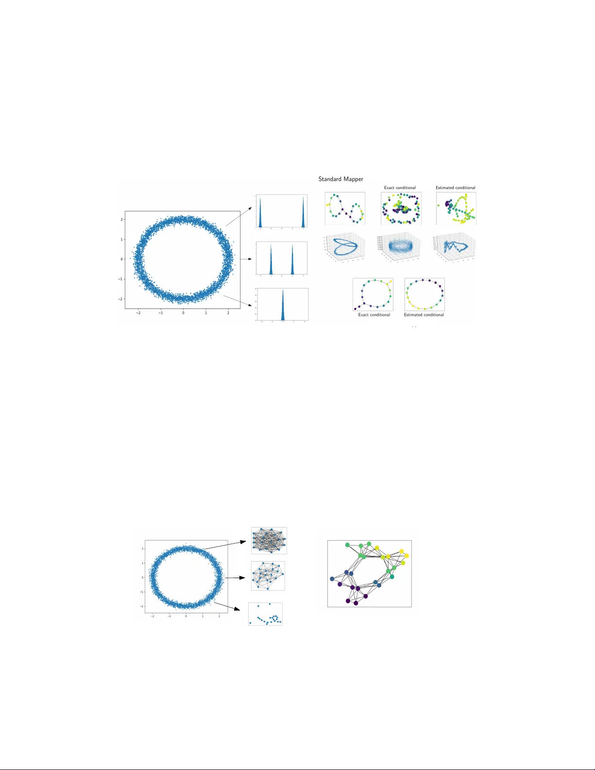
Statistical analysis of Mapp er for sto c hastic and m ultiv ariate ﬁlters Mathieu Carri ` ere ∗ , Bertrand Mic hel † Jan uary 18, 2021 Abstract Reeb spaces, as well as their discretized versio ns called Mapp ers, are common descriptors used in T op ological Data Analysis, with plent y of applications in v arious ﬁelds of science, such as computational biology and data visualization, among others. The stability and quan tiﬁcation of the rate of con vergence of the Mapp er to the Reeb space has b een studied a lot in recent w orks [BBMW19, CO17, CMO18, MW16], focusing on the case where a scalar-v alued ﬁlter is used for the computation of Mapp er. On the other hand, muc h less is known in the multiv ariate case, when the co domain of the ﬁlter is R p , and in the general case, when it is a general metric space ( Z , d Z ), instead of R . The few results that are av ailable in this setting [DMW17, MW16] can only handle con tinuous top ological spaces and cannot be used as is for ﬁnite metric spaces representing data, suc h as p oin t clouds and distance matrices. In this article, we introduce a slight mo diﬁcation of the usual Mapp er construction and we give risk b ounds for estimating the Reeb space using this estimator. Our approach applies in particular to the setting where the ﬁlter function used to compute Mapp er is also estimated from data, suc h as the eigenfunctions of PCA. Our results are given with respect to the Gromov-Hausdorﬀ distance, computed with sp eciﬁc ﬁlter-based pseudometrics for Mapp ers and Reeb spaces deﬁned in [DMW17]. W e ﬁnally pro vide applications of this setting in statistics and mac hine learning for diﬀerent kinds of target ﬁlters, as w ell as numerical experiments that demonstrate the relev ance of our approach. 1 In tro duction The R e eb sp ac e and the Mapp er are common descriptors of T opological Data Analysis (see for instance [CM17]), that can summarize and enco de the top ological features of a giv en data set using a contin uous function, often called ﬁlter , deﬁned on it. As suc h, b oth ob jects ha ve been used tremendously in many diﬀer- en t ﬁelds and applications of data science, including, among others, computational biology [CR18, JCR + 19, NLC11, R CK + 17], computer graphics [GSBW11, SMC07], or mac hine learning [BGC18, NLSKK18]. Mathe- matically sp eaking, the Reeb space is a quotient space and the Mapp er is a simplicial complex. Both ob jects are represen tatives of the topology of the input data set, in the sense that any topological feature that is presen t in these ob jects witnesses the presence of an equiv alent one in the input data. Moreov er, the Mapp er can b e thought of as a more tractable approximation of the Reeb space, whic h, as a quotient space, might b e diﬃcult to describe and compute exactly . In the simpler case where the ﬁlter function is scalar-v alued, the Mapp er and the Reeb space actually b ecome combinatorial graphs, which is wh y they are mostly used for clustering and data visualization. Actually , even when the ﬁlter is m ultiv ariate, i.e., when its domain b elongs to R p with p > 1, it is common to only compute the skeleton in dimension 1 of the Mapp er, so as to make it easy to display and interpret. Even though computation is easier, restricting to scalar-v alued functions can still b e a dramatic simpliﬁcation, since it happ ens quite often in practice that either multiple ﬁlters jointly c haracterize the data—as is the case, for instance, of multiple driv er genes explaining a disease or cell diﬀerentiation—or that the ﬁlter actually takes v alues in spaces more complicated than Euclidean space—as is the case where ﬁlter functions are sto c hastic, making Mapp ers and Reeb spaces computed with mere realizations of the ﬁlter (in Euclidean space) extremely limited. ∗ DataShape, Inria Sophia Antipolis, Biot, F rance, mathieu.carriere@inria.fr † Laboratoire de Math ´ ematiques Jean Leray , UMR C 6629, Ecole Centrale de Nan tes, F rance, bertrand.michel@ec-nantes.fr 1 In recent works, diﬀeren t notions of stabilit y and con vergence of the Mapp er to the Reeb space, in the case where the ﬁlter function is scalar-v alued, hav e b een deﬁned and studied [BGW14, BBMW19, CO17, CMO18, dSMP16], under v arious statistical assumptions on how data is generated. The case of multiv ariate and more general ﬁlter functions is ho w ever m uch more diﬃcult and less understoo d, since the singular v alues of the ﬁlter function, whic h turn out to be critical quantities to lo ok at in the analysis, cannot b e ordered easily , and as a consequence, the natural stratiﬁcation of data (that could b e derived for scalar-v alued Morse functions for instance) do es not extend. F ew av ailable results, presented in [MW16] and [DMW17], prov e nice approximation inequalities for contin uous spaces, but unfortunately do not apply when data is given as a ﬁnite metric space, such as a p oin t cloud or a distance matrix, since those ﬁnite metric spaces should b e though t of as approximations of the underlying contin uous space, and not the space itself. Moreo ver, many of previously cited works only consider the case where the v alues of the ﬁlter function (either scalar-v alued or multiv ariate) are known exactly on the data p oin ts. This will not be the case if the ﬁlter function is estimated from data, and th us diﬀerent from the ﬁlter function used to compute the target Reeb space, as is the case for instance of PCA ﬁlters or density ﬁlters which are abundan t in Mapp er applications. This also happ ens tremendously in statistics and machine learning, where the underlying ﬁlter is usually a predictor, that has to b e estimated with standard machine learning metho ds. As explained in this article, another interesting example is when the interesting and underlying ﬁlter is given by the (scalar- v alued) means, or the (multiv ariate) histograms, of some conditional probability distributions asso ciated to eac h p oin t in the data set, and that what is giv en at hand are merely single realizations of these distributions. Then, the usual wa y of computing Mapp ers will clearly not work, esp ecially if these conditional probability distributions ha ve large v ariances, since single realizations are not represen tative at all of the means, or histograms, of the asso ciated conditional probability distributions. Con tributions. The contribution of this article is tw o-fold: • W e prop ose risk b ounds for the estimation of the Reeb space with a Mapp er-based estimator in the general case, that is, for any type of ﬁlter whose codomain is a complete and lo cally compact length space [BBI01]. F or this, we use the Gromov-Hausdorﬀ distance computed with ﬁlter-based pseudo- metrics deﬁned on Mapp ers and Reeb spaces (and originally introduced in [DMW17]). Our results are stated in the context where the ﬁlter used to compute the Mapper is only an estimation (usually computed from a random sample of data) of the target ﬁlter used to compute the Reeb space. • W e prop ose some metho dology for using our Mapp er-based estimator. W e also provide applications and n umerical experiments in statistics and machine learning, as well as examples in whic h the standard Mapp er fails at recov ering the correct top ology of the data, while using our Mapper-based estimator succeeds at doing so. The plan of this article is as follows: in Section 2, we recall the basics of Reeb spaces, Mapp ers, and we in tro duce the pseudometrics deﬁned on them. Then, we sho w risk b ounds for our Mapp er-based estimator in Section 3. Numerical exp erimen ts and applications are presented in Section 4. Finally , we conclude and pro vide future inv estigations in Section 5. 2 Bac kground on Reeb spaces and Mapp ers In this section, we recall the deﬁnitions of the Reeb spaces and Mapp ers (Section 2.1), and we introduce the Gromo v-Hausdorﬀ distance and the ﬁlter-based pseudometrics that we use to compare them (Section 2.2). 2.1 Reeb spaces and Mapp ers Reeb spaces and Mapp ers are mathematical constructions that enable to simplify and visualize the v arious top ological structures that are present in top ological spaces, through the lens of a contin uous function, often called ﬁlter . 2 Reeb space. Giv en a top ological space X and a con tinuous function f : X → Z , where ( Z , d Z ) is a metric space, the R e eb sp ac e of X is an approximation of X that preserves its connectivit y structures. When f : X → R is scalar-v alued, it is usually called the R e eb gr aph [Ree46]. Deﬁnition 2.1. L et X b e a top olo gic al sp ac e and f : X → Z b e a c ontinuous function deﬁne d on it. The Reeb space of X is the quotient sp ac e R f ( X ) = X / ∼ f , wher e, for al l x, x 0 ∈ X , one has x ∼ f x 0 if and only if f ( x ) = f ( x 0 ) and x, x 0 b elong to the same c onne cte d c omp onent of f − 1 ( f ( x )) = f − 1 ( f ( y )) . Moreo ver, the Reeb space comes with a pro jection π : X → R f ( X ) deﬁned with π ( x ) = [ x ] ∼ f , where [ x ] ∼ f denotes the equiv alence class of x w.r.t. the relation ∼ f . Since f is contin uous, so is π . Appro ximation with Mapp er. Ho wev er, the Reeb space is not well-deﬁned when data is given as a ﬁnite metric space, i.e., a p oin t cloud or a distance matrix, in which case all preimages used to compute the Reeb space are either empty or singletons. T o handle this issue, the Mapp er w as in tro duced in [SMC07] as a tractable approximation of the Reeb space. W e ﬁrst provide its deﬁnition for contin uous spaces. Deﬁnition 2.2. L et X b e a top olo gic al sp ac e and f : X → Z b e a c ontinuous function deﬁne d on it. Mor e over, let U b e a c over of im( f ) , that is, a family of subsets { U α } α ∈ A of Z such that im( f ) ⊆ S α ∈ A U α . L et V b e the c over of X deﬁne d as V = { V ⊆ X : ∃ α ∈ A s.t. V is a c onne cte d c omp onent of f − 1 ( U α ) } . The Mapp er of X , f , U is then deﬁne d as M f , U ( X ) = N ( V ) , wher e N denotes the nerve of a c over. P arameters and extension to p oint cloud. When data is giv en as a ﬁnite metric space, the connected comp onen ts are usually identiﬁed with clustering, and the nerve is computed b y asse ssing a non-empty in tersection b et ween several cov er elemen ts as so on as there exists at least one p oin t that is shared by all these elements. In the remaining of this article, w e use graph clustering. More precisely , we assume that we ha ve a graph G built on top of our ﬁnite metric space, and for each element U of the cov er U , w e use the connected comp onen ts of the subgraph G ( U ) to compute the Mapp er, where G ( U ) is deﬁned as G ( U ) = ( V U , E U ) , (1) where the v ertex set V U is { v ∈ V ( G ) : f ( v ) ∈ U } and the edge set E U is { ( u, v ) ∈ E ( G ) : u ∈ V U , v ∈ V U } ). When G is set to b e the δ -neighborho od graph G δ , this amounts to p erform single-link age clustering [MC12] with parameter δ , and w e let M f , U ,G δ (2) denote the corresp onding Mapp er for ﬁnite metric spaces. Moreo ver, when Z = R p , it is very usual to deﬁne a co ver U with h yp ercubes by cov ering ev ery single dimension of R p with interv als of length r > 0 and ov erlap p ercentage g ∈ [0 , 1], and then by taking the Euclidean pro ducts of these in terv als. Note that r and g are often called the r esolution and the gain of the cov er resp ectiv ely . W e let U ( r , g ) denote this particular t yp e of cov er. Note how ev er that this strategy b ecomes quickly very exp ensiv e, and thus prohibitive, when the dimension p is large. Actually , even for mo derate v alues, e.g., p = 10, the computation can b ecome very costly if the resolution is to o small or the gain is to o large. Moreov er, from a statistical p erspective, suc h a naiv e strategy requires a num b er of observ ations which increases exp onen tially with the dimension, due to the curse of dimensionality . It is thus essen tial to prop ose greedy metho ds to deﬁne eﬃcient cov ers in such situations. In Section 3.1, w e provide alternativ e and computationally feasible strategies to cov er the ﬁlter domain using thic kenings of partitions. It has b een shown in recent works [BBMW19, CO17, CMO18, MW16] that the Mapp er actually approx- imates the Reeb space under v arious assumptions and metrics when the ﬁlter is scalar-v alued. In the next section, we in tro duce the ﬁlter-based pseudometrics that w e will use for comparing Mappers and Reeb spaces with the Gromov-Hausdorﬀ distance. 3 2.2 The ﬁlter-based pseudometric The ﬁlter-based pseudometric, introduced in [BGW14, DMW17], basically measures the diameter of contin- uous paths b et ween any t wo p oin ts r elative to the ﬁlter values . Deﬁnition 2.3. L et X b e a top olo gic al sp ac e and f : X → Z b e a c ontinuous function deﬁne d on it. The ﬁlter-based pseudometric d f : X × X → R is deﬁne d as d f ( x, x 0 ) = inf γ ∈ Γ( x,x 0 ) max t,t 0 ∈ [0 , 1] d Z ( f ◦ γ ( t ) , f ◦ γ ( t 0 )) = inf γ ∈ Γ( x,x 0 ) diam Z ( f ◦ γ ) , wher e Γ( x, x 0 ) denotes the set of al l c ontinuous p aths γ : [0 , 1] → X such that γ (0) = x and γ (1) = x 0 , and diam Z denotes the diameter of a subset of Z . Similarly, the R e eb sp ac e R f ( X ) c an also b e e quipp e d with a pseudometric ˜ d f using the pr oje ction π . F or any two e quivalenc e classes r, r 0 ∈ R f ( X ) , ˜ d f ( r , r 0 ) = d f ( x, x 0 ) for arbitr ary x ∈ π − 1 ( r ) and x 0 ∈ π − 1 ( r 0 ) . Finally , we also deﬁne a pseudometric b et ween the no des of the Mapp er M f , U ( X ). Recall that the no des of the Mapp er are the v ertices of the cov er N ( V ) (see Deﬁnition 2.2), and hence eac h node v corresp onds to a connected comp onen t of f − 1 ( U ) for some U ∈ U . Th us, we can asso ciate an arbitrary (but distinct) elemen t z v ∈ U for each v . Let us introduce the function f U : V (M f , U ( X )) → Z with f U ( v ) = z v . Deﬁnition 2.4. The ﬁlter-b ase d pseudometric is then deﬁne d with ˜ d f , U ( v , v 0 ) = inf γ ∈ Γ( v,v 0 ) max p,q ∈ γ d Z ( f U ( p ) , f U ( q )) , wher e Γ( v , v 0 ) denotes the set of al l p aths b etwe en v and v 0 in M f , U ( X ) , that is, Γ( v , v 0 ) is of the form Γ( v , v 0 ) = { p 1 , . . . , p n : n ∈ N , p 1 = v , p n = v 0 , ( p i , p i +1 ) is an e dge of M f , U ( X ) , ∀ 1 ≤ i ≤ n − 1 } . According to the following prop osition, the spaces X and R f ( X ) (equipped with these pseudometrics) are actually the same when compared with the Gromov-Hausdorﬀ distance [BBI01]. Prop osition 2.5. L et X b e a top olo gic al sp ac e and f : X → Z b e a c ontinuous function deﬁne d on it. Then d GH (( X , d f ) , (R f ( X ) , ˜ d f )) = 0 . Pr o of. Since π is surjectiv e, let C b e the correspondence b etw een X and R f ( X ) deﬁned with π , that is, C = { ( x, π ( x )) : x ∈ X ) } . Let x, x 0 ∈ X . Then the metric distortion of x, x 0 induced b y C is D ( x, x 0 ) := | d f ( x, x 0 ) − ˜ d f ( π ( x ) , π ( x 0 )) | = 0 b y deﬁnition of ˜ d f , and then d GH (( X , d f ) , (R f ( X ) , ˜ d f )) ≤ sup x,x 0 ∈X D ( x, x 0 ) = 0. Let res( U , f ) = max α ∈ A sup u,v ∈ U α ∩ im( f ) d Z ( u, v ) = max α ∈ A diam Z ( U α ∩ im( f )) the resolution of U in Z with respect to the ﬁlter f . It turns out that Mapp ers and Reeb spaces equipped with their resp ectiv e pseudometrics are actually close for cov ers with small diameters. Theorem 2.6 ([DMW17]) . L et X b e a top olo gic al sp ac e and f : X → Z b e a c ontinuous function deﬁne d on it. Then d GH ((M f , U ( X ) , ˜ d f , U ) , (R f ( X ) , ˜ d f )) ≤ 5 · res( U , f ) . 3 Reeb space inference In this section w e prop ose a new Mapp er-based estimator for Reeb spaces in the general framework where the domain ( X , d X ) and the co domain ( Z , d Z ) of the ﬁlter function f are complete and lo cally compact length spaces [BBI01], which in particular means that shortest paths exist for every pair of p oin ts in X and Z (as p er Theorem 2.5.23 in [BBI01]). W e recall that a shortest path b et ween z and z 0 in Z is a con tinuous path γ ∗ : [0 , 1] → Z with γ ∗ (0) = z , γ ∗ (1) = z 0 , suc h that, for any other contin uous path γ : [0 , 1] → Z with γ (0) = z , γ (1) = z 0 , one has | γ ∗ | ≤ | γ | and | γ ∗ | = d Z ( z , z 0 ), where | · | denotes the length asso ciated to Z . 4 The main idea b ehind our estimator is to ﬁrst compute a reﬁnement of the input p oin t cloud in order to remo ve its pathological elements (w.r.t. the cov er used for computing the estimator). These elements are the so-called element-cr ossing e dges , deﬁned in Section 3.2. Then, our estimator is deﬁned as the standard Mapp er estimator for this reﬁned p oint cloud. W e ﬁrst introduce a raw v ersion of the estimator without calibrating the parameters. This calibration is then detailed further and allows to provide a risk b ound for our corresp onding estimator. 3.1 A Mapp er-based estimator In this section, w e in tro duce our Mapp er based estimator in a deterministic setting. Assume that tw o p oin t clouds X n and Z n are given: X n = ( x 1 , . . . , x n ) and Z n = ( z 1 , . . . , z n ) such that for any i , one has ( x i , z i ) ∈ X × Z and z i = ˆ f ( z i ). The function ˆ f : X n → Z is an appro ximation of a “true” and unkno wn ﬁlter function f : X → Z . In some settings, the true exact ﬁlter f is known and then we simply hav e ˆ f = f | X n . P oint cloud and em b edded graph. W e let G δ b e the (metric) neigh b orho od graph built on top of X n with parameter δ , that is, any pair { x i , x j } ⊆ X n creates an edge in G δ , with length d X ( x i , x j ), and parameterized with a shortest path b et w een x i and x j , if and only if d X ( x i , x j ) ≤ δ . W e then deﬁne the corresp onding emb e dde d gr aphs as G Z δ (resp. ˆ G Z δ ) in Z , with vertices { f ( x i ) : x i ∈ X n } (resp. { ˆ f ( x i ) : x i ∈ X n } ) and whose edges are geometric realizations of edges of G δ , that is, shortest paths in Z 1 . When Z is a normed v ector space (such as a Banach space), this corresp onds to linear interpolations in Z . W e ﬁnally extend f | X n (resp. ˆ f ) to a function f PG : G δ → G Z δ (resp. ˆ f PG : G δ → ˆ G Z δ ), which maps the interiors of the edges of G δ to the corresp onding interiors of the shortest paths in Z . Note that f | X n and f PG (resp. ˆ f and ˆ f PG ) coincide on X n , so we will only use f PG (resp. ˆ f PG ) when applied to (interiors of ) edges of G δ . Graph reﬁnemen t. Our Mapp er-based estimator is deﬁned as the standard Mapp er computed on a reﬁnemen t of the graph G δ . F or s ∈ N ∗ , we sub divide each edge of G δ with s p oin ts. Let G δ,s b e the resulting graph (on which f PG and ˆ f PG are still well-deﬁned), X n,s b e the reﬁned p oin t cloud, and G Z δ,s , ˆ G Z δ,s b e the reﬁned embedded graphs. Co ver. Let U be a ﬁnite co ver of im( ˆ f PG ), whic h can b e data dep endent. F or no w, we assume that this co ver is given. W e will discuss the construction of U further in this article. Estimator. W e are now in p osition to deﬁne our Mapp er based estimator. It is deﬁned with (2) as: M n = M ˆ f PG , U ,G δ,s ( X n,s ) , (3) and it can b e equipp ed with the pseudometric ˜ d ˆ f PG , U of Deﬁnition 2.4. See Figure 1 for an illustration of the construction of M n . F or deﬁning the estimator, we need to choose the scale parameters s and δ , and w e discuss this question further in the next section. 3.2 Risk b ound and parameter calibration W e now give our main result in the Sto chastic Filter setting , i.e., when the data X 1 , . . . , X n are sampled i.i.d. from a distribution P and when the function ˆ f : X n → Z is allow ed to b e data dep enden t. In this setting the Z i ’s are thus also i.i.d. random v ariables. • (H1) Supp ort Assumption. The supp ort X of P is a compact submanifold X ⊆ R D with p ositiv e reac h rc h( X ) (see [BL W19] for deﬁnitions). The neighborho od graph G δ is built with Euclidean norm k · k in R D . Let D X < ∞ denote the diameter of X (in the Euclidean distance). Hereafter, we call rch( X ) and D X the ge ometric p ar ameters of X . 1 Our construction actually works for arbitrary paths. How ever, some quantities that are necessary for computing the estimator (suc h as ` ) might b e easier to compute when working with shortest paths, so we stick to those paths in this article. 5 Z a b c d e a b c d e a b c c d d e a b c d e c d a b c d e c d 1 2 3 3 3 1 3 4 5 5 ˆ f PG X M n M ˆ f PG , U M ˆ f , U ,δ n a b c d e 3 4 5 1 2 Figure 1: Example of our estimator M n on a dataset of 5 p oints. Upp er left: Dataset X n with ﬁve p oin ts a, b, c, d, e . The edges b et ween the p oints are computed with a neigh b orho od graph with parameter δ n . Upp er righ t: Cov er of im( ˆ f PG ) with four squares. The edges b et ween the p oin ts in Z are shortest paths in Z . Low er left: Preimages of the four squares for the standard Mapp er on the p oin t cloud and corresp onding simplicial complex computed with hierarchical clustering with parameter δ n . Lo wer right: Preimages of the four squares for the standard Mapp er on the metric neighborho o d graph. Lo wer middle: Our estimator is computed by reﬁning the neigh b orhoo d graph (with ﬁve extra nodes 1 , 2 , 3 , 4 , 5) and b y using this new graph to compute the connected comp onen ts and the intersections b et ween them. • (H2) Measure Assumption. The probabilit y measure P is ( a, b )-standard, i.e., P ( B ( x, r )) ≥ min { 1 , ar b } , for all x ∈ X and r > 0, where B ( x, r ) = { y ∈ R D : k y − x k ≤ r } . By assumption, the ﬁlter of a Reeb graph is a con tinuous function. The ﬁlter function f is thus uniformly con tinuous on the compact set X and it admits a minimal mo dulus of contin uit y ω f . The function ω f is a non-decreasing function such that for any u ∈ R + , ω f ( u ) = sup  d Z ( f ( x ) , f ( x 0 )) : ( x, x 0 ) ∈ X 2 and k x − x 0 k ≤ u  . The domain X b eing compact, ω f satisﬁes (see for instance Section 6 in [DL93]) 1. ω f ( δ ) → ω (0) = 0 as δ → 0; 2. ω f is non negative and non-decreasing on R + ; 3. ω f is subadditive : ω f ( δ 1 + δ 2 ) ≤ ω f ( δ 1 ) + ω f ( δ 2 ) for any δ 1 , δ 2 > 0; 4. ω f is contin uous on R + . 6 In this article, w e say that a function ω deﬁned on R + is a mo dulus of c ontinuity if it satisﬁes the four prop erties ab o ve and w e sa y that it is a mo dulus of c ontinuity for f if, in addition, we hav e | f ( x ) − f ( x 0 ) | ≤ ω ( k x − x 0 k ) , for any x, x 0 ∈ X . • (H3) Filter Regularity Assumption. The true ﬁlter f : X → Z is a contin uous function on X whic h admits a mo dulus of contin uity ω suc h that x ∈ R + 7→ ω ( x ) x is a non-increasing function on R + . Finally , we will assume the following assumption on the cov er: • (H4) Cov er Assumption. The cov er U is assumed to co ver im( ˆ f PG ). F or calibrating the estimator parameters, w e need to introduce the notion of element-cr ossing e dges . Such edges are pathological in the sense that they may preven t to recov er the correct top ology of the underlying Reeb space. Giv en a simplex σ = { U α 1 , . . . , U α p } in the nerve N ( U ), we let U σ = ∩ p i =1 U α i . Deﬁnition 3.1. L et ( X i , X j ) ∈ X 2 n such that the e dge e = ( X i , X j ) b elongs to G δ . L et ˆ f PG ( e ) b e the c orr esp onding e dge in ˆ G Z δ . We say that e is an elemen t-crossing edge with resp ect to the cov er U if ther e exists σ ∈ N ( U ) such that ˆ f PG ( e ) ∩ U σ 6 = ∅ , ˆ f ( X i ) 6∈ U σ and ˆ f ( X j ) 6∈ U σ . In other words, e is an element-crossing edge with resp ect to the cov er U if the shortest path ˆ f PG ( e ) go es through U σ , ev en though its endp oints ˆ f ( X i ) and ˆ f ( X j ) are outside U σ . In this case we say that U σ is cr osse d by e . Note that element-crossing edges are generalizations of interval and interse ction-cr ossing e dges , as deﬁned in [CO17]. W e then deﬁne: ` ( X n , ˆ f , U ) = inf n | ˜ e | , where ˜ e is a c.c. of ˆ f PG ( e ) ∩ U σ , e is element-crossing and U σ is crossed by e o , where | ·| denotes the length in Z and c.c. is a shorthand for connected component. In other words, ` ( X n , ˆ f , U ) is the length of the smallest connected path in the intersection b et w een an edge of ˆ G Z δ and a cov er element or intersection, such that the edge endp oin ts do not b elong to this cov er element or intersection. F or calibrating the parameters, we also need to introduce the mo dulus of con tinuit y of ˆ f PG : ˆ ω PG ( h ) = sup n d Z ( ˆ f PG ( x ) , ˆ f PG ( x 0 )) : k x − x 0 k ≤ h and x, x 0 b elong to the same edge of G δ o , where | · | denotes the edge length in G δ . W e are now in p osition to deﬁne the calibrations for δ and s . W e follow a similar strategy as in [CMO18]. Let d E H denotes the Hausdorﬀ distance [BBI01] computed with Euclidean distances. • Choice for δ . F or some arbitrary β > 0, let s ( n ) = n/ (log( n )) 1+ β . W e take δ = δ n = d E H ( ˜ X s ( n ) , X n ) , (4) where ˜ X s ( n ) is a random subsample of size s ( n ) dra wn uniformly from X n with replacement. • Choice for s . Let ` = ` ( X n , ˆ f , U ), w e tak e s ≥ s n :=  δ n ˆ ω − 1 PG ( `/ 2)  if `/ 2 ∈ im( ˆ ω PG ) (5) and s n = 0 (that is, we do not reﬁne G δ ) otherwise. By conv ention, w e also let s n = + ∞ if ` = 0, whic h happ ens with null probability . Under the previous assumptions and with the deﬁnitions of s n and δ n giv en abov e, w e can pro vide the follo wing risk b ound of our Mapp er based estimator: 7 Theorem 3.2. Under assumptions (H1) , (H2) , (H3) and (H4) , the fol lowing ine quality is true: E h d GH ((M n , ˜ d ˆ f PG , U ) , (R f ( X ) , ˜ d f )) i ≤ 5 E h res( U , ˆ f PG ) i + C ω  C 0 log( n ) (2+ β ) /b n 1 /b  + 2 E h k f PG − ˆ f PG k ∞ i , wher e the c onstants C , C 0 only dep ends on a , b and the ge ometric p ar ameters of X , and wher e the thir d term is deﬁne d with k f PG − ˆ f PG k ∞ := sup x ∈ G δ n d Z ( f PG ( x ) , ˆ f PG ( x )) . The pro of is given App endix A.1. Note that this result is v ery general and can handle random or data dep enden t co vers for instance. W e discuss co ver c hoices and corresp onding upper bounds on their resolutions in Section 3.3. Moreov er, e v en though the third term might b e diﬃcult to control for general length spaces, when Z is a Hilb ert space it actually reduces to E h k f PG − ˆ f PG k ∞ i = E h k ( f − ˆ f ) | X n k ∞ i , since shortest paths are straight lines in such spaces. This is the case for instance when Z is a repro ducing k ernel Hilb ert space (RKHS), whic h w e study in more details further in Section 3.4. P arameter calibrations. Theorem 3.2 relies on the calibration of the parameters of our Mapp er-based estimator M n . In particular, the choice w e make for the graph reﬁnement parameter s requires to: ﬁrst, upp er b ound the mo dulus of con tinuit y ˆ ω PG of ˆ f PG , and second, to compute the smallest connected path ` ( X n , ˆ f , U ). Controlling ˆ ω PG is not p ossible in general, but for standard ﬁlters such as KPCA ﬁlters (see Section 3.4), ˆ f and ˆ f PG are Lipschitz functions and hence ˆ ω PG can b e easily b ounded by the corresp onding Lipsc hitz constan t. Next, computing—or at least low er b ounding—the quantit y ` ( X n , ˆ f , U ) is diﬃcult for a general cov er U . How ev er, it can b e done exactly for particular cov ers, such the ones induced by thick ening K -means or V oronoi partitions in Hilb ert spaces (see Section 3.3). Indeed, in this case, it is p ossible to test whether a given shortest path intersects a cov er element or intersection by computing the intersection of the line induced by the shortest path—which is p ossible since shortest paths are segments—and all the mediator lines that form the b oundary of the cov er element. In practice, when ˆ ω PG and ` ( X n , ˆ f , U ) are diﬃcult to compute, we adopt a conserv ativ e approach by considering for the graph reﬁnement parameter s the largest p ossible integer that still allows our estimator to b e computed with a reasonable amount of time and memory usage, dep ending on the machine that is b eing used. Finally , it should b e noted that small sizes of cov er elements or intersections induce small ` and large s , and thus p oten tially longer computation times. 3.3 Co v er control In this section, we study the resolutions of cov ers induced b y V oronoi partitions. In particular, we deﬁne those cov ers in Section 3.3.1, and provide upp er b ounds on their resolutions in Section 3.3.2. This allows to form ulate more explicit upp er b ounds for the ﬁrst term in Theorem 3.2. 3.3.1 Deﬁning co v ers Co vers with h yp ercubes is the most common co ver used with Mappers when Z = R p when p is not too large. When the ﬁlter domain Z is a general length space, as for instance when Z is the space of probability distributions of R (see Section 4.2) or when Z is a space of combinatorial graphs (see Section 4.3), we need an alternative construction to deﬁne cov ers. A simple wa y of generating a co ver is b y using a partition of this space, and thick ening the elemen ts of this partition. Deﬁnition 3.3. L et ( Z , d Z ) b e a length sp ac e, and let  > 0 . • F or U ⊆ Z a subset of Z , the  -thic kening of U is deﬁne d as U  = { z ∈ Z : inf { d Z ( z , ˜ z ) : ˜ z ∈ U } ≤  } . • L et e Z b e a subset of Z and let U = { U α } α ∈ A b e a p artition of e Z , i.e., e Z ⊆ S α ∈ A U α and U α ∩ U β = ∅ for al l α 6 = β ∈ A . The  -thic kening of U for c overing e Z is deﬁne d as U  = { U  α } α ∈ A . 8 Ev en when Z = R p , it might b e interesting to use thick enings of partitions instead of h yp ercub e cov ers, since the num b er of hypercub es increases exp onen tially with the dimension p , with many of them ha ving an empt y preimage under f , and thus useless. Note also that when our Mapp er-based estimator is used with an  -thick ening cov er, our estimator gets more diﬃcult to compute when the thick ening parameter  go es to zero, since it requires reﬁning the initial neigh b orho od graph with a lot of new vertices. 3.3.2 Bounding the resolution for  -thick ening of V oronoi partitions Under the same general assumptions as Section 3.2, w e consider the sp eciﬁc case where Z = R p endo wed with the inner pro duct h· , ·i . Partitions of R p can b e computed very eﬃcien tly , for instance with V oronoi partitions and the k -means algorithm. In this section we giv e an upper b ound on the resolution term in volv ed in the upp er b ound of Theorem 3.2, for a cov er computed from a k -means algorithm. Deﬁnition 3.4. F or Q a me asur e in R p and k ∈ N ∗ , a set t ( Q ) of k p oints in R p is said to b e k -optimal for Q if t ( Q ) ∈ argmin t ∈ ( R p ) k Z Z min i =1 ,...,k k z − t i k 2 2 dQ ( z ) . Let P ˆ f n b e the push forward measure of P n b y the sto c hastic ﬁlter function ˆ f , where P n is the empirical measure asso ciated to X n . Of course, all these quantities are deﬁned conditionally to the sample X n and ˆ f (in particular if ˆ f dep ends on other observ ations Y n , as w ould b e the case, e.g., in the context of a regression function ﬁlter). Note that P ˆ f n is equiv alently deﬁned as the empirical measure corresp onding to the observ ation of the sample Z n = ˆ f ( X n ). The k -means algorithm on Z n aims at approximating an optimal k p oin ts for the empirical measure P ˆ f n from the observ ation Z n . Let ˆ t = t ( P ˆ f n ) b e an optimal k -points for the empirical measure P ˆ f n . W e denote by b U  = { ˆ U  j } j =1 ,...,k the  -thick ening of the V oronoi partition associated to ˆ t . Since Z = R p , we know that ˆ f PG is a linear in terp olation b et ween the Z i ’s. Th us b U  is a cov er for im( ˆ f PG ) and Assumption (H4) is satisﬁed. W e give our result under the additional assumption that the minimal mo dulus of contin uit y ω is upper b ounded b y a concav e function of the form ¯ ω ( u ) = cu γ , with c ≥ 0 and 0 < γ ≤ 1. This assumption is ob viously stronger than Assumption (H3). • (H5) P o wer function upp er b ounds ω . There exists γ ∈ (0 , 1] and c ∈ R + suc h that for any u ∈ R + , ω ( u ) ≤ ¯ ω ( u ) = cu γ . This technical assumption allows us to provide a simple upp er b ound. Note that it makes sense b ecause on the compact set X , the minimal mo dulus of contin uity ω is indeed a concav e function. The next result gives a control on the resolution of b U  in R p with resp ect to the ﬁlter function ˆ f PG . Theorem 3.5. Under assumptions (H1) , (H2) and (H5) , for Z = R p and for k ≤ n p +2 , the r esolution of the c over b U  in R p with r esp e ct to the ﬁlter function ˆ f PG satisﬁes E h res( b U  , ˆ f PG ) i ≤ C 1 " k − 2 γ 2 b 2 +2 γ b +  k p n  γ 2 b +4 γ + E k ( f − ˆ f ) | X n k ∞ # + 2 ε. (6) Conse quently, the fol lowing risk b ound holds for our Mapp er b ase d estimator M n = M ˆ f PG , b U  ,G δ,s ( X n,s ) : E h d GH ((M n , ˜ d ˆ f PG , b U  ) , (R f ( X ) , ˜ d f )) i ≤ C 2 " k − 2 γ 2 b 2 +2 γ b +  k p n  γ 2 b +4 γ + E k ( f − ˆ f ) | X n k ∞ # + 10 ε. (7) Mor e over, the c onstants C 1 and C 2 dep ends on a , b , c , γ , k f k ∞ and on the ge ometric p ar ameters of X . The pro of of Theorem 3.5 is giv en in Section A.2, in which several ideas from [BL20] are reused and adapted. Note that we could also provide a deviation b ound on the resolution by applying the so-called Bounded Inequality in a standard wa y (see for instance Theorem 6.2 in [BBL05]). 9 Rate of conv ergence. Assuming that γ and b are known, we can c ho ose k to balance the ﬁrst tw o terms in the brack et of the righ t hand side of Inequality (7). By taking k of the order of  n p  b 2 +2 γ b ( b +2 γ )(4 γ + b ) , we obtain that the ﬁrst tw o terms in the brack et are of the order of ε n :=  p n  ζ with ζ := 2 γ 2 ( b +2 γ )(4 γ + b ) < 1 4 . If the con vergence of ˆ f to f is faster than ε n , and taking a resolution ε of the order of ε n , we ﬁnally obtain that the expected risk of our Mapp er based estimator is of the order of ε n . W e conjecture that this rate of con vergence is not optimal, how ever it can b e used to sho w the consistency of our Mapp er-based estimator. 3.4 Application to KPCA ﬁlters In this section, we study the upp er b ounds of Theorem 3.2 in the particular case where Z is a repro ducing k ernel Hilb ert space (RKHS). Let Z b e a RKHS asso ciated to a contin uous kernel function K deﬁned on X × X . The set X being compact and K being contin uous, Z is then a separable RKHS. Moreov er, the feature map x 7→ K ( x, · ) is a contin uous function from X to Z since: k K ( x, · ) − K ( x 0 , · ) k 2 Z = K ( x, x ) + K ( x 0 , x 0 ) − K ( x, x 0 ) − K ( x 0 , x ) . (8) Moreo ver, the random v ariable Z = K ( X , · ) is b ounded in Z since k K ( X, · ) k 2 Z = K ( X, X ) which is almost surely b ounded on the compact space X . In particular, E  k K ( X, · ) k 2 Z  < ∞ . In this setting, the cov ariance op erator of the distribution of Z is w ell deﬁned (see for instance Section 2 and 4.1 in [BBZ07]). T o simplify , w e will assume that the distribution of Z is centered. Co v ariance op erator. Let Γ = E ( Z ⊗ Z ∗ ) b e the cov ariance op erator and let Π p b e the orthogonal pro jection op erator on the set of the ﬁrst p eigenv ectors of Γ. The op erator Γ can b e approximated by its empirical version: Γ n = 1 n n X i =1 Z i ⊗ Z ∗ i where Z i = K ( X i , · ). Let ˆ Π n,p b e the orthogonal pro jection op erator on the set of the ﬁrst p eigenv ectors of Γ n . In this section, w e consider as ﬁlter functions the comp osition of the feature map with one of the t wo pro jection op erators: f p : x ∈ X 7→ Π p ( K ( x, · )) and ˆ f n,p : x ∈ X 7→ ˆ Π n,p ( K ( x, · )) . Mo dulus of contin uit y . Let ω K b e the mo dulus of contin uity of K : for any ( x 1 , x 2 , x 0 1 , x 0 2 ) ∈ X 4 , | K ( x 1 , x 2 ) − K ( x 0 1 , x 0 2 ) | ≤ ω K  q k x 1 − x 0 1 k 2 + k x 2 − x 0 2 k 2  , where k · k is the euclidean norm of R D . Let ( x, x 0 ) ∈ X 2 , then k f p ( x ) − f p ( x 0 ) k Z = k Π p ( K ( x, · )) − Π p ( K ( x 0 , · )) k Z ≤ k K ( x, · ) − K ( x 0 , · ) k Z ≤ p 2 ω K ( k x − x 0 k ) where the last inequality comes from (8). This shows that √ 2 ω K is a mo dulus of contin uity for f p . Upp er b ound. The statistical analysis of PCA in Hilbert spaces has b een the sub ject of sev eral works, see for instance [R W + 20, BBZ07, BM12, STW CK05]. Here, we need a control for the sup norm b etw een the ﬁlter and its empirical version. According to Theorem 2.1 in [BM12]: E " sup z ∈Z , k z k Z ≤ 1 k Π p ( z ) − ˆ Π n,p ( z ) k Z # ≤ C √ n 10 where the constant C only dep ends on p . Since X is compact and x 7→ K ( x, · ) is contin uous, it follows that: E  sup x ∈X k f p ( x ) − ˆ f n,p ( x ) k Z  ≤ C 0 √ n where C 0 dep ends on D X and p . Under assumptions (H1), (H2) and (H5), if w e perform a k -means algorithm in the space of the p ﬁrst components of the KPCA to derive a co ver as explained in Section 3.3.2, we can then apply Theorem 3.5 to our corresp onding Mapp er-based estimator. The conv ergence of the estimated ﬁlter in O (1 / √ n ) is fast enough so that it do es not slow down the con vergence of our Mapper-based estimator. F or k and ε chosen as in the discussion following Theorem 3.5, we ﬁnally obtain that the risk of our Mapp er based estimator can b e upp er b ounded by a term of the order of  p n  2 γ 2 ( b +2 γ )(4 γ + b ) . 4 Applications of Mapp er in the Sto c hastic Filter setting In this section, w e fo cus on examples and applications of the Sto chastic Filter setting (see Section 3), in whic h the ﬁlter ˆ f used to compute the Mapp er is assumed to b e an estimation (computed from the data sample) of the true target ﬁlter f used to compute the Reeb space. W e ﬁrst provide in Section 4.1 v arious examples of sto c hastic ﬁlters in statistics and machine learning. Indeed, standard metho ds provide estimated regression functions and classiﬁcation probabilit y estimates which are in teresting to study with Mapp er. Then, we turn the fo cus to the length space of probability distributions in Section 4.2, and we ﬁnally pro vide an illustration for the length space of com binatorial graphs with the graph edit distance in Section 4.3. Throughout this section, the Mapp ers that are computed and discussed alwa ys refer to our Mapp er-based estimator. 4.1 Sto c hastic Filter in Statistical Mac hine Learning In this section, we discuss the v arious p oten tial applications of Mapp ers in statistical machine learning, in whic h the ﬁlter is often used for inference and prediction, and w e provide asso ciated numerical exp erimen ts and illustrations. W e also refer the interested reader to [HTF03] for more details on the statistical and mac hine learning metho ds used in this section. Sto c hastic real-v alued ﬁlters. W e ﬁrst consider a few applications in which the estimated and true target ﬁlters are real-v alued functions, i.e., Z = R . In this setting, one can apply either the risk b ound given in Theorem 3.2 or the results from [CMO18] to quantify the approximation and conv ergence of Mapp er. • Inference. When the target ﬁlter function only dep ends on the measure P itself, w e can deﬁne estimators of this ﬁlter using the p oint cloud X n alone. F or instance, a dimension reduction ﬁlter (e.g. PCA), the eccentricit y ﬁlter or the densit y estimator ﬁlter are all estimators of underlying ﬁlters deﬁned from P . See for instance [CMO18] for examples. • Regression. W e no w assume that we observe a random v ariable Y i at each p oin t X i : Y i = f ( X i ) + ε i , i = 1 , . . . , n (9) where the true ﬁlter is f ( x ) = E ( Y | X = x ), i.e., the regression function on X and ε i = Y i − f ( X i ). Then, the Mapp er of X n can b e computed with any estimator ˆ f of f (from the statistical regression literature) in order to infer the Reeb space R f ( X ). • Binary classiﬁcation. W e now assume that we observe a binary v ariable Y i ∈ {− 1 , 1 } at eac h p oint X i of the sample. Let f ( x ) = P ( Y = 1 | X = x ) b e the probability of class 1 for an y x ∈ X . In this setting, inferring the target Reeb space R f ( X ) with a Mapp er computed on X n for some estimator ˆ f of the class probability distribution (given by an y mac hine learning classiﬁer) w ould provide insights ab out how data is top ologically stratiﬁed w.r.t. the conﬁdence given by the classiﬁer. Extension to sto c hastic multiv ariate ﬁlters. F or many problems in statistical machine learning, the quantit y of interest is actually a m ultiv ariate quantit y . In this setting, using Theorem 3.2 allows to statistically control the quality of Mapp er, whic h, to our knowledge, is new in the Mapp er literature. 11 • Dimension reduction. In this setting, a natural extension of real-v alued inference described ab ov e is the pro jection onto the p ﬁrst directions of an y dimension reduction algorithm. The corresp onding Mapp er is now a m ultiv ariate Mapp er and the underlying ﬁlter is the pro jection on to the p ﬁrst directions of the cov ariance op erator of P . See Section 3.4 ab ov e. • Multiv ariate regression. Multiv ariate regression is the generalization of (univ ariate) regression when the v ariable Y in Equation (9) is now a random vector. • Multi-class classiﬁcation. W e observe a categorical v ariable Y i ∈ { 0 , . . . , k } at each p oin t X i . Let f k ( x ) = P ( Y = k | X = x ) b e the probability of class k at x ∈ X . The underlying ﬁlter is now the v ector of estimated probabilities f = ( f 0 , . . . , f k ), whic h can b e obtained with classiﬁcation metho ds in statistical machine learning. Syn thetic example. W e no w describ e tw o multi-class classiﬁcation problems and display the corre- sp onding Mapp ers. In the ﬁrst one, we generated a data set in t wo dimensions with three diﬀerent classes whic h are en tangled with eac h other. See Figure 2 (left) for an illustration. W e then trained a Random F orest classiﬁer on this data set, and computed the estimated probabilities for each of the training p oin ts, meaning that we hav e an estimated m ultiv ariate ﬁlter ˆ f : R 2 → [0 , 1] 3 . The corresp onding Mapp er (computed with 10 interv als and ov erlap 30% for eac h class) is shown in Figure 2 (righ t). Moreo ver, the Mapp er no des are colored with the v ariance of the class probability distributions: the smaller the v ariance, the more conﬁdent the prediction. It is clear from the Mapp er that the classiﬁer induces a top ological stratiﬁcation of the data, in the sense that p oints in the middle of the space (lo cated in the middle of the triangle-shap ed Mapp er), on whic h the classiﬁer is unsure, connect with p oin ts for which the classiﬁer hesitates b et ween tw o classes (lo- cated in the middle of the “edges” of the triangle), which themselv es connect with p oin ts where the classiﬁer is conﬁdent (lo cated at the “corners” of the triangle), leading to some non-trivial 1-dimensional top ological features in the data, which are not visible at ﬁrst sight on the data set. W e b elieve this visualization could b e of great help when it comes to interpreting the output of standard statistical machine learning metho ds. Figure 2: Three lab el classiﬁcation problem and its corresp onding Mapp er. Left: we generate p oin ts in 2D with three diﬀerent groups (red, purple, green). Right: Mapp er computed with the p osterior probability of a Random F orest classiﬁer. No des are colored with the v ariance of the estimated probabilities from lo w (y ellow) to large (dark blue). Accelerometer data. In our second example, w e study a data set of time series obtained from ac- celerometers placed on p eople doing six p ossible ty p es of activities, namely “standing”, “sitting”, “la ying”, “w alking”, “walking upstairs” and “walking do wnstairs”. F rom the raw data, 561 features hav e b een ex- tracted from sliding window, see [AGO + 13] and the data website 2 for more details. A Naive Bay es classiﬁer has b een trained on the 7 , 352 observ ations. W e ﬁnally generated an asso ciated Mapp er with the corre- sp onding estimated probabilities (computed with 3 in terv als and 30% gain for each class), and we colored the no des with v ariance, similarly to what was done ab o ve. W e show the Mapp er, as well as representativ e time series for some of its no des, in Figure 3. Again, the classiﬁer is inducing a top ological stratiﬁcation 2 https://archive.ics.uci.edu/ml/datasets/Human+Activity+Recognition+Using+Smartphones 12 of the data, with tw o connected comp onen ts (corresp onding to the tw o global types of activities, namely w alking activities or stationary activities), which are themselves stratiﬁed into three activities connected by time series where the classiﬁer is unsure. Sitting Standing W alking up W alking W alking down Intermediate between laying and sitting Laying Figure 3: Mapp er computed on accelerometer data with the p osterior probability of a Naive Ba yes classiﬁer. No des are colored with the v ariance of the estimated probabilities from low (yello w) to large (dark green). 4.2 Sto c hastic Filter with Conditional Probabilit y Distributions W e now assume that w e observe an i.i.d sample { ( X i , Y i ) : 1 ≤ i ≤ n } , where X i ∈ X and Y i ∈ R . In this setting, we prop ose to consider the more complex ﬁlter function whic h is deﬁned as the conditional distribution ( Y | X ): the v alue of this ﬁlter at x is the conditional distribution ( Y | X ). In this framework, the ﬁlter domain is thus the space of probabilit y distributions. In practice, it might b e tempting to directly compute the standard Mapp er with the Y i ’s as ﬁlter v alues. Ho wev er, this approach do es not really make sense b ecause there is no reason for this Mapp er to conv erge to a deterministic Reeb space for some underlying ﬁlter function. Ha ving in mind that the relev an t target ﬁlter is the conditional probability distribution ( Y | X ), it is clear that this naive approach is not a go od strategy for this aim, since single observ ations can b e very p o or estimates of the corresp onding distributions. 4.2.1 Mapp er with probability distributions Let P b e the set of probability measures on R . F or x ∈ X , let ν x b e the conditional distribution ( Y | X = x ). Let ν b e the ﬁlter ν : x ∈ X 7→ ν x ∈ P . V arious metrics can b e prop osed on P , one of them b eing the Prokhoro v metric [Bil13], which metrizes weak conv ergence. Generally sp eaking, the Reeb space R ν ( X ) is diﬃcult to infer since it requires to estimate the conditional probability distribution ν x for all p oin ts of X , whic h is a diﬃcult task, esp ecially for high dimensional data—see for instance [Efr07]. As far as we know, conditional densit y estimation on submanifolds has not b een studied yet. Moreov er, as so on as ν is injec- tiv e, which is not a strong assumption in practice, the Reeb space will b e isomorphic to X and it will not pro vide more information than standard manifold learning pro cedures [MF11]. W e thus propose to study appro ximations of R ν ( X ), using a ﬁlter that is a simple descriptor (suc h as the mean or the histogram) of ν x . In this situation, from a data analysis p erspective, crude approximations of the Reeb space shows more in teresting patterns than those provided b y the Reeb space itself. Mean- and histogram-based Mapp ers. Let I = ( I 1 , . . . , I d ) b e a partition of R with interv als. W e deﬁne the histogram ﬁlter Hist asso ciated to I by Hist j ( x ) = P ( Y ∈ I j | X = x ) for j = 1 , . . . , d . The 13 co domain of Hist is in R d , i.e., it is a multiv ariate ﬁlter, with corresp onding Reeb space R Hist ( X ). W e then prop ose to compute the Mapp er with an estimated histogram, which we call the histo gr am-b ase d Mapp er , using the Nadaray a-W atson kernel estimator: d Hist j ( x ) = P i =1 ,...,n 1 Y i ∈ I j K h ( X i − x ) P i =1 ,...,n K h ( X i − x ) where K h ( x ) = 1 h K ( x h ) for a kernel function K , which we choose, in practice, to b e the indicator function of the unit ball in the ambien t Euclidean space. Note that a simpler approach is to estimate the (conditional) mean f ( x ) = E ( Y | X = x ), and we call the corresp onding estimator the me an-b ase d Mapp er . How ever, as illustrated in n umerical exp erimen ts presen ted b elo w, it may b e not suﬃcient to retrieve interesting data structure. 4.2.2 Numerical experiments W e now provide examples of computations of our Mapp er-based estimators computed from single realiza- tions of syn thetic conditional probability distributions 3 . W e generate 5 , 000 p oin ts from an ann ulus, and w e lo oked at tw o conditional distributions for each p oin t, namely Gaussians and bimo dal ones. See Figure 4 and 5. In eac h of these ﬁgures, we displa y ﬁv e Mappers: the standard Mapper, the mean-based Mapper when the true conditional mean is supp osed to b e known, the mean-based Mapp er when this mean is estimated, the histogram-based Mapp er when the true histogram is supp osed to be known, and the histogram-based Mapp er when the histogram is estimated. W e also plot, for the standard Mapp er and the mean-based Mapp ers, a 3D embedding of the data set, with the mean v alues used as height. F or the standard Map- p er and the mean-based Mapp ers, we used an in terv al co ver with 15 in terv als and ov erlap p ercen tage 30%. F or the histogram-based Mapp er, we used histograms with 100 bins and an 0 . 5-thick ening of a K -PDTM co ver [BL20] with K = 10 cov er elements. Gaussian conditional. In Figure 4, w e generated Gaussian conditional probability distributions cen- tered on the second co ordinates of the points. It can b e seen that the standard Mapper reco vers the underlying structure, but in a v ery imprecise wa y , in the sense that the feature size is m uch smaller than it should b e, due to the v ariances of the distributions that induce very noisy ﬁlter v alues. On the other hand, the mean-based Mapp ers and the histogram-based Mapp ers all recov er the correct structure in muc h more precise fashion. Mean-based Mapp er Histogram-based Mapp er Figure 4: Standard, mean- and histogram-based Mapp ers computed with exact and estimated Gaussian conditional probability distributions. 3 Our code is freely av ailable at https://github.com/MathieuCarriere/metricmapper 14 Bimo dal conditional. In Figure 5, we generate bimo dal conditional probability distributions whose mo des are cen tered on the second co ordinate and its opposite (min us the minimum of the coordinates v alues). This w ay , all conditional probabilit y distributions hav e the same mean. This time, the standard Mapp er gets fo oled b y the probability distributions, and outputs tw o top ological structures instead of one, due to the tw o mo des of the distributions. The mean-based Mapp ers also fail due to the fact that the distributions all hav e the same mean, whic h mixes all p oints together and makes topological inference very diﬃcult, leading to v ery noisy Mapp ers. On the other hand, the histogram-based Mapp ers b oth manage to retrieve the correct structure in a precise wa y . Mean-based Mapp er Histogram-based Mapp er Figure 5: Standard, mean- and histogram-based Mapp ers computed with exact and estimated bimo dal conditional probability distributions. 4.3 Sto c hastic ﬁlter with com binatorial graphs W e end this application section b y pro viding an example of our Mapp er-based estimator, when the domain of the ﬁlter function is the space of combinatorial graphs. More sp eciﬁcally , we generated a graph for each data p oin t of the ann ulus data set, using the Erd˝ os–R ´ en yi mo del on 20 nodes, and using the ﬁrst co ordinate of the p oin ts (normalized b et ween 0 and 1) as the mo del parameter (that is, any p ossible edge among the 20 no des app ears with probability given by the mo del parameter). This means that p oin ts lo cated at the b ottom of the ann ulus will ha v e graphs with few er edges than those abov e. See Figure 6 (left). Then, we used the graph edit distance (provided in the networkx Python pack age) and a V oronoi co ver with 10 cells (corresp onding to 10 randomly sampled germs) and 0 . 5-thick ening to compute our estimator. The corresp onding sMapp er is shown in Figure 6 (right). One can see that the correct top ology is retriev ed b y our estimator. Mapper Figure 6: Example of Mapp er computation for combinatorial graphs. 15 5 Conclusion and future directions In this article, we presented a computable Mapp er-based estimator that enjoys statistical guarantees for its appro ximation of its corresp onding target Reeb space. Moreov er, w e demonstrated how it can be applied when the ﬁlter is estimated from a random sample of data, which we call the Sto chastic Filter setting. In this case, we demonstrated a few applications in statistical machine learning, and we provided examples in whic h the usual Mapp er fails dramatically , whereas our estimators still succeed. Much work is still needed for future directions, including demonstrating optimality and stability of the estimator. Moreov er, we plan on adapting b o otstrap metho ds to compute and in terpret conﬁdence regions. W e also plan to adapt sp eciﬁc clustering algorithms in the space of distributions to prop ose eﬃcient cov ers in this setting. In the longer term, we also plan to strengthen our results by extending them to the interlea ving distance of [MW16]. Ac knowledgemen ts. The authors w ould like to thank Claire Br ´ ec heteau and Cl ´ emen t Levrard for helpful discussions on the control of the resolution of the k -means algorithm, and Y usu W ang for suggesting the use of ﬁlter-based pseudometrics. Conﬂict of interest. On b ehalf of all authors, the corresponding author states that there is no conﬂict of interest. References [A GO + 13] Da vide Anguita, Alessandro Ghio1, Luca Oneto, Xa vier P arra, and Jorge Reyes-Ortiz. A public domain dataset for human activity recognition using smartphones. In Eur op e an Symp osium on A rtiﬁcial Neur al Networks, Computational Intel ligenc e and Machine L e arning , 2013. [BBI01] Dmitri Burago, Y uri Burago, and Sergei Iv ano v. A c ourse in metric ge ometry . American Mathematical So ciet y , 2001. [BBL05] St ´ ephane Boucheron, Olivier Bousquet, and G´ ab or Lugosi. Theory of classiﬁcation: A survey of some recent adv ances. ESAIM: pr ob ability and statistics , 9:323–375, 2005. [BBMW19] Adam Bro wn, Omer Bobrowski, Elizab eth Munch, and Bei W ang. Probabilistic con vergence and stability of random Mapp er graphs. In CoRR . arXiv:1909.03488, 2019. [BBZ07] Gilles Blanc hard, Olivier Bousquet, and Laurent Zwald. Statistical prop erties of kernel principal comp onen t analysis. Machine L e arning , 66(2-3):259–294, 2007. [BGC18] Ric k ard Br¨ uel-Gabrielsson and Gunnar Carlsson. Exp osition and in terpretation of the top ology of neural netw orks. In CoRR . arXiv:1810.03234, 2018. [BGW14] Ulric h Bauer, Xiaoyin Ge, and Y usu W ang. Measuring distance b et ween Reeb graphs. In 30th A nnual Symp osium on Computational Ge ometry (SoCG 2014) , pages 464–473. Asso ciation for Computing Machinery , 2014. [Bil13] P atrick Billingsley . Conver genc e of pr ob ability me asur es . John Wiley & Sons, 2013. [BL20] Claire Br´ echeteau and Cl´ ement Levrard. A k -points-based distance for robust geometric infer- ence. Bernoul li , 26(4):3017–3050, 2020. [BLM13] St ´ ephane Bouc heron, G´ ab or Lugosi, and Pascal Massart. Conc entr ation ine qualities: A nonasymptotic the ory of indep endenc e . Oxford universit y press, 2013. [BL W19] Jean-Daniel Boissonnat, Andr´ e Lieutier, and Mathijs Win traeck en. The reac h, metric distor- tion, geo desic conv exity and the v ariation of tangen t spaces. Journal of Applie d and Computa- tional T op olo gy , 3(1-2):29–58, 2019. [BM12] G ´ erard Biau and Andr ´ e Mas. PCA-Kernel estimation. Statistics & Risk Mo deling , 29(1):19–46, 2012. 16 [CGLM15] F r ´ ed ´ eric Chazal, Marc Glisse, Catherine Labru` ere, and B ertrand Mic hel. Conv ergence rates for p ersistence diagram estimation in topological data analysis. Journal of Machine L e arning R ese ar ch , 16(110):3603–3635, 2015. [CM17] F r ´ ed ´ eric Chazal and Bertrand Mic hel. An introduction to top ological data analysis: fundamen- tal and practical asp ects for data scientists. arXiv pr eprint arXiv:1710.04019 , 2017. [CMO18] Mathieu Carri ` ere, Bertrand Mic hel, and Stev e Oudot. Statistical analysis and parameter se- lection for Mapp er. Journal of Machine L e arning R ese ar ch , 19(12):1–39, 2018. [CO17] Mathieu Carri` ere and Steve Oudot. Structure and stability of the one-dimensional Mapp er. F oundations of Computational Mathematics , 18(6):1333–1396, 2017. [CR18] Mathieu Carri` ere and Ra ´ ul Rabad´ an. T opological data analysis of single-cell Hi-C contact maps. In The Ab el Symp osium 2018 , volume 15. Springer-V erlag, 2018. [DL93] Ronald DeV ore and George Loren tz. Constructive appr oximation , volume 303. Springer Science & Business Media, 1993. [DMW17] T amal Dey , F acundo M´ emoli, and Y usu W ang. T op ological analysis of nerves, Reeb spaces, Mapp ers, and Multiscale Mapp ers. In 33r d International Symp osium on Computational Ge- ometry (SoCG 2017) , volume 77, pages 36:1–36:16. Schloss Dagstuhl–Leibniz-Zentrum fuer Informatik, 2017. [dSMP16] Vin de Silv a, Elizab eth Munch, and Amit Patel. Categoriﬁed Reeb graphs. Discr ete & Com- putational Ge ometry , 55(4):854–906, 2016. [Efr07] Sam Efromovic h. Conditional density estimation in a regression setting. Annals of Statistics , 35(6):2504–2535, 2007. [GSBW11] Xiao yin Ge, Issam Safa, Mikhail Belkin, and Y usu W ang. Data sk eletonization via Reeb graphs. In A dvanc es in Neur al Information Pr o c essing Systems 24 (NeurIPS 2011) , pages 837–845. Curran Asso ciates, Inc., 2011. [HTF03] T revor Hastie, Rob ert Tibshirani, and Jerome F riedman. The elements of statistic al le arning . Springer-V erlag, 2003. [JCR + 19] Rachel Jeitziner, Mathieu Carri` ere, Jacques Rougemont, Stev e Oudot, Kathryn Hess, and Cathrin Brisken. Tw o-Tier Mapp er, an unbiased topology-based clustering metho d for en- hanced global gene expression analysis. Bioinformatics , 35(18):3339–3347, 2019. [MC12] Fionn Murtagh and Pedro Contreras. Algorithms for hierarchical clustering: an ov erview. Wiley Inter disciplinary R eviews: Data Mining and Know le dge Disc overy , 2(1):86–97, 2012. [MF11] Y unqian Ma and Y un F u. Manifold le arning the ory and applic ations . CRC Press, 2011. [MV03] Shahar Mendelson and Roman V ershynin. Entrop y and the com binatorial dimension. Inven- tiones mathematic ae , 152(1):37–55, 2003. [MW16] Elizab eth Munch and Bei W ang. Conv ergence betw een categorical representations of Reeb space and Mapp er. In 32nd International Symp osium on Computational Ge ometry (SoCG 2016) , volume 51, pages 53:1–53:16. Schloss Dagstuhl–Leibniz-Zentrum fuer Informatik, 2016. [NLC11] Monica Nicolau, Arnold Levine, and Gunnar Carlsson. T op ology based data analysis identiﬁes a subgroup of breast cancers with a unique mutational proﬁle and excellent surviv al. Pr o c e e dings of the National A c ademy of Scienc es of the Unite d States of Americ a , 108(17):7265–7270, 2011. [NLSKK18] Gregory Naitzat, Namita Lok are, Jorge Silv a, and Ilknur Kaynar-Kabul. M-Boost: proﬁling and reﬁning deep neural netw orks with top ological data analysis. In KDD Workshop on Inter active Data Explor ation and Analytics , 2018. 17 [R CK + 17] Abbas Rizvi, P ablo C´ amara, Elena Kandror, Thomas Rob erts, Ira Schieren, T om Maniatis, and Ra ´ ul Rabad´ an. Single-cell top ological RNA-seq analysis rev eals insigh ts into cellular dif- feren tiation and developmen t. Natur e Biote chnolo gy , 35:551–560, 2017. [Ree46] Georges Reeb. Sur les p oin ts singuliers d’une forme de Pfaﬀ compl` etement int ´ egrable ou d’une fonction num ´ erique. Comptes R endus de l’A c ad´ emie des Scienc es de Paris , 222:847–849, 1946. [R W + 20] Markus Reiß, Martin W ahl, et al. Nonasymptotic upp er b ounds for the reconstruction error of p ca. Annals of Statistics , 48(2):1098–1123, 2020. [SMC07] Gurjeet Singh, F acundo M ´ emoli, and Gunnar Carlsson. T opological methods for the analysis of high dimensional data sets and 3D ob ject recognition. In 4th Eur o gr aphics Symp osium on Point-Base d Gr aphics (SPBG 2007) , pages 91–100. The Eurographics Asso ciation, 2007. [STW CK05] John Shaw e-T aylor, Christopher KI Williams, Nello Cristianini, and Jaz Kandola. On the eigensp ectrum of the gram matrix and the generalization error of k ernel-p ca. IEEE T r ansactions on Information The ory , 51(7):2510–2522, 2005. A Pro ofs A.1 Pro of of Theorem 3.2 W e assume that (H1), (H2), (H3) and (H4) of Section 3.2 are satisﬁed. The parameters s ≥ s n and δ n are assumed to b e chosen according to (4) and (5). Recall that the p oin t cloud X n,s is a reﬁnemen t of the p oin t cloud X n , as deﬁned in Section 3.1. W e also introduce the generalized in verse of a mo dulus of contin uit y ω : ω − 1 ( v ) = { u : ω ( u ) ≥ v } . Appro ximation Lemmata. W e ﬁrst pro ve three appro ximations. In the ﬁrst one, we show that our estimator M n is actually equiv alent to the (con tinuous) Mapp er of an asso ciated neighborho o d graph. Lemma A.1. The Mapp ers M n and M ˆ f PG , U ( G δ n ) ar e isomorphic as simplicial c omplexes. Henc e, d GH  (M n , ˜ d ˆ f PG , U ) , (M ˆ f PG , U ( G δ n ) , ˜ d ˆ f PG , U )  = 0 Pr o of. Let U α ∈ U , and C α b e a connected comp onen t of ˆ f − 1 PG ( U α ) in G δ n . W e claim that C α ∩ X n,s 6 = ∅ . Indeed, if we assume that C α ∩ X n,s = ∅ then it means that C α is constituted from a subpath ¯ e of an edge e of G δ n , that does not con tain the endp oin ts of e in X n , nor an y points of X n,s in the sub division of e . Hence, e is elemen t-crossing and U α is crossed by e . By deﬁnition, the length | ˆ f PG ( e ) ∩ U α | m ust b e at least ` ( X n , ˆ f , U ). Moreo ver, due to the sub division pro cess, the length | ¯ e | must b e less than δ n / (1 + s ) ≤ δ n / (1 + s n ), meaning that | ˆ f PG ( ¯ e ) | = | ˆ f PG ( e ) ∩ U α | m ust b e less than ˆ ω PG ( δ n / (1 + s n )). Hence, using the deﬁnition of s n , we ha ve the following inequalities: ` 2 ≥ ˆ ω PG δ n 1 +  δ n / ˆ ω − 1 PG ( `/ 2)  ! ≥ | ˆ f PG ( e ) ∩ U α | ≥ `, whic h leads to a contradiction (except for ` = 0, which happ ens with null probability). Hence, for each U α and connected comp onen t C α of ˆ f − 1 PG ( U α ) in G δ n , there is one p oin t of X n,s n that b elongs to C α . Now, let ˜ C α b e the connected comp onent in G δ n ,s n ( U α ) (see Equation (1)) asso ciated to this p oin t. W e now claim that ˜ C α is included in C α . Indeed, since G δ n ,s n is nothing but a sub division of G δ n , and since any edge of G δ n ,s n in ˜ C α m ust also b e present in C α (otherwise it would induce an element-crossing edge in G δ n whose intersection with the corresp onding crossed cov er element would con tain no p oints in X n,s n , which is imp ossible for the reason mentioned ab o ve), it follows that C α deform-retracts on ˜ C α . Hence, M n and M ˆ f PG , U ( G δ n ) hav e the exact same sets of no des. The same argumen t applies straigh tforw ardly to show that the connected components in the in tersections are also in bijection, which means that the simplices of b oth Mapp ers are in corresp ondence as well. 18 Let d g denote the geo desic distance on X . Let d H ,n = d g H ( X n , X ) where w e denote by d g H the Hausdorﬀ distance computed with geo desic distances. Lemma A.2. L et x, x 0 ∈ G δ . Then, | d f PG ( x, x 0 ) − d f PG ( ζ ( x ) , ζ ( x 0 )) | ≤ 2 ω ( δ ) , wher e ζ ( x ) ∈ X n is the closest endp oint of the e dge to which x b elongs if x 6∈ X n and x otherwise. Similarly, let x, x 0 ∈ X . Then, | d f ( x, x 0 ) − d f ( ζ ( x ) , ζ ( x 0 )) | ≤ 2 ω ( d H ,n ) , wher e ζ ( x ) ∈ X n is such that d g ( x, ζ ( x )) ≤ d H ,n (whose existenc e is guar ante e d with d g H ( X n , X ) = d H ,n ). Pr o of. Let γ b e a path going from ζ ( x ) to ζ ( x 0 ) ac hieving 4 d f PG ( ζ ( x ) , ζ ( x 0 )). Let γ 0 = γ x 0 ◦ γ ◦ γ x , where γ x is the path going from x to ζ ( x ) along the edge e x to whic h x b elongs, and γ x 0 is the path going from ζ ( x 0 ) to x 0 along the edge e x 0 to whic h x 0 b elongs. Also, let ˜ ζ ( x ) ∈ X n denote the other endp oin t of e x , and similarly for ˜ ζ ( x 0 ). Then γ 0 is a path from x to x 0 . No w, f PG ◦ γ 0 = f PG ◦ γ x 0 ∪ f PG ◦ γ ∪ f PG ◦ γ x ⊆ f PG ◦ e x 0 ∪ f PG ◦ γ ∪ f PG ◦ e x , and diam Z ( f PG ◦ γ 0 ) ≤ diam Z ( f PG ◦ e x 0 ∪ f PG ◦ γ ∪ f PG ◦ e x ) ≤ max { d Z ( f ( u ) , f ( v )) : u, v ∈ { ˜ ζ ( x ) , ˜ ζ ( x 0 ) } ∪ ( γ ∩ X n ) } ≤ max { d Z ( f ( u ) , f ( v )) : u, v ∈ ( γ ∩ X n ) } + d Z ( f ◦ ζ ( x ) , f ◦ ˜ ζ ( x )) + d Z ( f ◦ ζ ( x 0 ) , f ◦ ˜ ζ ( x 0 )) = d f PG ( ζ ( x ) , ζ ( x 0 )) + d Z ( f ◦ ζ ( x ) , f ◦ ˜ ζ ( x )) + d Z ( f ◦ ζ ( x 0 ) , f ◦ ˜ ζ ( x 0 )) ≤ d f PG ( ζ ( x ) , ζ ( x 0 )) + 2 ω ( δ ) Hence d f PG ( x, x 0 ) ≤ d f PG ( ζ ( x ) , ζ ( x 0 )) + 2 ω ( δ ). No w, assume d f PG ( x, x 0 ) < d f PG ( ζ ( x ) , ζ ( x 0 )) − 2 ω ( δ ), and let γ be a path from x to x 0 ac hieving d f PG ( x, x 0 ). Again, let γ 0 = γ x 0 ◦ γ ◦ γ x , where γ x is the path going from ζ ( x ) to x along the edge e x to which x b elongs, and γ x 0 is the path going from x 0 to ζ ( x 0 ) along the edge e x 0 to which x 0 b elongs. Then: diam Z ( f PG ◦ γ 0 ) ≤ diam Z ( f PG ◦ γ x 0 ∪ f PG ◦ γ ∪ f PG ◦ γ x ) ≤ d f PG ( x, x 0 ) + d Z ( f ( x 0 ) , f ◦ ζ ( x 0 )) + d Z ( f ( x ) , f ◦ ζ ( x )) ≤ d f PG ( x, x 0 ) + 2 ω ( δ ) < d f PG ( ζ ( x ) , ζ ( x 0 )) , whic h is imp ossible since d f PG ( ζ ( x ) , ζ ( x 0 )) ≤ diam Z ( f PG ◦ γ 0 ). The pro of for the second statement is exactly the same. In our third lemma, w e show that the Reeb space of a space and its neighborho od graph approximation are actually close, provided that the graph is built on top of a dense enough p oin t cloud. Lemma A.3. Assume 6 d H ,n ≤ δ n ≤ 2 · rch( X ) . Then, one has d GH  (R ˆ f PG ( G δ n ) , ˜ d ˆ f PG ) , (R f ( X ) , ˜ d f )  ≤ 4 ω (2 δ n ) + 2 k f PG − ˆ f PG k ∞ . Pr o of. By the triangle inequalit y , we hav e: d GH  (R ˆ f PG ( G δ n ) , ˜ d ˆ f PG ) , (R f ( X ) , ˜ d f )  ≤ d GH  (R ˆ f PG ( G δ n ) , ˜ d ˆ f PG ) , ( G δ n , d ˆ f PG )  + d GH  ( G δ n , d ˆ f PG ) , ( X , d f )  + d GH  ( X , d f ) , (R f ( X ) , ˜ d f )  = d GH  ( G δ n , d ˆ f PG ) , ( X , d f )  b y Prop osition 2.5 ≤ d GH  ( G δ n , d ˆ f PG ) , ( G δ n , d f PG )  + d GH (( G δ n , d f PG ) , ( X , d f )) First term. Let us b ound d GH (( G δ n , d ˆ f PG ) , ( G δ n , d f PG )). The identit y map ι : G δ n → G δ n can b e used to deﬁne a corresp ondence, with which it is clear that: | d f PG ( x, x 0 ) − d ˆ f PG ( ι ( x ) , ι ( x 0 )) | = | d f PG ( x, x 0 ) − d ˆ f PG ( x, x 0 ) | ≤ 2 k f PG − ˆ f PG k ∞ . 4 W e assume for sake of simplicit y in this pro of that the inﬁmums in the deﬁnition of the ﬁlter-based pseudometric are alwa ys achiev ed b y some path. How ever, our pro of extends straightforw ardly to the general case b y considering limits of sequences of paths con verging to the inﬁm um. 19 Indeed, one has d ˆ f PG ( x, x 0 ) ≤ diam Z ( ˆ f PG ◦ γ ), where γ is a path ac hieving d f PG ( x, x 0 ). Thus, d ˆ f PG ( x, x 0 ) ≤ diam Z ( ˆ f PG ◦ γ ) ≤ diam Z ( f PG ◦ γ ) + 2 k f PG − ˆ f PG k ∞ = d f PG ( x, x 0 ) + 2 k f PG − ˆ f PG k ∞ . Symmetrically , one can also show that d f PG ( x, x 0 ) ≤ d ˆ f PG ( x, x 0 ) + 2 k f PG − ˆ f PG k ∞ , hence the result. Second term. Let us now b ound d GH (( G δ n , d f PG ) , ( X , d f )). Let C b e a corresp ondence b etw een X and G δ n deﬁned with C = { ( x, ζ ( x )) : x ∈ X } ∪ { ( ζ ( y ) , y ) : y ∈ G δ n } (see Lemma A.2). Restriction to p oint cloud. First, w e show that we can restrict to pairs of p oints in X n , up to some constan t. Indeed, it follo ws from Lemma A.2 that, for all x, x 0 ∈ X and y , y 0 ∈ G δ n : | d f ( x, x 0 ) − d f PG ( ζ ( x ) , ζ ( x 0 )) | ≤ | d f ( x, x 0 ) − d f ( ζ ( x ) , ζ ( x 0 )) | + | d f ( ζ ( x ) , ζ ( x 0 )) − d f PG ( ζ ( x ) , ζ ( x 0 )) | ≤ 2 ω ( d H ,n ) + | d f ( ζ ( x ) , ζ ( x 0 )) − d f PG ( ζ ( x ) , ζ ( x 0 )) | | d f ( ζ ( y ) , ζ ( y 0 )) − d f PG ( y , y 0 ) | ≤ | d f PG ( y , y 0 ) − d f PG ( ζ ( y ) , ζ ( y 0 )) | + | d f ( ζ ( y ) , ζ ( y 0 )) − d f PG ( ζ ( y ) , ζ ( y 0 )) | ≤ 2 ω ( δ n ) + | d f ( ζ ( y ) , ζ ( y 0 )) − d f PG ( ζ ( y ) , ζ ( y 0 )) | | d f ( x, ζ ( y 0 )) − d f PG ( ζ ( x ) , y 0 ) | ≤ | d f ( x, ζ ( y 0 )) − d f ( ζ ( x ) , ζ ( y 0 )) | + | d f PG ( ζ ( x ) , y 0 ) − d f PG ( ζ ( x ) , ζ ( y 0 )) | + | d f ( ζ ( x ) , ζ ( y 0 )) − d f PG ( ζ ( x ) , ζ ( y 0 )) | ≤ ω ( δ n ) + ω ( d H ,n ) + | d f ( ζ ( x ) , ζ ( y 0 )) − d f PG ( ζ ( x ) , ζ ( y 0 )) | Since ω ( d H ,n ) ≤ ω ( δ n ), one has d GH (( G δ n , d f PG ) , ( X , d f )) ≤ 2 ω ( δ n ) + max x,x 0 ∈ X n | d f ( x, x 0 ) − d f PG ( x, x 0 ) | . Let x, x 0 ∈ X n . W e now ﬁnd upp er and low er b ounds for d f PG ( x, x 0 ) − d f ( x, x 0 ). Upp er b ound. In order to upp er bound d f PG ( x, x 0 ) − d f ( x, x 0 ), w e ﬁrst show that d f PG ( x, x 0 ) cannot b e arbitrarily large relative to d f ( x, x 0 ). Let γ b e a path on X from x to x 0 ac hieving d f ( x, x 0 ). Since d g H ( X n , X ) ≤ d H ,n , for each t ∈ [0 , 1], there exists x t ∈ X n suc h that d g ( γ ( t ) , x t ) ≤ d H ,n . Moreov er, since X n is ﬁnite, the set { x t : t ∈ [0 , 1] } can b e written as { x t 1 , . . . , x t m } for some m ∈ N ∗ , with t 1 ≤ · · · ≤ t m . Moreo ver, we claim that k x t i − x t i +1 k ≤ δ n , i.e., the set { x, x t 1 , . . . , x t m , x 0 } forms a path in G δ n . Indeed: k x t i − x t i +1 k ≤ k x t i − γ ( t i ) k + k γ ( t i ) − γ ( t i +1 ) k + k γ ( t i +1 ) − x t i +1 k ≤ d g ( x t i , γ ( t i )) + d g ( γ ( t i ) , γ ( t i +1 )) + d g ( γ ( t i +1 ) , x t i +1 ) ≤ 2 d H ,n + d g ( γ ( t i ) , γ ( t i +1 )) The geodes ic distance d g ( γ ( t i ) , γ ( t i +1 )) is necessarily less than 4 d H ,n , otherwise it w ould b e possible to ﬁnd a p oin t along the geo desic, say γ ( ¯ t ), such that t i ≤ ¯ t ≤ t i +1 and d g ( γ ( ¯ t ) , γ ( t i )) > 2 d H ,n and d g ( γ ( ¯ t ) , γ ( t i +1 )) > 2 d H ,n , which lead to d g ( γ ( ¯ t ) , x t i ) > d H ,n and d g ( γ ( ¯ t ) , x t i +1 ) > d H ,n , contradicting d g H ( X n , X ) ≤ d H ,n . Hence, k x t i − x t i +1 k ≤ 6 d H ,n ≤ δ n b y assumption. Let γ 0 b e the path from x to x 0 in G δ n that go es through the p oin ts { x, x t 1 , . . . , x t m , x 0 } ∈ X n . W e also use x 0 and x 1 to denote x and x 0 . Then d f PG ( x, x 0 ) ≤ diam Z ( f PG ◦ γ 0 ) ≤ max { d Z ( f ( u ) , f ( v )) : u, v ∈ { x, x t 1 , . . . , x t m , x 0 } ) } ≤ d f ( x, x 0 ) + 2 · max { d Z ( f ( x t ) , f ( γ ( t ))) : t ∈ { 0 , t 1 . . . , t m , 1 }} ≤ d f ( x, x 0 ) + 2 ω ( d H ,n ) ≤ d f ( x, x 0 ) + 2 ω ( δ n ) Lo wer b ound. Finally , we now show that d f PG ( x, x 0 ) cannot be arbitrarily small relativ e to d f ( x, x 0 ). Let γ b e a path in G δ n ac hieving d f PG ( x, x 0 ). Let γ ∩ X n = { x 0 , x 1 , . . . , x m , x m +1 } , i.e., γ go es through the p oin ts x 0 , . . . , x m +1 ∈ X n with x 0 = x and x m +1 = x 0 . Finally , let γ 0 b e the path from x to x 0 in X deﬁned with γ 0 = γ m ◦ · · · ◦ γ 0 , where γ i is a path achieving d g ( x i , x i +1 ). No w, w e claim that γ 0 ⊆ S 0 ≤ i ≤ m +1 B g ( x i , ( π / 2) δ n ). Indeed, it follo ws from Lemma 3 in [BL W19] that k x i − x i +1 k ≤ δ n ≤ 2 · rc h( X ) ⇒ d g ( x i , x i +1 ) ≤ 2 · rc h( X ) · arcsin  k x i − x i +1 k 2 · rch( X )  ≤ ( π/ 2) k x i − x i +1 k ≤ ( π / 2) δ n . 20 Then, one has d f ( x, x 0 ) ≤ diam Z ( f ◦ γ 0 ) ≤ diam Z ( f ( [ 0 ≤ i ≤ m +1 B g ( x i , ( π / 2) δ n ))) = sup { d Z ( f ( u ) , f ( v )) : u, v ∈ [ 0 ≤ i ≤ m +1 B g ( x i , ( π / 2) δ n ) } ≤ sup { d Z ( f ( u ) , f ( v )) : u, v ∈ { x 0 , . . . , x m +1 }} + 2 · max i diam Z ( f ( B g ( x i , ( π / 2) δ n ))) ≤ d f PG ( x, x 0 ) + 2 ω (( π / 2) δ n ) W e can ﬁnally conclude: d GH (( G δ n , d f PG ) , ( X , d f )) ≤ 2 ω ( δ n ) + max x,x 0 ∈ X n | d f ( x, x 0 ) − d f PG ( x, x 0 ) | ≤ 2 ω ( δ n ) + 2 ω (( π / 2) δ n ) ≤ 4 ω (2 δ n ). W e are now ready to prov e Theorem 3.2. Pr o of. Theorem 3.2. W e ﬁrst decomp ose the ob jective into three terms: E h d GH ((M n , ˜ d ˆ f PG , U ) , (R f ( X ) , ˜ d f )) i = E h d GH ((M ˆ f PG , U ( G δ n ) , ˜ d ˆ f PG , U ) , (R f ( X ) , ˜ d f )) i b y Le mma A.1 ≤ E h d GH ((M ˆ f PG , U ( G δ n ) , ˜ d ˆ f PG , U ) , (R ˆ f PG ( G δ n ) , ˜ d ˆ f PG )) · 1 Ω i (10) + E h d GH ((R ˆ f PG ( G δ n ) , ˜ d ˆ f PG ) , (R f ( X ) , ˜ d f )) · 1 Ω i (11) + P (Ω c ) · ω ( D X ) , where Ω is the even t { d H ,n ≤ δ n / 6 } ∩ { δ n ≤ 2 · rch( X ) } , and D X is the diameter of X . Let us now b ound (10) and (11): • T erm (10). According to Theorem 2.6, we hav e E h d GH ((M ˆ f PG , U ( G δ n ) , ˜ d ˆ f PG , U ) , (R ˆ f PG ( G δ n ) , ˜ d ˆ f PG )) i ≤ 5 · E h res( U , ˆ f PG ) i . • T erm (11). According to Lemma A.3, we hav e: E h d GH ((R ˆ f PG ( G δ n ) , ˜ d ˆ f PG ) , (R f ( X ) , ˜ d f )) i ≤ 4 E [ ω (2 δ n )] + 2 k f PG − ˆ f PG k ∞ . W e conclude with Lemma A.4. Lemma A.4. Under assumptions (H1) , (H2) and (H3) , and for Ω deﬁne d as b efor e, one has P (Ω c ) · ω ( D X ) + 4 E [ ω (2 δ n )] ≤ C ω  C 0 log( n ) (2+ β ) /b n 1 /b  wher e C, C 0 only dep ends on a , b and on the ge ometric p ar ameters of X . Pr o of. The pro of is b orro wed from Appendix A.7 in [CMO18], see this reference for more details on the pro of. Let K = 2 · rch( X ). Note that by deﬁnition: P (Ω c ) + 4 E [ ω (2 δ n )] ≤ P ( d H ,n > δ n / 6) + P ( δ n > K ) + 4 E [ ω (2 δ n )] . Moreo ver, since P is ( a, b )-standard, one has: P ( d E H ( X n , X ) ≥ u ) ≤ min  1 , 4 b au b e − a ( u 2 ) b n  = f a,b ( n, u ) , ∀ u > 0 . (12) Let us b ound each term indep endently . 21 Second term. W e hav e the following inequalities: P ( δ n > K ) = P ( d E H ( X s ( n ) , X n ) > K ) ≤ P ( d E H ( X s ( n ) , X ) + d E H ( X n , X ) > K ) ≤ P ( d E H ( X s ( n ) , X ) > K/ 2 ∪ d E H ( X n , X ) > K/ 2) ≤ P ( d E H ( X s ( n ) , X ) > K/ 2) + P ( d E H ( X n , X ) > K/ 2) ≤ f a,b ( s ( n ) , K / 2) + f a,b ( n, K / 2) First term (See te rm ( B ) in the proof of Prop osition 13 in [CMO18] for more details). Note that when d E H ( X n , X ) ≤ K , it follo ws from Lemma 3 in [BL W19] that d H ,n ≤ ( π / 2) d E H ( X n , X ). Thus, w e hav e the follo wing inequalities: P ( d H ,n > δ n / 6) ≤ P ( d H ,n > δ n / 6 ∩ d E H ( X n , X ) ≤ K ) + P ( d E H ( X n , X ) > K ) ≤ P ( d E H ( X n , X ) > δ n / (3 π ) ∩ d E H ( X n , X ) ≤ K ) + P ( d E H ( X n , X ) > K ) ≤ P ( d E H ( X n , X ) > δ n / (3 π )) + P ( d E H ( X n , X ) > K ) ≤ 2 b − 1 n log( n ) + f a,b ( n, K ) for n large enough , since it is kno wn that, given a constan t C > 0, the probabilit y P ( d E H ( X n , X ) > C δ n ) is alw ays upper b ounded b y 2 b − 1 n log( n ) for n large enough (with the minimal required v alue for n increasing with the constant C and the am bient dimension). Third term (See term ( A ) in the pro of of Prop osition 13 in [CMO18] for more details). This is the dominating term. Let ¯ D = ω (2 D X ). Then, w e ha ve: E [ ω (2 δ n )] = Z ¯ D 0 P ( ω (2 δ n ) ≥ α )d α ≤ Z ¯ D 0 P  d E H ( X n , X ) ≥ 1 4 ω − 1 ( α )  d α + Z ¯ D 0 P  d E H ( X s ( n ) , X ) ≥ 1 4 ω − 1 ( α )  d α ≤ C 00 ω "  C 0 log( s ( n )) s ( n )  1 /b # , where the constants C 0 , C 00 dep end on a, b . A.2 Pro of of Theorem 3.5 In this section, w e hav e Z = R p . The notation k · k is the euclidean norm either in R D or in R p . The constant C may change from line to line. A.2.1 Preliminary results W e consider an optimal k -points ˆ t := t ( P ˆ f n ) for the measure P ˆ f n . Let us introduce the distance function d ˆ t to a k -p oin ts ˆ t of ( R p ) k : for an y z ∈ R p , d ˆ t ( z ) = min j =1 ,...,k k z − ˆ t j k . W e also introduce the random v ariable ∆ = sup i =1 ,...,n d ˆ t ( f ( X i )) . Let b U  = { ˆ U  j } j =1 ,...,k b e the  -thic k ening of the V oronoi partition associated to ˆ t . W e start with the follo wing lemma: 22 Lemma A.5. Under assumptions (H1) and (H3) , 1 2 res( b U  , ˆ f PG ) ≤ ∆ + 3 k ( f − ˆ f ) | X n k ∞ + ω ( δ n ) + ε. Pr o of. Let j ∈ { 1 , . . . , k } and z 0 ∈ ˆ U  j . There exists z ∈ im( ˆ f PG ) b elonging to j -th V oronoi cell asso ciated to ˆ t such that k z − z 0 k ≤ ε . Let x ∈ G δ n suc h that z = ˆ f ( x ). The p oin t x belongs to an edge [ X i 1 , X i 2 ] of G δ n . W e hav e k z 0 − t j k ≤ k z − t j k + k z 0 − z k ≤ inf ` =1 ,...,k k ˆ f ( x ) − t ` k + ε ≤ d ˆ t  ˆ f ( X i 1 )  + k ˆ f ( X i 1 ) − ˆ f ( x ) k + ε ≤ d ˆ t ( f ( X i 1 )) + 3 k ( f − ˆ f ) | X n k ∞ + k f ( X i 1 ) − f ( x ) k + ε ≤ ∆ + 3 k ( f − ˆ f ) | X n k ∞ + ω ( δ n ) + ε, where we ha ve used the fact that d ˆ t is one Lipschitz for the third inequality and the fact that k x − X i 1 k ≤ δ n for the last inequality . The lemma follows. In the follo wing, we use standard notation in the ﬁeld of empirical processes: for some in tegrable function h with resp ect to some measure Q , let Qh = R h ( x ) dQ ( x ). Let P f b e the push forward measure of P by f . Lemma A.6. Under assumptions (H2) and (H5) , the fol lowing ine quality holds c onditional ly to X n : ∆ ≤ C  P f d 2 ˆ t  γ b +2 γ ∨  P f d 2 ˆ t  1 2 wher e the c onstant C only dep ends on a , b , c and γ . Pr o of. Let ˆ z ∈ Z n suc h that ∆ = d ˆ t ( ˆ z ). The function z ∈ Z → d ˆ t ( z ) is one Lipschitz, thus for any z ∈ Z suc h that k z − ˆ z k ≤ ∆ 2 , we hav e | d ˆ t ( ˆ z ) − d ˆ t ( z ) | ≤ ∆ 2 . This gives the inclusion B  ˆ z , ∆ 2  ⊆  z ∈ Z : d ˆ t ( z ) ≥ ∆ 2  . Then, by the Marko v Inequality for P f , we obtain P f d 2 ˆ t ≥ ∆ 2 4 P f  z ∈ Z : d ˆ t ( z ) ≥ ∆ 2  ≥ a ∆ 2 4  ω − 1  ∆ 2  b ∧ ∆ 2 4 ≥ a 1 2 b 4 c b/γ ∆ 2 γ + b γ ∧ ∆ 2 4 , where we hav e used Lemma A.7 for the s econd inequality and (H5) for the third inequality . Lemma A.7. Under assumptions (H1) , (H2) and (H3) , for any r ≥ 0 and any z ∈ im( f ) , the push forwar d distribution P f satisﬁes the ine quality P f ( B ( z , r )) ≥ a  ω − 1 ( r )  b . 23 Pr o of. F or any r ≥ 0 and an y z = f ( x ) ∈ im( f ), by deﬁnition of the push forward measure P f , Z Z 1 B ( f ( x ) ,r ) ( z 0 ) dP f ( z 0 ) ≥ Z X 1 B ( f ( x ) ,r ) ( f ( x 0 )) dP ( x 0 ) ≥ Z B ( x,ω − 1 ( r )) 1 B ( f ( x ) ,r ) ( f ( x 0 )) dP ( x 0 ) ≥ P  B ( x, ω − 1 ( r )  ≥ a  ω − 1 ( r )  b . where we hav e used for the second inequality the fact that ω ( ω − 1 ( u )) = u , b ecause ω is contin uous. Let t ? = t ( P f ) b e an optimal k points for the measure P f . Lemma A.8. Under assumptions (H1) , (H2) and (H5) , P f d 2 t ? ≤ C k − 2 γ b wher e C only dep ends on a , b , c and γ . Pr o of. F rom Lemma A.7, it can b e easily derived that the δ -co vering num b er of the supp ort of P f is upp er b ounded by C δ − b/γ where C only dep ends on a , c , b and γ (see for instance the pro of of Lemma 10 in [CGLM15]). In other words, the minimum radius ¯ δ to cov er the supp ort of P f with k balls is upp er b ounded b y C k − γ /b . There exists a family of k balls of radius ¯ δ : B ( ¯ t j 1 , ¯ δ ) , . . . , B ( ¯ t j k , ¯ δ ) which is a cov er of the supp ort of P f . W e also deﬁne the function ¯ j : z ∈ Z 7→ { 1 , . . . , k } whic h returns the index j of the (or one of the) closest center ¯ t j to any p oin t z of the supp ort of P f . Consequen tly , P f d 2 t ? ≤ P f d 2 ¯ t ≤ E  k Z − ¯ t ¯ j ( Z ) k 2  ≤ E h E  k Z − ¯ t ¯ j ( Z ) k 2 1 k Z − ¯ t ¯ j ( Z ) k≤ ¯ δ    j ( Z ) i (13) Conditionally to ¯ j ( Z ) = j , one has E  k Z − ¯ t j k 2 1 k Z − ¯ t j k≤ ¯ δ  = Z ¯ δ 2 0 P  k Z − ¯ t j k 2 > u  du = Z ¯ δ 2 0  1 − P  k Z − ¯ t j k 2 ≤ u  du ≤ C k − 2 γ b . W e conclude by integrating this b ound in Inequality (13). A.2.2 Main part of the pro of of Theorem 3.5 F rom Lemmas A .4, A.5, and A.6, and by Jensen’s Inequality , we ﬁnd that an upp er b ound is C   E  P f d 2 ˆ t  γ b +2 γ +  E  P f d 2 ˆ t  1 2 + E k ( f − ˆ f ) | X n k ∞ + ω  log( n ) (2+ β ) /b n 1 /b  + ε (14) where C only dep ends on a , b , c , γ and on the geometric parameters of X . Next we need to upp er b ound the exp ectation of P f d 2 ˆ t . Let P f n b e the push forw ard of P n b y f , that is the empirical distribution corresp onding to the Z i ’s. W e start with the following standard decomp osition: 0 ≤ P f d 2 ˆ t − P f d 2 t ? = ( P f − P f n ) d 2 ˆ t + P f n d 2 ˆ t − P f d 2 t ? ≤ ( P f − P f n ) d 2 ˆ t + ( P f n − P f ) d 2 t ? 24 where t ? = t ( P f ) is an optimal k p oints for the measure P f . Note that t ? ∈ ( B (0 , k f k ∞ )) k and that ˆ t ∈ ( B (0 , k f k ∞ )) k almost surely . Thus, E P f d 2 ˆ t ≤ P f d 2 t ? + 2 E sup t ∈ ( B (0 , k f k ∞ )) k   ( P f − P f n ) d 2 t   (15) where the exp ectation is under the distribution of Z n . Prop osition A.9. The fol lowing ine quality holds: E sup t ∈ ( B (0 , k f k ∞ )) k   ( P f − P f n ) d 2 t   ≤ C k f k 2 ∞ √ n p k ( p + 2) wher e C is an absolute c onstant. Pr o of. W e introduce the functional spaces G 1 =  z 7→ k z − t 1 k 2 1 B (0 , k f k ∞ ) ( z ) : t 1 ∈ B (0 , k f k ∞ )  and G = n z 7→ d 2 t ( z ) 1 B (0 , k f k ∞ ) ( z ) : t ∈ ( B (0 , k f k ∞ )) k o =  z 7→ min j =1 ,...,k l j ( z ) : l j ∈ G 1  . Note that 0 ≤ g ≤ 4 k f k 2 ∞ for any g ∈ G . According to Theorem A.10 and Lemma A.11, E  sup g ∈G | ( P − P n ) g |  ≤ 96 k f k 2 ∞ √ n E " Z 1 2 0 s log  N 0 k·k  u 2 , ( G ∪ −G )( Z n 1 ) 4 k f k 2 ∞ √ n  du # ≤ 96 k f k 2 ∞ √ n E " Z 1 2 0 s log  2 N 0 k·k  u 2 , G ( Z n 1 ) k f k 2 ∞ √ n  du # ≤ 96 4 k f k 2 ∞ √ n E " Z 1 2 0 s log 2 + k log  N 0 k·k  u 2 , G 1 ( Z n 1 ) 4 k f k 2 ∞ √ n  du # . (16) According to Lemma A.11, N 0 k·k  u 2 , G 1 ( Z n 1 ) 4 k f k 2 ∞ √ n  ≤ N 0 k·k  u 4 , G 2 ( Z n 1 )  N 0 k·k  u 4 , G 3 ( Z n 1 )  . where G 2 =  z 7→ k t 1 k 2 4 k f k 2 ∞ √ n 1 B (0 , k f k ∞ ) ( z ) : t 1 ∈ B (0 , k f k ∞ )  and G 3 =  z 7→ h z , t 1 i 2 k f k 2 ∞ √ n 1 B (0 , k f k ∞ ) ( z ) : t 1 ∈ B (0 , k f k ∞ )  . Note that G 2 ⊂ G 4 = n z 7→ u √ n 1 B (0 , k f k ∞ ) ( z ) : u ∈ [0 , 1 / 4] o and thus N 0 k·k  u 4 , G 2 ( Z n 1 )  ≤ N 0 k·k  u 4 , G 4 ( Z n 1 )  ≤ 2 δ . Next, according to Theorem A.13 and Lemma A.14, N 0 k·k  u 4 , G 3 ( Z n 1 ) 4 k f k 2 ∞ √ n  ≤  8 δ  c 1 ( p +2) . As a consequence, log N 0 k·k  u 2 , G 1 ( Z n 1 ) 4 k f k 2 ∞ √ n  ≤ (1 + c 1 ( p + 2)) log 8 δ and we conclude with (16). 25 End of the pro of of Theorem 3.5. According to Inequalities (14) and (15), Proposition A.9 and Lemma A.8, and using the fact that u 7→ u ζ is a sub additive function for ζ ∈ (0 , 1), it follows that one has the upp er b ound C   " k − 2 γ b + r k ( p + 2) n k f k 2 ∞ # γ b +2 γ + " k − 2 γ b + r k ( p + 2) n k f k 2 ∞ # 1 2   +3 E k ( f − ˆ f ) | X n k ∞ + C ω  log( n ) (2+ β ) /b n 1 /b  + ε ≤ C " k − 2 γ 2 b 2 +2 γ b +  k ( p + 2) n  γ 2 b +4 γ +  k ( p + 2) n  1 4 # + 3 E k ( f − ˆ f ) | X n k ∞ + C  log( n ) 2+ β n  γ /b + ε where the constants C dep ends on a , b , c , γ , k f k ∞ and on the geometric parameters of X . F or n ≥ k ( p + 2), this upp er b ound can b e rewritten as C " k − 2 γ 2 b 2 +2 γ b +  k p n  γ 2 b +4 γ # + 6 E k ( f − ˆ f ) | X n k ∞ + 2 ε. This concludes the pro of of Theorem 3.5. A.2.3 Dudley’s en trop y integral and to ols for cov ering num b ers F or ease of reading, sev eral result ab out the Dudley’s entrop y integral and cov ering num b ers are recalled in this section. Our presentation is inspired from Section B.1 in [BL20]. Let G and G 0 b e tw o countable families of functions g : R p → R . The set G ( Z n 1 ) is the set G ( Z n 1 ) = { ( g ( Z 1 ) , . . . , g ( Z n )) : g ∈ G } . F or S ⊂ R p , let N 0 k·k ( δ, S ) denotes the δ cov ering num b er of S with resp ect to the euclidean norm k · k in R p . Let Z 1 , . . . , Z n sampled according to P , whic h is a distribution on R p , and let P n b e the corresp onding empirical measure. The next result is a particular instance of the so-called Dudley’s integral. Theorem A.10. [BLM13, Cor ol lary 13.2] Assume that G c ontains the nul l function and that g ≤ R for any g ∈ G . Then, E  sup g ∈G | ( P − P n ) g |  ≤ 24 R √ n E " Z 1 2 0 s log  N 0 k·k  u 2 , ( G ∪ −G )( Z n 1 ) R √ n  du # . Lemma A.11. [BL20, L emma 33] L et δ > 0 . L et G ( k ) = { min j =1 ,...,k g j : g j ∈ G } and G + G 0 = { g + g 0 , g ∈ G , g 0 ∈ G 0 } . The fol lowing ine qualities hold: • N 0 k·k ( δ, ( G ∪ −G )( z n 1 )) ≤ 2 N 0 k·k ( δ, G ( z n 1 )) • N 0 k·k  δ, G ( k ) ( z n 1 )  ≤  N 0 k·k ( δ, G ( z n 1 ))  k • N 0 k·k (2 δ, ( G + G 0 )( z n 1 )) ≤ N 0 k·k ( δ, G ( z n 1 )) N 0 k·k ( δ, G 0 ( z n 1 )) . It is possible to con trol the co vering n umber of a set G ( z n 1 ) b y the δ -fat-dimension (also called δ -shattering dimension) of the family G . Deﬁnition A.12. L et δ > 0 . • A set { z 1 , . . . , z m } ⊂ R p is said to b e δ -shatter e d by G if ther e exists ( u 1 , . . . , u m ) ∈ R m such that for al l ( ε 1 , . . . , ε m ) ∈ {− 1 , +1 } m , ther e exists g ∈ G such that: ∀ i ∈ { 1 , . . . , m } , ε i ( g ( z i ) − u i ) ≥ δ . 26 • The δ fat-dimension of G , fat δ ( G ) , is t he size of the lar gest set in R p that is δ -shatter e d by G . Theorem A.13. [MV03, The or em 1] Assume that class of functions G is b ounde d by 1. Ther e exists absolute c onstants c 1 and c 2 such that for al l z n 1 ∈ ( R p ) n and al l δ ∈ (0 , 1) , N 0 k·k  δ, 1 √ n G ( z n 1 )  ≤  2 δ  c 1 fat c 2 γ ( G ) . Lemma A.14. [BL20, L emma 37] L et R > 0 and H = { z 7→ 1 R 1 B (0 ,R ) ( z ) h z , v i : v ∈ S (0 , 1) } wher e S (0 , 1) is the unit spher e of R p . Then, for any δ > 0 , fat δ ( H ) ≤ p + 2 . 27

Statistical analysis of Mapper for stochastic and multivariate filters

Original Paper

Comments & Academic Discussion

Leave a Comment

Original Paper

Related Papers

Comments & Academic Discussion

Leave a Comment