Distributed Resource Allocation over Time-varying Balanced Digraphs with Discrete-time Communication

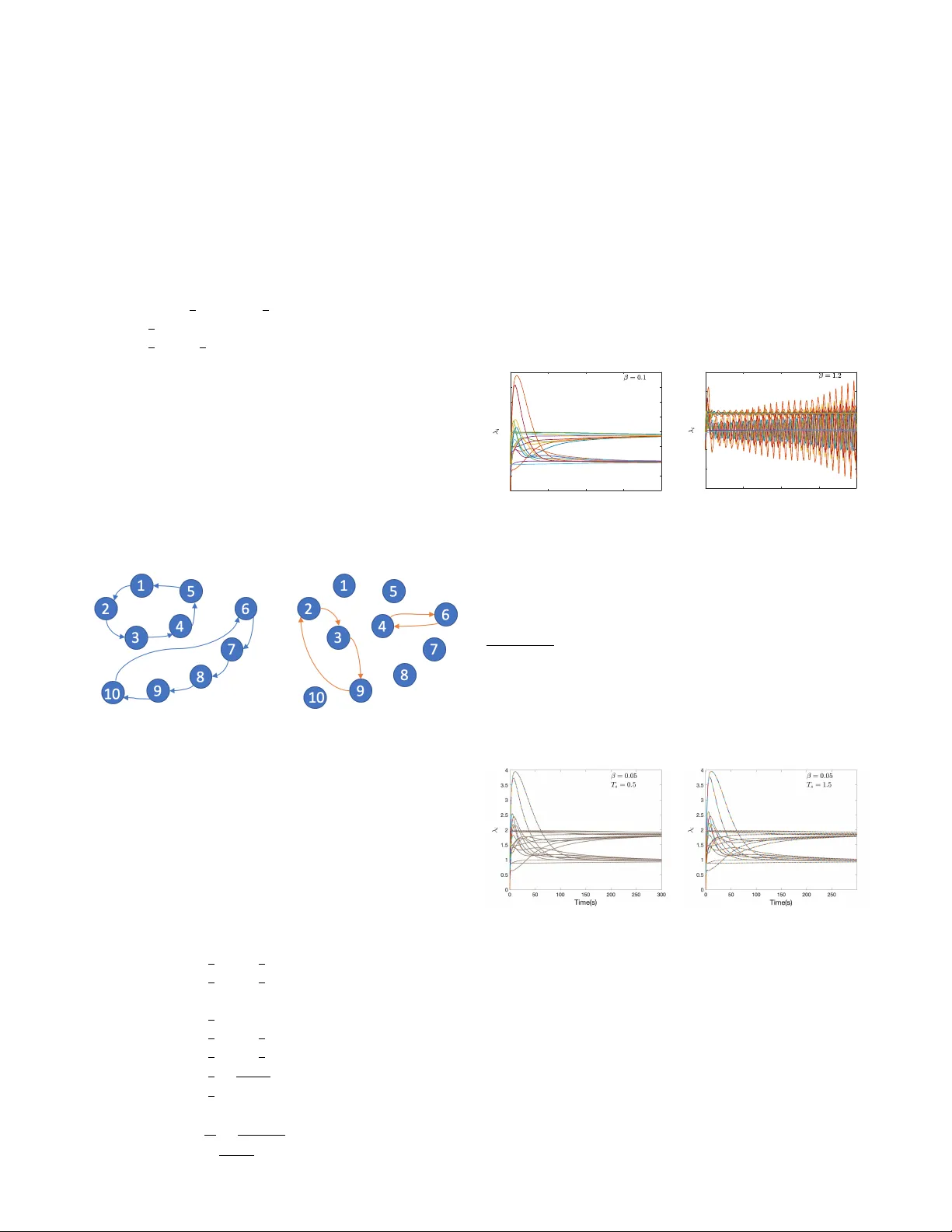
1 Distrib uted Resource Allocation o ver T ime-v arying Balanced Digraphs with Discrete-time Communication Lanlan Su, Mengmou Li, V ijay Gupta, and Graziano Chesi Abstract —This work is concer ned with the problem of dis- tributed resour ce allocation in continuous-time setting but with discrete-time communication over infinitely jointly connected and balanced digraphs. W e pr ovide a passivity-based perspective f or the continuous-time algorithm, based on which an intermittent communication scheme is developed. P articularly , a periodic communication scheme is first derived through analyzing the passivity degradation over output sampling of the distributed dynamics at each node. Then, an asynchronous distributed event- triggered scheme is further developed. The sampled-based event- triggered communication scheme is exempt from Zeno behavior as the minimum inter -event time is lower bounded by the sampling period. The parameters in the proposed algorithm r ely only on local information of each individual nodes, which can be designed in a truly distributed fashion. Index T erms —Resource Allocation, Input feed-forward Pas- sive, Time-v arying Balanced Graphs, Sampling, Event T riggering I . I N T RO D U C T I O N An important distributed optimization problem is one in which each node has access to a conv ex local cost function, and all the nodes collectively seek to minimize the sum of all the local cost functions [1]–[4]. Most optimization algorithms reported in the literature are implemented in discrete time. Howe ver , as pointed out by [5], [6], discrete-time algorithms might be insufficient for applications where the optimization algorithm is not run digitally , but rather via the dynamics of a physical system, such as collecti vely optimizing social, bio- logical and natural systems, robotic systems [7]. The resource allocation, as an important class of distributed optimization problem, has been studied in continuous-time setting [8]– [13] and discrete-time setting [14]–[16]. The e xisting w orks concerned with the distributed resource allocation problem assume topology graphs to be fixed over time and/or do not take the communication cost into account. In this work, we aim at pro viding a passivity-based perspective for a continuous- time algorithm of distributed resource allocation o ver time- varying digraphs, based on which an intermittent communica- tion scheme is dev eloped. Passi vity serves as a useful tool to analyze multi-agent systems (MASs). This has been well illustrated by [17] which L. Su is with School of Engineering, Univ ersity of Leicester, Leicester, LE1 7RH, UK (email: ls499@leicester .ac.uk); M. Li and G. Chesi are with the Department of Electrical and Electronic Engineering, Univ ersity of Hong K ong, Hong Kong (email:mmli.research@gmail.com, chesi@eee.hku.hk); V . Gupta is with Department of Electrical Engineering, Univ ersity of Notre Dame, Notre Dame, IN 46556 USA (email:vgupta2@nd.edu). shows that a MAS of possibly heterogeneous agents can reach consensus over a time-varying balanced strongly connected graph as long as all individual agents are input-output passi ve. In [18], we generalize the results of [17] to MASs with all agents that can be characterized by a passi vity index. The current work is rooted in the same idea, but we would like to note that it is not trivial to apply the idea for consensus of MASs to distributed optimization problems. One of the main challenges is to v erify that the individual algorithmic dynamics of a particular distributed algorithm is dissipative with a quantified input feed-forward passive (IFP) index. On the other hand, the passivity and dissipati vity (including IFP as a special case) hav e been recently exploited in netw orked control systems coping with different communication imperfections. For instance, [19] addresses the problem of output synchro- nization of passiv e systems with ev ent-triggered communica- tion wherein network delay and quantization are considered as well; in [20], passivity index has been used to feedback control two-dimensional systems over digital communication network wherein output sampling and e vent-triggered scheme are designed; [21] uses a passivity framework to model and mitigate attacks on networked control system; [22] considers the packet drops of the communication channel. See [23] for more recent works on cyber-physical systems using passi vity indices. This forges the main motiv ation for us to provide a passivity-based perspectiv e for the algorithm as the IFP framew ork opens up the new possibilities of implementing the algorithm ov er a nonideal digital communication network and reduce the channel usage. Whereas there exist considerable works on algorithms de- sign for distributed optimization, there are relatively fe wer works that take communication constraints into account. In this work, we are interested in intermittent communication including periodic (also called sampled-based) and ev ent- triggered manners. The underpinning distrib uted algorithms proposed in the existing works in this direction are either discrete-time [14], [15], [24]–[27] (see T ables 1 and 2 in [6] for a comprehensiv e list) or continuous-time [12], [28]–[35] (see T able 3 in [6] for a comprehensiv e list). Among the works concerned with continuous-time algorithms with a discrete- time communication scheme, the results in [12], [28], [30], [31], [33], [35] are limited to undirected and fixed topological graphs while [29], [32], [36] assume the graph to be strongly connected and fixed over time. [34] studies the problem of ev ent-triggered distributed optimization over a uniformly jointly connected graph but restricts it to be undirected. T o 2 the best of our knowledge, distributed optimization problem ov er time-varying jointly connected digraphs has nev er been addressed in the continuous-time setting due to the difficulties from stability analysis under the time-v arying nature and lack of connectedness of topologies. The passivity-based method has been shown to be powerful in handling communication imperfections and in distributed control, thus being a promis- ing approach to treat both the time-varying graph topology and communication. In this work, we consider the problem of distributed re- source allocation over a time-v arying digraph under inter- mittent communication. Specifically , each node has access to its own local cost function and local network resource, and the goal is to minimize the sum of the local cost functions subject to a global network resource constraint. The com- munication topology is described by a weight-balanced and infinitely jointly strongly connected digraph. Closest papers which have also exploited the notion of passivity to address the distributed optimization problem are [37], [38]. The results in these mentioned works are limited to fixed and undirected graphs. Our work features a novel passivity-based perspectiv e for continuous-time algorithms, which enables us to design an intermittent communication scheme over infinitely jointly strongly connected digraphs. Starting from a continuous-time algorithm, a periodic communication scheme is first deriv ed through analyzing the passivity degradation ov er output sam- pling of the distributed dynamics at each node. Then, an asynchronous distributed event-triggered scheme is further dev eloped. The sampled-based event-triggered communication scheme is exempt from Zeno behavior as the minimum inter- ev ent time is lo wer bounded by the sampling period. The parameters in the proposed algorithm rely only on local information of each indi vidual nodes, which can be designed in a truly distributed fashion. The rest of this paper is organized as follows. Section II introduces some preliminaries and states the problem formula- tion. Section III presents the main results. Specifically , Section III-A reformulates the problem into its dual distributed conv ex optimization problem. Section III-B proposes a continuous- time algorithm, and by providing a novel passivity-based per- spectiv e of the proposed algorithm, a distributed condition is provided for con vergence ov er time-varying digraphs. In III-C, a periodic communication scheme based on the passi vity-based notion is presented, and an event-triggered communication scheme is dev eloped in Section III-D. The main results are illustrated by an example in Section IV. Some final remarks and future works are described in Section V. I I . P R E L I M I NA R I E S A N D P R O B L E M F O R M U L AT I O N In this section, we first introduce our notation, some con- cepts of conv ex functions and graph theory follo wed by a passivity-related definition. Then, the problem to be addressed in this work is formulated. Notation Let R and N denote the set of of real numbers and nonnegati ve integers, respectively . The identity matrix with size m is denoted by I m . For symmetric matrices A and B , the notation A ≥ B ( A > B ) denotes A − B is positiv e semidefinite (positive definite). diag ( a i ) is the diagonal matrix with a i being the i -th diagonal entry . 0 m and 1 m denote all zero and one vectors with size m × 1 . For column vectors v 1 , . . . , v m , col ( v 1 , . . . , v m ) = ( v T 1 , . . . , v T m ) T . || λ || denotes the Euclidean norm of vector λ . Given a positiv e semidefinite matrix A ∈ R N × N , σ + min ( A ) and σ N ( A ) denote the smallest positiv e and the largest eigen value of A , respectiv ely . For a twice differentiable function f ( x ) , its gradient and Hessian are denoted by ∇ f ( x ) and ∇ 2 f ( x ) , respectiv ely . range ( ∇ f ( x )) denotes the range of the function ∇ f ( x ) . Giv en a linear map- ping L , null ( L ) denotes the null space of L . The Kronecker product is denoted by ⊗ . Con vex function A differentiable function f : R m → R ov er a con vex set X ⊂ R m is strictly conv ex if and only if ( ∇ f ( x ) − ∇ f ( y )) T ( x − y ) > 0 , ∀ x 6 = y ∈ X , and it is µ - strongly conv ex if and only if ( ∇ f ( x ) − ∇ f ( y )) T ( x − y ) ≥ µ || x − y || , ∀ x, y ∈ X , if and only if f ( y ) ≥ f ( x ) + ∇ f ( x ) T ( y − x ) + µ 2 || y − x || 2 , ∀ x, y ∈ X . A function g : R m → R m ov er a set X is l -Lipschitz if and only if || g ( x ) − g ( y ) || ≤ l || x − y || , ∀ x, y ∈ X . Algebraic graph theory A digraph is a pair G = ( I , E ) where I = 1 , . . . , N is the node set and E ⊆ I × I is the edge set. An edge ( j, i ) ∈ E means that node j can send information to node i , and i is called the out-neighbor of j while j is called the in-neighbor of i . A digraph is strongly connected if for every pair of nodes there exists a directed path connecting them. A time-varying graph G ( t ) is uniformly jointly strongly connected if there exists a constant T > 0 such that for any t k , the union ∪ t ∈ [ t k ,t k + T ] G ( t ) is strongly connected. A time- varying graph G ( t ) is infinitely jointly strongly connected if the union ∪ t ∈ [ t, ∞ ] G ( t ) is strongly connected for all t ≥ 0 . Note that infinitely jointly connected graphs are less restrictive than uniformly jointly strongly connected graphs as they do not require an upper bound for T . A weighted digraph is a triple G = ( I , E , A ) where A ∈ R N × N is a weighted adjacency matrix defined as A = [ a ij ] with a ii = 0 , a ij > 0 if ( i, j ) ∈ E and a ij = 0 , otherwise. The weighted in- degree and out-degree of node i are d i in = P N j =1 a ij and d i out = P N j =1 a j i , respectively . A digraph is said to be weight- balanced if d i in = d i out , ∀ i ∈ I . The Laplacian matrix of G is defined as L = D in − A where D in = diag ( d i in ) . Input feed-forward passive Consider the following non- linear system: H :  ˙ s = F ( s, u ) y = Y ( s, u ) , where s ∈ S ⊂ R n , u ∈ U ⊂ R m and y ∈ R m are the state, input and output variables, respectively , and S, U are the state and input spaces, respectiv ely . F and Y are state function and output function. Definition 1: ([39]) System H is Input feed-forwar d P assive (IFP) if there exists a nonnegativ e real function V ( s ) : S → R + , called the storage function, such that for all t 1 ≥ t 0 ≥ 0 , initial condition s 0 ∈ S and u ∈ U , V ( s ( t 1 )) − V ( s ( t 0 )) ≤ Z t 1 t 0 u T y − ν u T udt (1) 3 for some ν ∈ R , denoted as IFP( ν ). If the storage function V ( s ) is differentiable, the inequality (1) is equiv alent to ˙ V ( s ) ≤ u T y − ν u T u. (2) As it can be seen from the abov e definition, a positiv e value of ν means that the system has an excess of passivity while a negati ve value of ν means the system lacks passivity . The index ν can be taken as a measurement to quantify ho w passiv e a dynamic system is. This concept will play a crucial role in the subsequent results. Problem formulation Each node i has a local cost function f i ( x i ) : R m → R where x i ∈ R m is the local decision variable. The sum of f i ( x i ) is considered as the global cost function. W e make the following assumptions. Assumption 1: Each f i , i ∈ I is twice differentiable with ∇ 2 f i ( x i ) > 0 and its gradient ∇ f i ( x i ) is l i -Lipschitz. Under Assumption 1, f i is strictly con vex and ||∇ f i ( x i ) − ∇ f i ( y i ) || ≤ l i || x i − y i || . (3) Thus, its Hessian satisfies 0 < ∇ 2 f i ( x i ) ≤ l i I , ∀ i ∈ I . (4) Assumption 2: The time-varying communication graph G ( t ) is weight-balanced and infinitely jointly strongly connected. The objectiv e is to design a continuous-time distributed algorithm such that the following problem min x 1 ,...,x N N X i =1 f i ( x i ) s.t. N X i =1 x i = N X i =1 d i (5) is solved by each node using only its own information and exchanged information from its neighbors under discrete- time communication. In fact, this problem can be used to formulate many practical applications such as network utility maximization and economic dispatch in power systems. Let us denote x = col ( x 1 , . . . , x N ) . It can be observed that problem (5) is feasible and has a unique optimal point x ∗ . I I I . M A I N R E S U LT S A. The Lagrange dual pr oblem In this subsection, we show that the resource allocation problem (5) can be equiv alently conv erted into a general distributed conv ex optimization. Let us define a set of new variable λ i ∈ R m , i ∈ I , and denote the set of range ( ∇ f i ) as Λ i . It can be deriv ed from [40] that Λ i is a conv ex set. Under Assumption 1, we have that the in verse function of ∇ f i ( · ) exists and is differentiable, denoted as h i ( · ) 1 , and further define g i ( λ i ) , f i ( h i ( λ i )) + λ T i ( d i − h i ( λ i )) (6) 1 If the analytic form of the in verse function h i ( · ) can not be obtained, one can replace h i ( · ) by argmin x i { f i ( x i ) − λ T i x i } in the algorithms that will be proposed later . This replacement does not affect our analysis. when λ i ∈ Λ i . Lemma 1: Problem (5) can be equiv alently solved by the following con vex optimization min λ i ∈ Λ i , ∀ i ∈I J ( λ ) = N X i =1 J i ( λ i ) s.t. λ i = λ j , ∀ i, j ∈ I (7) with J i ( λ i ) = − g i ( λ i ) and ∇ J i ( λ i ) = h i ( λ i ) − d i . Moreover , J i ( λ i ) is twice differentiable and 1 l i -strongly con vex in the domain Λ i , i.e., 1 l i ≤ ∇ 2 J i ( λ i ) , ∀ λ i ∈ Λ i . Proof . This result can be obtained via the duality [41].  Due to the strong duality , the primal optimal solution x ∗ is a minimizer of L ( x, λ ∗ ) which is defined as L ( x, λ ∗ ) = N X i =1 f i ( x i ) + λ ∗ T N X i =1 d i − N X i =1 x i ! (8) This fact enables us to recover the primal solution x ∗ from the dual optimal solution λ ∗ . Specifically , since f i is strictly con vex, the function L ( x, λ ∗ ) is strictly con vex in x , and therefore has a unique minimizer which is identical to x ∗ . Moreov er, since L ( x, λ ∗ ) is separable according to (8), we can recov er x ∗ i from x ∗ i = h i ( λ ∗ ) . Based on Lemma 1, we then aim to design an continuous- time algorithm for problem (7). For simplicity , we will abuse the notation by using λ = col ( λ 1 , . . . , λ N ) hereafter . B. IFP-based Distributed Algorithm Design For i ∈ I and with constant scalars α, β > 0 , let us consider the following continuous-time algorithm ˙ λ i = − α ( h i ( λ i ) − d i ) − γ i ˙ γ i = − u i u i = β P N j =1 a ij ( t )( λ j − λ i ) (9) where λ i , γ i ∈ R m are the local states variables and u i ∈ R m is the local input. α > 0 is a predefined constant and β > 0 is the coupling gain to be designed. A ( t ) = [ a ij ( t )] N × N is the adjacency matrix of the graph G ( t ) . Let γ = col ( γ 1 , . . . γ N ) , d = col ( d 1 , . . . , d N ) and h ( λ ) = col ( h 1 ( λ 1 ) , . . . , h N ( λ N )) . The algorithm (9) can be rewritten in a compact form as ˙ λ = − α ( h ( λ ) − d ) − γ ˙ γ = β L ( t ) λ (10) where L ( t ) = L ( t ) ⊗ I m with L ( t ) being the Laplacian matrix of the graph G ( t ) . The abov e continuous-time algorithm is a simplification of the one proposed in [28] which is moti vated by the feedback control consideration. Specifically , each node ev olves in the direction of gradient decent while trying to reach an agreement with its neighbors. T o correct the error between the local gra- dient and the consensus with neighbors, the integral feedback of u i representing the node disagreements is exploited. An important reason for using such an algorithm is that it enables 4 us to provide a passivity-based perspectiv e for the individual algorithmic dynamics later . In the rest of this work, we assume that λ i (0) ∈ Λ i for all i ∈ I . This can be tri vially satisfied by letting λ i (0) = ∇ f i ( x i (0)) . In the following, we will first show in Lemma 2 that the optimal solution of (7) coincides with the equilibrium point of algorithm (9). Then we provide a passi vity-based perspecti ve for the error dynamics in each indi vidual node in Theorem 1, based on which the con vergence of algorithm (9) is sho wn in Theorem 2. Lemma 2: Under Assumptions 1 and 2, the equilibrium point ( λ ∗ , γ ∗ ) of the system (9) with the initial condition P N i =1 γ i (0) = 0 is unique and λ ∗ is the optimal solution of problem (7). Proof . Suppose ( λ ∗ , γ ∗ ) is the equilibrium of system (9) and P N i =1 γ i (0) = 0 . It follows that ˙ λ ∗ = − α ( h ( λ ∗ ) − d ) − γ ∗ = 0 ˙ γ ∗ = β L ( t ) λ ∗ = 0 . (11) Since (1 N ⊗ I m ) T L ( t ) = 0 T N m , we hav e (1 N ⊗ I m ) T ˙ γ = β (1 N ⊗ I m ) T L ( t ) λ = 0 , which giv es P N i =1 ˙ γ i = 0 . Hence, it can be observed that P N i =1 γ i ( t ) = P N i =1 γ i (0) = 0 m for any t ≥ 0 . Next, let us multiply (1 N ⊗ I m ) T from the left of the ˙ λ ∗ , and obtain that (1 N ⊗ I m ) T ˙ λ ∗ = − α (1 N ⊗ I m ) T ( h ( λ ∗ ) − d ) − P N i =1 γ ∗ i = 0 , which indicates that ∇ J ( λ ∗ ) = N X i =1 ∇ J i ( λ ∗ i ) = N X i =1 ( h i ( λ ∗ i ) − d i ) = 0 . Moreov er, since the graph G ( t ) is infinitely jointly strongly connected, ˙ γ ∗ = β L ( t ) λ ∗ ≡ 0 implies that λ ∗ 1 = . . . = λ ∗ N . Under Assumption 1, problem (7) has a unique solution, which coincides with λ ∗ based on the optimality condition [42].  Before proceeding to show in Theorem 2 that the algorithm con verges, let us inv estigate the IFP property of the error dynamics in each individual node. Denote ∆ λ i = λ i − λ ∗ i and ∆ γ i = γ i − γ ∗ i . Comparing (9) and (11) yields the individual error system shown as Ψ i :    ∆ ˙ λ i = − α ( h i ( λ i ) − h i ( λ ∗ i )) − ∆ γ i ∆ ˙ γ i = − u i u i = β P N j =1 a ij ( t )(∆ λ j − ∆ λ i ) . (12) By taking u i and ∆ λ i as the input and output of the error system Ψ i , the follo wing theorem sho ws that each error system Ψ i is IFP with the proof provided in Appendix. Theor em 1: Suppose Assumption 1 holds. Then, the system Ψ i is IFP( ν i ) from u i to ∆ λ i with ν i ≥ − l 2 i α 2 . Remark 1: It is shown in the above theorem that for the nonlinear system (12) resulting from general strongly conv ex objectiv e function J i ( λ i ) is IFP from u i to ∆ λ i . Moreover , the IFP index is lower bounded by − l 2 i α 2 , which means that the system (12) can have the IFP index arbitrarily close to 0 (i.e, passivity) if the coefficient α can take arbitrarily large v alue. Howe ver , it might be impractical to choose an infinitely large α due to the potential numerical error or larger computing costs when solving the ordinary differential equation (10) numerically . In view of this, in order to achie ve larger IFP index, we can choose α as the largest positiv e number allowed by the error tolerance error lev el of the available computing platform. It is worth mentioning that similar algorithm with (9) has been shown in [28]. The contribution of Theorem 1 is to provide a novel passivity-based perspectiv e of the proposed algorithm, and this perspecti ve will lead to fruitful results in the remainder of this section. The next theorem provides a condition to design the cou- pling gain β under which the algorithm (9) will con verge to the optimal solution of problem (7). Theor em 2: Under Assumptions 1 and 2, suppose the coupling gain β satisfies 0 < β < α 2 σ + min  L ( t ) + L ( t ) T  2 σ N ( L ( t ) T diag ( l 2 i ) L ( t )) , (13) where σ + min and σ N are the smallest positi ve and the largest eigen value respectiv ely . Then under algorithm (9), for all i ∈ I , the set Λ i is a positively in variant set of λ i , and the algorithm (9) with any initial condition with P N i =1 γ i (0) = 0 will con verge to the optimal solution of (7). Proof . The proof is stated in Appendix.  Remark 2: Lemma 2 states that the equilibrium point of the continuous-time algorithm (9) under the initial constraint P N i =1 γ (0) = 0 is identical to the optimal solution of the distributed optimization problem (7) while Theorem 2 states that the algorithm (9) will conv erge to such an equilibrium point if the coefficients α and β are chosen to satisfy (13). As discussed in Section III-A, the optimal solution x ∗ i of the original resource allocation problem (5) can be recovered from x ∗ i = h i ( λ ∗ ) . In this view , the distributed algorithm in (9) utilizes only local interaction with exchanging λ i instead of the real decision v ariable x i to achie ve the optimal collectiv e goal. It should be mentioned that the condition proposed in Theorem 2 maybe dif ficult to be examined in a time-v arying graph. Ne v- ertheless, the follo wing distributed condition can be obtained based on Theorem 2. Cor ollary 1: Under Assumptions 1 and 2, the algorithm (9) with any initial condition with P N i =1 γ i (0) = 0 will con verge to the optimal solution of (7) if the coupling gain β > 0 satisfies : β l 2 i α 2 d i in ( t ) < 1 2 , ∀ i ∈ I , ∀ t > 0 (14) where d i in ( t ) denotes the in-degree of the i -th node. Proof . The proof is stated in Appendix.  Remark 3: (Design of parameter β ) In order to implement the algorithm (9), the parameter β needs to be designed. The condition proposed in the above corollary provides a distributed strategy to design β . A heuristic solution is to let 5 each node compute the maximum β according to (14) and search the minimum of β among them by communicating among neighboring nodes. Repeat this procedure when a smaller β is updated (a larger d i in ( t ) is detected) at any node due to the graph variation. Howe ver , this has to be done in an off-line manner . A possible more easy way is to let the upper bound of β be α 2 2 max i { l i } ( N − 1) when a ij ≤ 1 , ∀ i, j . C. P eriodic Discr ete-time Communication Continuous-time communication among the nodes is re- quired in the distrib uted algorithm proposed in Section III-B whereas a digital network with limited channel capacity gener- ally allows communication only at discrete instants. Moreover , the communication cost is far larger than the computation cost in real applications like sensor networks [43]. T o separate the communication and the computation, we will in vestigate in this subsection the distributed algorithm design under periodic discrete-time communication by exploiting the IFP property stated in Theorem 1. By considering a sampling based scheme, we proceed to in vestigate the conv ergence of algorithm (9) with periodic communication. Fig. 1. Sampled continuous distributed algorithm. As depicted in Figure 1, let us consider the algorithm with sampling at each output of individual node, ˙ λ i = − α ( h i ( λ i ) − d i ) − γ i ˙ γ i = − u i ¯ u i ( k ) = β P N j =1 a ij ( k )( ¯ λ j ( k ) − ¯ λ i ( k )) (15) where a ij ( k ) denotes a ij ( t ) at the k -th sampling instant, the output ¯ λ i is obtained by sampling the continuous-time output λ i , while the input u i depending on the sampled ¯ λ i , ∀ i ∈ I i is applied to the continuous-time system through a zero order holder . In particular , let the sampling period be denoted as T s , and then for all k ∈ N , ¯ λ i ( k ) = λ i ( k T s ) , u i ( t ) = ¯ u i ( k ) , ∀ t ∈ [ k T s , ( k + 1) T s ) . (16) Since the communication is carried out in periodic discrete- time instants, we need to make the following additional assumption for the graph. Denote the time sequence k = { 0 , T s , 2 T s , . . . } . Assumption 3: The time-varying graph G ( k ) is balanced and infinitely jointly strongly connected, i.e., there exists an unbounded time sequence k , k + 1 , k + 2 , . . . such that G ( k ) ∪ G ( k + 1) ∪ G ( k + 2) ∪ · · · is strongly connected for any k ∈ N . W ith ∆ ¯ λ i = ¯ λ i − λ ∗ i where λ ∗ i is defined in (11), the error dynamics of subsystem i is ¯ Ψ i :    ∆ ˙ λ i = − α ( h i ( λ i ) − h i ( λ ∗ )) − ∆ γ i ∆ ˙ γ i = − u i ¯ u i = β P N j =1 a ij (∆ ¯ λ j − ∆ ¯ λ i ) . (17) In the follo wing, we first analyze and approximate the bound of the sampling error ∆ λ i − ∆ ¯ λ i with respect to the input ¯ u i in Lemma 3 and 4. Based on these results, Theorem 3 characterizes the passivity degradation over sampling of the error dynamics at each node, and the con vergence of the algorithm (15) is stated in Corollary 2. For notational simplicity , let us denote z i = ∆ ˙ λ i . Lemma 3: Suppose Assumption 1 holds. Then, under the dynamics ¯ Ψ i , it holds that for all u i ∈ R m , l i α · d || z i || 2 dt ≤ l 2 i α 2 || u i || 2 − || z i || 2 . (18) Proof . The deriv ativ e of z i yields that ˙ z i = − α ∂ h i ( λ i ) ∂ λ i z i − ∆ ˙ γ i = − α ∂ h i ( λ i ) ∂ λ i z i + u i and it leads to l i α · d || z i || 2 dt = 2 l i α z T i  − α ∂ h i ( λ i ) ∂ λ i z i + u i  . W e can also observe that 2 α l i l i α − 1 − l i α − l i α l 2 i α 2 ! ≥ 0 , which follows that  z i u i  T 2 α l i l i α − 1 − l i α − l i α l 2 i α 2 ! ⊗ I m !  z i u i  ≥ 0 , ∀ z i , u i . Since 1 l i I m ≤ ∂ h i ( λ i ) ∂ λ i under Assumption 1, we further obtain that for all z i , u i ∈ R m  z i u i  T 2 l i α  α ∂ h i ( λ i ) ∂ λ i  − I m − l i α I m − l i α I m l 2 i α 2 I m !  z i u i  ≥ 0 , which is equiv alent to l i α d || z i || 2 dt ≤ l 2 i α 2 || u i || 2 − || z i || 2 .  From the above lemma, it can be seen by the integration of (18) ov er t ∈ [ k T s , ( k + 1) T s ] that l i α || z i (( k + 1) T s ) || 2 − l i α || z i ( k T s ) || 2 ≤ l 2 i α 2 R ( k +1) T s kT s || u i ( t ) || 2 dt − R ( k +1) T s kT s || z i ( t ) || 2 dt. (19) It can be seen from the form of (18) or (19) that l 2 i α 2 provides the upper bound of the L 2 gain for the mapping u i → z i since the specific form of storage function, l i α || z i || 2 , is considered. Lemma 4: Under Assumption 1, for all k ∈ N , the following inequality holds R ( k +1) T s kT s || ∆ λ i ( t ) − ∆ ¯ λ i ( k ) || 2 dt ≤ T 2 s ·  T s l 2 i α 2 || ¯ u i ( k ) || 2 + l i α  || z i ( k T s ) || 2 − || z i (( k + 1) T s ) || 2   . (20) 6 Proof . First, let us observe that for all t ∈ [ k T s , ( k + 1) T s ) , ∀ k ∈ N ,         Z t kT s ∆ ˙ λ i ( s ) ds         2 ≤           Z ( k +1) T s kT s       ∆ ˙ λ i ( s )       ds           2 ≤ T s Z ( k +1) T s kT s       ∆ ˙ λ i ( s )       2 ds (21) where the second inequality holds based on Cauchy-Schwarz inequality . Next, it follows from (19) and (21) that R ( k +1) T s kT s || ∆ λ i ( t ) − ∆ ¯ λ i ( k ) || 2 dt = R ( k +1) T s kT s || R t kT s ∆ ˙ λ i ( s ) ds || 2 dt ≤ R ( k +1) T s kT s  T s R ( k +1) T s kT s       ∆ ˙ λ i ( s )       2 ds  dt = T 2 s R ( k +1) T s kT s       ∆ ˙ λ i ( s )       2 ds ≤ T 2 s l 2 i α 2 R ( k +1) T s kT s || u i ( s ) || 2 ds + T 2 s l i α ·  || z i ( k T s ) || 2 − || z i (( k + 1) T s ) || 2  . Based on the relationship between u i ( t ) and ¯ u i ( k ) shown in (16), the inequality (20) can be therefore obtained.  Theor em 3: Under Assumption 1, the sampled system ¯ Ψ i is IFP ( ¯ ν i ) from ¯ u i to ∆ ¯ λ i with ¯ ν i ≥ −  l 2 i α 2 + T s l i α  where T s is the sampling period. Proof . The proof is stated in Appendix.  Theorem 3 shows that the lower bound of the IFP index, ν , decreases from − l 2 i α 2 to − l 2 i α 2 − T s l i α ov er the sampling. This passivity ”degradation” is caused by sampling error , which depends on the sampling period T s . Based on this new IFP index bound, a revised distrib uted condition for conv ergence of the algorithm (15) is provided as follows. Cor ollary 2: Under Assumptions 1 and 3, the algorithm (15) under periodic communication with any initial condition with P N i =1 γ i (0) = 0 will con verge to the optimal solution of (7) if the following condition is satisfied for all t ≥ 0 : β  l 2 i α 2 + T s l i α  d i in ( t ) < 1 2 , ∀ i ∈ I . (22) Proof . This condition can be deriv ed based on similar argument in the proofs of Theorem 2 and Corollary 1, and the discrete-time LaSalle’ s inv ariance principle [44].  As shown in the above corollary , when α and β are fixed and satisfy the condition (14), there always exists a constant T s > 0 satisfying (22). Indeed, with fixed α and β , the sampling period T s can also be determined in a distributed way by a similar heuristic solution described in Remark 3. It is worth noting that a sufficiently large sampling period T s is acceptable provided α is large enough and coupling gain β is small enough. D. Distributed Event-Driven Communication Build on the sampled-based framework in the preceding subsection, we further consider an ev ent-driv en communi- cation strategy . Reconsider the algorithm as shown in (15) Fig. 2. Continuous distributed algorithm with sampled-based e vent-triggered communication. by incorporating an ev ent-driven communication mechanism depicted by Figure 2, i.e., ˙ λ i = − α ( h i ( λ i ) − d i ) − γ i ˙ γ i = − u i ˆ u i ( k ) = β P N j =1 a ij ( k )( ˆ λ j ( k ) − ˆ λ i ( k )) (23) where ˆ λ i ( k ) , i ∈ I denotes the last known state of node i that has been transmitted to its neighbors at the time kT s . Similar to (16), we set ¯ λ i ( k ) = λ i ( k T s ) , u i ( t ) = ˆ u i ( k ) , ∀ t ∈ [ k T s , ( k + 1) T s ) . (24) The following theorem presents a triggering condition for each node to update its output while the con vergence to the global optimal solution is ensured. Theor em 4: Under Assumptions 1 and 3, consider the algorithm (23). If α, β are designed such that (22) holds, and the triggering instant for node i, i ∈ I to transmit its current information of λ i is chosen whenev er the following condition is satisfied k e i ( k ) k 2 ≥ c i d i in ( k )  1 2 − β d i in ( k )  l 2 i α 2 + T s l i α  2 · N X j =1 a ij ( k ) k ˆ λ j ( k ) − ˆ λ i ( k ) k 2 (25) where e i ( k ) = ¯ λ i ( k ) − ˆ λ i ( k ) and c i ∈ (0 , 1) , then the algorithm (23) with any initial condition with P N i =1 γ i (0) = 0 will con verge to the optimal solution of (7). Proof . The proof is stated in Appendix.  Under the ev ent triggering condition (25), each node broad- casts its current state (after sampling) ¯ λ i ( k ) to its out- neighbors when a local “error” signal exceeds a threshold depending on its own cost function and the last received state of ˆ λ j ( k ) from its in-neighbors. Such an triggering condition requires each node being aw are of the existence of its in- neighbors. Whenever an edge between two nodes is estab- lished, the sender sends its last triggered state to the receiver , which is not considered as a “triggering”. Whenever an edge is canceled or established, the receiver updates its input ˆ u i ( k ) by removing or adding the corresponding item of ˆ λ . Remark 4: Given fixed α, β and T s , condition (25) is a simple and distributed one to be verified by each node ov er a balanced graph with very weak connecti vity (Assumption 2). 7 It is worth mentioning that this sampled-based ev ent-triggered communication scheme is ex empt from Zeno behavior as the minimum inter-e vent time can be guaranteed by the sampling period T s . I V . S I M U L AT I O N In this section, a numerical example is provided to illustrate the previous results. Consider the resource allocation problem (5) with N = 10 , m = 2 , and f 1 ( x 1 ) = x 2 11 + 1 2 x 11 x 12 + 1 2 x 2 12 + 1; f 2 ( · ) = f 1 ( · ); f 3 ( x 3 ) = 1 4 ( x 31 + 2) 2 + x 2 32 ; f 4 ( · ) = f 3 ( · ); f 5 ( x 5 ) = 1 2 x 2 51 − 1 2 x 51 x 52 + x 2 52 ; f 6 ( · ) = f 5 ( · ); f 7 ( x 7 ) = ln( e 2 x 71 + 1) + x 2 72 ; f 8 ( · ) = f 7 ( · ); f 9 ( x 9 ) = ln( e 2 x 91 + e − 0 . 2 x 91 ) + ln( e x 92 + 1); f 10 ( · ) = f 9 ( · ) . and d 1 = d 2 = d 3 = d 4 = d 5 = [1 1] T , d 6 = d 7 = d 8 = d 9 = d 10 = [2 2] T . Suppose the communication graph G ( t ) is time varying, which alternates ev ery 1s between G 1 and G 2 shown in Fig. 2. It can be observed that the switching graph G ( t ) is weight-balanced and infinitely jointly strongly connected, and Assumption 1 holds with l 1 = l 2 = l 5 = l 6 = 2 . 21 , l 3 = l 4 = 1 7 = l 8 = 2 , l 9 = l 10 = 1 . 21 . Fig. 3. The switching communication graph G ( t ) . W e solve the centralized conv ex problem (5) using Y almip, and obtain the optimal solution x ∗ i , i = 1 , . . . , 10 . According to Lemma 1, λ ∗ 1 = . . . = λ ∗ 10 = ∇ f i ( x ∗ i ) = [1 . 87 0 . 992] T . The goal is to design a continuous-time distributed algorithm to equiv alently solve the optimization problem (5) under discrete- time communication. T o start with, we recast the above problem into (7) based on Section III-A. It can be obtained that ∆ J i ( λ i ) = h i ( λ i ) − d i with h 1 ( λ 1 ) =  4 7 λ 11 − 2 7 λ 12 8 7 λ 12 − 2 7 λ 11  ; h 2 ( · ) = h 1 ( · ); h 3 ( λ 3 ) =  2 λ 31 − 2 1 2 λ 32  ; h 4 ( · ) = h 3 ( · ) h 5 ( λ 5 ) =  8 7 λ 51 + 2 7 λ 52 2 7 λ 51 + 4 7 λ 52  ; h 6 ( · ) = h 5 ( · ); h 7 ( λ 7 ) =  1 2 ln λ 71 2 − λ 71 1 2 λ 72  ; h 8 ( · ) = h 7 ( · ); h 9 ( λ 9 ) = 5 11 ln 5 λ 91 +1 10 − 5 λ 91 ln λ 91 1 − λ 91 ! ; h 10 ( · ) = h 9 ( · ) . In the following simulations, we fix α = 1 , and fix γ i (0) = 0 , ∀ i ∈ I to satisfy the initial condition P N i =1 γ i (0) = 0 . T o examine the effecti veness of the distributed algorithms amounts to checking whether the trajectories of λ i ( t ) , i ∈ I con verge to the value λ ∗ = [1 . 87 0 . 992] T . Let us first implement the distributed algorithm (9) under continuous communication. By the condition (14) in Corollary 1, one has that the algorithm (10) will con verge with 0 < β < 0 . 103 . Under randomly generated initial value of x i (0) , the trajectories of λ i ( t ) , i ∈ I are shown in Figure 4 with different value of β . Although condition (14) is only sufficient, it is shown in Figure 4 that the conv ergence is no longer ensured when β takes some larger v alue. 0 50 100 150 200 Time(s) 0 0.5 1 1.5 2 2.5 3 3.5 4 (a) 0 50 100 150 200 Time(s) -2 -1 0 1 2 3 4 (b) Fig. 4. Trajectories of λ i ( t ) under continuous communication. Next, we explore the distributed algorithm (15) under pe- riodic communication. By exploiting the condition (22), we hav e that the algorithm (15) will con verge with 0 < β < 1 9 . 74+4 . 41 T s . If we let β = 0 . 05 , then the condition yields that T s < 2 . 3 . In this example, we let T s = 0 . 5 , 1 . 5 and it is obvious that Assumption 3 holds. The trajectories of λ i ( t ) are shown in Figure 5. Note that the T s here is relativ ely large such that communication is greatly reduced. (a) (b) Fig. 5. Trajectories of λ i ( t ) under periodic communication. In the end, let us illustrate the distributed algorithm (23) under sample-based ev ent-triggered communication. W e select β = 0 . 09 , T s = 0 . 1 and c i = 0 . 5 in (25). The trajectories and the triggering instants of λ i ( t ) are shown in Figure 6. In Figure 6(b), the largest number of triggering times is 337 for node 5 while the smallest one is only 13 for node 9 and node 10 , both of which are a lot smaller than the number of periodic sampling times 300 /T s = 3000 . These shows that the sample-based event-triggered control effecti vely reduces com- munication costs. Moreover , a better con vergence performance 8 is observed in Figure 6(a) than the one in Figure 5(a) with less triggering times, due to the larger coupling gain β . (a) 0 50 100 150 200 250 300 Time (s) 0 1 2 3 4 5 6 7 8 9 10 (b) Fig. 6. T rajectories and and triggering instants of λ i ( t ) under sample-based ev ent-triggered communication. V . C O N C L U S I O N W e hav e introduced the passivity-based perspective for the continuous-time algorithm addressing the distributed resource allocation problem ov er weight-balanced and infinitely jointly connected digraphs. By showing that the individual algorith- mic dynamics is IFP , it is shown ho w to redesign the algorithm with intermittent communication protocol. The passivity-based analysis in this work is based on an existing algorithm that considers the distributed optimization without set constraints and with strong assumptions on cost functions. An interesting future direction is to inv estigate the passivity property for more advanced algorithms and apply it to time-varying graphs. Another promising direction is to explore the compatibility of the passivity-based approach with other network-induced imperfections such as time delay and packet drops. A P P E N D I X P RO O F O F T H E O R E M 1 Since the Jacobian of h i ( λ i ) satisfies 1 l i I ≤ ∂ h i ( λ i ) ∂ λ i , it follows from Mean V alue Theorem that h i ( λ i ) − h i ( λ ∗ i ) = B λ i ( λ i − λ ∗ i ) where B λ i is a symmetric λ i -dependent matrix defined as B λ i = R 1 0 ∂ h i ∂ λ i ( λ i + t ( λ i − λ ∗ i )) dt and 1 l i I ≤ B ( λ i ) . Therefore, the system (12) can be rewritten as    ∆ ˙ λ i = − αB λ i ∆ λ i − ∆ γ i ∆ ˙ γ i = − u i u i = β P N j =1 a ij ( t )(∆ λ j − ∆ λ i ) . Consider the storage function V i = η i 2 || ∆ ˙ λ i || 2 − ∆ λ T i ∆ γ i + α ( J i ( λ ∗ i ) − J i ( λ i ) + ( h i ( λ ∗ ) − d i ) T ∆ λ i ) (26) where η i is chosen to satisfy η i > l i α . First, let us verify the positive definiteness of V i . It can be observ ed that η i 2 || ∆ ˙ λ i || 2 = η i 2 || αB λ i ∆ λ i + ∆ γ i || 2 , and the strong con vexity of J i ( λ i ) provides that J i ( λ ∗ i ) − J i ( λ i ) ≥ − ( h i ( λ i ) − d i ) T ∆ λ i + 1 2 l i || ∆ λ i || 2 , which follows that the last term in the storage function V i (26) satisfies α  J i ( λ ∗ i ) − J i ( λ i ) + ( h i ( λ ∗ i ) − d i ) T ∆ λ i  ≥ α  − ( h i ( λ i ) − h i ( λ ∗ i )) T ∆ λ i + 1 2 l i || ∆ λ i || 2  = ∆ λ T i  − αB λ i + α 2 l i I  ∆ λ i . It can be deriv ed that V i ≥ η i 2 || αB λ i ∆ λ i + ∆ γ i || 2 − ∆ λ T i ∆ γ i +( α 2 l i I − αB λ i ) || ∆ λ i || 2 =  ∆ λ i ∆ γ i  T α 2 η i 2 B 2 λ i − αB λ i + α 2 l i I ∗ αη i 2 B λ i − 1 2 I η i 2 I ! | {z } W  ∆ λ i ∆ γ i  . (27) Since η i 2 I > 0 , η i > l i α and α 2 η i 2 B 2 λ i − αB λ i + α 2 l i I −  αη i 2 B λ i − 1 2 I   η i 2 I  − 1  αη i 2 B λ i − 1 2 I  = − 1 2 η i I + α 2 l i I > 0 , it can be concluded based on Schur Complement Lemma that W > 0 . Therefore, it can be claimed that V i ≥ 0 and V i = 0 if and only if ( λ i , γ i ) = ( λ ∗ i , γ ∗ i ) . The next step is to show that with the defined storage function V i , the system Ψ i is IFP( ν i ) from u i to ∆ λ i . Let us observe that η i 2 · d || ∆ ˙ λ i || 2 dt = η i ∆ ˙ λ T i  − α dh i ( λ i ) dt − ∆ ˙ γ i  = η i ∆ ˙ λ T i  − α ∂ h i ( λ i ) ∂ λ i ∆ ˙ λ i + u i  ≤ − η i α l i || ∆ ˙ λ i || 2 + η i ∆ ˙ λ T i u i , d ( − ∆ λ T i ∆ γ i ) dt = − ∆ ˙ λ T i ∆ γ i + ∆ λ T i u i . Recall that ∇ J i ( λ i ) = h i ( λ i ) − d i , and it follows α · d  J i ( λ ∗ i ) − J i ( λ i ) + ( h i ( λ ∗ i ) − d i ) T ∆ λ i  dt = α ( −∇ J i ( λ i ) + ( h i ( λ ∗ i ) − d i )) T ∆ ˙ λ i = − ( αB λ i ∆ λ i ) T ∆ ˙ λ i . By combining the abov e equations, one has that ˙ V i = η i 2 · d || ∆ ˙ λ i || 2 dt + d ( − ∆ λ T i ∆ γ i ) dt + α · d  J i ( λ ∗ i ) − J i ( λ i ) + ( h i ( λ ∗ i ) − d i ) T ∆ λ i  dt ≤ − η i α l i || ∆ ˙ λ i || 2 + η i ∆ ˙ λ T i u i + ∆ λ T i u i − ( αB ( λ i )∆ λ i + ∆ γ i ) T ∆ ˙ λ i =  − η i α l i + 1  || ∆ ˙ λ i || 2 + η i ∆ ˙ λ T i u i + ∆ λ T i u i (28) with − η i α l i + 1 < 0 . Since  − η i α l i + 1  || ∆ ˙ λ i || 2 + η i ∆ ˙ λ T i u i ≤ η 2 i 4  η i α l i − 1  u T i u i , it follows that ˙ V i ≤ ∆ λ T i u i + η 2 i 4  η i α l i − 1  u T i u i . 9 Finally , let us prov e ν i ≥ − l 2 i α 2 . T o this end, consider the following optimization problem min η i > l i α η 2 i 4  η i α l i − 1  , and it can be verified that the optimal solution is giv en by η ∗ i = 2 l i α and the corresponding minimum value of the abov e objectiv e function is l 2 i α 2 . Thus, it can be summarized that ˙ V i ≤ ∆ λ T i u i + l 2 i α 2 u T i u i , which completes the proof. P RO O F O F T H E O R E M 2 Recall the storage function defined in (26) for individual system, and consider the L yapunov function V = P N i =1 V i for the ov erall distributed algorithm. Denote u = col ( u 1 , . . . , u N ) , ∆ λ = col (∆ λ 1 , . . . , ∆ λ N ) , and it follows from (12) that u = − β ( L ( t ) ⊗ I m ) ∆ λ . Based on the result in Theorem 1, one has ˙ V ≤ P N i =1 ∆ λ T i u i + l 2 i α 2 u T i u i = − β ∆ λ T ( L ( t ) ⊗ I m ) ∆ λ + β 2 ∆ λ T  L ( t ) T ⊗ I m  ×  diag  l 2 i α 2  ⊗ I m  ( L ( t ) ⊗ I m ) ∆ λ = ∆ λ T ( M ⊗ I m ) ∆ λ with M = − β 2  L ( t ) + L ( t ) T  + β 2  L ( t ) T diag  l 2 i α 2  L ( t )  . Since a weight-balanced digraph G is strongly connected if and only if it is weakly connected (Lemma 1 in [17]), any weight-balanced digraph amounts to the union of a set of strongly connected balanced graphs. For a strongly connected balanced graph, it is apparent that its Laplacian L has the same null space with L T , which is span { 1 N } . Then, for a weight-balanced digraph, its Laplacian L and L T hav e the same null space. Therefore, Null ( L ( t ) + L ( t ) T ) is the same with Null ( L ( t ) T diag  l 2 i  L ( t )) at any time t . Besides, since G ( t ) is weight-balanced for all t , it can be easily verified that L ( t ) + L ( t ) T ≥ 0 and L ( t ) T diag  l 2 i  L ( t ) ≥ 0 . Since the abov e two matrices are both positi ve semi-definite and ha ve the same null space, it can be implied from the min-max theorem that if the condition in (13) holds, then α 2  L ( t ) + L ( t ) T  ≥ 2 β L ( t ) T diag  l 2 i  L ( t ) . (29) Thus, it can be concluded that M ≤ 0 , which leads to ˙ V ≤ 0 . Note that at any time t, M has the same null space with L ( t ) ’ s, so ˙ V ( t ) = 0 only if the nodes belonging to the same strongly connected subgraph reach output consensus. According to LaSalle’ s in variance principle, the trajectory ∆ λ tends to the largest in variant set of { ∆ λ | ˙ V ( t ) = 0 } . Moreov er, since the graph G ( t ) is infinitely jointly strongly connected, one has that ∆ λ will con verge to the set { ∆ λ | ∆ λ 1 = . . . = ∆ λ N } . According to (27), V ≥ 0 and V is radially unbounded, i.e., V → ∞ as || (∆ λ T , ∆ γ T ) T || → ∞ . Since ˙ V ≤ 0 , then V is non-increasing, and the state is bounded, i.e., λ , γ are bounded. Let us recall that Λ i , range ( ∇ f i ( x i )) with x i ∈ R m , and h i ( ∇ f i ( x i )) = x i . Let ¯ Λ i be the boundary of the set Λ i . Since x i ∈ R m is unbounded in our Problem (5) and f i is strictly con vex, then || h i ( λ i ) || → ∞ when λ i → ¯ Λ i . From the first line of (9), this yields that || ˙ λ i || → ∞ when λ i → ¯ Λ i since γ i is bounded. Consequently , based on (26), V → ∞ , which contradicts the fact that V is non-increasing. Therefore, for all i ∈ I , the set Λ i is a positiv ely in variant set of λ i . Next, let us sho w that ˙ V = 0 ⇒ ∆ ˙ λ 1 = . . . = ∆ ˙ λ N = 0 . Since the inequality in (13) is strict, it follows that there exists a small enough scalar  > 0 such that 0 < β < α 2 σ + min ( L ( t ) + L ( t ) T ) 2 σ N ( L ( t ) T diag ( l 2 i +  ) L ( t )) . (30) By substituting η i with η ∗ i = 2 l i α in (28), we hav e ˙ V i ≤ −|| ∆ ˙ λ i || 2 + 2 l i α ∆ ˙ λ T i u i + ∆ λ T i u i . By completing the square, we further have −|| ∆ ˙ λ i || 2 + 2 l i α ∆ ˙ λ T i u i ≤ −  ( l 2 i /α 2 +  ) || ∆ ˙ λ i || 2 +  l 2 i α 2 +   u T i u i . Hence, ˙ V i ≤ −   l 2 i α 2 +   || ∆ ˙ λ i || 2 +  l 2 i α 2 +   u T i u i + ∆ λ T i u i . (31) Hence, by similar argument before, it follows that ˙ V ≤ ∆ λ T  ˆ M ⊗ I m  ∆ λ − P N i =1  ( l 2 i /α 2 +  ) || ∆ ˙ λ i || 2 where ˆ M = − β 2  L ( t ) + L ( t ) T  + β 2 L ( t ) T diag  l 2 i α 2 +   L ( t ) and ˆ M ≤ 0 . As a consequence, it can be concluded that ˙ V ≤ 0 and ˙ V = 0 only if ∆ ˙ λ 1 = . . . = ∆ ˙ λ N = 0 . Because of the LaSalle’ s in variance principle, we hav e that ∆ ˙ λ → 0 and ∆ λ → 1 N ⊗ s for some s ∈ R m as t → ∞ . Furthermore, by (12), one has ∆ ˙ γ → 0 as t → ∞ . Thus, the states λ, γ under the algorithm (9) will conv erge to an equilibrium point. W ith the initial condition P N i =1 γ i (0) = 0 , it follows from Lemma 2 that the algorithm (9) will con ver ge to the optimal solution of the problem (7). P RO O F O F C O R O L LA RY 1 Define a vector variable x = col ( x 1 , . . . , x N ) T ∈ R mN and it can be observed that x T ( L ( t ) + L ( t ) T ) x ( t ) = 2 P N i =1 x i P N j =1 a ij ( t )( x i − x j ) = P N i =1 P N j =1 a ij ( t )( x i − x j ) 2 where the second equality follows from the balance of the graph G ( t ) . Suppose the condition (14) holds, i.e., α 2 > 2 β 2 l 2 i d i in ( t ) for all i ∈ I . Then, one has α 2 x T ( L ( t ) + L ( t ) T ) x ( t ) = α 2 N X i =1 N X j =1 a ij ( t )( x i − x j ) 2 ≥ 2 β N X i =1 l 2 i d i in ( t ) N X j =1 a ij ( t )( x i − x j ) 2 . 10 Since d i in ( t ) = P N j =1 a ij ( t ) , it follows from Cauchy- Schwartz inequality that d i in ( t ) P N j =1 a ij ( t )( x i − x j ) 2 ≥  P N j =1 a ij ( t )( x i − x j )  2 . This yields that N X i =1 l 2 i d i in ( t ) N X j =1 a ij ( t )( x i − x j ) 2 ≥ N X i =1 l 2 i   N X j =1 a ij ( t )( x i − x j )   2 = x T L ( t ) T diag ( l 2 i ) L ( t ) x ( t ) . Hence, we have for all x ∈ R mN , α 2 x T ( L ( t ) + L ( t ) T ) x ( t ) ≥ 2 β x T L ( t ) T diag ( l 2 i ) L ( t ) x ( t ) , which is equiv alent to (29). Fol- lowing the same reasoning after (29) will complete the proof. P RO O F O F T H E O R E M 3 Let us consider a revised storage function ¯ V i = 1 T s  V i + κ || z i || 2  with V i defined in (26) and the coefficient κ > 0 will be designed later . The positive definiteness of ¯ V i can be easily verified since V i is positiv e definite according to the proof of Theorem 1 and κ || z i || 2 ≥ 0 . Consider the difference of ¯ V i between two consecuti ve sampling instants, k T s and ( k + 1) T s for any k ∈ N , we hav e R ( k +1) T s kT s ˙ ¯ V i dt = ¯ V i (( k + 1) T s ) − ¯ V i ( k T s ) = 1 T s  R ( k +1) T s kT s ˙ V i dt + κ || z i (( k + 1) T s ) || 2 − κ || z i ( k T s ) || 2  . It is proved by Theorem 1 that ˙ V i ≤ ∆ λ T i u i + l 2 i α 2 u T i u i . By expressing ∆ λ i ( t ) as ∆ ¯ λ i ( k ) +  ∆ λ i ( t ) − ∆ ¯ λ i ( k )  , one has R ( k +1) T s kT s ˙ V i dt ≤ R ( k +1) T s kT s ∆ ¯ λ i ( k ) T u i dt + R ( k +1) T s kT s  ∆ λ i ( t ) − ∆ ¯ λ i ( k )  T u i dt + l 2 i α 2 R ( k +1) T s kT s u T i u i dt ≤ T s ∆ ¯ λ i ( k ) T ¯ u i ( k ) + T s l 2 i α 2 || ¯ u i ( k ) || 2 + R ( k +1) T s kT s  1 2 θ || ∆ λ i ( t ) − ∆ ¯ λ i ( k ) || 2 + θ 2 || ¯ u i ( k ) || 2  dt where θ can be any positi ve scalar, and the second inequality holds since u i ( t ) is set to be a piecewise signal due to the zero order holder (16). Lemma 4 provides R ( k +1) T s kT s || ∆ λ i ( t ) − ∆ ¯ λ i ( k ) || 2 dt ≤ T 3 s l 2 i α 2 || ¯ u i || 2 + T 2 s l i α  || z i ( k T s ) || 2 − || z i (( k + 1) T s ) || 2  which follows that R ( k +1) T s kT s ˙ V i dt ≤ T s ∆ ¯ λ i ( k ) T ¯ u i ( k ) + T s l 2 i α 2 || ¯ u i ( k ) || 2 +  T s θ 2 + T 3 s l 2 i 2 θα 2  · || ¯ u i ( k ) || 2 + T 2 s l i 2 θα  || z i ( k T s ) || 2 − || z i (( k + 1) T s ) || 2  . By selecting θ to minimize the value of  T s θ 2 + T 3 s l 2 i 2 θα 2  , it can be easily obtained that θ ∗ = T s l i α and min  T s θ 2 + T 3 s 2 θ l 2 i α 2  = T 2 s l i α Now , let us choose θ = T s l i α and κ = T s 2 . It follows that ¯ V i (( k + 1) T s ) − ¯ V i ( k T s ) = 1 T s  R ( k +1) T s kT s ˙ V i dt + κ || z i (( k + 1) T s ) || 2 − κ || z i ( k T s ) || 2  ≤ ∆ ¯ λ i ( k ) T ¯ u i ( k ) +  l 2 i α 2 + T s l i α  || ¯ u i ( k ) || 2 . Thus, it can be observed that the sampled system ¯ Ψ i is IFP ( ¯ ν i ) from ¯ u i to ∆ ¯ λ i with IFP index ¯ ν i ≥ −  l 2 i α 2 + T s l i α  . P RO O F O F T H E O R E M 4 First, let us consider the equilibrium point of (23) with initial condition satisfying P N i =1 γ i (0) = 0 whose compact form is represented as ˙ λ ∗ = − α ( h ( λ ∗ ) − d ) − γ ∗ = 0 ˙ γ ∗ = β L ( k ) ˆ λ ∗ = 0 . (32) By similar reasoning in Lemma 2, we can obtain that P N i =1 γ i ( t ) = 0 for any t > 0 and ∇ J ( λ ∗ ) = 0 . Besides, ˙ γ ∗ = β L ( t ) ˆ λ ∗ = 0 leads to ˆ λ ∗ i = ˆ λ ∗ j , ∀ i, j ∈ I . Due to the triggering condition (25), we have k λ ∗ i − ˆ λ ∗ i k = 0 , indicating λ ∗ = ˆ λ ∗ and λ ∗ i = λ ∗ j , ∀ i, j ∈ I . Under Assumption 1, the equilibrium ( λ ∗ , γ ∗ ) is unique with λ ∗ being the optimal solution of (7). Next, the error dynamics in each indi vidual subsystem is obtained by comparing (23) and (32) as ˆ Ψ i :    ∆ ˙ λ i = − α ( h i ( λ i ) − h i ( λ ∗ )) − ∆ γ i ∆ ˙ γ i = − u i ˆ u i ( k ) = β P N j =1 a ij ( k )(∆ ˆ λ j ( k ) − ∆ ˆ λ i ( k )) with ∆ ˆ λ i = ˆ λ i − λ ∗ i . Since the dynamic from input u i to output ∆ ¯ λ i is the same with that in (17) and u i ( t ) = ˆ u i ( k ) , ∀ t ∈ [ k T s , ( k + 1) T s ) , it follows from Theorem 3 that ¯ V i (( k + 1) T s ) − ¯ V i ( k T s ) ≤ ∆ ¯ λ i ( k ) T ˆ u i ( k ) +  l 2 i α 2 + T s l i α  || ˆ u i ( k ) || 2 , ∀ i ∈ I . with ¯ V i defined in the proof of Theorem 3. Consider the L yapunov function ¯ V = P N i =1 ¯ V i , and it yields that ¯ V ( k + 1) − ¯ V ( k ) ≤ N X i =1 ∆ ¯ λ i ( k ) T ˆ u i ( k ) +  l 2 i α 2 + T s l i α  || ˆ u i ( k ) || 2 = N X i =1 β ∆ ¯ λ T i ( k ) N X j =1 a ij ( k )  ∆ ˆ λ j ( k ) − ∆ ˆ λ i ( k )  + N X i =1 β 2  l 2 i α 2 + T s l i α        N X j =1 a ij ( k )  ∆ ˆ λ j ( k ) − ∆ ˆ λ i ( k )        2 = N X i =1 β  ∆ ˆ λ i ( k ) + e i ( k )  T N X j =1 a ij ( k )  ∆ ˆ λ j ( k ) − ∆ ˆ λ i ( k )  + N X i =1 β 2  l 2 i α 2 + T s l i α        N X j =1 a ij ( k )  ∆ ˆ λ j ( k ) − ∆ ˆ λ i ( k )        2 11 = β N X i =1 N X j =1 e i ( k ) T a ij ( k )  ∆ ˆ λ j ( k ) − ∆ ˆ λ i ( k )  + β N X i =1 N X j =1 a ij ( k )∆ ˆ λ i ( k ) T ∆ ˆ λ j ( k ) − β N X i =1 N X j =1 a ij ( k )∆ ˆ λ i ( k ) T ∆ ˆ λ i ( k ) + N X i =1 β 2  l 2 i α 2 + T s l i α        N X j =1 a ij ( k )  ∆ ˆ λ j ( k ) − ∆ ˆ λ i ( k )        2 where the second equality holds since e i ( k ) = ¯ λ i ( k ) − ˆ λ i ( k ) = ∆ ¯ λ i ( k ) − ∆ ˆ λ i ( k ) . It can be deriv ed from G ( t ) being balanced that P N i =1 P N j =1 a ij ( k )  ∆ ˆ λ i ( k ) T ∆ ˆ λ j ( k ) − ∆ ˆ λ i ( k ) T ∆ ˆ λ i ( k )  = − 1 2 P N i =1 P N j =1 a ij ( k ) k ∆ ˆ λ j ( k ) − ∆ ˆ λ i ( k ) k 2 . Let us observe that for all τ i > 0 e i ( k ) T a ij ( k )  ∆ ˆ λ j ( k ) − ∆ ˆ λ i ( k )  ≤ a ij ( k )  1 2 τ i k e i ( k ) k 2 + τ i 2 k ˆ λ j ( k ) − ∆ ˆ λ i ( k ) k 2  and that    P N j =1 a ij ( k )  ∆ ˆ λ j ( k ) − ∆ ˆ λ i ( k )     2 ≤ d i in ( k ) P N j =1 a ij ( k ) k ∆ ˆ λ j ( k ) − ∆ ˆ λ i ( k ) k 2 which can be proved by Cauchy-Schwartz inequality . With the abov e equations, we can now hav e for any τ i > 0 ¯ V ( k + 1) − ¯ V ( k ) ≤ − β 2 N X i =1 N X j =1 a ij ( k )  1 − τ i − 2 β d i in ( k )  l 2 i α 2 + T s l i α  · k ∆ ˆ λ j ( k ) − ∆ ˆ λ i ( k ) k 2 − k e i ( k ) k 2 τ i  = − β 2 N X i =1  1 − τ i − 2 β d i in ( k )  l 2 i α 2 + T s l i α  N X j =1 a ij ( k ) k ∆ ˆ λ j ( k ) − ∆ ˆ λ i ( k ) k 2 − d i in ( k ) k e i ( k ) k 2 τ i  . By letting τ i = 1 2 − β d i in ( k )  l 2 i α 2 + T s l i α  , it can be verified by (22) that τ i > 0 , and the above inequality becomes ¯ V ( k + 1) − ¯ V ( k ) ≤ − β 2 N X i =1  1 2 − β d i in ( k )  l 2 i α 2 + T s l i α  N X j =1 a ij ( k ) · k ∆ ˆ λ j ( k ) − ∆ ˆ λ i ( k ) k 2 − d i in ( k ) k e i ( k ) k 2  1 2 − β d i in ( k )  l 2 i α 2 + T s l i α    Suppose the condition (25) holds. Then it follows that ¯ V ( k + 1) − ¯ V ( k ) ≤ − β 2 (1 − c i ) P N i =1  1 2 − β d i in ( k )  l 2 i α 2 + T s l i α  P N j =1 a ij ( k ) k ∆ ˆ λ j ( k ) − ∆ ˆ λ i ( k ) k 2 . Since 0 < c i < 1 , it leads to ¯ V ( k + 1) − ¯ V ( k ) ≤ 0 . Under Assumption 3, the largest in variant set of { ∆ ˆ λ | ¯ V ( k + 1) − ¯ V ( k ) = 0 } is { ∆ ˆ λ | ∆ ˆ λ 1 = . . . = ∆ ˆ λ N } . Therefore, according to the discrete-time LaSalle’ s in variance principle [44], we hav e that ∆ ˆ λ i ( k ) − ∆ ˆ λ j ( k ) → 0 , ∀ i, j ∈ I as k → ∞ . Then, it can be indicated from (25) that lim k →∞ e i ( k ) = 0 , and hence, lim k →∞ ∆ ¯ λ i ( k ) = lim t →∞ ∆ ˆ λ i ( k ) , ∀ i ∈ I . It follows from (23) that lim t →∞ ˙ γ = 0 . Next, since the inequalities of (22) and c i < 1 are strict, by following (31) with similar argument after (31) in the proof of Theorem 2, it can be proved that ¯ V ( k + 1) − ¯ V ( k ) = 0 ⇒ ∆ ˙ λ 1 = . . . = ∆ ˙ λ N = 0 . Based on the result that lim t →∞ ∆ ˙ λ = 0 , lim t →∞ ˙ γ = 0 , and lim t →∞ ∆ λ = 1 N ⊗ s for some s ∈ R m , it can be concluded that the states λ and γ under the algorithm (23) with the triggering condition (25) will conv erge to an equilibrium point ( λ ∗ , γ ∗ ) , and λ ∗ is identical to the optimal solution of (7) if the initial condition satisfies P N i =1 γ i (0) = 0 . R E F E R E N C E S [1] A. Nedic and A. Ozdaglar, “Distributed subgradient methods for multi- agent optimization, ” IEEE T ransactions on Automatic Control , vol. 54, no. 1, pp. 48–61, 2009. [2] M. Zhu and S. Mart ´ ınez, “On distrib uted conv ex optimization under inequality and equality constraints, ” IEEE T ransactions on Automatic Contr ol , vol. 57, no. 1, pp. 151–164, 2011. [3] B. Gharesifard and J. Cort ´ es, “Distrib uted continuous-time con vex opti- mization on weight-balanced digraphs, ” IEEE T ransactions on Automatic Contr ol , vol. 59, no. 3, pp. 781–786, 2013. [4] W . Shi, Q. Ling, G. Wu, and W . Yin, “Extra: An exact first-order algorithm for decentralized consensus optimization, ” SIAM Journal on Optimization , vol. 25, no. 2, pp. 944–966, 2015. [5] J. W ang and N. Elia, “ A control perspective for centralized and dis- tributed con vex optimization, ” in 2011 50th IEEE confer ence on decision and contr ol and European contr ol confer ence . IEEE, 2011, pp. 3800– 3805. [6] T . Y ang, X. Yi, J. Wu, Y . Y uan, D. W u, Z. Meng, Y . Hong, H. W ang, Z. Lin, and K. H. Johansson, “ A surve y of distributed optimization, ” Annual Reviews in Control , vol. 47, pp. 278–305, 2019. [7] Y . Zhao, Y . Liu, G. W en, and G. Chen, “Distributed optimization for linear multiagent systems: Edge-and node-based adaptiv e designs, ” IEEE T ransactions on Automatic Contr ol , vol. 62, no. 7, pp. 3602–3609, 2017. [8] A. Cherukuri and J. Cort ´ es, “Distributed generator coordination for initialization and anytime optimization in economic dispatch, ” IEEE T ransactions on Contr ol of Network Systems , vol. 2, no. 3, pp. 226– 237, 2015. [9] P . Y i, Y . Hong, and F . Liu, “Initialization-free distributed algorithms for optimal resource allocation with feasibility constraints and application to economic dispatch of power systems, ” Automatica , vol. 74, pp. 259–269, 2016. [10] Z. Deng, S. Liang, and Y . Hong, “Distrib uted continuous-time algorithms for resource allocation problems over weight-balanced digraphs, ” IEEE transactions on cybernetics , vol. 48, no. 11, pp. 3116–3125, 2017. [11] S. S. Kia, “Distributed optimal in-network resource allocation algorithm design via a control theoretic approach, ” Systems & Contr ol Letters , vol. 107, pp. 49–57, 2017. [12] L. Ding, G. Y . Y in, W . X. Zheng, Q.-L. Han et al. , “Distributed energy management for smart grids with an event-triggered communication scheme, ” IEEE T ransactions on Contr ol Systems T echnology , vol. 27, no. 5, pp. 1950–1961, 2018. [13] Y . Zhu, W . Ren, W . Y u, and G. W en, “Distributed resource allocation over directed graphs via continuous-time algorithms, ” IEEE T ransactions on Systems, Man, and Cybernetics: Systems , 2019. [14] C. Li, X. Y u, W . Y u, T . Huang, and Z.-W . Liu, “Distributed ev ent- triggered scheme for economic dispatch in smart grids, ” IEEE T ransac- tions on Industrial informatics , vol. 12, no. 5, pp. 1775–1785, 2015. [15] X. Shi, Y . W ang, S. Song, and G. Y an, “Distributed optimisation for resource allocation with event-triggered communication over general directed topology , ” International Journal of Systems Science , vol. 49, no. 6, pp. 1119–1130, 2018. [16] T . T . Doan and C. L. Beck, “Distributed resource allocation over dynamic networks with uncertainty , ” IEEE T ransactions on Automatic Contr ol , 2020. [17] N. Chopra and M. W . Spong, “Passi vity-based control of multi-agent systems, ” in Advances in r obot contr ol . Springer , 2006, pp. 107–134. 12 [18] M. Li, L. Su, and G. Chesi, “Consensus of heterogeneous multi-agent systems with diffusiv e couplings via passivity indices, ” IEEE Contr ol Systems Letters , vol. 3, no. 2, pp. 434–439, 2019. [19] H. Y u and P . J. Antsaklis, “Output synchronization of networked passiv e systems with event-dri ven communication, ” IEEE transactions on automatic contr ol , vol. 59, no. 3, pp. 750–756, 2013. [20] Y . Y an, L. Su, V . Gupta, and P . Antsaklis, “ Analysis of two-dimensional feedback systems ov er networks using dissipati vity , ” IEEE T ransactions on Automatic Control , 2019. [21] P . Lee, A. Clark, L. Bushnell, and R. Poovendran, “ A passivity frame- work for modeling and mitigating wormhole attacks on networked control systems, ” IEEE T ransactions on Automatic Control , vol. 59, no. 12, pp. 3224–3237, 2014. [22] Y . W ang, M. Xia, V . Gupta, and P . J. Antsaklis, “On feedback passi vity of discrete-time nonlinear network ed control systems with packet drops, ” IEEE T ransactions on Automatic Control , vol. 60, no. 9, pp. 2434–2439, 2014. [23] H. Zakeri and P . J. Antsaklis, “Recent advances in analysis and design of cyber -physical systems using passivity indices, ” in 2019 27th Mediter- ranean Conference on Contr ol and Automation (MED) . IEEE, 2019, pp. 31–36. [24] Q. L ¨ u and H. Li, “Event-triggered discrete-time distributed consensus optimization over time-varying graphs, ” Complexity , vol. 2017, 2017. [25] Y . Kajiyama, N. Hayashi, and S. T akai, “Distributed subgradient method with edge-based ev ent-triggered communication, ” IEEE T ransactions on Automatic Contr ol , vol. 63, no. 7, pp. 2248–2255, 2018. [26] C. Liu, H. Li, Y . Shi, and D. Xu, “Distributed event-triggered gradient method for constrained con vex minimization, ” IEEE T ransactions on Automatic Contr ol , vol. 65, no. 2, pp. 778–785, 2019. [27] C. Liu, H. Li, and Y . Shi, “Resource-aware exact decentralized op- timization using e vent-triggered broadcasting, ” IEEE T ransactions on Automatic Contr ol , 2020. [28] S. S. Kia, J. Cort ´ es, and S. Mart ´ ınez, “Distributed conv ex optimization via continuous-time coordination algorithms with discrete-time commu- nication, ” Automatica , vol. 55, pp. 254–264, 2015. [29] W . Chen and W . Ren, “Event-triggered zero-gradient-sum distributed consensus optimization over directed networks, ” Automatica , vol. 65, pp. 90–97, 2016. [30] W . Y u, Z. Deng, H. Zhou, and Y . Hong, “Distributed resource allo- cation optimization with discrete-time communication and application to economic dispatch in power systems, ” in 13th IEEE Confer ence on Automation Science and Engineering (CASE) . IEEE, 2017, pp. 1226– 1231. [31] W . Du, X. Y i, J. George, K. H. Johansson, and T . Y ang, “Distributed optimization with dynamic event-triggered mechanisms, ” in 2018 IEEE Confer ence on Decision and Contr ol (CDC) . IEEE, 2018, pp. 969–974. [32] A. W ang, X. Liao, and T . Dong, “Event-triggered gradient-based distributed optimisation for multi-agent systems with state consensus constraint, ” IET Contr ol Theory & Applications , vol. 12, no. 10, pp. 1515–1519, 2018. [33] X. Y i, L. Y ao, T . Y ang, J. George, and K. H. Johansson, “Distributed optimization for second-order multi-agent systems with dynamic ev ent- triggered communication, ” in 2018 IEEE Confer ence on Decision and Contr ol (CDC) . IEEE, 2018, pp. 3397–3402. [34] J. Liu, W . Chen, and H. Dai, “Event-triggered zero-gradient-sum dis- tributed conve x optimisation over networks with time-varying topolo- gies, ” International Journal of Contr ol , vol. 92, no. 12, pp. 2829–2841, 2019. [35] X. Shi, Z. Lin, T . Y ang, and X. W ang, “Distributed dynamic event- triggered algorithm with minimum inter-ev ent time for multi-agent con vex optimisation, ” International Journal of Systems Science , pp. 1– 12, 2020. [36] S. Liu, L. Xie, and D. E. Quevedo, “Event-triggered quantized communication-based distributed conv ex optimization, ” IEEE T ransac- tions on Control of Network Systems , vol. 5, no. 1, pp. 167–178, 2016. [37] Y . T ang, Y . Hong, and P . Y i, “Distributed optimization design based on passivity technique, ” in 2016 12th IEEE International Conference on Contr ol and Automation (ICCA) . IEEE, 2016, pp. 732–737. [38] T . Hatanaka, N. Chopra, T . Ishizaki, and N. Li, “Passi vity-based dis- tributed optimization with communication delays using pi consensus algorithm, ” IEEE T ransactions on Automatic Contr ol , vol. 63, no. 12, pp. 4421–4428, 2018. [39] J. Bao and P . L. Lee, Pr ocess contr ol: the passive systems approac h . Springer Science & Business Media, 2007. [40] G. J. Minty et al. , “On the monotonicity of the gradient of a conv ex function. ” P acific Journal of Mathematics , vol. 14, no. 1, pp. 243–247, 1964. [41] D. P . Bertsekas and J. N. Tsitsiklis, Neur o-dynamic pr ogramming . Athena Scientific Belmont, MA, 1996, vol. 5. [42] A. Ruszczy ´ nski, Nonlinear optimization . Princeton uni versity press, 2006, vol. 13. [43] P . W an and M. D. Lemmon, “Event-triggered distributed optimization in sensor networks, ” in Pr oceedings of the 2009 International Conference on Information Processing in Sensor Networks . IEEE Computer Society , 2009, pp. 49–60. [44] W . Mei and F . Bullo, “LaSalle inv ariance principle for discrete-time dy- namical systems: A concise and self-contained tutorial, ” arXiv preprint arXiv:1710.03710 , 2017.