A Survey on Bayesian Deep Learning
A comprehensive artificial intelligence system needs to not only perceive the environment with different `senses' (e.g., seeing and hearing) but also infer the world's conditional (or even causal) relations and corresponding uncertainty. The past dec…
Authors: Hao Wang, Dit-Yan Yeung
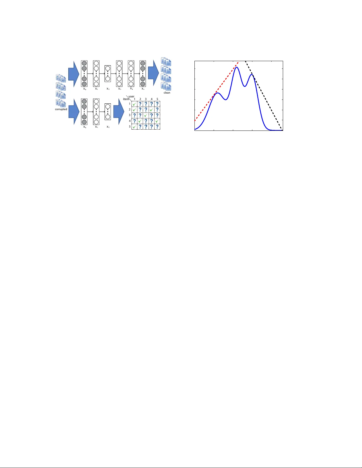
A Survey on Bayesian Deep Learning HA O W ANG, Massachusetts Institute of T echnology, USA DI T - Y AN YEUNG, Hong Kong University of Science and T echnology, Hong Kong A comprehensive articial intelligence system needs to not only perceive the envir onment with dierent ‘senses’ ( e.g., seeing and hearing) but also infer the w orld’s conditional (or e ven causal) relations and corr esponding uncertainty . The past decade has seen major advances in many perception tasks such as visual object recognition and speech recognition using deep learning mo dels. For higher-level inference, howe ver , probabilistic graphical models with their Bayesian nature are still more p owerful and exible. In recent years, Bayesian de ep learning has emerged as a unied probabilistic framework to tightly integrate deep learning and Bayesian models 1 . In this general framework, the perception of text or images using deep learning can boost the performance of higher-level inference and in turn, the feedback from the infer ence process is able to enhance the perception of te xt or images. This survey provides a comprehensive introduction to Bay esian deep learning and reviews its recent applications on recommender systems, topic models, control, etc. Besides, we also discuss the relationship and dierences between Bayesian deep learning and other related topics such as Bayesian treatment of neural networks. CCS Concepts: • Mathematics of computing → Probabilistic r epresentations ; • Information systems → Data mining ; • Computing methodologies → Neural networks . Additional K ey W ords and Phrases: Deep Learning, Bayesian Networks, Probabilistic Graphical Models, Generative Models A CM Reference Format: Hao W ang and Dit- Y an Y eung. 2020. A Survey on Bayesian Deep Learning. In A CM Computing Sur veys. ACM, New Y ork, NY, USA, Article 1, 35 pages. https://doi.org/10.1145/3409383 1 INTRODUCTION Over the past decade, de ep learning has achieved signicant success in many popular perception tasks including visual object recognition, text understanding, and speech recognition. These tasks correspond to articial intelligence (AI) systems’ ability to see , read , and hear , respe ctively , and they are undoubtedly indispensable for AI to eectively perceiv e the environment. Howev er , in order to build a practical and comprehensive AI system, simply being able to perceive is far from sucient. It should, above all, possess the ability of thinking . A typical example is me dical diagnosis, which goes far bey ond simple perception: besides se eing visible symptoms (or medical images from CT) and hearing descriptions from patients, a doctor also has to look for relations among all the symptoms and preferably infer their corresponding etiology . Only after that can the do ctor provide medical advice for the patients. In this example, although the abilities of seeing and hearing allow the do ctor to acquire information from the patients, it is the thinking part that denes a doctor . Specically , the ability of thinking here could inv olve identifying conditional dependencies, causal inference, logic deduction, and dealing with uncertainty , which are appar ently beyond 1 See a curated and updating list of papers related to Bayesian deep learning at https://github.com/js05212/BayesianDeepLearning- Survey . Permission to make digital or hard copies of all or part of this w ork for personal or classroom use is granted without fee provided that copies are not made or distributed for prot or commercial advantage and that copies bear this notice and the full citation on the rst page. Copyrights for components of this work owned by others than the author(s) must be honored. Abstracting with credit is permitted. T o copy otherwise, or republish, to post on servers or to redistribute to lists, requires prior specic permission and /or a fe e. Request permissions from permissions@acm.org. © 2020 Copyright held by the owner/author(s). Publication rights licensed to A CM. Manuscript submitted to ACM 1 CSUR, March, 2020, New Y ork, NY Hao W ang and Dit-Y an Y eung the capability of conventional deep learning methods. Fortunately , another machine learning paradigm, probabilistic graphical models (PGM), excels at probabilistic or causal inference and at dealing with uncertainty . The problem is that PGM is not as good as deep learning mo dels at perception tasks, which usually involve large-scale and high-dimensional signals (e .g., images and videos). T o address this problem, it is therefore a natural choice to unify deep learning and PGM within a principled probabilistic framework, which we call Bay esian deep learning (BDL) in this pap er . In the example abov e, the perception task involves perceiving the patient’s symptoms (e.g., by seeing me dical images), while the inference task inv olves handling conditional dependencies, causal inference, logic deduction, and uncertainty . With the principled integration in Bayesian deep learning, the perception task and inference task are regarded as a whole and can benet from each other . Concretely , being able to see the medical image could help with the doctor’s diagnosis and inference. On the other hand, diagnosis and inference can, in turn, help understand the medical image . Suppose the doctor may not be sure ab out what a dark spot in a medical image is, but if she is able to infer the etiology of the symptoms and disease, it can help her better decide whether the dark spot is a tumor or not. T ake recommender systems [ 1 , 70 , 71 , 92 , 121 ] as another example. A highly accurate recommender system requires (1) thorough understanding of item content ( e.g., content in documents and movies) [ 85 ], (2) careful analysis of users’ proles/preferences [ 126 , 130 , 134 ], and (3) proper evaluation of similarity among users [ 3 , 12 , 46 , 109 ]. Deep learning with its ability to eciently process dense high-dimensional data such as movie content is good at the rst subtask, while PGM specializing in mo deling conditional dep endencies among users, items, and ratings (see Figure 7 as an example, where u , v , and R are user latent vectors, item latent vectors, and ratings, respectively) e xcels at the other two. Hence unifying them two in a single principled probabilistic framework gets us the b est of both worlds. Such integration also comes with additional benet that uncertainty in the recommendation process is handled elegantly . What’s more, one can also deriv e Bayesian treatments for concrete models, leading to mor e robust predictions [ 68 , 121 ]. As a third example, consider contr olling a complex dynamical system according to the live video stream r eceived from a camera. This problem can be transformed into iterativ ely performing two tasks, p erception from raw images and control based on dynamic models. The perception task of pr ocessing raw images can be handled by deep learning while the control task usually needs more sophisticated models such as hidden Marko v models and Kalman lters [ 35 , 74 ]. The feedback loop is then completed by the fact that actions chosen by the control model can aect the received video stream in turn. T o enable an ee ctive iterative process between the perception task and the control task, we nee d information to ow back and forth between them. The p erception component would be the basis on which the control component estimates its states and the control comp onent with a dynamic model built in would be able to predict the future trajectory (images). Therefore Bayesian deep learning is a suitable choice [ 125 ] for this problem. Note that similar to the recommender system example, both noise from raw images and uncertainty in the control process can be naturally dealt with under such a probabilistic framework. The above examples demonstrate BDL’s major advantages as a principled way of unifying deep learning and PGM: information exchange between the perception task and the inference task , conditional dependencies on high-dimensional data, and ee ctive modeling of uncertainty . In terms of uncertainty , it is worth noting that when BDL is applied to complex tasks, there are thr ee kinds of parameter uncertainty that need to be taken into account: (1) Uncertainty on the neural network parameters. (2) Uncertainty on the task-specic parameters. (3) Uncertainty of exchanging information between the perception component and the task-specic comp onent. By representing the unknown parameters using distributions instead of p oint estimates, BDL oers a promising framework to handle these three kinds of uncertainty in a unied way . It is worth noting that the third uncertainty 2 A Survey on Bayesian Deep Learning CSUR, March, 2020, New Y ork, NY could only be handled under a unied framework like BDL; training the perception component and the task-specic component separately is equivalent to assuming no uncertainty when exchanging information between them two. Note that neural networks are usually over-parameterized and therefor e pose additional challenges in eciently handling the uncertainty in such a large parameter space. On the other hand, graphical models are often more concise and have smaller parameter space, providing better interpretability . Besides the advantages above, another benet comes from the implicit regularization built in BDL. By imposing a prior on hidden units, parameters dening a neural network, or the model parameters specifying the conditional dependencies, BDL can to some degree avoid overtting, especially when we have insucient data. Usually , a BDL model consists of two components, a perception component that is a Bay esian formulation of a certain type of neural networks and a task-specic component that describes the relationship among dier ent hidden or observed variables using PGM. Regularization is crucial for them both. Neural networks are usually heavily over-parameterized and therefore ne eds to be regularized properly . Regularization te chniques such as weight decay and dropout [ 103 ] are shown to be eective in improving performance of neural networks and they both have Bayesian interpretations [ 22 ]. In terms of the task-sp ecic component, expert knowledge or prior information, as a kind of regularization, can be incorporated into the model through the prior we imposed to guide the model when data are scarce. There are also challenges when applying BDL to real-world tasks. (1) First, it is nontrivial to design an ecient Bayesian formulation of neural networks with reasonable time complexity . This line of work is pioneered by [ 42 , 72 , 80 ], but it has not been widely adopted due to its lack of scalability . Fortunately , some recent advances in this direction [ 2 , 9 , 31 , 39 , 58 , 119 , 121 ] seem to shed light 2 on the practical adoption of Bayesian neural network 3 . (2) The second challenge is to ensure ecient and ee ctive information exchange b etween the perception component and the task-specic component. Ideally both the rst-order and second-order information (e.g., the mean and the variance) should be able to ow back and forth between the two components. A natural way is to repr esent the perception component as a PGM and seamlessly connect it to the task-specic PGM, as done in [ 24 , 118 , 121 ]. This survey provides a comprehensiv e overview of BDL with concrete models for various applications. The rest of the survey is organized as follows: In Section 2 , we provide a review of some basic deep learning models. Section 3 covers the main concepts and techniques for PGM. These two se ctions serve as the preliminaries for BDL, and the next section, Section 4 , demonstrates the rationale for the unied BDL framework and details various choices for implementing its p erception component and task-specic comp onent . Section 5 reviews the BDL mo dels applied to various areas such as r ecommender systems, topic models, and control, show casing how BDL works in supervised learning, unsupervise d learning, and general representation learning, respectively . Section 6 discusses some future research issues and concludes the paper . 2 DEEP LEARNING Deep learning normally refers to neural networks with more than two layers. T o better understand deep learning, here we start with the simplest type of neural networks, multilay er perceptrons (MLP), as an e xample to show how conventional deep learning w orks. After that, we will review sev eral other types of deep learning models based on MLP . 2 In summary , reduction in time complexity can be achieved via e xpectation propagation [ 39 ], the reparameterization trick [ 9 , 58 ], probabilistic formulation of neural networks with maximum a posteriori estimates [ 121 ], approximate variational inference with natural-parameter netw orks [ 119 ], knowledge distillation [ 2 ], etc. W e refer readers to [ 119 ] for a detailed overview . 3 Here we refer to the Bayesian treatment of neural networks as Bayesian neural networks. The other term, Bayesian deep learning, is retained to refer to complex Bayesian models with both a perception component and a task-specic component. Se e Section 4.1 for a detailed discussion. 3 CSUR, March, 2020, New Y ork, NY Hao W ang and Dit-Y an Y eung X 0 X 0 X 1 X 1 X 2 X 2 X 3 X 3 X 4 X 4 X c X c Fig. 1. Le: A 2-layer SD AE with 𝐿 = 4 . Right: A convolutional layer with 4 input feature maps and 2 output feature maps. 2.1 Multilayer Perceptrons Essentially a multilayer perceptron is a sequence of parametric nonlinear transformations. Suppose we want to train a multilayer perceptron to perform a regression task which maps a vector of 𝑀 dimensions to a vector of 𝐷 dimensions. W e denote the input as a matrix X 0 ( 0 means it is the 0 -th layer of the perceptron). The 𝑗 -th row of X 0 , denoted as X 0 , 𝑗 ∗ , is an 𝑀 -dimensional vector representing one data point. The target (the output w e want to t) is denoted as Y . Similarly Y 𝑗 ∗ denotes a 𝐷 -dimensional row v ector . The problem of learning an 𝐿 -layer multilayer perceptr on can be formulated as the following optimization problem: min { W 𝑙 } , { b 𝑙 } ∥ X 𝐿 − Y ∥ 𝐹 + 𝜆 𝑙 ∥ W 𝑙 ∥ 2 𝐹 subject to X 𝑙 = 𝜎 ( X 𝑙 − 1 W 𝑙 + b 𝑙 ) , 𝑙 = 1 , . . . , 𝐿 − 1 X 𝐿 = X 𝐿 − 1 W 𝐿 + b 𝐿 , where 𝜎 ( ·) is an element-wise sigmoid function for a matrix and 𝜎 ( 𝑥 ) = 1 1 + exp ( − 𝑥 ) . ∥ · ∥ 𝐹 denotes the Frobenius norm. The purpose of imposing 𝜎 ( ·) is to allow nonlinear transformation. Normally other transformations like tanh ( 𝑥 ) and max ( 0 , 𝑥 ) can be used as alternatives of the sigmoid function. Here X 𝑙 ( 𝑙 = 1 , 2 , . . . , 𝐿 − 1 ) is the hidden units. As we can see, X 𝐿 can be easily computed once X 0 , W 𝑙 , and b 𝑙 are given. Since X 0 is given as input, one only needs to learn W 𝑙 and b 𝑙 here. Usually this is done using backpropagation and stochastic gradient descent (SGD). The key is to compute the gradients of the objective function with respect to W 𝑙 and b 𝑙 . Denoting the value of the objective function as 𝐸 , one can compute the gradients using the chain rule as: 𝜕𝐸 𝜕 X 𝐿 = 2 ( X 𝐿 − Y ) , 𝜕𝐸 𝜕 X 𝑙 = ( 𝜕𝐸 𝜕 X 𝑙 + 1 ◦ X 𝑙 + 1 ◦ ( 1 − X 𝑙 + 1 ) ) W 𝑙 + 1 , 𝜕𝐸 𝜕 W 𝑙 = X 𝑇 𝑙 − 1 ( 𝜕𝐸 𝜕 X 𝑙 ◦ X 𝑙 ◦ ( 1 − X 𝑙 ) ) , 𝜕𝐸 𝜕 b 𝑙 = 𝑚𝑒 𝑎𝑛 ( 𝜕𝐸 𝜕 X 𝑙 ◦ X 𝑙 ◦ ( 1 − X 𝑙 ) , 1 ) , where 𝑙 = 1 , . . . , 𝐿 and the regularization terms are omitted. ◦ denotes the element-wise product and 𝑚𝑒 𝑎𝑛 ( · , 1 ) is the matlab operation on matrices. In practice, w e only use a small part of the data (e .g., 128 data points) to compute the gradients for each update. This is called stochastic gradient descent. As we can see, in conventional deep learning models, only W 𝑙 and b 𝑙 are free parameters, which we will update in each iteration of the optimization. X 𝑙 is not a free parameter since it can be computed exactly if W 𝑙 and b 𝑙 are given. 4 A Survey on Bayesian Deep Learning CSUR, March, 2020, New Y ork, NY 2.2 A utoencoders An autoencoder (AE) is a fee dforward neural network to encode the input into a more compact representation and reconstruct the input with the learned representation. In its simplest form, an autoencoder is no more than a multilay er perceptron with a bottleneck lay er (a layer with a small number of hidden units) in the middle. The idea of autoencoders has been around for decades [ 10 , 29 , 43 , 63 ] and abundant variants of autoencoders have been proposed to enhance representation learning including sparse AE [ 88 ], contrastive AE [ 93 ], and denoising AE [ 111 ]. For more details, please refer to a nice recent book on deep learning [ 29 ]. Here we introduce a kind of multilayer denoising AE, known as stacked denoising autoencoders (SDAE), both as an example of AE variants and as background for its applications on BDL-based recommender systems in Section 4 . SD AE [ 111 ] is a fee dforward neural network for learning representations (encoding) of the input data by learning to predict the clean input itself in the output, as shown in Figure 1 ( left). The hidden layer in the middle, i.e., X 2 in the gure, can be constrained to be a bottleneck to learn compact representations. The dierence between traditional AE and SD AE is that the input layer X 0 is a corrupted version of the clean input data X 𝑐 . Essentially an SD AE solves the following optimization problem: min { W 𝑙 } , { b 𝑙 } ∥ X 𝑐 − X 𝐿 ∥ 2 𝐹 + 𝜆 𝑙 ∥ W 𝑙 ∥ 2 𝐹 subject to X 𝑙 = 𝜎 ( X 𝑙 − 1 W 𝑙 + b 𝑙 ) , 𝑙 = 1 , . . . , 𝐿 − 1 X 𝐿 = X 𝐿 − 1 W 𝐿 + b 𝐿 , where 𝜆 is a regularization parameter . Here SDAE can be regarded as a multilayer perceptron for regression tasks described in the previous section. The input X 0 of the MLP is the corrupted version of the data and the target Y is the clean version of the data X 𝑐 . For example , X 𝑐 can be the raw data matrix, and we can randomly set 30% of the entries in X 𝑐 to 0 and get X 0 . In a nutshell, SDAE learns a neural network that takes the noisy data as input and recovers the clean data in the last layer . This is what ‘ denoising’ in the name means. Normally , the output of the middle layer , i.e., X 2 in Figure 1 (left), would be used to compactly represent the data. 2.3 Convolutional Neural Networks Convolutional neural networks (CNN) can be view ed as another variant of MLP. Dierent from AE, which is initially designed to perform dimensionality reduction, CNN is biologically inspired. According to [ 53 ], two types of cells have been identied in the cat’s visual cortex. One is simple cells that respond maximally to specic patterns within their receptive eld, and the other is complex cells with larger receptive eld that are considered locally invariant to positions of patterns. Inspired by these ndings, the two key concepts in CNN are then developed: convolution and max-pooling. Convolution : In CNN, a feature map is the result of the convolution of the input and a linear lter , follow ed by some element-wise nonlinear transformation. The input here can be the raw image or the feature map from the pre vious layer . Specically , with input X , weights W 𝑘 , bias 𝑏 𝑘 , the 𝑘 -th feature map H 𝑘 can be obtained as follows: H 𝑘 𝑖 𝑗 = tanh ( ( W 𝑘 ∗ X ) 𝑖 𝑗 + 𝑏 𝑘 ) . Note that in the equation ab ove w e assume one single input feature map and multiple output feature maps. In practice, CNN often has multiple input feature maps as well due to its deep structure. A convolutional layer with 4 input feature maps and 2 output feature maps is shown in Figure 1 (right). 5 CSUR, March, 2020, New Y ork, NY Hao W ang and Dit-Y an Y eung x x W W z z V V o o x t x t h t h t o t o t W W x 1 x 1 h 1 h 1 o 1 o 1 Y Y V V x 2 x 2 h 2 h 2 o 2 o 2 Y Y V V . . . . . . x T x T h T h T o T o T Y Y V V W W W W Fig. 2. Le: A conventional feedforward neural network with one hidden layer , where x is the input, z is the hidden layer , and o is the output, W and V are the corresponding weights (biases are omied her e). Middle: A recurrent neural network with input { x 𝑡 } 𝑇 𝑡 = 1 , hidden states { h 𝑡 } 𝑇 𝑡 = 1 , and output { o 𝑡 } 𝑇 𝑡 = 1 . Right: An unrolled RNN which is equivalent to the one in Figur e 2 (middle). Here each node (e.g., x 1 , h 1 , or o 1 ) is associated with one particular time step. Max-Pooling : Traditionally , a convolutional layer in CNN is followed by a max-p ooling layer , which can be seen as a type of nonlinear downsampling. The operation of max-pooling is simple. For example, if we have a feature map of size 6 × 9 , the result of max-pooling with a 3 × 3 region would be a downsampled feature map of size 2 × 3 . Each entry of the downsampled feature map is the maximum value of the corresponding 3 × 3 region in the 6 × 9 feature map. Max-pooling layers can not only reduce computational cost by ignoring the non-maximal entries but also provide local translation invariance. Putting it all together : Usually to form a complete and working CNN, the input would alternate b etween convolutional layers and max-pooling layers before going into an MLP for tasks such as classication or regr ession. One classic example is the LeNet-5 [ 64 ], which alternates between 2 convolutional layers and 2 max-pooling layers before going into a fully connected MLP for target tasks. 2.4 Recurrent Neural Network When reading an article , one normally takes in one word at a time and tr y to understand the curr ent word based on previous wor ds. This is a recurrent process that needs short-term memory . Unfortunately conventional feedforward neural networks like the one shown in Figure 2 (left) fail to do so. For example, imagine w e want to constantly predict the next word as we read an article . Since the fee dforward network only computes the output o as V 𝑞 ( Wx ) , where the function 𝑞 ( ·) denotes element-wise nonlinear transformation, it is unclear how the network could naturally model the sequence of words to predict the next wor d. 2.4.1 V anilla Recurrent Neural Network. T o solve the problem, we need a recurrent neural netw ork [ 29 ] instead of a feedfor ward one. A s shown in Figure 2 (middle), the computation of the current hidden states h 𝑡 depends on the current input x 𝑡 (e.g., the 𝑡 -th word) and the previous hidden states h 𝑡 − 1 . This is why there is a loop in the RNN. It is this loop that enables short-term memory in RNNs. The h 𝑡 in the RNN represents what the netw ork knows so far at the 𝑡 -th time step. T o see the computation more clearly , we can unroll the loop and represent the RNN as in Figure 2 (right). If we use hyperbolic tangent nonlinearity ( tanh ), the computation of output o 𝑡 will be as follows: a 𝑡 = Wh 𝑡 − 1 + Yx 𝑡 + b , h 𝑡 = tanh ( a 𝑡 ) , o 𝑡 = Vh 𝑡 + c , where Y , W , and V denote the weight matrices for input-to-hidden, hidden-to-hidden, and hidden-to-output connections, respectively , and b and c are the corresponding biases. If the task is to classify the input data at each time step, we can 6 A Survey on Bayesian Deep Learning CSUR, March, 2020, New Y ork, NY A B C $ A B C $ Fig. 3. The encoder-deco der architecture involving two LSTMs. The encoder LSTM (in the le rectangle) encodes the se quence ‘ ABC’ into a representation and the decoder LSTM (in the right rectangle) recovers the sequence from the representation. ‘$’ marks the end of a sentence. compute the classication probability as p 𝑡 = softmax ( o 𝑡 ) where softmax ( q ) = exp ( q ) Í 𝑖 exp ( q 𝑖 ) . Similar to feedforward networks, an RNN is traine d with a generalized back-propagation algorithm called back-propagation through time (BPT T) [ 29 ]. Essentially the gradients are computed through the unrolled netw ork as shown in Figure 2 (right) with shared weights and biases for all time steps. 2.4.2 Gated Re current Neural Network. The problem with the vanilla RNN ab ove is that the gradients propagated over many time steps are prone to vanish or explode, making the optimization notoriously dicult. In addition, the signal passing through the RNN decays exponentially , making it imp ossible to model long-term dependencies in long sequences. Imagine we want to predict the last w ord in the paragraph ‘I have many books ... I like reading ’ . In order to get the answer , we need ‘long-term memory’ to retrieve information (the w ord ‘books’) at the start of the text. T o address this problem, the long short-term memory mo del (LSTM) is designed as a type of gated RNN to model and accumulate information over a relatively long duration. The intuition behind LSTM is that when processing a sequence consisting of several subsequences, it is sometimes useful for the neural network to summarize or forget the old states before moving on to process the next subsequence [ 29 ]. Using 𝑡 = 1 . . . 𝑇 𝑗 to index the words in the sequence, the formulation of LSTM is as follows (w e drop the item index 𝑗 for notational simplicity): x 𝑡 = W 𝑤 e 𝑡 , s 𝑡 = h 𝑓 𝑡 − 1 ⊙ s 𝑡 − 1 + h 𝑖 𝑡 − 1 ⊙ 𝜎 ( Yx 𝑡 − 1 + Wh 𝑡 − 1 + b ) , (1) where x 𝑡 is the word embedding of the 𝑡 -th word, W 𝑤 is a 𝐾 𝑊 -by- 𝑆 word emb edding matrix, and e 𝑡 is the 1 -of- 𝑆 representation, ⊙ stands for the element-wise product operation between two vectors, 𝜎 ( · ) denotes the sigmoid function, s 𝑡 is the cell state of the 𝑡 -th word, and b , Y , and W denote the biases, input weights, and recurrent weights respectively . The forget gate units h 𝑓 𝑡 and the input gate units h 𝑖 𝑡 in Equation ( 1 ) can be computed using their corresponding weights and biases Y 𝑓 , W 𝑓 , Y 𝑖 , W 𝑖 , b 𝑓 , and b 𝑖 : h 𝑓 𝑡 = 𝜎 ( Y 𝑓 x 𝑡 + W 𝑓 h 𝑡 + b 𝑓 ) , h 𝑖 𝑡 = 𝜎 ( Y 𝑖 x 𝑡 + W 𝑖 h 𝑡 + b 𝑖 ) . The output depends on the output gate h 𝑜 𝑡 which has its own weights and biases Y 𝑜 , W 𝑜 , and b 𝑜 : h 𝑡 = tanh ( s 𝑡 ) ⊙ h 𝑜 𝑡 − 1 , h 𝑜 𝑡 = 𝜎 ( Y 𝑜 x 𝑡 + W 𝑜 h 𝑡 + b 𝑜 ) . Note that in the LSTM, information of the processed sequence is contained in the cell states s 𝑡 and the output states h 𝑡 , both of which are column vectors of length 𝐾 𝑊 . Similar to [ 16 , 108 ], we can use the output state and cell state at the last time step ( h 𝑇 𝑗 and s 𝑇 𝑗 ) of the rst LSTM as the initial output state and cell state of the second LSTM. This way the two LSTMs can b e concatenated to form an encoder-decoder architecture, as shown in Figure 3 . 7 CSUR, March, 2020, New Y ork, NY Hao W ang and Dit-Y an Y eung k K J z w D Fig. 4. The probabilistic graphical model for LDA, 𝐽 is the number of documents, 𝐷 is the number of words in a document, and 𝐾 is the number of topics. Note that there is a vast literature on deep learning and neural networks. The introduction in this se ction intends to serve only as the background of Bayesian deep learning. Readers are referred to [ 29 ] for a comprehensive survey and more details. 3 PROBABILISTIC GRAPHICAL MODELS Probabilistic Graphical Models (PGM) use diagrammatic representations to describe random variables and relationships among them. Similar to a graph that contains nodes (vertices) and links ( edges), PGM has nodes to represent random variables and links to indicate probabilistic relationships among them. 3.1 Models There are essentially tw o types of PGM, directed PGM (also known as Bayesian networks) and undir ected PGM (also known as Markov random elds) [ 5 ]. In this survey we mainly focus on directed PGM 4 . For details on undirected PGM, readers are referr ed to [ 5 ]. A classic example of PGM would be latent Dirichlet allocation (LDA), which is used as a topic model to analyze the generation of words and topics in documents [ 8 ]. Usually PGM comes with a graphical representation of the model and a generative process to depict the story of how the random variables are generated step by step . Figure 4 shows the graphical model for LDA and the corr esponding generative process is as follows: • For each document 𝑗 ( 𝑗 = 1 , 2 , . . . , 𝐽 ), (1) Draw topic proportions 𝜃 𝑗 ∼ Dirichlet ( 𝛼 ) . (2) For each word 𝑤 𝑗 𝑛 of item (document) w 𝑗 , (a) Draw topic assignment 𝑧 𝑗 𝑛 ∼ Mult ( 𝜃 𝑗 ) . (b) Draw word 𝑤 𝑗 𝑛 ∼ Mult ( 𝛽 𝑧 𝑗 𝑛 ) . The generative process above provides the story of how the random variables are generated. In the graphical model in Figure 4 , the shaded no de denotes observed variables while the others are latent variables ( 𝜽 and z ) or parameters ( 𝛼 and 𝛽 ). Once the model is dened, learning algorithms can be applied to automatically learn the latent variables and parameters. Due to its Bayesian nature, PGM such as LDA is easy to extend to incorporate other information or to perform other tasks. For example, following LDA, dierent variants of topic models have been proposed. [ 7 , 113 ] are proposed to incorporate temporal information, and [ 6 ] extends LDA by assuming correlations among topics. [ 44 ] extends LDA from the batch mo de to the online setting, making it possible to process large datasets. On recommender systems, collaborative topic regression (CTR) [ 112 ] extends LD A to incorporate rating information and make recommendations. This model is then further extended to incorporate social information [ 89 , 115 , 116 ]. 4 For convenience, PGM stands for directed PGM in this survey unless specied otherwise. 8 A Survey on Bayesian Deep Learning CSUR, March, 2020, New Y ork, NY T able 1. Summary of BDL Models with Dierent Learning Algorithms (MAP: Maximum a Posteriori, VI: V ariational Inference, Hybrid MC: Hybrid Monte Carlo) and Dierent V ariance T ypes (ZV: Zero- V ariance, H V: Hyper- Variance , LV: Learnable- V ariance). Applications Models V ariance of 𝛀 ℎ MAP VI Gibbs Sampling Hybrid MC Recommender Systems Collaborative Deep Learning (CDL) [ 121 ] HV ✓ Bayesian CDL [ 121 ] HV ✓ Marginalized CDL [ 66 ] LV ✓ Symmetric CDL [ 66 ] LV ✓ Collaborative Deep Ranking [ 131 ] HV ✓ Collaborative Knowledge Base Embedding [ 132 ] H V ✓ Collaborative Recurrent AE [ 122 ] HV ✓ Collaborative V ariational Autoencoders [ 68 ] HV ✓ T opic Models Relational SDAE HV ✓ Deep Poisson Factor Analysis with Sigmoid Belief Networks [ 24 ] ZV ✓ ✓ Deep Poisson Factor Analysis with Restricted Boltzmann Machine [ 24 ] ZV ✓ ✓ Deep Latent Dirichlet Allocation [ 18 ] LV ✓ Dirichlet Belief Networks [ 133 ] LV ✓ Control Embed to Control [ 125 ] LV ✓ Deep V ariational Bayes Filters [ 57 ] LV ✓ Probabilistic Recurrent State-Space Models [ 19 ] LV ✓ Deep Planning Networks [ 34 ] LV ✓ Link Prediction Relational Deep Learning [ 120 ] LV ✓ ✓ Graphite [ 32 ] LV ✓ Deep Generative Latent Feature Relational Model [ 75 ] LV ✓ NLP Sequence to Better Sequence [ 77 ] LV ✓ Quantiable Sequence Editing [ 69 ] LV ✓ Computer Vision Asynchronous T emporal Fields [ 102 ] LV ✓ Attend, Infer , Repeat (AIR) [ 20 ] LV ✓ Fast AIR [ 105 ] LV ✓ Sequential AIR [ 60 ] LV ✓ Speech Factorized Hierarchical V AE [ 48 ] LV ✓ Scalable Factorized Hierarchical V AE [ 47 ] LV ✓ Gaussian Mixture V ariational Autoencoders [ 49 ] LV ✓ Recurrent Poisson Process Units [ 51 ] LV ✓ ✓ Deep Graph Random Process [ 52 ] LV ✓ ✓ Time Series Forecasting DeepAR [ 21 ] LV ✓ DeepState [ 90 ] LV ✓ Spline Quantile Function RNN [ 27 ] LV ✓ DeepFactor [ 124 ] LV ✓ Health Care Deep Poisson Factor Models [ 38 ] LV ✓ Deep Markov Models [ 61 ] LV ✓ Black-Box False Discovery Rate [ 110 ] LV ✓ Bidirectional Inference Networks [ 117 ] LV ✓ 3.2 Inference and Learning Strictly speaking, the process of nding the parameters (e.g., 𝛼 and 𝛽 in Figure 4 ) is called learning and the process of nding the latent variables (e.g., 𝜽 and z in Figure 4 ) given the parameters is called inference. Howev er , given only the observed variables (e.g. w in Figure 4 ), learning and inference are often intertwined. Usually the learning and inference of LDA w ould alternate between the updates of latent variables (which correspond to inference) and the updates of the parameters (which correspond to learning). Once the learning and inference of LDA is completed, one could obtain the learned parameters 𝛼 and 𝛽 . If a new document comes, one can now x the learne d 𝛼 and 𝛽 and then perform inference alone to nd the topic proportions 𝜃 𝑗 of the new document. 5 Similar to LD A, various learning and inference algorithms are available for each PGM. Among them, the most cost-eective one is probably maximum a posteriori (MAP), which amounts to maximizing the p osterior probability of the latent variable. Using MAP, the learning process is equivalent to minimizing (or maximizing) an objective function with regularization. One famous example is the probabilistic matrix factorization (PMF) [ 96 ], where the learning of the graphical model is equivalent to factorizing a large matrix into two low-rank matrices with L2 regularization. MAP, as ecient as it is, gives us only point estimates of latent variables (and parameters). In order to take the uncertainty into account and harness the full power of Bayesian models, one would have to resort to Bayesian treatments such as variational inference and Markov chain Monte Carlo (MCMC). For example, the original LD A uses variational 5 For convenience, we use ‘learning’ to repr esent both ‘learning and inference’ in the following text. 9 CSUR, March, 2020, New Y ork, NY Hao W ang and Dit-Y an Y eung inference to appro ximate the true posterior with factorized variational distributions [ 8 ]. Learning of the latent variables and parameters then boils down to minimizing the KL-divergence between the variational distributions and the true posterior distributions. Besides variational inference, another choice for a Bayesian treatment is MCMC. For example , MCMC algorithms such as [ 86 ] have been proposed to learn the posterior distributions of LDA. 4 BA YESIAN DEEP LEARNING With the preliminaries on deep learning and PGM, w e are now ready to intr oduce the general framework and some concrete e xamples of BDL. Sp ecically , in this section we will list some recent BDL models with applications on recommender systems, topic models, control, etc. A summary of these models is shown in T able 1 . 4.1 A Brief History of Bayesian Neural Networks and Bayesian Deep Learning One topic highly related to BDL is Bayesian neural networks (BNN) or Bayesian treatments of neural networks. Similar to any Bayesian treatment, BNN imp oses a prior on the neural network’s parameters and aims to learn a posterior distribution of these parameters. During the inference phrase, such a distribution is then marginalized out to produce nal pr edictions. In general such a process is called Bayesian model av eraging [ 5 ] and can be seen as learning an innite number of (or a distribution over ) neural networks and then aggregating the results thr ough ensembling. The study of BNN dates back to 1990s with notable works from [ 42 , 72 , 80 ]. O ver the years, a large b ody of works [ 2 , 9 , 31 , 39 , 58 , 100 ] have emerged to enable substantially b etter scalability and incorp orate recent advancements of deep neural networks. Due to BNN’s long history , the term ‘Bayesian deep learning’ sometimes specically refers to ‘Bayesian neural networks’ [ 73 , 128 ]. In this survey , we instead use ‘Bayesian deep learning’ in a broader sense to refer to the probabilistic frame work subsuming Bayesian neural networks. T o see this, note that a BDL model with a perception comp onent and an empty task-specic component is equivalent to a Bayesian neural network ( details on these two components are discussed in Section 4.2 ). Interestingly , though BNN started in 1990s, the study of BDL in a broader sense started roughly in 2014 [ 38 , 114 , 118 , 121 ], slightly after the deep learning breakthrough in the ImageNet LSVRC contest in 2012 [ 62 ]. As we will see in later sections, BNN is usually used as a perception component in BDL models. T oday BDL is gaining more and more popularity , has found successful applications in ar eas such as recommender systems and computer vision, and appears as the theme of various conference workshops (e .g., the NeurIPS BDL workshop 6 ). 4.2 General Framework As mentioned in Section 1 , BDL is a principle d probabilistic framew ork with two seamlessly integrated components: a perception comp onent and a task-specic comp onent . T wo Comp onents : Figure 5 shows the PGM of a simple BDL model as an example. The part inside the red rectangle on the left represents the perception component and the part inside the blue rectangle on the right is the task-specic component. T ypically , the perception component would be a probabilistic formulation of a deep learning model with multiple nonlinear processing layers represented as a chain structure in the PGM. While the no des and edges in the perception component are relatively simple, those in the task-specic component often describe more complex distributions and relationships among variables. Concretely , a task-sp ecic component can take various forms. For 6 http://bayesiandeeplearning.org/ 10 A Survey on Bayesian Deep Learning CSUR, March, 2020, New Y ork, NY 𝑿 𝟎 𝑿 𝟏 𝑿 𝟐 𝑿 𝟑 𝑿 𝟒 𝑾 𝟏 𝑾 𝟐 𝑾 𝟑 𝑾 𝟒 H A B C D Fig. 5. The PGM for an e xample BDL. The red r ectangle on the le indicates the per ception component, and the blue rectangle on the right indicates the task-specific component. The hinge variable 𝛀 ℎ = { H } . example, it can be a typical Bayesian network (directed PGM) such as LD A, a deep Bayesian network [ 117 ], or a stochastic process [ 51 , 94 ], all of which can be represented in the form of PGM. Three V ariable Sets : There are thr ee sets of variables in a BDL model: perception variables, hinge variables, and task variables. In this paper , we use 𝛀 𝑝 to denote the set of perception variables (e .g., X 0 , X 1 , and W 1 in Figure 5 ), which are the variables in the perception component. Usually 𝛀 𝑝 would include the weights and neurons in the probabilistic formulation of a deep learning mo del. 𝛀 ℎ is used to denote the set of hinge variables (e .g. H in Figur e 5 ). These variables directly interact with the perception component from the task-specic comp onent. The set of task variables (e .g. A , B , and C in Figure 5 ), i.e., variables in the task-spe cic component without direct relation to the perception component, is denoted as 𝛀 𝑡 . Generative Processes for Super vised and Unsupervise d Learning : If the edges between the two components point towards 𝛀 ℎ , the joint distribution of all variables can be written as: 𝑝 ( 𝛀 𝑝 , 𝛀 ℎ , 𝛀 𝑡 ) = 𝑝 ( 𝛀 𝑝 ) 𝑝 ( 𝛀 ℎ | 𝛀 𝑝 ) 𝑝 ( 𝛀 𝑡 | 𝛀 ℎ ) . (2) If the edges between the two components originate from 𝛀 ℎ , the joint distribution of all variables can be written as: 𝑝 ( 𝛀 𝑝 , 𝛀 ℎ , 𝛀 𝑡 ) = 𝑝 ( 𝛀 𝑡 ) 𝑝 ( 𝛀 ℎ | 𝛀 𝑡 ) 𝑝 ( 𝛀 𝑝 | 𝛀 ℎ ) . (3) Equation ( 2 ) and ( 3 ) assume dierent generative processes for the data and corr espond to dierent learning tasks. The former is usually used for sup ervised learning, where the perception comp onent serves as a probabilistic (or Bayesian) representation learner to facilitate any downstream tasks (see Section 5.1 for some examples). The latter is usually used for unsupervise d learning, where the task-specic component provides structured constraints and domain knowledge to help the perception component learn stronger representations ( see Section 5.2 for some examples). Note that b esides these two vanilla cases, it is possible for BDL to simultaneously have some edges between the two components pointing towards 𝛀 ℎ and some originating from 𝛀 ℎ , in which case the decomposition of the joint distribution would be more complex. Independence Re quirement : The introduction of hinge variables 𝛀 ℎ and related conditional distributions simplies the model (especially when 𝛀 ℎ ’s in-degree or out-degree is 1 ), facilitate learning, and provides inductive bias to concentrate information inside 𝛀 ℎ . Note that hinge variables are always in the task-specic component; the connections between hinge variables 𝛀 ℎ and the perception component (e.g., X 4 → H in Figure 5 ) should normally b e independent for convenience of parallel computation in the perception component. For example, each ro w in H is related to only one corresponding row in X 4 . Although it is not mandatory in BDL models, meeting this requirement would signicantly increase the eciency of parallel computation in model training. Flexibility of V ariance for 𝛀 ℎ : As mentioned in Section 1 , one of BDL’s motivations is to model the uncertainty of exchanging information b etween the perception component and the task-specic component, which boils down to 11 CSUR, March, 2020, New Y ork, NY Hao W ang and Dit-Y an Y eung modeling the uncertainty related to 𝛀 ℎ . For example, such uncertainty is reected in the variance of the conditional density 𝑝 ( 𝛀 ℎ | 𝛀 𝑝 ) in Equation ( 2 ) 7 . According to the degree of exibility , there are thr ee types of variance for 𝛀 ℎ (for simplicity we assume the joint likelihood of BDL is Equation ( 2 ), 𝛀 𝑝 = { 𝑝 } , 𝛀 ℎ = { ℎ } , and 𝑝 ( 𝛀 ℎ | 𝛀 𝑝 ) = N ( ℎ | 𝜇 𝑝 , 𝜎 2 𝑝 ) in our example): • Zero- V ariance : Zero- V ariance (ZV) assumes no uncertainty during the information exchange b etween the two components. In the example, zero-variance means directly setting 𝜎 2 𝑝 to 0 . • Hyper- V ariance : Hyper- V ariance (H V) assumes that uncertainty during the information exchange is dened through hyperparameters. In the example, HV means that 𝜎 2 𝑝 is a manually tuned hyperparameter . • Learnable V ariance : Learnable V ariance (LV) uses learnable parameters to represent uncertainty during the information exchange. In the example , 𝜎 2 𝑝 is the learnable parameter . As shown above, w e can see that in terms of model exibility , LV > HV > ZV . Normally , if properly regularized, an LV model outperforms an H V model, which is superior to a ZV model. In T able 1 , we show the types of variance for 𝛀 ℎ in dierent BDL models. Note that although each model in the table has a sp ecic type, one can always adjust the models to devise their counterparts of other types. For example, while CDL in the table is an HV mo del, we can easily adjust 𝑝 ( 𝛀 ℎ | 𝛀 𝑝 ) in CDL to devise its ZV and LV counterparts. In [ 121 ], the authors compare the performance of an HV CDL and a ZV CDL and nd that the former performs signicantly b etter , meaning that sophisticatedly modeling uncertainty between two components is essential for performance. Learning Algorithms : Due to the nature of BDL, practical learning algorithms nee d to meet the following criteria: (1) They should be online algorithms in order to scale well for large datasets. (2) They should b e ecient enough to scale linearly with the number of fr ee parameters in the perception component. Criterion (1) implies that conventional variational inference or MCMC methods are not applicable . Usually an online version of them is neede d [ 45 ]. Most SGD-based metho ds do not work either unless only MAP inference (as opposed to Bayesian treatments) is performe d. Criterion (2) is needed b ecause there are typically a large number of free parameters in the perception component. This means methods based on Laplace appro ximation [ 72 ] are not realistic since they involve the computation of a Hessian matrix that scales quadratically with the number of free parameters. 4.3 Perception Component Ideally , the perception comp onent should be a probabilistic or Bayesian neural network, in order to be compatible with the task-specic component, which is probabilistic in nature. This is to ensure the perception component’s built-in capability to handle uncertainty of parameters and its output. As mentioned in Section 4.1 , the study of Bayesian neural netw orks dates back to 1990s [ 31 , 42 , 72 , 80 ]. Howev er , pioneering work at that time was not widely adopted due to its lack of scalability . T o address the this issue, there has been recent development such as restricted Boltzmann machine (RBM) [ 40 , 41 ], probabilistic generalized stacked denoising autoencoders (pSDAE) [ 118 , 121 ], variational autoencoders (V AE) [ 58 ], probabilistic back-propagation (PBP) [ 39 ], Bayes by Backprop (BBB) [ 9 ], Bayesian dark knowledge (BDK) [ 2 ], and natural-parameter networks (NPN) [ 119 ]. More recently , generative adversarial networks (GAN) [ 30 ] prevail as a new training scheme for training neural networks and have sho wn promise in generating photo-realistic images. Later on, Bay esian formulations (as well as related theoretical r esults) for GAN have also b een proposed [ 30 , 37 ]. These models ar e also potential building blocks as the BDL framework’s perception component. 7 For models with the joint likelihood decompose d as in Equation ( 3 ), the uncertainty is reected in the variance of 𝑝 ( 𝛀 𝑝 | 𝛀 ℎ ) . 12 A Survey on Bayesian Deep Learning CSUR, March, 2020, New Y ork, NY In this subsection, we mainly focus on the intr oduction of recent Baysian neural networks such as RBM, pSD AE, V AE, and NPN. W e refer the readers to [ 29 ] for earlier work in this direction. 4.3.1 Restricted Boltzmann Machine. Restricte d Boltzmann Machine (RBM) is a spe cial kind of BNN in that (1) it is not trained with back-propagation (BP) and that (2) its hidden neurons are binary . Spe cically , RBM denes the following energy: 𝐸 ( v , h ) = − v 𝑇 Wh − v 𝑇 b − h 𝑇 a , where v denotes visible (observed) neurons, and h denotes binary hidden neurons. W , a , and b are learnable weights. The energy function leads to the following conditional distributions: 𝑝 ( v | h ) = exp ( − 𝐸 ( v , h ) ) Í v exp ( − 𝐸 ( v , h ) ) , 𝑝 ( h | v ) = exp ( − 𝐸 ( v , h ) ) Í h exp ( − 𝐸 ( v , h ) ) (4) RBM is trained using ‘Contrastive Divergence’ [ 41 ] rather than BP. Once trained, RBM can infer v or h by marginalizing out other neur ons. One can also stack layers of RBM to form a deep belief network (DBN) [ 76 ], use multiple branches of deep RBN for multimodal learning [ 104 ], or combine DBN with convolutional layers to form a convolutional DBN [ 65 ]. 4.3.2 Probabilistic Generalized SDAE. Following the introduction of SD AE in Section 2.2 , if we assume that both the clean input X 𝑐 and the corrupted input X 0 are observed, similar to [ 4 , 5 , 13 , 72 ], we can dene the following generative process of the probabilistic SD AE: (1) For each layer 𝑙 of the SDAE network, (a) For each column 𝑛 of the weight matrix W 𝑙 , draw W 𝑙 , ∗ 𝑛 ∼ N ( 0 , 𝜆 − 1 𝑤 I 𝐾 𝑙 ) . (b) Draw the bias vector b 𝑙 ∼ N ( 0 , 𝜆 − 1 𝑤 I 𝐾 𝑙 ) . (c) For each row 𝑗 of X 𝑙 , draw X 𝑙 , 𝑗 ∗ ∼ N ( 𝜎 ( X 𝑙 − 1 , 𝑗 ∗ W 𝑙 + b 𝑙 ) , 𝜆 − 1 𝑠 I 𝐾 𝑙 ) . (5) (2) For each item 𝑗 , draw a clean input 8 X 𝑐 , 𝑗 ∗ ∼ N ( X 𝐿, 𝑗 ∗ , 𝜆 − 1 𝑛 I 𝐵 ) . Note that if 𝜆 𝑠 goes to innity , the Gaussian distribution in Equation ( 5 ) will become a Dirac delta distribution [ 106 ] centered at 𝜎 ( X 𝑙 − 1 , 𝑗 ∗ W 𝑙 + b 𝑙 ) , where 𝜎 ( · ) is the sigmoid function, and the model will degenerate into a Bayesian formulation of vanilla SD AE. This is why we call it ‘generalized’ SDAE. The rst 𝐿 / 2 layers of the network act as an encoder and the last 𝐿 / 2 layers act as a decoder . Maximization of the posterior probability is equivalent to minimization of the reconstruction error with weight decay taken into consideration. Following pSDAE, both its convolutional version [ 132 ] and its recurrent version [ 122 ] have been proposed with applications in knowledge base embedding and recommender systems. 4.3.3 V ariational A utoencoders. V ariational Autoencoders (V AE) [ 58 ] essentially tries to learn parameters 𝜙 and 𝜃 that maximize the evidence lower bound (ELBO): L 𝑣𝑎𝑒 = 𝐸 𝑞 𝜙 ( z | x ) [ log 𝑝 𝜃 ( x | z ) ] − 𝐾 𝐿 ( 𝑞 𝜙 ( z | x ) ∥ 𝑝 ( z ) ) , (6) 8 Note that while generation of the clean input X 𝑐 from X 𝐿 is part of the generativ e process of the Bayesian SDAE, generation of the noise-corrupted input X 0 from X 𝑐 is an articial noise injection process to help the SDAE learn a more r obust feature representation. 13 CSUR, March, 2020, New Y ork, NY Hao W ang and Dit-Y an Y eung where 𝑞 𝜙 ( z | x ) is the encoder parameterized by 𝜙 and 𝑝 𝜃 ( x | z ) is the decoder parameterized by 𝜃 . The negation of the rst term is similar to the reconstrunction error in vanilla AE, while the KL divergence works as a regularization term for the enco der . During training 𝑞 𝜙 ( z | x ) will output the mean and variance of a Gaussian distribution, from which z is sample d via the reparameterization trick. Usually 𝑞 𝜙 ( z | x ) is parameterize d by an MLP with two branches, one producing the mean and the other producing the variance. Similar to the case of pSDAE, various V AE variants have been propose d. For example, Importance weighted A utoencoders (I W AE) [ 11 ] derived a tighter lower bound via importance weighting, [ 129 ] combined LSTM, V AE, and dilated CNN for text modeling, [ 17 ] proposed a recurrent version of V AE dubb ed variational RNN (VRNN). 4.3.4 Natural-Parameter Networks. Dierent from vanilla NN which usually takes deterministic input, NPN [ 119 ] is a probabilistic NN taking distributions as input. The input distributions go thr ough layers of linear and nonlinear transformation to produce output distributions. In NPN, all hidden neurons and weights are also distributions expressed in closed form. Note that this is in contrast to V AE where only the middle layer output z is a distribution. As a simple example, in a vanilla linear NN 𝑓 𝑤 ( 𝑥 ) = 𝑤 𝑥 takes a scalar 𝑥 as input and computes the output based on a scalar parameter 𝑤 ; a corresponding Gaussian NPN would assume 𝑤 is drawn from a Gaussian distribution N ( 𝑤 𝑚 , 𝑤 𝑠 ) and that 𝑥 is drawn from N ( 𝑥 𝑚 , 𝑥 𝑠 ) ( 𝑥 𝑠 is set to 0 when the input is deterministic). With 𝜃 = ( 𝑤 𝑚 , 𝑤 𝑠 ) as a learnable parameter pair , NPN will then compute the mean and variance of the output Gaussian distribution 𝜇 𝜃 ( 𝑥 𝑚 , 𝑥 𝑠 ) and 𝑠 𝜃 ( 𝑥 𝑚 , 𝑥 𝑠 ) in closed form ( bias terms are ignored for clarity ) as: 𝜇 𝜃 ( 𝑥 𝑚 , 𝑥 𝑠 ) = 𝐸 [ 𝑤 𝑥 ] = 𝑥 𝑚 𝑤 𝑚 , (7) 𝑠 𝜃 ( 𝑥 𝑚 , 𝑥 𝑠 ) = 𝐷 [ 𝑤 𝑥 ] = 𝑥 𝑠 𝑤 𝑠 + 𝑥 𝑠 𝑤 2 𝑚 + 𝑥 2 𝑚 𝑤 𝑠 , (8) Hence the output of this Gaussian NPN is a tuple ( 𝜇 𝜃 ( 𝑥 𝑚 , 𝑥 𝑠 ) , 𝑠 𝜃 ( 𝑥 𝑚 , 𝑥 𝑠 ) ) representing a Gaussian distribution instead of a single value. Input variance 𝑥 𝑠 to NPN can be set to 0 if not available. Note that since 𝑠 𝜃 ( 𝑥 𝑚 , 0 ) = 𝑥 2 𝑚 𝑤 𝑠 , 𝑤 𝑚 and 𝑤 𝑠 can still b e learned even if 𝑥 𝑠 = 0 for all data points. The derivation ab ov e is generalized to handle vectors and matrices in practice [ 119 ]. Besides Gaussian distributions, NPN also support other exponential-family distributions such as Poisson distributions and gamma distributions [ 119 ]. Following NPN, a light-weight version [ 26 ] was proposed to speed up the training and inference process. Another variant, MaxNPN [ 100 ], extended NPN to handle max-po oling and categorical layers. ConvNPN [ 87 ] enables convolutional layers in NPN. In terms of model quantization and compression, Binar yNPN [ 107 ] was also proposed as NPN’s binar y version to achieve better eciency . 4.4 T ask-Sp ecific Component In this subsection, we introduce dierent forms of task-sp ecic components. The purpose of a task-specic component is to incorporate probabilistic prior kno wledge into the BDL model. Such knowledge can be naturally repr esented using PGM. Concretely , it can b e a typical (or shallow) Bayesian network [ 5 , 54 ], a bidirectional inference network [ 117 ], or a stochastic process [ 94 ]. 4.4.1 Bayesian Networks. Bayesian networks ar e the most common choice for a task-specic comp onent. As mentioned in Section 3 , Bayesian networks can naturally represent conditional dependencies and handle uncertainty . Besides LDA introduced above, a mor e straightforward example is probabilistic matrix factorization (PMF) [ 96 ], where one uses a 14 A Survey on Bayesian Deep Learning CSUR, March, 2020, New Y ork, NY 𝑣 1 𝑣 2 𝑣 3 𝑋 BN N 1 BN N 2 BN N 3 𝑣 1 𝑣 2 𝑣 4 𝑋 𝑣 3 𝑣 5 𝑣 6 Fig. 6. Le: A simple example of BIN with each conditional distribution parameterized by a Bayesian neural networks (BNN) or simply a probabilistic neural network. Right: Another example BIN. Shade d and transparent nodes indicate observed and unobserved variables, respectively . Bayesian network to describe the conditional dependencies among users, items, and ratings. Spe cically , PMF assumes the following generative process: (1) For each item 𝑗 , draw a latent item vector: v 𝑖 ∼ N ( 0 , 𝜆 − 1 𝑣 I 𝐾 ) . (2) For each user 𝑖 , draw a latent user vector: u 𝑖 ∼ N ( 0 , 𝜆 − 1 𝑢 I 𝐾 ) . (3) For each user-item pair ( 𝑖 , 𝑗 ) , draw a rating: R 𝑖 𝑗 ∼ N ( u 𝑇 𝑖 v 𝑗 , C − 1 𝑖 𝑗 ) . In the generative pr ocess above, C − 1 𝑖 𝑗 is the corresponding variance for the rating R 𝑖 𝑗 . Using MAP estimates, learning PMF amounts to maximize the following log-likelihood of 𝑝 ( { u 𝑖 } , { v 𝑗 } | { R 𝑖 𝑗 } , { C 𝑖 𝑗 } , 𝜆 𝑢 , 𝜆 𝑣 ) : L = − 𝜆 𝑢 2 𝑖 ∥ u 𝑖 ∥ 2 2 − 𝜆 𝑣 2 𝑗 ∥ v 𝑗 ∥ 2 2 − 𝑖 , 𝑗 C 𝑖 𝑗 2 ( R 𝑖 𝑗 − u 𝑇 𝑖 v 𝑗 ) 2 , Note that one can also impose another layer of priors on the hyperparameters with a fully Bayesian treatment. For example, [ 97 ] imposes priors on the precision matrix of latent factors and learn the Bayesian PMF with Gibbs sampling. In Section 5.1 , we will show how PMF can b e used as a task-specic component along with a perception comp onent dened to signicantly improve recommender systems’ performance. 4.4.2 Bidirectional Inference Networks. Typical Bay esian networks assume ‘shallow’ conditional dependencies among random variables. In the generative pr ocess, one random variable (which can be either latent or observed) is usually drawn from a conditional distribution parameterized by the linear combination of its parent variables. For example, in PMF the rating R 𝑖 𝑗 is drawn from a Gaussian distribution mainly parameterized by the linear combination of u 𝑖 and v 𝑗 , i.e., R 𝑖 𝑗 ∼ N ( u 𝑇 𝑖 v 𝑗 , C − 1 𝑖 𝑗 ) . Such ‘shallow’ and linear structures can be replaced with nonlinear or even de ep nonlinear structures to form a deep Bayesian network . As an example, bidirectional inference network (BIN) [ 117 ] is a class of de ep Bayesian networks that enable deep nonlinear structures in each conditional distribution, while retaining the ability to incorporate prior knowledge as Bayesian networks. For example, Figure 6 (left) shows a BIN, where each conditional distribution is parameterized by a Bayesian neural network. Specically , this example assumes the following factorization: 𝑝 ( 𝑣 1 , 𝑣 2 , 𝑣 3 | 𝑋 ) = 𝑝 ( 𝑣 1 | 𝑋 ) 𝑝 ( 𝑣 2 | 𝑋 , 𝑣 1 ) 𝑝 ( 𝑣 3 | 𝑋 , 𝑣 1 , 𝑣 2 ) . A vanilla Bayesian network parameterizes each distribution with simple linear operations. For example, 𝑝 ( 𝑣 2 | 𝑋 , 𝑣 1 ) = N ( 𝑣 2 | 𝑋 𝑤 0 + 𝑣 1 𝑤 1 + 𝑏 , 𝜎 2 ) ). In contrast, BIN (as a de ep Bayesian network) uses a BNN. For example, BIN has 𝑝 ( 𝑣 2 | 𝑋 , 𝑣 1 ) = N ( 𝑣 2 | 𝜇 𝜃 ( 𝑋 , 𝑣 1 ) , 𝑠 𝜃 ( 𝑋 , 𝑣 1 ) ) , where 𝜇 𝜃 ( 𝑋 , 𝑣 1 ) and 𝑠 𝜃 ( 𝑋 , 𝑣 1 ) are the output mean and variance of the BNN. The inference and learning of such a de ep Bayesian network is done by performing BP across all BNNs (e.g., BNN 1, 2, and 3 in Figure 6 (left)) [ 117 ]. 15 CSUR, March, 2020, New Y ork, NY Hao W ang and Dit-Y an Y eung Compared to vanilla (shallow) Bayesian networks, deep Bayesian networks such as BIN make it possible to handle deep and nonlinear conditional dependencies eectively and eciently . Besides, with BNN as building blocks, task-sp ecic components based on deep Bayesian networks can better work with the perception component which is usually a BNN as well. Figure 6 (right) shows a more complicated case with both observed (shaded nodes) and unobserved (transparent nodes) variables. 4.4.3 Stochastic Processes. Besides vanilla Bayesian networks and deep Bayesian networks, a task-specic comp onent can also take the form of a stochastic process [ 94 ]. For example, a Wiener process can naturally describ e a continuous-time Brownian motion model x 𝑡 + 𝑢 | x 𝑡 ∼ N ( x 𝑡 , 𝜆𝑢 I ), where x 𝑡 + 𝑢 and x 𝑡 are the states at time 𝑡 and 𝑡 + 𝑢 , respectively . In the graphical model literature, such a process has been use d to model the continuous-time topic evolution of articles over time [ 113 ]. Another e xample is to model phonemes’ boundary positions using a Poisson process in automatic speech recognition (ASR) [ 51 ]. Note that this is a fundamental problem in ASR since sp eech is no more than a sequence of phonemes. Specically , a Poisson process denes the generative process Δ 𝑡 𝑖 = 𝑡 𝑖 − 𝑡 𝑖 − 1 ∼ 𝑔 ( 𝜆 ( 𝑡 ) ) , with T = { 𝑡 1 , 𝑡 2 , . . . , 𝑡 𝑁 } as the set of boundary positions, and 𝑔 ( 𝜆 ( 𝑡 ) ) is a exponential distribution with the parameter 𝜆 ( 𝑡 ) (also known as the intensity). Such a stochastic process naturally models the occurrence of phoneme boundaries in continuous time. The parameter 𝜆 ( 𝑡 ) can be the output of a neural network taking raw spe ech signals as input [ 51 , 83 , 99 ]. Interestingly , stochastic processes can be seen as a type of dynamic Bayesian networks. T o see this, we can rewrite the Poisson process above in an equivalent form, where giv en 𝑡 𝑖 − 1 , the probability that 𝑡 𝑖 has not occurred at time 𝑡 , 𝑃 ( 𝑡 𝑖 > 𝑡 ) = exp ( ∫ 𝑡 𝑡 𝑖 − 1 − 𝜆 ( 𝑡 ) 𝑑 𝑡 ) . Obviously both the Wiener process and the Poisson process are Markovian and can be represented with a dynamic Bayesian network [ 78 ]. For clarity , we focus on using vanilla Bayesian networks as task-specic components in Se ction 5 ; they can be naturally replaced with other types of task-specic components to represent dierent prior knowledge if necessary . 5 CONCRETE BDL MODELS AND APPLICA TIONS In this section, we discuss how the BDL framework can facilitate super vised learning, unsupervise d learning, and representation learning in general. Concretely we use examples in domains such as recommender systems, topic models, control, etc. 5.1 Supervise d Bayesian Deep Learning for Recommender Systems Despite the successful applications of de ep learning on natural language processing and computer vision, ver y few attempts have been made to develop deep learning models for collaborative ltering (CF) before the emergence of BDL. [ 98 ] uses restricted Boltzmann machines instead of the conventional matrix factorization formulation to perform CF and [ 28 ] extends this w ork by incorporating user-user and item-item corr elations. Although these methods involve both de ep learning and CF, they actually b elong to CF-based metho ds because they ignore users’ or items’ content information, which is crucial for accurate recommendation. [ 95 ] uses low-rank matrix factorization in the last weight layer of a deep network to signicantly reduce the number of mo del parameters and speed up training, but it is for classication instead of recommendation tasks. On music recommendation, [ 84 , 123 ] directly use conventional CNN or deep belief netw orks ( DBN ) to assist representation learning for content information, but the deep learning components of their models are deterministic without mo deling the noise and hence they are less robust. The mo dels achieve performance bo ost mainly by loosely coupled metho ds without exploiting the interaction between content information 16 A Survey on Bayesian Deep Learning CSUR, March, 2020, New Y ork, NY J I x L = 2 x L = 2 x c x c x 0 x 0 x 0 x 0 x 1 x 1 x 2 x 2 x c x c ¸ w ¸ w W + W + ¸ v ¸ v ¸ n ¸ n v v R R u u ¸ u ¸ u J I x L = 2 x L = 2 x 0 x 0 x 0 x 0 x 1 x 1 W + W + ¸ w ¸ w v v ¸ v ¸ v R R ¸ u ¸ u u u Fig. 7. On the le is the graphical model of CDL. The part inside the dashed rectangle represents an SD AE. An example SDAE with 𝐿 = 2 is shown. On the right is the graphical model of the degenerated CDL. The part inside the dashed rectangle represents the encoder of an SDAE. An example SDAE with 𝐿 = 2 is shown on its right. Note that although 𝐿 is still 2 , the de coder of the SDAE vanishes. T o prevent cluer , we omit all variables x 𝑙 except x 0 and x 𝐿 / 2 in the graphical models. and ratings. Besides, the CNN is linked directly to the rating matrix, which means the mo dels will perform poorly due to serious overtting when the ratings are sparse . 5.1.1 Collab orative Deep Learning. T o address the challenges above, a hierarchical Bayesian model called collaborative deep learning (CDL) as a novel tightly couple d method for recommender systems is introduced in [ 121 ]. Based on a Bayesian formulation of SD AE, CDL tightly couples deep representation learning for the content information and collaborative ltering for the rating (feedback) matrix, allowing two-way interaction between the tw o. From BDL’s perspective, a probabilistic SD AE as the perception component is tightly coupled with a probabilistic graphical model as the task-specic component. Exp eriments show that CDL signicantly impr oves upon the state of the art. In the following text, we will start with the introduction of the notation used during our presentation of CDL. After that we will revie w the design and learning of CDL. Notation and Problem Formulation : Similar to the work in [ 112 ], the recommendation task considered in CDL takes implicit fe edback [ 50 ] as the training and test data. The entire collection of 𝐽 items (articles or movies) is represented by a 𝐽 -by- 𝐵 matrix X 𝑐 , where row 𝑗 is the bag-of-words vector X 𝑐 , 𝑗 ∗ for item 𝑗 based on a vocabulary of size 𝐵 . With 𝐼 users, we dene an 𝐼 -by- 𝐽 binary rating matrix R = [ R 𝑖 𝑗 ] 𝐼 × 𝐽 . For example, in the dataset citeulike-a [ 112 , 115 , 121 ] R 𝑖 𝑗 = 1 if user 𝑖 has article 𝑗 in his or her personal library and R 𝑖 𝑗 = 0 other wise. Given part of the ratings in R and the content information X 𝑐 , the problem is to predict the other ratings in R . Note that although CDL in its current from focuses on movie recommendation (wher e plots of movies are considered as content information) and article recommendation like [ 112 ] in this section, it is general enough to handle other recommendation tasks (e.g., tag recommendation). The matrix X 𝑐 plays the role of clean input to the SD AE while the noise-corrupted matrix, also a 𝐽 -by- 𝐵 matrix, is denoted by X 0 . The output of lay er 𝑙 of the SD AE is denoted by X 𝑙 which is a 𝐽 -by- 𝐾 𝑙 matrix. Similar to X 𝑐 , row 𝑗 of X 𝑙 is denoted by X 𝑙 , 𝑗 ∗ . W 𝑙 and b 𝑙 are the weight matrix and bias vector , respectively , of layer 𝑙 , W 𝑙 , ∗ 𝑛 denotes column 𝑛 of W 𝑙 , and 𝐿 is the number of layers. For convenience, we use W + to denote the collection of all layers of weight matrices and biases. Note that an 𝐿 / 2 -layer SDAE corresponds to an 𝐿 -layer network. Collaborative Deep Learning : Using the probabilistic SDAE in Section 4.3.2 as a component, the generativ e process of CDL is dened as follows: (1) For each layer 𝑙 of the SDAE network, (a) For each column 𝑛 of the weight matrix W 𝑙 , draw W 𝑙 , ∗ 𝑛 ∼ N ( 0 , 𝜆 − 1 𝑤 I 𝐾 𝑙 ) . 17 CSUR, March, 2020, New Y ork, NY Hao W ang and Dit-Y an Y eung (b) Draw the bias vector b 𝑙 ∼ N ( 0 , 𝜆 − 1 𝑤 I 𝐾 𝑙 ) . (c) For each row 𝑗 of X 𝑙 , draw X 𝑙 , 𝑗 ∗ ∼ N ( 𝜎 ( X 𝑙 − 1 , 𝑗 ∗ W 𝑙 + b 𝑙 ) , 𝜆 − 1 𝑠 I 𝐾 𝑙 ) . (2) For each item 𝑗 , (a) Draw a clean input X 𝑐 , 𝑗 ∗ ∼ N ( X 𝐿, 𝑗 ∗ , 𝜆 − 1 𝑛 I 𝐽 ). (b) Draw the latent item oset vector 𝝐 𝑗 ∼ N ( 0 , 𝜆 − 1 𝑣 I 𝐾 ) and then set the latent item vector: v 𝑗 = 𝝐 𝑗 + X 𝑇 𝐿 2 , 𝑗 ∗ . (3) Draw a latent user vector for each user 𝑖 : u 𝑖 ∼ N ( 0 , 𝜆 − 1 𝑢 I 𝐾 ) . (4) Draw a rating R 𝑖 𝑗 for each user-item pair ( 𝑖 , 𝑗 ) : R 𝑖 𝑗 ∼ N ( u 𝑇 𝑖 v 𝑗 , C − 1 𝑖 𝑗 ) . Here 𝜆 𝑤 , 𝜆 𝑛 , 𝜆 𝑢 , 𝜆 𝑠 , and 𝜆 𝑣 are hyperparameters and C 𝑖 𝑗 is a condence parameter similar to that for CTR [ 112 ] ( C 𝑖 𝑗 = 𝑎 if R 𝑖 𝑗 = 1 and C 𝑖 𝑗 = 𝑏 otherwise). Note that the middle layer X 𝐿 / 2 serves as a bridge between the ratings and content information. This middle layer , along with the latent oset 𝝐 𝑗 , is the key that enables CDL to simultaneously learn an eective feature representation and capture the similarity and (implicit) relationship among items (and users). Similar to the generalized SDAE, w e can also take 𝜆 𝑠 to innity for computational eciency . The graphical model of CDL when 𝜆 𝑠 approaches positive innity is shown in Figure 7 , where, for notational simplicity , we use x 0 , x 𝐿 / 2 , and x 𝐿 in place of X 𝑇 0 , 𝑗 ∗ , X 𝑇 𝐿 2 , 𝑗 ∗ , and X 𝑇 𝐿, 𝑗 ∗ , respectively . Note that according the denition in Section 4.2 , here the perception variables 𝛀 𝑝 = { { W 𝑙 } , { b 𝑙 } , { X 𝑙 } , X 𝑐 } , the hinge variables 𝛀 ℎ = { V } , and the task variables 𝛀 𝑡 = { U , R } . Learning : Based on the CDL model above, all parameters could be treated as random variables so that fully Bayesian methods such as Markov chain Monte Carlo (MCMC) or variational inference [ 55 ] may be applied. However , such treatment typically incurs high computational cost. Therefore CDL uses an EM-style algorithm to obtain the MAP estimates, as in [ 112 ]. Concretely , note that maximizing the p osterior probability is equivalent to maximizing the joint log-likelihood of U , V , { X 𝑙 } , X 𝑐 , { W 𝑙 } , { b 𝑙 } , and R given 𝜆 𝑢 , 𝜆 𝑣 , 𝜆 𝑤 , 𝜆 𝑠 , and 𝜆 𝑛 : L = − 𝜆 𝑢 2 𝑖 ∥ u 𝑖 ∥ 2 2 − 𝜆 𝑤 2 𝑙 ( ∥ W 𝑙 ∥ 2 𝐹 + ∥ b 𝑙 ∥ 2 2 ) − 𝜆 𝑣 2 𝑗 ∥ v 𝑗 − X 𝑇 𝐿 2 , 𝑗 ∗ ∥ 2 2 − 𝜆 𝑛 2 𝑗 ∥ X 𝐿, 𝑗 ∗ − X 𝑐 , 𝑗 ∗ ∥ 2 2 − 𝜆 𝑠 2 𝑙 𝑗 ∥ 𝜎 ( X 𝑙 − 1 , 𝑗 ∗ W 𝑙 + b 𝑙 ) − X 𝑙 , 𝑗 ∗ ∥ 2 2 − 𝑖 , 𝑗 C 𝑖 𝑗 2 ( R 𝑖 𝑗 − u 𝑇 𝑖 v 𝑗 ) 2 . If 𝜆 𝑠 goes to innity , the likelihoo d becomes: L = − 𝜆 𝑢 2 𝑖 ∥ u 𝑖 ∥ 2 2 − 𝜆 𝑤 2 𝑙 ( ∥ W 𝑙 ∥ 2 𝐹 + ∥ b 𝑙 ∥ 2 2 ) − 𝜆 𝑣 2 𝑗 ∥ v 𝑗 − 𝑓 𝑒 ( X 0 , 𝑗 ∗ , W + ) 𝑇 ∥ 2 2 − 𝜆 𝑛 2 𝑗 ∥ 𝑓 𝑟 ( X 0 , 𝑗 ∗ , W + ) − X 𝑐 , 𝑗 ∗ ∥ 2 2 − 𝑖 , 𝑗 C 𝑖 𝑗 2 ( R 𝑖 𝑗 − u 𝑇 𝑖 v 𝑗 ) 2 , (9) where the encoder function 𝑓 𝑒 ( · , W + ) takes the corrupte d content vector X 0 , 𝑗 ∗ of item 𝑗 as input and computes its encoding, and the function 𝑓 𝑟 ( · , W + ) also takes X 0 , 𝑗 ∗ as input, computes the encoding and then reconstructs item 𝑗 ’s content vector . For example, if the number of layers 𝐿 = 6 , 𝑓 𝑒 ( X 0 , 𝑗 ∗ , W + ) is the output of the third layer while 𝑓 𝑟 ( X 0 , 𝑗 ∗ , W + ) is the output of the sixth layer . From the perspective of optimization, the third term in the objective function, i.e., Equation ( 9 ), above is equivalent to a multi-layer perceptron using the latent item vectors v 𝑗 as the target while the fourth term is e quivalent to an SD AE minimizing the reconstruction error . Seeing from the view of neural networks (NN), when 𝜆 𝑠 approaches positive 18 A Survey on Bayesian Deep Learning CSUR, March, 2020, New Y ork, NY item user 1 1 2 2 3 3 4 4 5 5 X 0 X 0 X 1 X 1 X 2 X 2 X 3 X 3 X 4 X 4 X c X c X 0 X 0 X 1 X 1 X 2 X 2 corrupted clean −15 −10 −5 0 5 0 0.05 0.1 0.15 0.2 0.25 0.3 Fig. 8. Le: NN representation for degenerated CDL. Right: Sampling as generalized BP in Bayesian CDL. innity , training of the probabilistic graphical model of CDL in Figure 7 (left) would degenerate to simultaneously training two neural networks ov erlaid together with a common input layer (the corrupted input) but dierent output layers, as shown in Figur e 8 (left). Note that the second network is much more comple x than typical neural networks due to the involvement of the rating matrix. When the ratio 𝜆 𝑛 / 𝜆 𝑣 approaches positive innity , it will degenerate to a two-step model in which the latent representation learned using SD AE is put directly into the CTR. Another extreme happens when 𝜆 𝑛 / 𝜆 𝑣 goes to zero where the de coder of the SDAE essentially vanishes. Figure 7 (right) shows the graphical model of the degenerated CDL when 𝜆 𝑛 / 𝜆 𝑣 goes to zero. As demonstrated in experiments, the predictive performance will suer greatly for b oth extreme cases [ 121 ]. For u 𝑖 and v 𝑗 , block coordinate descent similar to [ 50 , 112 ] is used. Given the current W + , we compute the gradients of L with respect to u 𝑖 and v 𝑗 and then set them to zero, leading to the following update rules: u 𝑖 ← ( V C 𝑖 V 𝑇 + 𝜆 𝑢 I 𝐾 ) − 1 V C 𝑖 R 𝑖 , v 𝑗 ← ( UC 𝑖 U 𝑇 + 𝜆 𝑣 I 𝐾 ) − 1 ( UC 𝑗 R 𝑗 + 𝜆 𝑣 𝑓 𝑒 ( X 0 , 𝑗 ∗ , W + ) 𝑇 ) , where U = ( u 𝑖 ) 𝐼 𝑖 = 1 , V = ( v 𝑗 ) 𝐽 𝑗 = 1 , C 𝑖 = diag ( C 𝑖 1 , . . . , C 𝑖 𝐽 ) is a diagonal matrix, R 𝑖 = ( R 𝑖 1 , . . . , R 𝑖 𝐽 ) 𝑇 is a column vector containing all the ratings of user 𝑖 , and C 𝑖 𝑗 reects the condence controlled by 𝑎 and 𝑏 as discussed in [ 50 ]. C 𝑗 and R 𝑗 are dened similarly for item 𝑗 . Given U and V , we can learn the weights W 𝑙 and biases b 𝑙 for each layer using the back-propagation learning algorithm. The gradients of the likelihood with respect to W 𝑙 and b 𝑙 are as follows: ∇ W 𝑙 L = − 𝜆 𝑤 W 𝑙 − 𝜆 𝑣 𝑗 ∇ W 𝑙 𝑓 𝑒 ( X 0 , 𝑗 ∗ , W + ) 𝑇 ( 𝑓 𝑒 ( X 0 , 𝑗 ∗ , W + ) 𝑇 − v 𝑗 ) − 𝜆 𝑛 𝑗 ∇ W 𝑙 𝑓 𝑟 ( X 0 , 𝑗 ∗ , W + ) ( 𝑓 𝑟 ( X 0 , 𝑗 ∗ , W + ) − X 𝑐 , 𝑗 ∗ ) ∇ b 𝑙 L = − 𝜆 𝑤 b 𝑙 − 𝜆 𝑣 𝑗 ∇ b 𝑙 𝑓 𝑒 ( X 0 , 𝑗 ∗ , W + ) 𝑇 ( 𝑓 𝑒 ( X 0 , 𝑗 ∗ , W + ) 𝑇 − v 𝑗 ) − 𝜆 𝑛 𝑗 ∇ b 𝑙 𝑓 𝑟 ( X 0 , 𝑗 ∗ , W + ) ( 𝑓 𝑟 ( X 0 , 𝑗 ∗ , W + ) − X 𝑐 , 𝑗 ∗ ) . By alternating the update of U , V , W 𝑙 , and b 𝑙 , we can nd a local optimum for L . Several commonly used techniques such as using a momentum term may be applied to alleviate the local optimum problem. 19 CSUR, March, 2020, New Y ork, NY Hao W ang and Dit-Y an Y eung Prediction : Let 𝐷 be the observed test data. Similar to [ 112 ], CDL uses the point estimates of u 𝑖 , W + and 𝝐 𝑗 to calculate the predicted rating: 𝐸 [ R 𝑖 𝑗 | 𝐷 ] ≈ 𝐸 [ u 𝑖 | 𝐷 ] 𝑇 ( 𝐸 [ 𝑓 𝑒 ( X 0 , 𝑗 ∗ , W + ) 𝑇 | 𝐷 ] + 𝐸 [ 𝝐 𝑗 | 𝐷 ] ) , where 𝐸 [ ·] denotes the expectation operation. In other words, we appro ximate the predicted rating as: R ∗ 𝑖 𝑗 ≈ ( u ∗ 𝑗 ) 𝑇 ( 𝑓 𝑒 ( X 0 , 𝑗 ∗ , W + ∗ ) 𝑇 + 𝝐 ∗ 𝑗 ) = ( u ∗ 𝑖 ) 𝑇 v ∗ 𝑗 . Note that for any new item 𝑗 with no rating in the training data, its oset 𝝐 ∗ 𝑗 will be 0 . Recall that in CDL, the probabilistic SDAE and PMF work as the perception and task-specic components. As mentioned in Se ction 4 , both components can take various forms, leading to dierent concrete models. For examp le, one can replace the probabilistic SD AE with a V AE or an NPN as the perception component [ 68 ]. It is also possible to use Bayesian PMF [ 97 ] rather than PMF [ 96 ] as the task-specic comp onent and thereby produce more r obust predictions. In the following subsections, we provide se veral extensions of CDL from dierent perspectives. 5.1.2 Bayesian Collaborative Deep Learning. Besides the MAP estimates, a sampling-based algorithm for the Bayesian treatment of CDL is also pr oposed in [ 121 ]. This algorithm turns out to be a Bayesian and generalized version of BP . W e list the key conditional densities as follows: For W + : W e denote the concatenation of W 𝑙 , ∗ 𝑛 and b ( 𝑛 ) 𝑙 as W + 𝑙 , ∗ 𝑛 . Similarly , the concatenation of X 𝑙 , 𝑗 ∗ and 1 is denoted as X + 𝑙 , 𝑗 ∗ . The subscripts of I are ignored. Then 𝑝 ( W + 𝑙 , ∗ 𝑛 | X 𝑙 − 1 , 𝑗 ∗ , X 𝑙 , 𝑗 ∗ , 𝜆 𝑠 ) ∝ N ( W + 𝑙 , ∗ 𝑛 | 0 , 𝜆 − 1 𝑤 I ) · N ( X 𝑙 , ∗ 𝑛 | 𝜎 ( X + 𝑙 − 1 W + 𝑙 , ∗ 𝑛 ) , 𝜆 − 1 𝑠 I ) . For X 𝑙 , 𝑗 ∗ ( 𝑙 ≠ 𝐿 / 2 ) : Similarly , we denote the concatenation of W 𝑙 and b 𝑙 as W + 𝑙 and have 𝑝 ( X 𝑙 , 𝑗 ∗ | W + 𝑙 , W + 𝑙 + 1 , X 𝑙 − 1 , 𝑗 ∗ , X 𝑙 + 1 , 𝑗 ∗ 𝜆 𝑠 ) ∝ N ( X 𝑙 , 𝑗 ∗ | 𝜎 ( X + 𝑙 − 1 , 𝑗 ∗ W + 𝑙 ) , 𝜆 − 1 𝑠 I ) · N ( X 𝑙 + 1 , 𝑗 ∗ | 𝜎 ( X + 𝑙 , 𝑗 ∗ W + 𝑙 + 1 ) , 𝜆 − 1 𝑠 I ) , where for the last layer ( 𝑙 = 𝐿 ) the second Gaussian would be N ( X 𝑐 , 𝑗 ∗ | X 𝑙 , 𝑗 ∗ , 𝜆 − 1 𝑠 I ) instead. For X 𝑙 , 𝑗 ∗ ( 𝑙 = 𝐿 / 2 ) : Similarly , we have 𝑝 ( X 𝑙 , 𝑗 ∗ | W + 𝑙 , W + 𝑙 + 1 , X 𝑙 − 1 , 𝑗 ∗ , X 𝑙 + 1 , 𝑗 ∗ , 𝜆 𝑠 , 𝜆 𝑣 , v 𝑗 ) ∝ N ( X 𝑙 , 𝑗 ∗ | 𝜎 ( X + 𝑙 − 1 , 𝑗 ∗ W + 𝑙 ) , 𝜆 − 1 𝑠 I ) · N ( X 𝑙 + 1 , 𝑗 ∗ | 𝜎 ( X + 𝑙 , 𝑗 ∗ W + 𝑙 + 1 ) , 𝜆 − 1 𝑠 I ) · N ( v 𝑗 | X 𝑙 , 𝑗 ∗ , 𝜆 − 1 𝑣 I ) . For v 𝑗 : The posterior 𝑝 ( v 𝑗 | X 𝐿 / 2 , 𝑗 ∗ , R ∗ 𝑗 , C ∗ 𝑗 , 𝜆 𝑣 , U ) ∝ N ( v 𝑗 | X 𝑇 𝐿 / 2 , 𝑗 ∗ , 𝜆 − 1 𝑣 I ) Î 𝑖 N ( R 𝑖 𝑗 | u 𝑇 𝑖 v 𝑗 , C − 1 𝑖 𝑗 ) . For u 𝑖 : The posterior 𝑝 ( u 𝑖 | R 𝑖 ∗ , V , 𝜆 𝑢 , C 𝑖 ∗ ) ∝ N ( u 𝑖 | 0 , 𝜆 − 1 𝑢 I ) Î 𝑗 N ( R 𝑖 𝑗 | u 𝑇 𝑖 v 𝑗 , C − 1 𝑖 𝑗 ) . Interestingly , if 𝜆 𝑠 goes to innity and adaptive rejection Metropolis sampling (which inv olves using the gradients of the objective function to appr oximate the proposal distribution) is used, the sampling for W + turns out to be a Bayesian generalized v ersion of BP. Specically , as Figure 8 (right) shows, after getting the gradient of the loss function at one point (the red dashed line on the left), the ne xt sample would be drawn in the region under that line , which is equivalent to a probabilistic version of BP. If a sample is above the curve of the loss function, a new tangent line (the black dashe d line on the right) would be added to b etter approximate the distribution corresponding to the loss function. After that, samples would be drawn fr om the region under both lines. During the sampling, besides searching for local optima using the gradients (MAP), the algorithm also takes the variance into consideration. That is why it is called Bayesian generalized back-propagation in [ 121 ]. 20 A Survey on Bayesian Deep Learning CSUR, March, 2020, New Y ork, NY 5.1.3 Marginalized Collaborative Deep Learning. In SD AE, corrupted input goes through the encoder and de coder to recover the clean input. Usually , dierent epo chs of training use dierent corrupted versions as input. Hence generally , SD AE needs to go through enough epochs of training to see sucient corrupted versions of the input. Marginalized SD AE (mSDAE) [ 14 ] seeks to avoid this by marginalizing out the corrupted input and obtaining closed-form solutions directly . In this sense, mSDAE is mor e computationally ecient than SDAE. As mentioned in [ 66 ], using mSD AE instead of the Bayesian SDAE could lead to more ecient learning algorithms. For example, in [ 66 ], the objective when using a one-layer mSD AE can be written as follows: L = − 𝑗 ∥ e X 0 , 𝑗 ∗ W 1 − X 𝑐 , 𝑗 ∗ ∥ 2 2 − 𝑖 , 𝑗 C 𝑖 𝑗 2 ( R 𝑖 𝑗 − u 𝑇 𝑖 v 𝑗 ) 2 − 𝜆 𝑢 2 𝑖 ∥ u 𝑖 ∥ 2 2 − 𝜆 𝑣 2 𝑗 ∥ v 𝑇 𝑗 P 1 − X 0 , 𝑗 ∗ W 1 ∥ 2 2 , where e X 0 , 𝑗 ∗ is the colle ction of 𝑘 dierent corrupted versions of X 0 , 𝑗 ∗ (a 𝑘 -by- 𝐵 matrix) and X 𝑐 , 𝑗 ∗ is the 𝑘 -time repeated version of X 𝑐 , 𝑗 ∗ (also a 𝑘 -by- 𝐵 matrix). P 1 is the transformation matrix for item latent factors. The solution for W 1 would b e W 1 = 𝐸 ( S 1 ) 𝐸 ( Q 1 ) − 1 , where S 1 = X 𝑇 𝑐 , 𝑗 ∗ e X 0 , 𝑗 ∗ + 𝜆 𝑣 2 P 𝑇 1 VX 𝑐 and Q 1 = X 𝑇 𝑐 , 𝑗 ∗ e X 0 , 𝑗 ∗ + 𝜆 𝑣 2 X 𝑇 𝑐 X 𝑐 . A solver for the expe ctation in the equation above is provided in [ 14 ]. Note that this is a linear and one-layer case which can be generalized to the nonlinear and multi-layer case using the same techniques as in [ 13 , 14 ]. Marginalized CDL’s perception variables 𝛀 𝑝 = { X 0 , X 𝑐 , W 1 } , its hinge variables 𝛀 ℎ = { V } , and its task variables 𝛀 𝑡 = { P 1 , R , U } . 5.1.4 Collab orative Deep Ranking. CDL assumes a collaborative ltering setting to model the ratings dir ectly . Naturally , one can design a similar model to focus more on the ranking among items rather than exact ratings [ 131 ]. The corresponding generative process is as follows: (1) For each layer 𝑙 of the SDAE network, (a) For each column 𝑛 of the weight matrix W 𝑙 , draw W 𝑙 , ∗ 𝑛 ∼ N ( 0 , 𝜆 − 1 𝑤 I 𝐾 𝑙 ) . (b) Draw the bias vector b 𝑙 ∼ N ( 0 , 𝜆 − 1 𝑤 I 𝐾 𝑙 ) . (c) For each row 𝑗 of X 𝑙 , draw X 𝑙 , 𝑗 ∗ ∼ N ( 𝜎 ( X 𝑙 − 1 , 𝑗 ∗ W 𝑙 + b 𝑙 ) , 𝜆 − 1 𝑠 I 𝐾 𝑙 ) . (2) For each item 𝑗 , (a) Draw a clean input X 𝑐 , 𝑗 ∗ ∼ N ( X 𝐿, 𝑗 ∗ , 𝜆 − 1 𝑛 I 𝐽 ). (b) Draw a latent item oset vector 𝝐 𝑗 ∼ N ( 0 , 𝜆 − 1 𝑣 I 𝐾 ) and then set the latent item vector to be: v 𝑗 = 𝝐 𝑗 + X 𝑇 𝐿 2 , 𝑗 ∗ . (3) For each user 𝑖 , (a) Draw a latent user vector for each user 𝑖 : u 𝑖 ∼ N ( 0 , 𝜆 − 1 𝑢 I 𝐾 ) . (b) For each pair-wise preference ( 𝑗 , 𝑘 ) ∈ P 𝑖 , where P 𝑖 = { ( 𝑗 , 𝑘 ) : R 𝑖 𝑗 − R 𝑖𝑘 > 0 } , draw the preference: 𝚫 𝑖 𝑗 𝑘 ∼ N ( u 𝑇 𝑖 v 𝑗 − u 𝑇 𝑖 v 𝑘 , C − 1 𝑖 𝑗 𝑘 ) . Following the generative process above , the log-likelihood in Equation ( 9 ) b ecomes: L = − 𝜆 𝑢 2 𝑖 ∥ u 𝑖 ∥ 2 2 − 𝜆 𝑤 2 𝑙 ( ∥ W 𝑙 ∥ 2 𝐹 + ∥ b 𝑙 ∥ 2 2 ) − 𝜆 𝑣 2 𝑗 ∥ v 𝑗 − 𝑓 𝑒 ( X 0 , 𝑗 ∗ , W + ) 𝑇 ∥ 2 2 − 𝜆 𝑛 2 𝑗 ∥ 𝑓 𝑟 ( X 0 , 𝑗 ∗ , W + ) − X 𝑐 , 𝑗 ∗ ∥ 2 2 − 𝑖 , 𝑗 ,𝑘 C 𝑖 𝑗 𝑘 2 ( 𝚫 𝑖 𝑗 𝑘 − ( u 𝑇 𝑖 v 𝑗 − u 𝑇 𝑖 v 𝑘 ) ) 2 . 21 CSUR, March, 2020, New Y ork, NY Hao W ang and Dit-Y an Y eung Similar algorithms can be used to learn the parameters in CDR. As reported in [ 131 ], using the ranking objective leads to signicant improv ement in the recommendation performance. Following the denition in Section 4.2 , CDR’s perception variables 𝛀 𝑝 = { { W 𝑙 } , { b 𝑙 } , { X 𝑙 } , X 𝑐 } , the hinge variables 𝛀 ℎ = { V } , and the task variables 𝛀 𝑡 = { U , 𝚫 } . 5.1.5 Collaborative V ariational Autoencoders. In CDL, the perception component takes the form of a probabilistic SD AE. Naturally , one can also replace the probabilistic SDAE in CDL with a V AE (introduced in Section 4.3.3 ), as is done in collaborative variational autoencoders (CV AE) [ 68 ]. Spe cically , CV AE with a inference network (encoder) denoted as ( 𝑓 𝜇 ( ·) , 𝑓 𝑠 ( ·) ) and a generation network (decoder) denoted as 𝑔 ( ·) assumes the following generative process: (1) For each item 𝑗 , (a) Draw the latent item vector from the V AE inference network: z 𝑗 ∼ N ( 𝑓 𝜇 ( X 0 , 𝑗 ∗ ) , 𝑓 𝑠 ( X 0 , 𝑗 ∗ ) ) (b) Draw the latent item oset vector 𝝐 𝑗 ∼ N ( 0 , 𝜆 − 1 𝑣 I 𝐾 ) and then set the latent item vector: v 𝑗 = 𝝐 𝑗 + z 𝑗 . (c) Draw the orignial input from the V AE generation network X 0 , 𝑗 ∗ ∼ N ( 𝑔 ( z 𝑗 ) , 𝜆 − 1 𝑛 I 𝐵 ). (2) Draw a latent user vector for each user 𝑖 : u 𝑖 ∼ N ( 0 , 𝜆 − 1 𝑢 I 𝐾 ) . (3) Draw a rating R 𝑖 𝑗 for each user-item pair ( 𝑖 , 𝑗 ) : R 𝑖 𝑗 ∼ N ( u 𝑇 𝑖 v 𝑗 , C − 1 𝑖 𝑗 ) . Similar to CDL, 𝜆 𝑛 , 𝜆 𝑢 , 𝜆 𝑠 , and 𝜆 𝑣 are hyp erparameters and C 𝑖 𝑗 is a condence parameter ( C 𝑖 𝑗 = 𝑎 if R 𝑖 𝑗 = 1 and C 𝑖 𝑗 = 𝑏 otherwise). Following [ 68 ], the ELBO similar to Equation ( 6 ) can b e derived, using which one can train the model’s parameters using BP and the reparameterization trick. The evolution from CDL to CV AE demonstrates the BDL framework’s exibility in terms of its components’ specic forms. It is also worth noting that the perception component can b e a recurrent version of probabilistic SD AE [ 122 ] or V AE [ 17 , 68 ] to handle raw sequential data, while the task-specic component can take more sophisticated forms to accommodate more complex recommendation scenarios (e .g., cross-domain recommendation). 5.1.6 Discussion. Recommender systems are a typical use case for BDL in that they often require both thorough understanding of high-dimensional signals (e .g., text and images) and principled reasoning on the conditional dependencies among users/items/ratings. In this regard, CDL, as an instantiation of BDL, is the rst hierarchical Bay esian model to bridge the gap between state-of-the-art deep learning models and recommender systems. By performing deep learning collaboratively , CDL and its variants can simultaneously extract an eective deep feature representation from high-dimensional content and capture the similarity and implicit relationship b etween items (and users). The learned representation may also be used for tasks other than recommendation. Unlike previous de ep learning models which use a simple target like classication [ 56 ] and reconstruction [ 111 ], CDL-based models use CF as a more complex target in a probabilistic framework. As mentioned in Section 1 , information exchange between two components is crucial for the p erformance of BDL. In the CDL-based models above, the exchange is achieved by assuming Gaussian distributions that conne ct the hinge variables and the variables in the perception component (drawing the hinge variable v 𝑗 ∼ N ( X 𝑇 𝐿 2 , 𝑗 ∗ , 𝜆 − 1 𝑣 I 𝐾 ) in the generative process of CDL, wher e X 𝐿 2 is a perception variable), which is simple but eectiv e and ecient in computation. Among the eight CDL-based models in T able 1 , six of them are HV models and the others are LV models, according to the denition of Section 4.2 . Since it has been veried that the HV CDL signicantly outperforms its ZV counterpart [ 121 ], we can expect additional performance boost from the LV counterparts of the six H V models. Besides ecient information exchange , the model designs also meet the independence requirement on the distribution concerning hinge variables discussed in Section 4.2 and are hence easily parallelizable. In some models to be introduced 22 A Survey on Bayesian Deep Learning CSUR, March, 2020, New Y ork, NY later , we will see alternative designs to enable ecient and independent information exchange between the two components of BDL. Note that BDL-based models ab ov e use typical static Bayesian networks as their task-specic components. Although these are often sucient for most use cases, it is possible for the task-spe cic components to take the form of deep Bayesian networks such as BIN [ 117 ]. This allows the models to handle highly nonlinear interactions between users and items if necessary . One can also use stochastic processes (or dynamic Bay esian networks in general) to explicitly model users purchase or clicking b ehaviors. For example, it is natural to model a user’s purchase of groceries as a Poisson process. In terms of perception components, one can also replace the pSDAE, mSDAE, or V AE above with their convolutional or recurrent counterparts ( see Section 2.3 and Section 2.4 ), as is done in Collaborative Knowledge Base Embe dding (CKE) [ 132 ] or Collaborative Recurrent A utoencoders (CRAE) [ 122 ], respectively . Note that for the convolutional or recurrent perception components to be compatible with the task-specic component (which is inherently probabilistic), ideally one w ould need to formulate probabilistic versions of CNN or RNN as w ell. Readers are referred to [ 132 ] and [ 122 ] for more details. In summary , this subsection discusses BDL’s applications on supervise d leraning, using recommender systems as an example. Section 5.2 below will cover BDL’s applications on unsupervised learning. 5.2 Unsupervise d Bayesian Deep Learning for T opic Models T o demonstrate how BDL can also be applied to unsup ervised learning, we review some e xamples of BDL-based topic models in this section. These mo dels combine the merits of PGM (which naturally incorporates the probabilistic relations among variables) and NN (which learns deep representations eciently), leading to signicant performance boost. In the case of unsupervised learning, the ‘task’ for a task-specic component is to describ e/characterize the conditional dependencies in the BDL model, thereby improving its interpretability and genearalizability . This is dierent from the supervise d learning setting where the ‘task’ is simply to ‘match the target’ . 5.2.1 Relational Stacke d Denoising A uto encoders as T opic Mo dels. As a BDL-based topic mo del, relational stacked denoising autoencoders (RSD AE) essentially tries to learn a hierarchy of topics (or latent factors) while enforcing relational (graph) constraints under an unsupervised learning setting. Problem Statement and Notation : Assume we have a set of items (articles or movies) X 𝑐 , with X 𝑇 𝑐 , 𝑗 ∗ ∈ R 𝐵 denoting the content (attributes) of item 𝑗 . Besides, we use I 𝐾 to denote a 𝐾 -dimensional identity matrix and S = [ s 1 , s 2 , · · · , s 𝐽 ] to denote the relational latent matrix with s 𝑗 representing the relational pr operties of item 𝑗 . From the perspective of SD AE, the 𝐽 -by- 𝐵 matrix X 𝑐 represents the clean input to the SD AE and the noise-corrupted matrix of the same size is denote d by X 0 . Besides, we denote the output of layer 𝑙 of the SDAE, a 𝐽 -by- 𝐾 𝑙 matrix, by X 𝑙 . Row 𝑗 of X 𝑙 is denoted by X 𝑙 , 𝑗 ∗ , W 𝑙 and b 𝑙 are the weight matrix and bias vector of layer 𝑙 , W 𝑙 , ∗ 𝑛 denotes column 𝑛 of W 𝑙 , and 𝐿 is the number of layers. As a shorthand, we refer to the colle ction of weight matrices and biases in all layers as W + . Note that an 𝐿 / 2 -layer SDAE corresponds to an 𝐿 -layer network. Model Formulation : In RSD AE, the perception component takes the form of a probabilistic SD AE (introduced in Section 4.3.2 ) as a building block. At a higher level, RSD AE is formulated as a no vel probabilistic model which seamlessly integrates a hierarchy of latent factors and the relational information available. This way , the model can simultaneously learn the feature representation from the content information and the relation among items [ 118 ]. The graphical model for RSD AE is shown in Figure 9 , and the generative process is listed as follows: 23 CSUR, March, 2020, New Y ork, NY Hao W ang and Dit-Y an Y eung J x 0 x 0 x 2 x 2 x 3 x 3 x 4 x 4 x c x c x 1 x 1 s s W + W + A A ¸ l ¸ l ¸ n ¸ n ¸ w ¸ w ¸ r ¸ r Fig. 9. Graphical model of RSDAE for 𝐿 = 4 . 𝜆 𝑠 is omied here to prevent cluer . (1) Draw the relational latent matrix S from a matrix-variate normal distribution [ 33 ]: S ∼ N 𝐾 , 𝐽 ( 0 , I 𝐾 ⊗ ( 𝜆 𝑙 L 𝑎 ) − 1 ) . (10) (2) For layer 𝑙 of the SDAE where 𝑙 = 1 , 2 , . . . , 𝐿 2 − 1 , (a) For each column 𝑛 of the weight matrix W 𝑙 , draw W 𝑙 , ∗ 𝑛 ∼ N ( 0 , 𝜆 − 1 𝑤 I 𝐾 𝑙 ) . (b) Draw the bias vector b 𝑙 ∼ N ( 0 , 𝜆 − 1 𝑤 I 𝐾 𝑙 ) . (c) For each row 𝑗 of X 𝑙 , draw X 𝑙 , 𝑗 ∗ ∼ N ( 𝜎 ( X 𝑙 − 1 , 𝑗 ∗ W 𝑙 + b 𝑙 ) , 𝜆 − 1 𝑠 I 𝐾 𝑙 ) . (3) For layer 𝐿 2 of the SD AE, draw the representation vector for item 𝑗 from the product of two Gaussians (PoG) [ 23 ]: X 𝐿 2 , 𝑗 ∗ ∼ PoG ( 𝜎 ( X 𝐿 2 − 1 , 𝑗 ∗ W 𝑙 + b 𝑙 ) , s 𝑇 𝑗 , 𝜆 − 1 𝑠 I 𝐾 , 𝜆 − 1 𝑟 I 𝐾 ) . (11) (4) For layer 𝑙 of the SDAE where 𝑙 = 𝐿 2 + 1 , 𝐿 2 + 2 , . . . , 𝐿 , (a) For each column 𝑛 of the weight matrix W 𝑙 , draw W 𝑙 , ∗ 𝑛 ∼ N ( 0 , 𝜆 − 1 𝑤 I 𝐾 𝑙 ) . (b) Draw the bias vector b 𝑙 ∼ N ( 0 , 𝜆 − 1 𝑤 I 𝐾 𝑙 ) . (c) For each row 𝑗 of X 𝑙 , draw X 𝑙 , 𝑗 ∗ ∼ N ( 𝜎 ( X 𝑙 − 1 , 𝑗 ∗ W 𝑙 + b 𝑙 ) , 𝜆 − 1 𝑠 I 𝐾 𝑙 ) . (5) For each item 𝑗 , draw a clean input X 𝑐 , 𝑗 ∗ ∼ N ( X 𝐿, 𝑗 ∗ , 𝜆 − 1 𝑛 I 𝐵 ) . Here 𝐾 = 𝐾 𝐿 2 is the dimensionality of the learne d representation vector for each item, S denotes the 𝐾 × 𝐽 relational latent matrix in which column 𝑗 is the relational latent vector s 𝑗 for item 𝑗 . Note that N 𝐾 , 𝐽 ( 0 , I 𝐾 ⊗ ( 𝜆 𝑙 L 𝑎 ) − 1 ) in Equation ( 10 ) is a matrix-variate normal distribution dened as in [ 33 ]: 𝑝 ( S ) = N 𝐾 , 𝐽 ( 0 , I 𝐾 ⊗ ( 𝜆 𝑙 L 𝑎 ) − 1 ) = exp { tr [ − 𝜆 𝑙 2 S L 𝑎 S 𝑇 ] } ( 2 𝜋 ) 𝐽 𝐾 / 2 | I 𝐾 | 𝐽 / 2 | 𝜆 𝑙 L 𝑎 | − 𝐾 / 2 , (12) where the op erator ⊗ denotes the Kronecker product of two matrices [ 33 ], tr ( ·) denotes the trace of a matrix, and L 𝑎 is the Laplacian matrix incorporating the relational information. L 𝑎 = D − A , where D is a diagonal matrix whose diagonal elements D 𝑖𝑖 = Í 𝑗 A 𝑖 𝑗 and A is the adjacency matrix representing the relational information with binary entries indicating the links (or relations) between items. A 𝑗 𝑗 ′ = 1 indicates that there is a link between item 𝑗 and item 𝑗 ′ and A 𝑗 𝑗 ′ = 0 otherwise. PoG ( 𝜎 ( X 𝐿 2 − 1 , 𝑗 ∗ W 𝑙 + b 𝑙 ) , s 𝑇 𝑗 , 𝜆 − 1 𝑠 I 𝐾 , 𝜆 − 1 𝑟 I 𝐾 ) denotes the product of the Gaussian N ( 𝜎 ( X 𝐿 2 − 1 , 𝑗 ∗ W 𝑙 + b 𝑙 ) , 𝜆 − 1 𝑠 I 𝐾 ) and the Gaussian N ( s 𝑇 𝑗 , 𝜆 − 1 𝑟 I 𝐾 ) , which is also a Gaussian [ 23 ]. According to the generative process above , maximizing the posterior probability is equivalent to maximizing the joint log-likelihood of { X 𝑙 } , X 𝑐 , S , { W 𝑙 } , and { b 𝑙 } given 𝜆 𝑠 , 𝜆 𝑤 , 𝜆 𝑙 , 𝜆 𝑟 , and 𝜆 𝑛 : L = − 𝜆 𝑙 2 tr ( S L 𝑎 S 𝑇 ) − 𝜆 𝑟 2 𝑗 ∥ ( s 𝑇 𝑗 − X 𝐿 2 , 𝑗 ∗ ) ∥ 2 2 − 𝜆 𝑤 2 𝑙 ( ∥ W 𝑙 ∥ 2 𝐹 + ∥ b 𝑙 ∥ 2 2 ) − 𝜆 𝑛 2 𝑗 ∥ X 𝐿, 𝑗 ∗ − X 𝑐 , 𝑗 ∗ ∥ 2 2 − 𝜆 𝑠 2 𝑙 𝑗 ∥ 𝜎 ( X 𝑙 − 1 , 𝑗 ∗ W 𝑙 + b 𝑙 ) − X 𝑙 , 𝑗 ∗ ∥ 2 2 . 24 A Survey on Bayesian Deep Learning CSUR, March, 2020, New Y ork, NY Similar to the pSD AE, taking 𝜆 𝑠 to innity , the joint log-likelihood b ecomes: L = − 𝜆 𝑙 2 tr ( S L 𝑎 S 𝑇 ) − 𝜆 𝑟 2 𝑗 ∥ ( s 𝑇 𝑗 − X 𝐿 2 , 𝑗 ∗ ) ∥ 2 2 − 𝜆 𝑤 2 𝑙 ( ∥ W 𝑙 ∥ 2 𝐹 + ∥ b 𝑙 ∥ 2 2 ) − 𝜆 𝑛 2 𝑗 ∥ X 𝐿, 𝑗 ∗ − X 𝑐 , 𝑗 ∗ ∥ 2 2 , (13) where X 𝑙 , 𝑗 ∗ = 𝜎 ( X 𝑙 − 1 , 𝑗 ∗ W 𝑙 + b 𝑙 ) . Note that the rst term − 𝜆 𝑙 2 tr ( S L 𝑎 S 𝑇 ) corresponds to log 𝑝 ( S ) in the matrix-variate distribution in Equation ( 12 ). Besides, by simple manipulation, we have tr ( S L 𝑎 S 𝑇 ) = 𝐾 Í 𝑘 = 1 S 𝑇 𝑘 ∗ L 𝑎 S 𝑘 ∗ , where S 𝑘 ∗ denotes the 𝑘 -th row of S . As we can see, maximizing − 𝜆 𝑙 2 tr ( S 𝑇 L 𝑎 S ) is equivalent to making s 𝑗 closer to s 𝑗 ′ if item 𝑗 and item 𝑗 ′ are linked (namely A 𝑗 𝑗 ′ = 1 ) [ 115 ]. In RSDAE, the perception variables 𝛀 𝑝 = { { X 𝑙 } , X 𝑐 , { W 𝑙 } , { b 𝑙 } } , the hinge variables 𝛀 ℎ = { S } , and the task variables 𝛀 𝑡 = { A } . Learning and Inference : [ 118 ] provides an EM-style algorithm for MAP estimation. Below we review some of the key steps. For the E step, the challenge lies in the inference of the relational latent matrix S . W e rst x all rows of S except the 𝑘 -th one S 𝑘 ∗ and then update S 𝑘 ∗ . Specically , we take the gradient of L with respect to S 𝑘 ∗ , set it to 0, and get the following linear system: ( 𝜆 𝑙 L 𝑎 + 𝜆 𝑟 I 𝐽 ) S 𝑘 ∗ = 𝜆 𝑟 X 𝑇 𝐿 2 , ∗ 𝑘 . (14) A naive approach is to solve the linear system by setting S 𝑘 ∗ = 𝜆 𝑟 ( 𝜆 𝑙 L 𝑎 + 𝜆 𝑟 I 𝐽 ) − 1 X 𝑇 𝐿 2 , ∗ 𝑘 . Unfortunately , the complexity is 𝑂 ( 𝐽 3 ) for one single update. Similar to [ 67 ], the steepest descent metho d [ 101 ] is used to iteratively update S 𝑘 ∗ : S 𝑘 ∗ ( 𝑡 + 1 ) ← S 𝑘 ∗ ( 𝑡 ) + 𝛿 ( 𝑡 ) 𝑟 ( 𝑡 ) , 𝑟 ( 𝑡 ) ← 𝜆 𝑟 X 𝑇 𝐿 2 , ∗ 𝑘 − ( 𝜆 𝑙 L 𝑎 + 𝜆 𝑟 I 𝐽 ) S 𝑘 ∗ ( 𝑡 ) , 𝛿 ( 𝑡 ) ← 𝑟 ( 𝑡 ) 𝑇 𝑟 ( 𝑡 ) 𝑟 ( 𝑡 ) 𝑇 ( 𝜆 𝑙 L 𝑎 + 𝜆 𝑟 I 𝐽 ) 𝑟 ( 𝑡 ) . As discussed in [ 67 ], the steepest descent metho d dramatically reduces the computation cost in each iteration from 𝑂 ( 𝐽 3 ) to 𝑂 ( 𝐽 ) . The M step involves learning W 𝑙 and b 𝑙 for each layer using the back-propagation algorithm given S . By alternating the update of S , W 𝑙 , and b 𝑙 , a local optimum for L can be found. Also, techniques such as including a momentum term may help to avoid being trapped in a local optimum. 5.2.2 De ep Poisson Factor A nalysis with Sigmoid Belief Networks. The Poisson distribution with support over nonnegative integers is known as a natural choice to model counts. It is, ther efore, desirable to use it as a building block for topic models, which ar e generally interested in word counts [ 8 ]. With this motivation, [ 136 ] proposed a mo del, dubbed Poisson factor analysis (PF A), for latent nonnegative matrix factorization via Poisson distributions. Poisson Factor Analysis : PF A assumes a discrete 𝑃 -by- 𝑁 matrix X containing word counts of 𝑁 documents with a vocabulary size of 𝑃 [ 24 , 136 ]. In a nutshell, PF A can be describ ed using the equation X ∼ Pois ( 𝚽 ( 𝚯 ◦ H ) ) , where 𝚽 (of size 𝑃 -by- 𝐾 where 𝐾 is the number of topics) denotes the factor loading matrix in factor analysis with the 𝑘 -th column 𝝓 𝑘 encoding the importance of each word in topic 𝑘 . The 𝐾 -by- 𝑁 matrix 𝚯 is the factor score matrix with the 𝑛 -th column 𝜽 𝑛 containing topic proportions for document 𝑛 . The 𝐾 -by- 𝑁 matrix H is a latent binary matrix with the 𝑛 -th column h 𝑛 dening a set of topics associated with document 𝑛 . Dierent priors correspond to dierent models. For example, Dirichlet priors on 𝝓 𝑘 and 𝜽 𝑛 with an all-one matrix H would recover LDA [ 8 ] while a beta-Bernoulli prior on h 𝑛 leads to the NB-FTM model in [ 135 ]. In [ 24 ], a deep-structured 25 CSUR, March, 2020, New Y ork, NY Hao W ang and Dit-Y an Y eung prior based on sigmoid b elief networks (SBN) [ 79 ] (an MLP variant with binary hidden units) is imposed on h 𝑛 to form a deep PF A model for topic mo deling. Deep Poisson Factor Analysis : In the deep PF A model [ 24 ], the generative process can be summarize d as follows: 𝝓 𝑘 ∼ Dir ( 𝑎 𝜙 , . . . , 𝑎 𝜙 ) , 𝜃 𝑘 𝑛 ∼ Gamma ( 𝑟 𝑘 , 𝑝 𝑛 1 − 𝑝 𝑛 ) , 𝑟 𝑘 ∼ Gamma ( 𝛾 0 , 1 𝑐 0 ) , 𝛾 0 ∼ Gamma ( 𝑒 0 , 1 𝑓 0 ) , ℎ ( 𝐿 ) 𝑘 𝐿 𝑛 ∼ Ber ( 𝜎 ( 𝑏 ( 𝐿 ) 𝑘 𝐿 ) ) , ℎ ( 𝑙 ) 𝑘 𝑙 𝑛 ∼ Ber ( 𝜎 ( w ( 𝑙 ) 𝑘 𝑙 𝑇 h ( 𝑙 + 1 ) 𝑛 + 𝑏 ( 𝑙 ) 𝑘 𝑙 ) ) , 𝑥 𝑝𝑛𝑘 ∼ Pois ( 𝜙 𝑝𝑘 𝜃 𝑘 𝑛 ℎ ( 1 ) 𝑘 𝑛 ) , 𝑥 𝑝𝑛 = 𝐾 𝑘 = 1 𝑥 𝑝𝑛𝑘 , (15) where 𝐿 is the number of layers in SBN, which corr esponds to Equation ( 15 ). 𝑥 𝑝𝑛𝑘 is the count of wor d 𝑝 that comes from topic 𝑘 in document 𝑛 . In this model, the perception variables 𝛀 𝑝 = { { H ( 𝑙 ) } , { W 𝑙 } , { b 𝑙 } } , the hinge variables 𝛀 ℎ = { X } , and the task variables 𝛀 𝑡 = { { 𝝓 𝑘 } , { 𝑟 𝑘 } , 𝚯 , 𝛾 0 } . W 𝑙 is the weight matrix containing columns of w ( 𝑙 ) 𝑘 𝑙 and b 𝑙 is the bias vector containing entries of 𝑏 ( 𝑙 ) 𝑘 𝑙 in Equation ( 15 ). Learning Using Bayesian Conditional Density Filtering : Ecient learning algorithms are nee ded for Bayesian treatments of deep PF A. [ 24 ] proposed to use an online version of MCMC called Bayesian conditional density ltering (BCDF) to learn both the global parameters 𝚿 𝑔 = ( { 𝝓 𝑘 } , { 𝑟 𝑘 } , 𝛾 0 , { W 𝑙 } , { b 𝑙 }) and the local variables 𝚿 𝑙 = ( 𝚯 , { H ( 𝑙 ) }) . The key conditional densities used for the Gibbs updates are as follows: 𝑥 𝑝𝑛𝑘 | − ∼ Multi ( 𝑥 𝑝𝑛 ; 𝜁 𝑝𝑛 1 , . . . , 𝜁 𝑝𝑛 𝐾 ) , 𝝓 𝑘 | − ∼ Dir ( 𝑎 𝜙 + 𝑥 1 · 𝑘 , . . . , 𝑎 𝜙 + 𝑥 𝑃 · 𝑘 ) , 𝜃 𝑘 𝑛 | − ∼ Gamma ( 𝑟 𝑘 ℎ ( 1 ) 𝑘 𝑛 + 𝑥 · 𝑛 𝑘 , 𝑝 𝑛 ) , ℎ ( 1 ) 𝑘 𝑛 | − ∼ 𝛿 ( 𝑥 · 𝑛 𝑘 = 0 ) Ber ( e 𝜋 𝑘 𝑛 e 𝜋 𝑘 𝑛 + ( 1 − 𝜋 𝑘 𝑛 ) ) + 𝛿 ( 𝑥 · 𝑛 𝑘 > 0 ) , where e 𝜋 𝑘 𝑛 = 𝜋 𝑘 𝑛 ( 1 − 𝑝 𝑛 ) 𝑟 𝑘 , 𝜋 𝑘 𝑛 = 𝜎 ( ( w ( 1 ) 𝑘 ) 𝑇 h ( 2 ) 𝑛 + 𝑐 ( 1 ) 𝑘 ) , 𝑥 · 𝑛 𝑘 = 𝑃 Í 𝑝 = 1 𝑥 𝑝𝑛𝑘 , 𝑥 𝑝 · 𝑘 = 𝑁 Í 𝑛 = 1 𝑥 𝑝𝑛𝑘 , and 𝜁 𝑝𝑛𝑘 ∝ 𝜙 𝑝𝑘 𝜃 𝑘 𝑛 . For the learning of ℎ ( 𝑙 ) 𝑘 𝑛 where 𝑙 > 1 , the same techniques as in [ 25 ] can be used. Learning Using Stochastic Gradient Thermostats : An alternative way of learning deep PF A is through stochastic gradient Nóse-Hoover thermostats (SGNH T), which is more accurate and scalable. SGNH T is a generalization of the stochastic gradient Langevin dynamics (SGLD) [ 127 ] and the stochastic gradient Hamiltonian Monte Carlo (SGHMC) [ 15 ]. Compared with the previous two , SGNH T introduces momentum variables into the system, helping the system to jump out of local optima. Specically , the following stochastic dierential equations (SDE) can be used: 𝑑 𝚿 𝑔 = v 𝑑𝑡 , 𝑑 v = e 𝑓 ( 𝚿 𝑔 ) 𝑑 𝑡 − 𝜉 v 𝑑 𝑡 + √ 𝐷𝑑 W , 𝑑 𝜉 = ( 1 𝑀 v 𝑇 v − 1 ) 𝑑 𝑡 , where e 𝑓 ( 𝚿 𝑔 ) = − ∇ 𝚿 𝑔 e 𝑈 ( 𝚿 𝑔 ) and e 𝑈 ( 𝚿 𝑔 ) is the negative log-posterior of the mo del. 𝑡 indexes time and W denotes the standard Wiener process. 𝜉 is the thermostats variable to make sure the system has a constant temperature. 𝐷 is the injected variance which is a constant. T o sp eed up convergence, the SDE is generalized to: 𝑑 𝚿 𝑔 = v 𝑑𝑡 , 𝑑 v = e 𝑓 ( 𝚿 𝑔 ) 𝑑 𝑡 − 𝚵 v 𝑑 𝑡 + √ 𝐷𝑑 W , 𝑑 𝚵 = ( q − I ) 𝑑 𝑡 , where I is the identity matrix, 𝚵 = diag ( 𝜉 1 , . . . , 𝜉 𝑀 ) , q = diag ( 𝑣 2 1 , . . . , 𝑣 2 𝑀 ) , and 𝑀 is the dimensionality of the parameters. SGNH T , SGLD , and SGHMC all belong to a larger class of sampling algorithms calle d hybrid Monte Carlo (HMC) [ 5 ]. The idea is to leverage an analogy with physical systems to guide transitions of system states. Compared to the Metropolis algorithm, HMC can make much larger changes to system states while keeping a small rejection probability . For more details, we refer r eaders to [ 5 , 81 ]. 26 A Survey on Bayesian Deep Learning CSUR, March, 2020, New Y ork, NY 5.2.3 Deep Poisson Factor Analysis with Restricte d Boltzmann Machine. The deep PF A model above uses SBN as a perception component. Similarly , one can replace SBN with RBM [ 40 ] (discussed in Section 4.3.1 ) to achieve comparable performance. With RBM as the perception component, Equation ( 15 ) becomes conditional distributions similar to Equation ( 4 ) with the following energy [ 40 ]: 𝐸 ( h ( 𝑙 ) 𝑛 , h ( 𝑙 + 1 ) 𝑛 ) = − ( h ( 𝑙 ) 𝑛 ) 𝑇 c ( 𝑙 ) − ( h ( 𝑙 ) 𝑛 ) 𝑇 W ( 𝑙 ) h ( 𝑙 + 1 ) 𝑛 − ( h ( 𝑙 + 1 ) 𝑛 ) 𝑇 c ( 𝑙 + 1 ) . Similar learning algorithms as the deep PF A with SBN can be used. Specically , the sampling process would alternate between { { 𝝓 𝑘 } , { 𝛾 𝑘 } , 𝛾 0 } and { { W ( 𝑙 ) } , { c ( 𝑙 ) } } . The former involves similar conditional density as the SBN-based DPF A. The latter is RBM’s parameters and can be updated using the contrastive divergence algorithm. 5.2.4 Discussion. Here we choose topic models as an example application to demonstrate how BDL can be applied in the unsupervise d learning setting. In BDL-based topic models, the perception component is responsible for inferring the topic hierarchy from documents, while the task-specic comp onent is in charge of modeling the word generation, topic generation, word-topic relation, or inter-document relation. The synergy between these two components comes from the bidirectional interaction between them. On one hand, kno wledge on the topic hierarchy facilitates accurate modeling of words and topics, providing valuable information for learning inter-document relation. On the other hand, accurately modeling the words, topics, and inter-document relation can help disco ver the topic hierarchy and learn compact latent factors for documents. It is worth noting that the information exchange mechanism in some BDL-based topic models is dierent from that in Se ction 5.1 . For example, in the SBN-based DPF A model, the exchange is natural since the bottom layer of SBN, H ( 1 ) , and the relationship between H ( 1 ) and 𝛀 ℎ = { X } are both inherently probabilistic, as shown in Equation ( 15 ), which means additional assumptions on the distribution are not necessar y . The SBN-based DPF A model is equivalent to assuming that H in PF A is generated from a Dirac delta distribution (a Gaussian distribution with zero variance) centered at the bottom layer of the SBN, H ( 1 ) . Hence both DPF A models in T able 1 are ZV models, according to the denition in Section 4.2 . It is worth noting that RSD AE is an H V model (see Equation ( 11 ), wher e S is the hinge variable and the others are perception variables), and naively modifying this model to be its ZV counterpart would violate the i.i.d. requirement in Section 4.2 . Similar to Section 5.1 , BDL-based topic models ab ove use typical static Bayesian networks as task-specic components. Naturally , one can cho ose to use other forms of task-specic components. For example, it is straightforward to replace the relational prior of RSDAE in Section 5.2.1 with a sto chastic process (e .g., a Wiener process as in [ 113 ]) to model the evolution of the topic hierarchy o ver time. 5.3 Bayesian Deep Representation Learning for Control In Section 5.1 and Section 5.2 , we covered how BDL can be applie d in the super vised and unsup ervised learning settings, respectively . In this section, we will discuss how BDL can help repr esentation learning in general, using control as an example application. As mentioned in Section 1 , Bayesian deep learning can also be applied to the control of nonlinear dynamical systems from raw images. Consider controlling a complex dynamical system according to the live video stream received from a camera. One way of solving this control problem is by iteration between two tasks, perception from raw images and control based on dynamic models. The perception task can be taken care of using multiple layers of simple nonlinear transformation (deep learning) while the control task usually needs more sophisticated models like hidden Markov 27 CSUR, March, 2020, New Y ork, NY Hao W ang and Dit-Y an Y eung models and Kalman lters [ 35 , 74 ]. T o enable an eective iterative process between the perception task and the control task, we need two-way information exchange between them. The perception component would be the basis on which the control component estimates its states and on the other hand, the control component with a dynamic model built in would be able to predict the future trajectory (images) by reversing the perception process [ 125 ]. As one of the pioneering works in this direction, [ 125 ] pose d this task as a representation learning problem and proposed a mo del called Embed to Control to take into account the feedback loop mentioned ab ov e during representation learning. Essentially , the goal is to learn representations that (1) capture semantic information from raw images/videos and (2) preserve local linearity in the state space for convenient control. This is not possible without the BDL framew ork since the perception component guarantees the rst sub-goal while the task-specic component guarantees the se cond. Below we start with some preliminaries on stochastic optimal control and then introduce the BDL-based model for representation learning. 5.3.1 Sto chastic Optimal Control. Following [ 125 ], we consider the stochastic optimal control of an unkno wn dynamical system as follows: z 𝑡 + 1 = 𝑓 ( z 𝑡 , u 𝑡 ) + 𝝃 , 𝝃 ∼ N ( 0 , 𝚺 𝜉 ) , (16) where 𝑡 indexes the time steps and z 𝑡 ∈ R 𝑛 𝑧 is the latent states. u 𝑡 ∈ R 𝑛 𝑢 is the applied control at time 𝑡 and 𝝃 denotes the system noise. Equivalently , the equation above can be written as 𝑃 ( z 𝑡 + 1 | z 𝑡 , u 𝑡 ) = N ( z 𝑡 + 1 | 𝑓 ( z 𝑡 , u 𝑡 ) , 𝚺 𝜉 ) . Hence we need a mapping function to map the corresponding raw image x 𝑡 (observed input) into the latent space: z 𝑡 = 𝑚 ( x 𝑡 ) + 𝝎 , 𝝎 ∼ N ( 0 , 𝚺 𝜔 ) , where 𝝎 is the corresponding system noise. Similarly the equation above can be re written as z 𝑡 ∼ N ( 𝑚 ( x 𝑡 ) , 𝚺 𝜔 ) . If the function 𝑓 is given, nding optimal control for a trajectory of length 𝑇 in a dynamical system amounts to minimizing the following cost: 𝐽 ( z 1: 𝑇 , u 1: 𝑇 ) = E z ( 𝑐 𝑇 ( z 𝑇 , u 𝑇 ) + 𝑇 − 1 𝑡 0 𝑐 ( z 𝑡 , u 𝑡 ) ) , (17) where 𝑐 𝑇 ( z 𝑇 , u 𝑇 ) is the terminal cost and 𝑐 ( z 𝑡 , u 𝑡 ) is the instantaneous cost. z 1: 𝑇 = { z 1 , . . . , z 𝑇 } and u 1: 𝑇 = { u 1 , . . . , u 𝑇 } are the state and action sequences, respe ctively . For simplicity we can let 𝑐 𝑇 ( z 𝑇 , u 𝑇 ) = 𝑐 ( z 𝑇 , u 𝑇 ) and use the following quadratic cost 𝑐 ( z 𝑡 , u 𝑡 ) = ( z 𝑡 − z 𝑔𝑜𝑎𝑙 ) 𝑇 R 𝑧 ( z 𝑡 − z 𝑔𝑜𝑎𝑙 ) + u 𝑇 𝑡 R 𝑢 u 𝑡 , where R 𝑧 ∈ R 𝑛 𝑧 × 𝑛 𝑧 and R 𝑢 ∈ R 𝑛 𝑢 × 𝑛 𝑢 are the weighting matrices. z 𝑔𝑜𝑎𝑙 is the target latent state that should be inferred from the raw images (observed input). Giv en the function 𝑓 , z 1: 𝑇 (current estimates of the optimal trajectory), and u 1: 𝑇 (the corresponding controls), the dynamical system can be linearized as: z 𝑡 + 1 = A ( z 𝑡 ) z 𝑡 + B ( z 𝑡 ) u 𝑡 + o ( z 𝑡 ) + 𝝎 , 𝝎 ∼ N ( 0 , 𝚺 𝜔 ) , (18) where A ( z 𝑡 ) = 𝜕 𝑓 ( z 𝑡 , u 𝑡 ) 𝜕 z 𝑡 and B ( z 𝑡 ) = 𝜕 𝑓 ( z 𝑡 , u 𝑡 ) 𝜕 u 𝑡 are local Jacobians. o ( z 𝑡 ) is the oset. 5.3.2 BDL-Base d Representation Learning for Control. T o minimize the function in Equation ( 17 ), we need three key components: an encoding model to encode x 𝑡 into z 𝑡 , a transition model to infer z 𝑡 + 1 given ( z 𝑡 , u 𝑡 ) , and a reconstruction model to reconstruct x 𝑡 + 1 from the inferred z 𝑡 + 1 . 28 A Survey on Bayesian Deep Learning CSUR, March, 2020, New Y ork, NY Encoding Model : An encoding mo del 𝑄 𝜙 ( 𝑍 | 𝑋 ) = N ( 𝝁 𝑡 , diag ( 𝝈 2 𝑡 ) ) , where the mean 𝝁 𝑡 ∈ R 𝑛 𝑧 and the diagonal covariance 𝚺 𝑡 = diag ( 𝝈 2 𝑡 ) ∈ R 𝑛 𝑧 × 𝑛 𝑧 , encodes the raw images x 𝑡 into latent states z 𝑡 . Here, 𝝁 𝑡 = W 𝜇 ℎ enc 𝜙 ( x 𝑡 ) + b 𝜇 , log 𝝈 𝑡 = W 𝜎 ℎ enc 𝜙 ( x 𝑡 ) + b 𝜎 , (19) where ℎ 𝜙 ( x 𝑡 ) enc is the output of the encoding network with x 𝑡 as its input. Transition Model : A transition model like Equation ( 18 ) infers z 𝑡 + 1 from ( z 𝑡 , u 𝑡 ) . If we use e 𝑄 𝜓 ( e 𝑍 | 𝑍 , u ) to denote the approximate posterior distribution to generate z 𝑡 + 1 , the generative process of the full model would be: z 𝑡 ∼ 𝑄 𝜙 ( 𝑍 | 𝑋 ) = N ( 𝝁 𝑡 , 𝚺 𝑡 ) , e z 𝑡 + 1 ∼ e 𝑄 𝜓 ( e 𝑍 | 𝑍 , u ) = N ( A 𝑡 𝝁 𝑡 + B 𝑡 u 𝑡 + o 𝑡 , C 𝑡 ) , e x 𝑡 , e x 𝑡 + 1 ∼ 𝑃 𝜃 ( 𝑋 | 𝑍 ) = 𝐵𝑒 𝑟 𝑛 ( p 𝑡 ) , (20) where the last equation is the reconstruction model to b e discussed later , C 𝑡 = A 𝑡 𝚺 𝑡 A 𝑇 𝑡 + H 𝑡 , and H 𝑡 is the covariance matrix of the estimated system noise ( 𝝎 𝑡 ∼ N ( 0 , H 𝑡 ) ). The key here is to learn A 𝑡 , B 𝑡 and o 𝑡 , which are parameterized as follows: vec ( A 𝑡 ) = W 𝐴 ℎ trans 𝜓 ( z 𝑡 ) + b 𝐴 , vec ( B 𝑡 ) = W 𝐵 ℎ trans 𝜓 ( z 𝑡 ) + b 𝐵 , o 𝑡 = W 𝑜 ℎ trans 𝜓 ( z 𝑡 ) + b 𝑜 , where ℎ trans 𝜓 ( z 𝑡 ) is the output of the transition network. Reconstruction Mo del : As mentione d in the last part of Equation ( 20 ), the posterior distribution 𝑃 𝜃 ( 𝑋 | 𝑍 ) reconstructs the raw images x 𝑡 from the latent states z 𝑡 . The parameters for the Bernoulli distribution p 𝑡 = W 𝑝 ℎ dec 𝜃 ( z 𝑡 ) + b 𝑝 where ℎ dec 𝜃 ( z 𝑡 ) is the output of a third network, calle d the deco ding network or the reconstruction network. Putting it all together , Equation ( 20 ) shows the generative process of the full model. 5.3.3 Learning Using Sto chastic Gradient V ariational Bayes. With D = { ( x 1 , u 1 , x 2 ) , . . . , ( x 𝑇 − 1 , u 𝑇 − 1 , x 𝑇 ) } as the training set, the loss function is as follows: L = ( x 𝑡 , u 𝑡 , x 𝑡 + 1 ) ∈ D L bound ( x 𝑡 , u 𝑡 , x 𝑡 + 1 ) + 𝜆 KL ( e 𝑄 𝜓 ( e 𝑍 | 𝝁 𝑡 , u 𝑡 ) ∥ 𝑄 𝜙 ( 𝑍 | x 𝑡 + 1 ) ) , where the rst term is the variational bound on the marginalized log-likelihood for each data p oint: L bound ( x 𝑡 , u 𝑡 , x 𝑡 + 1 ) = E z 𝑡 ∼ 𝑄 𝜙 e z 𝑡 + 1 ∼ e 𝑄 𝜓 ( − log 𝑃 𝜃 ( x 𝑡 | z 𝑡 ) − log 𝑃 𝜃 ( x 𝑡 + 1 | e z 𝑡 + 1 ) ) + KL ( 𝑄 𝜙 ∥ 𝑃 ( 𝑍 ) ) , where 𝑃 ( 𝑍 ) is the prior distribution for 𝑍 . With the equations ab ov e, stochastic gradient variational Bayes can be used to learn the parameters. According to the generative process in Equation ( 20 ) and the denition in Section 4.2 , the perception variables 𝛀 𝑝 = { ℎ enc 𝜙 ( ·) , W + 𝑝 , x 𝑡 , 𝝁 𝑡 , 𝝈 𝑡 , p 𝑡 , ℎ dec 𝜃 ( ·) } , where W + 𝑝 is shorthand for { W 𝜇 , b 𝜇 , W 𝜎 , b 𝜎 , W 𝑝 , b 𝑝 } . The hinge variables 𝛀 ℎ = { z 𝑡 , z 𝑡 + 1 } and the task variables 𝛀 𝑡 = { A 𝑡 , B 𝑡 , o 𝑡 , u 𝑡 , C 𝑡 , 𝝎 𝑡 , W + 𝑡 , ℎ trans 𝜓 ( ·) } , where W + 𝑡 is shorthand for { W 𝐴 , b 𝐴 , W 𝐵 , b 𝐵 , W 𝑜 , b 𝑜 } . 5.3.4 Discussion. The example model above demonstrates BDL’s capability of learning r epresentations that satisfy domain-specic requirements. In the case of control , we are interested in learning representations that can capture semantic information from raw input and preserve local linearity in the space of system states. T o achieve this goal, the BDL-based model consists of two components, a perception component to see the live video and a control (task-specic) component to infer the states of the dynamical system. Inference of the system is based on the mapped states and the condence of mapping from the perception component, and in turn, the control signals sent by the control component would aect the live video received by the perception component. Only when the two 29 CSUR, March, 2020, New Y ork, NY Hao W ang and Dit-Y an Y eung components work interactively within a unied probabilistic framework can the mo del reach its full p otential and achieve the best control performance. Note that the BDL-based control model discussed above uses a dierent information exchange mechanism from that in Section 5.1 and Section 5.2 : it follows the V AE mechanism and uses neural networks to separately parameterize the mean and covariance of hinge variables ( e.g., in the encoding model, the hinge variable z 𝑡 ∼ N ( 𝝁 𝑡 , diag ( 𝝈 2 𝑡 ) ) , where 𝝁 𝑡 and 𝝈 𝑡 are perception variables parameterized as in Equation ( 19 )), which is more exible (with more free parameters) than models like CDL and CDR in Section 5.1 , where Gaussian distributions with xed variance ar e also used. Note that this BDL-based control model is an LV model as shown in T able 1 , and since the covariance is assumed to be diagonal, the model still meets the independence requirement in Section 4.2 . 5.4 Bayesian Deep Learning for Other Applications BDL has found wide applications such as recommender systems, topic models, and control in supervise d learning, unsupervise d learning, and representation learning in general. In this se ction, we briey discuss a few more applications that could benet from BDL. 5.4.1 Link Prediction. Link prediction has long been a core problem in network analysis and is recently attracting more interest with the new advancements br ought by BDL and deep neural networks in general. [ 120 ] proposed the rst BDL-based model, dubbed relational de ep learning (RDL), for link prediction. Graphite [ 32 ] extends RDL using a perception component based on graph convolutional networks (GCN) [ 59 ]. [ 75 ] combines the classic sto chastic blockmodel [ 82 ] (as a task-sp ecic component) and GCN-based perception component to jointly model latent community structures and link generation in a graph with reported state-of-the-art performance in link prediction. 5.4.2 Natural Language Processing. Besides topic modeling as discussed in Section 5.2 , BDL is also useful for natural language processing in general. For example, [ 77 ] and [ 69 ] build on top of the BDL principles to dene a language revision process. These models typically involve RNN-based perception components and relatively simple task-specic components linking the input and output sequences. 5.4.3 Computer Vision. BDL is particularly powerful for computer vision in the unsup ervised learning setting. This is because in the BDL framework, one can clearly dene a generative process of how objects in a scene ar e generated from various factors such as counts, positions, and the content [ 20 ]. The perception component, usually taking the form of a probabilistic neural network, can focus on modeling the raw images’ visual features, while the task-specic component handles the conditional dep endencies among objects’ various attributes in the images. One notable work in this direction is Attend, Infer , Repeat (AIR) [ 20 ], where the task-specic component involves latent variables on each object’ position, scale, appearance, and presence (which is related to counting of obje cts). Following AIR, variants such as Fast AIR [ 105 ] and Sequential AIR [ 60 ] are proposed to improve its computational eciency and performance. Besides unsupervise d learning, BDL can also be useful for sup ervised learning tasks such as action recognition in videos [ 102 ], where conditional dependencies among dierent actions are modeled using a task-specic component. 5.4.4 Sp e ech. In the eld of spe ech r ecognition and synthesis, researchers have also been adopting the BDL frame work to improve both accuracy and interpr etability . For example, factorized hierarchical V AE [ 47 , 48 ] composes V AE with a factorized latent variable model (represented as a PGM) to learn dierent latent factors in spee ch data following an unsupervise d setting. Similarly , Gaussian mixture V AE [ 49 ] uses a Gaussian mixture model as the task-specic component to achieve controllable speech synthesis from te xt. In terms of sp eech recognition, recurr ent Poisson 30 A Survey on Bayesian Deep Learning CSUR, March, 2020, New Y ork, NY process units (RPP U) [ 51 ] instead adopt a dierent form of task-specic component; they use a stochastic process (i.e., a Poisson process) as the task-specic component to mo del boundaries between phonemes and successfully achieve a signicantly lower word err or rate (WER) for spe ech recognition. Similarly , deep graph random process (DGP) [ 52 ] as another stochastic process operates on graphs to model the relational structure among utterances, further improving performance in spee ch recognition. 5.4.5 Time Series Forecasting. Time series forecasting is a long-standing core pr oblem in economics, statistics, and machine learning [ 36 ]. It has wide applications acr oss multiple areas. For example, accurate forecasts of regional energy consumption can provide valuable guidance to optimize energy generation and allocation. In e-commerce, retails rely on demand forecasts to decide when and where to replenish their supplies, thereby avoiding items going out of stock and guaranteeing fastest deliveries for customers. During a pandemic such as CO VID-19, it is crucial to obtain reasonable forecasts on hospital workload and medical supply demand in order to best allocate resources across the country . Needless to say , an ideal forecasting model requires both ecient pr ocessing of high-dimensional data and sophisticated modeling of dierent random variables, either observed or latent. BDL-based forecasting models [ 21 , 27 , 90 , 124 ] achieve these with an RNN-based p erception component and a task-specic component handling the conditional dependencies among dierent variables, showing substantial impro vement over previous non-BDL for ecasting models. 5.4.6 Health Care. In health-care-related applications [ 91 ], it is often desirable to incorporate human knowledge into models, either to b oost performance or more importantly to improve interpretability . It is also crutial to ensure models’ robustness when they are used on under-represented data. BDL therefore pro vides a unied framework to meet all these requirements: (1) with its Bayesian natur e, it can impose proper priors and perform Bayesian model averaging to improve robustness; (2) its task-specic component can naturally represents and incorporate human kno wledge if necessary; (3) the mo del’s joint training provides interpr etability for its b oth components. For example, [ 38 ] proposed a deep Poisson factor mo del, which essentially stacks layers of Poisson factor models, to analyze electronic health records. [ 110 ] built a BDL model with experiment-specic priors (knowledge) to control the false discovery rate during study analysis with applications to cancer drug scr eening. [ 61 ] developed deep nonlinear state space models and demonstrated their eectiveness in processing electronic health records and performing counterfactual reasoning. T ask-specic components in the BDL models above all take the form of a typical Bayesian network (as mentioned in Section 4.4.1 ). In contrast, [ 117 ] proposed to use bidirectional inference networks, which are essentially a class of deep Bayesian network, as the task-specic component (as mentioned in Section 4.4.2 ). This enables deep nonlinear structures in each conditional distribution of the Bayesian network and impro ves performance for applications such as health proling. 6 CONCLUSIONS AND F U T URE RESEARCH BDL strives to combine the merits of PGM and NN by organically integrating them in a single principle d probabilistic framework. In this survey , we identied such a current trend and r eviewed recent work. A BDL model consists of a perception component and a task-specic component; we therefore surveyed dierent instantiations of both components developed over the past fe w years respectively and discussed dierent variants in detail. T o learn parameters in BDL, several types of algorithms have been proposed, ranging from block coordinate descent, Bayesian conditional density ltering, and stochastic gradient thermostats to stochastic gradient variational Bayes. BDL draws inspiration and gain popularity both from the success of PGM and from recent promising advances on deep learning. Since many real-world tasks involve both ecient perception fr om high-dimensional signals (e.g., images and videos) and probabilistic inference on random variables, BDL emerges as a natural choice to harness the 31 CSUR, March, 2020, New Y ork, NY Hao W ang and Dit-Y an Y eung perception ability from NN and the (conditional and causal) inference ability from PGM. Over the past few years, BDL has found successful applications in various areas such as recommender systems, topic mo dels, stochastic optimal control, computer vision, natural language processing, health care, etc. In the future, we can expect both more in-depth studies on existing applications and exploration on even more complex tasks. Besides, recent progress on ecient BNN (as the perception component of BDL) also lays down the foundation for further impro ving BDL’s scalability . REFERENCES [1] Gediminas Adomavicius and Y oungOk K won. Improving aggregate recommendation div ersity using ranking-based techniques. TKDE , 24(5):896–911, 2012. [2] Anoop Korattikara Balan, Vivek Rathod, Ke vin P Murphy , and Max W elling. Bayesian dark knowledge. In NIPS , pages 3420–3428, 2015. [3] Ilaria Bartolini, Zhenjie Zhang, and Dimitris Papadias. Collaborative ltering with personalized skylines. TKDE , 23(2):190–203, 2011. [4] Y oshua Bengio, Li Y ao, Guillaume Alain, and Pascal Vincent. Generalized denoising auto-encoders as generative models. In NIPS , pages 899–907, 2013. [5] Christopher M. Bishop. Pattern Re cognition and Machine Learning . Springer-V erlag New Y ork, Inc., Secaucus, NJ, USA, 2006. [6] David Blei and John Laerty . Correlated topic models. NIPS , 18:147, 2006. [7] David M Blei and John D Laerty . D ynamic topic models. In ICML , pages 113–120. ACM, 2006. [8] David M Blei, Andrew Y Ng, and Michael I Jordan. Latent Dirichlet allocation. JMLR , 3:993–1022, 2003. [9] Charles Blundell, Julien Cornebise, K oray Kavukcuoglu, and Daan Wierstra. W eight uncertainty in neural network. In ICML , pages 1613–1622, 2015. [10] Hervé Bourlard and Y ves Kamp. A uto-asso ciation by multilayer perceptrons and singular value decomposition. Biological cyb ernetics , 59(4-5):291–294, 1988. [11] Y uri Burda, Roger B. Grosse, and Ruslan Salakhutdinov . Importance weighted autoencoders. In ICLR , 2016. [12] Yi Cai, Ho-fung Leung, Qing Li, Huaqing Min, Jie T ang, and Juanzi Li. T ypicality-based collaborative ltering recommendation. TKDE , 26(3):766–779, 2014. [13] Minmin Chen, Kilian Q W einberger , Fei Sha, and Y oshua Bengio. Marginalized denoising auto-encoders for nonlinear representations. In ICML , pages 1476–1484, 2014. [14] Minmin Chen, Zhixiang Eddie Xu, Kilian Q. W einberger , and Fei Sha. Marginalized denoising autoenco ders for domain adaptation. In ICML , 2012. [15] Tianqi Chen, Emily B. Fox, and Carlos Guestrin. Sto chastic gradient Hamiltonian Monte Carlo. In ICML , pages 1683–1691, 2014. [16] K yunghyun Cho, Bart van Merrienboer , c Caglar Gül c cehre, Dzmitry Bahdanau, Fethi Bougares, Holger Schwenk, and Y oshua Bengio. Learning phrase representations using RNN encoder-decoder for statistical machine translation. In EMNLP , pages 1724–1734, 2014. [17] Junyoung Chung, K yle Kastner , Laurent Dinh, Kratarth Goel, Aaron C. Courville, and Y oshua Bengio. A recurrent latent variable model for sequential data. In NIPS , pages 2980–2988, 2015. [18] Y ulai Cong, Bo Chen, Hongwei Liu, and Mingyuan Zhou. De ep latent dirichlet allocation with topic-layer-adaptive stochastic gradient riemannian MCMC. In ICML , pages 864–873, 2017. [19] Andreas Doerr , Christian Daniel, Martin Schiegg, Duy Nguyen-T uong, Stefan Schaal, Marc T oussaint, and Sebastian Trimpe. Probabilistic recurrent state-space models. In ICML , pages 1279–1288, 2018. [20] S. M. Ali Eslami, Nicolas Heess, Theophane W eber, Y uval Tassa, David Szepesvari, K oray Kavukcuoglu, and Georey E. Hinton. Attend, infer, repeat: Fast scene understanding with generative models. In NIPS , pages 3225–3233, 2016. [21] V alentin Flunkert, David Salinas, and Jan Gasthaus. Deepar: Probabilistic forecasting with autoregressive recurrent networks. CoRR , abs/1704.04110, 2017. [22] Y arin Gal and Zoubin Ghahramani. Dropout as a Bayesian approximation: Insights and applications. In Deep Learning W orkshop, ICML , 2015. [23] M. J. F. Gales and S. S. Aire y . Product of Gaussians for speech recognition. CSL , 20(1):22–40, 2006. [24] Zhe Gan, Changyou Chen, Ricardo Henao , David E. Carlson, and Lawrence Carin. Scalable deep Poisson factor analysis for topic modeling. In ICML , pages 1823–1832, 2015. [25] Zhe Gan, Ricardo Henao, David E. Carlson, and Lawrence Carin. Learning deep sigmoid belief networks with data augmentation. In AIST A TS , 2015. [26] Jochen Gast and Stefan Roth. Lightweight probabilistic deep networks. In CVPR , pages 3369–3378, 2018. [27] Jan Gasthaus, Konstantinos Benidis, Yuyang W ang, Syama Sundar Rangapuram, David Salinas, V alentin F lunkert, and Tim Januschowski. Probabilistic forecasting with spline quantile function rnns. In AISTA TS , pages 1901–1910, 2019. [28] Kostadin Georgiev and Preslav Nakov . A non-iid framework for collaborative ltering with restricted Boltzmann machines. In ICML , pages 1148–1156, 2013. [29] Ian Goodfellow , Y oshua Bengio, and Aaron Courville. Deep Learning. Book in preparation for MIT Press, 2016. [30] Ian Goodfellow , Jean Pouget-Abadie , Mehdi Mirza, Bing Xu, David W arde-Farley , Sherjil Ozair, A aron Courville, and Y oshua Bengio. Generative adversarial nets. In NIPS , pages 2672–2680, 2014. 32 A Survey on Bayesian Deep Learning CSUR, March, 2020, New Y ork, NY [31] Alex Graves. Practical variational inference for neural networks. In NIPS , pages 2348–2356, 2011. [32] Aditya Grover , Aaron Zweig, and Stefano Ermon. Graphite: Iterative generative modeling of graphs. In ICML , pages 2434–2444, 2019. [33] A.K. Gupta and D.K. Nagar. Matrix Variate Distributions . Chapman & Hall/CRC Monographs and Sur veys in Pure and Applied Mathematics. Chapman & Hall, 2000. [34] Danijar Hafner , Timothy P. Lillicrap, Ian Fischer , Ruben Villegas, David Ha, Honglak Lee, and James Davidson. Learning latent dynamics for planning from pixels. In ICML , pages 2555–2565, 2019. [35] Je Harrison and Mike W est. Bayesian Forecasting & Dynamic Models . Springer, 1999. [36] Andrew C Harvey . Forecasting, structural time series mo dels and the Kalman lter . Cambridge university press, 1990. [37] Hao He, Hao W ang, Guang-He Lee, and Y onglong Tian. Probgan: T owards probabilistic GAN with theoretical guarantees. In ICLR , 2019. [38] Ricardo Henao, James Lu, Joseph E. Lucas, Jerey M. Ferranti, and Lawrence Carin. Electronic health record analysis via de ep poisson factor models. JMLR , 17:186:1–186:32, 2016. [39] José Miguel Hernández-Lobato and Ryan Adams. Probabilistic backpropagation for scalable learning of bayesian neural networks. In ICML , pages 1861–1869, 2015. [40] Georey E. Hinton. Training products of experts by minimizing contrastive divergence. Neural Computation , 14(8):1771–1800, 2002. [41] Georey E Hinton, Simon Osindero, and Y ee-Why e T eh. A fast learning algorithm for deep b elief nets. Neural computation , 18(7):1527–1554, 2006. [42] Georey E Hinton and Drew V an Camp. Keeping the neural networks simple by minimizing the description length of the weights. In COLT , pages 5–13, 1993. [43] Georey E Hinton and Richard S Zemel. Autoencoders, minimum description length, and Helmholtz free energy . NIPS , pages 3–3, 1994. [44] Matthew Homan, Francis R Bach, and David M Blei. Online learning for latent Dirichlet allo cation. In NIPS , pages 856–864, 2010. [45] Matthew D . Homan, David M. Blei, Chong W ang, and John William Paisley . Stochastic variational inference. JMLR , 14(1):1303–1347, 2013. [46] Mark F. Hornick and Pablo T amayo. Extending recommender systems for disjoint user/item sets: The conference recommendation problem. TKDE , 24(8):1478–1490, 2012. [47] W ei-Ning Hsu and James R. Glass. Scalable factorized hierarchical variational autoencoder training. In IN TERSPEECH , pages 1462–1466, 2018. [48] W ei-Ning Hsu, Yu Zhang, and James R. Glass. Unsupervised learning of disentangled and interpretable representations from sequential data. In NIPS , pages 1878–1889, 2017. [49] W ei-Ning Hsu, Yu Zhang, Ron J. W eiss, Heiga Zen, Y onghui Wu, Yuxuan W ang, Y uan Cao, Y e Jia, Zhifeng Chen, Jonathan Shen, Patrick Nguyen, and Ruoming Pang. Hierarchical generative modeling for controllable speech synthesis. In ICLR , 2019. [50] Yifan Hu, Y ehuda Koren, and Chris V olinsky . Collaborative ltering for implicit feedback datasets. In ICDM , pages 263–272, 2008. [51] Hengguan Huang, Hao W ang, and Brian Mak. Recurrent poisson process unit for sp eech recognition. In AAAI , pages 6538–6545, 2019. [52] Hengguan Huang, Fuzhao Xue, Hao W ang, and Y e Wang. Deep graph random process for relational-thinking-based spe ech recognition. In ICML , 2020. [53] David H Hubel and T orsten N Wiesel. Receptive elds and functional architecture of monkey striate cortex. The Journal of physiology , 195(1):215–243, 1968. [54] Finn V Jensen et al. A n introduction to Bayesian networks , volume 210. UCL press London, 1996. [55] Michael I. Jordan, Zoubin Ghahramani, T ommi Jaakkola, and Lawrence K. Saul. An introduction to variational methods for graphical models. Machine Learning , 37(2):183–233, 1999. [56] Nal Kalchbrenner , Edward Grefenstette, and Phil Blunsom. A convolutional neural network for modelling sentences. ACL , pages 655–665, 2014. [57] Maximilian Karl, Maximilian Sölch, Justin Bayer , and Patrick van der Smagt. Deep variational bayes lters: Unsupervised learning of state space models from raw data. In ICLR , 2017. [58] Diederik P Kingma and Max W elling. Auto-encoding variational bayes. arXiv preprint , 2013. [59] Thomas N Kipf and Max W elling. Semi-supervise d classication with graph convolutional netw orks. arXiv preprint , 2016. [60] Adam R. Kosior ek, Hyunjik Kim, Y ee Whye T eh, and Ingmar Posner . Se quential attend, infer , repeat: Generative modelling of moving objects. In NIPS , pages 8615–8625, 2018. [61] Rahul G. Krishnan, Uri Shalit, and David A. Sontag. Structured inference networks for nonlinear state space models. In AAAI , pages 2101–2109, 2017. [62] Alex Krizhevsky , Ilya Sutskever , and Georey E Hinton. Imagenet classication with deep convolutional neural networks. In NIPS , pages 1097–1105, 2012. [63] Y . LeCun. Modeles connexionnistes de l’apprentissage (connectionist learning models) . PhD thesis, Université P. et M. Curie (Paris 6), June 1987. [64] Y ann LeCun, Léon Bottou, Y oshua Bengio, and Patrick Haner . Gradient-based learning applied to do cument recognition. Procee dings of the IEEE , 86(11):2278–2324, 1998. [65] Honglak Lee, Roger Grosse, Rajesh Ranganath, and Andrew Y Ng. Convolutional deep belief networks for scalable unsuper vised learning of hierarchical representations. In ICML , pages 609–616, 2009. [66] Sheng Li, Jaya Kawale, and Y un Fu. Deep collab orative ltering via marginalized denoising auto-encoder . In CIKM , pages 811–820, 2015. [67] Wu-Jun Li and Dit- Y an Y eung. Relation regularized matrix factorization. In IJCAI , 2009. [68] Xiaopeng Li and James She. Collab orative variational autoencoder for recommender systems. In KDD , pages 305–314, 2017. 33 CSUR, March, 2020, New Y ork, NY Hao W ang and Dit-Y an Y eung [69] Yi Liao, Lidong Bing, Piji Li, Shuming Shi, W ai Lam, and T ong Zhang. Quase: Sequence editing under quantiable guidance. In EMNLP , pages 3855–3864, 2018. [70] Nathan Nan Liu, Xiangrui Meng, Chao Liu, and Qiang Y ang. Wisdom of the better few: cold start recommendation via representative based rating elicitation. In RecSys , pages 37–44, 2011. [71] Zhongqi Lu, Zhicheng Dou, Jianxun Lian, Xing Xie, and Qiang Y ang. Content-based collaborative ltering for news topic recommendation. In AAAI , pages 217–223, 2015. [72] JC MacKay David. A practical Bayesian framework for backprop networks. Neural computation , 1992. [73] W esley J Maddox, Pavel Izmailov , Timur Garipov , Dmitry P V etrov , and Andrew Gordon Wilson. A simple baseline for bayesian uncertainty in deep learning. In NIPS , pages 13132–13143, 2019. [74] T akamitsu Matsubara, Vicen c c Gómez, and Hilbert J. Kappen. Latent Kullback Leibler control for continuous-state systems using probabilistic graphical models. In U AI , pages 583–592, 2014. [75] Nikhil Mehta, Lawrence Carin, and Piyush Rai. Sto chastic blockmodels meet graph neural networks. In ICML , pages 4466–4474, 2019. [76] Abdel-rahman Mohame d, T ara N. Sainath, George E. Dahl, Bhuvana Ramabhadran, Georey E. Hinton, and Michael A. Picheny. Deep belief networks using discriminative features for phone recognition. In ICASSP , pages 5060–5063, 2011. [77] Jonas Mueller , David K. Giord, and T ommi S. Jaakkola. Sequence to better sequence: Continuous revision of combinatorial structures. In ICML , pages 2536–2544, 2017. [78] Kevin P Murphy . Machine learning: a probabilistic perspective . MI T press, 2012. [79] Radford M. Neal. Conne ctionist learning of belief networks. Artif. Intell. , 56(1):71–113, 1992. [80] Radford M Neal. Bayesian learning for neural networks . P hD thesis, University of T oronto, 1995. [81] Radford M Neal et al. Mcmc using hamiltonian dynamics. Handb o ok of markov chain monte carlo , 2(11):2, 2011. [82] Krzysztof Nowicki and T om A B Snijders. Estimation and prediction for stochastic blockstructures. JASA , 96(455):1077–1087, 2001. [83] T akahiro Omi, Naonori Ue da, and Kazuyuki Aihara. Fully neural network based model for general temp oral point processes. In NIPS , pages 2120–2129, 2019. [84] Aäron V an Den Oord, Sander Dieleman, and Benjamin Schrauwen. Deep content-based music recommendation. In NIPS , pages 2643–2651, 2013. [85] Y oon-Joo Park. The adaptive clustering method for the long tail problem of recommender systems. TKDE , 25(8):1904–1915, 2013. [86] Ian Porteous, David Newman, Alexander Ihler , Arthur Asuncion, Padhraic Smyth, and Max W elling. Fast collapse d gibbs sampling for latent Dirichlet allocation. In KDD , pages 569–577, 2008. [87] Janis Postels, Francesco Ferroni, Huseyin Coskun, Nassir Navab, and Federico T ombari. Sampling-free epistemic uncertainty estimation using approximated variance propagation. In ICCV , pages 2931–2940, 2019. [88] Christopher Poultney , Sumit Chopra, Y ann L Cun, et al. Ecient learning of sparse representations with an energy-based model. In NIPS , pages 1137–1144, 2006. [89] Sanjay Purushotham, Y an Liu, and C.-C. Jay Kuo. Collab orative topic regression with social matrix factorization for recommendation systems. In ICML , pages 759–766, 2012. [90] Syama Sundar Rangapuram, Matthias W . Seeger, Jan Gasthaus, Lorenzo Stella, Y uyang W ang, and Tim Januschowski. Deep state space mo dels for time series forecasting. In NIPS , pages 7796–7805, 2018. [91] Daniele Ravì, Charence W ong, Fani Deligianni, Melissa Berthelot, Javier Andreu-Perez, Benny Lo, and Guang-Zhong Y ang. Deep learning for health informatics. IEEE journal of biomedical and health informatics , 21(1):4–21, 2016. [92] Francesco Ricci, Lior Rokach, and Bracha Shapira. Introduction to Recommender Systems Handbook . Springer, 2011. [93] Salah Rifai, Pascal Vincent, Xavier Muller , Xavier Glorot, and Y oshua Bengio. Contractive auto-encoders: Explicit invariance during feature extraction. In ICML , pages 833–840, 2011. [94] Sheldon M Ross, John J Kelly , Roger J Sullivan, William James Perry, Donald Mercer , Ruth M Davis, Thomas Dell W ashburn, Earl V Sager, Joseph B Boyce, and Vincent L Bristow . Stochastic processes , volume 2. Wiley New Y ork, 1996. [95] T ara N. Sainath, Brian Kingsbury, Vikas Sindhwani, Ebru Arisoy , and Bhuvana Ramabhadran. Low-rank matrix factorization for deep neural network training with high-dimensional output targets. In ICASSP , pages 6655–6659, 2013. [96] Ruslan Salakhutdinov and Andriy Mnih. Probabilistic matrix factorization. In NIPS , pages 1257–1264, 2007. [97] Ruslan Salakhutdinov and Andriy Mnih. Bayesian probabilistic matrix factorization using markov chain monte carlo. In ICML , pages 880–887, 2008. [98] Ruslan Salakhutdinov , Andriy Mnih, and Ge orey E. Hinton. Restricted Boltzmann machines for collaborative ltering. In ICML , pages 791–798, 2007. [99] Oleksandr Shchur , Marin Bilos, and Stephan Günnemann. Intensity-free learning of temporal p oint processes. 2019. [100] Alexander Shekhovtsov and Boris Flach. Feed-forward propagation in probabilistic neural networks with categorical and max layers. In ICLR , 2019. [101] Jonathan R Shewchuk. An introduction to the conjugate gradient method without the agonizing pain. T e chnical report, Carnegie Mellon University , Pittsburgh, P A, USA, 1994. [102] Gunnar A. Sigurdsson, Santosh Kumar Divvala, Ali Farhadi, and Abhinav Gupta. Asynchronous temporal elds for action recognition. In CVPR , pages 5650–5659, 2017. [103] Nitish Srivastava, Georey Hinton, Alex Krizhevsky , Ilya Sutskever , and Ruslan Salakhutdinov . Dropout: A simple way to prevent neural networks from overtting. JMLR , 15(1):1929–1958, 2014. 34 A Survey on Bayesian Deep Learning CSUR, March, 2020, New Y ork, NY [104] Nitish Srivastava and Russ R Salakhutdinov . Multimodal learning with deep b oltzmann machines. In NIPS , pages 2222–2230, 2012. [105] Karl Stelzner , Robert Peharz, and Kristian Kersting. Faster attend-infer-repeat with tractable probabilistic models. In ICML , pages 5966–5975, 2019. [106] Robert S Strichartz. A Guide to Distribution Theor y and Fourier Transforms . W orld Scientic, 2003. [107] Jiahao Su, Milan Cvitkovic, and Furong Huang. Sampling-free learning of bayesian quantized neural networks. 2020. [108] Ilya Sutskever , Oriol Vinyals, and Quoc V V Le. Sequence to sequence learning with neural networks. In NIPS , pages 3104–3112, 2014. [109] Jinhui T ang, Guo-Jun Qi, Liyan Zhang, and Changsheng Xu. Cross-space anity learning with its application to movie recommendation. IEEE Transactions on Knowledge and Data Engineering , 25(7):1510–1519, 2013. [110] W esley T ansey , Yixin W ang, David M. Blei, and Raul Rabadan. Black box FDR. In ICML , pages 4874–4883, 2018. [111] Pascal Vincent, Hugo Larochelle, Isabelle Lajoie, Y oshua Bengio, and Pierre-Antoine Manzagol. Stacked denoising auto encoders: Learning useful representations in a deep network with a local denoising criterion. JMLR , 11:3371–3408, 2010. [112] Chong W ang and David M. Blei. Collab orative topic modeling for recommending scientic articles. In KDD , pages 448–456, 2011. [113] Chong W ang, David M. Blei, and David He ckerman. Continuous time dynamic topic models. In U AI , pages 579–586, 2008. [114] Hao W ang. Bayesian Deep Learning for Integrate d Intelligence: Bridging the Gap between Perception and Inference . PhD thesis, Hong Kong Univ ersity of Science and T e chnology , 2017. [115] Hao Wang, Binyi Chen, and Wu-Jun Li. Collaborative topic regression with social regularization for tag recommendation. In IJCAI , pages 2719–2725, 2013. [116] Hao W ang and Wu-Jun Li. Relational collaborative topic regression for recommender systems. TKDE , 27(5):1343–1355, 2015. [117] Hao W ang, Chengzhi Mao, Hao He, Mingmin Zhao, T ommi S. Jaakkola, and Dina Katabi. Bidirectional inference networks: A class of deep bayesian networks for health proling. In AAAI , pages 766–773, 2019. [118] Hao W ang, Xingjian Shi, and Dit-Y an Y eung. Relational stacked denoising auto encoder for tag recommendation. In AAAI , pages 3052–3058, 2015. [119] Hao W ang, Xingjian Shi, and Dit-Y an Y eung. Natural-parameter networks: A class of probabilistic neural networks. In NIPS , pages 118–126, 2016. [120] Hao W ang, Xingjian Shi, and Dit-Y an Y eung. Relational deep learning: A deep latent variable model for link prediction. In AAAI , pages 2688–2694, 2017. [121] Hao W ang, Naiyan Wang, and Dit-Y an Y eung. Collaborative deep learning for recommender systems. In KDD , pages 1235–1244, 2015. [122] Hao W ang, SHI Xingjian, and Dit-Y an Y eung. Collab orative recurrent autoencoder: Recommend while learning to ll in the blanks. In NIPS , pages 415–423, 2016. [123] Xinxi W ang and Y e W ang. Improving content-based and hybrid music recommendation using deep learning. In A CM MM , pages 627–636, 2014. [124] Y uyang W ang, Alex Smola, Danielle C. Maddix, Jan Gasthaus, Dean Foster , and Tim Januschowski. Deep factors for forecasting. In ICML , pages 6607–6617, 2019. [125] Manuel W atter , Jost Springenberg, Joschka Bo edecker , and Martin Riedmiller . Embed to control: A locally linear latent dynamics model for control from raw images. In NIPS , pages 2728–2736, 2015. [126] Y an Zheng W ei, Luc Moreau, and Nicholas R. Jennings. Learning users’ interests by quality classication in market-based recommender systems. TKDE , 17(12):1678–1688, 2005. [127] Max W elling and Y e e Whye T eh. Bayesian learning via stochastic gradient langevin dynamics. In ICML , pages 681–688, 2011. [128] Andrew Gordon Wilson. The case for bayesian deep learning. arXiv preprint , 2020. [129] Zichao Y ang, Zhiting Hu, Ruslan Salakhutdinov , and Taylor Berg-Kirkpatrick. Improved variational autoencoders for text modeling using dilate d convolutions. In ICML , pages 3881–3890, 2017. [130] Ghim-Eng Y ap, Ah-Hw ee T an, and HweeHwa Pang. Discovering and exploiting causal dependencies for robust mobile context-aware recommenders. TKDE , 19(7):977–992, 2007. [131] Haochao Ying, Liang Chen, Yuw en Xiong, and Jian Wu. Collab orative deep ranking: a hybrid pair-wise recommendation algorithm with implicit feedback. In P AKDD , 2016. [132] Fuzheng Zhang, Nicholas Jing Yuan, Defu Lian, Xing Xie, and W ei-Ying Ma. Collab orative knowledge base embedding for recommender systems. In Proceedings of the 22nd ACM SIGKDD international conference on knowledge discovery and data mining , pages 353–362. ACM, 2016. [133] He Zhao, Lan Du, W ray L. Buntine, and Mingyuan Zhou. Dirichlet b elief networks for topic structure learning. In NIPS , pages 7966–7977, 2018. [134] Vincent W enchen Zheng, Bin Cao, Yu Zheng, Xing Xie , and Qiang Y ang. Collaborative ltering meets mobile recommendation: A user-centered approach. In AAAI , 2010. [135] Mingyuan Zhou and Lawrence Carin. Negative binomial process count and mixture modeling. IEEE Trans. Pattern Anal. Mach. Intell. , 37(2):307–320, 2015. [136] Mingyuan Zhou, Lauren Hannah, David B. Dunson, and Lawrence Carin. Beta-negative binomial process and Poisson factor analysis. In AISTA TS , pages 1462–1471, 2012. 35
Original Paper
Loading high-quality paper...
Comments & Academic Discussion
Loading comments...
Leave a Comment