On Warm-Starting Neural Network Training

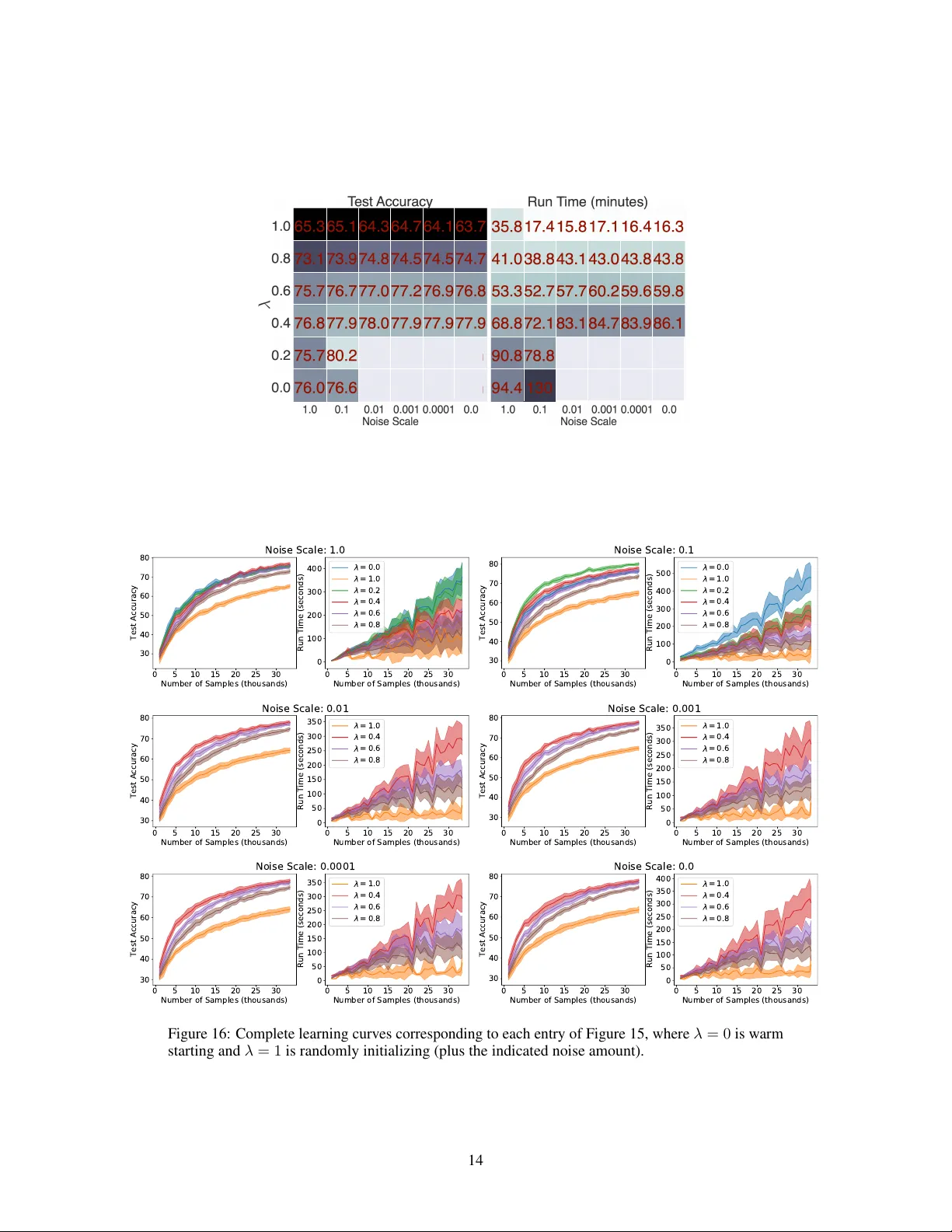
On W arm-Starting Neural Network T raining Jordan T . Ash Microsoft Research NYC ash.jordan@microsoft.com Ryan P . Adams Princeton Univ ersity rpa@princeton.edu Abstract In many real-w orld deployments of machine learning systems, data arri ve piece- meal. These learning scenarios may be passiv e, where data arriv e incrementally due to structural properties of the problem (e.g., daily financial data) or activ e, where samples are selected according to a measure of their quality (e.g., experi- mental design). In both of these cases, we are b uilding a sequence of models that incorporate an increasing amount of data. W e would like each of these models in the sequence to be performant and take advantage of all the data that are a vailable to that point. Con ventional intuition suggests that when solving a sequence of related optimization problems of this form, it should be possible to initialize using the solution of the pre vious iterate—to “warm start” the optimization rather than initialize from scratch—and see reductions in wall-clock time. Howe ver , in practice this warm-starting seems to yield poorer generalization performance than models that hav e fresh random initializations, ev en though the final training losses are similar . While it appears that some hyperparameter settings allow a practitioner to close this generalization gap, the y seem to only do so in regimes that damage the wall-clock gains of the warm start. Ne vertheless, it is highly desirable to be able to warm-start neural netw ork training, as it would dramatically reduce the resource usage associated with the construction of performant deep learning systems. In this work, we take a closer look at this empirical phenomenon and try to under - stand when and how it occurs. W e also provide a surprisingly simple trick that ov ercomes this pathology in sev eral important situations, and present experiments that elucidate some of its properties. 1 Introduction Although machine learning research generally assumes a fix ed set of training data, real life is more complicated. One common scenario is where a production ML system must be constantly updated with ne w data. This situation occurs in finance, online advertising, recommendation systems, fraud detection, and many other domains where machine learning systems are used for prediction and decision making in the real world [ 1 – 3 ]. When new data arriv e, the model needs to be updated so that it can be as accurate as possible and account for any domain shift that is occurring. As a concrete example, consider a large-scale social media website, to which users are constantly uploading images and text. The company requires up-to-the-minute predictiv e models in order to recommend content, filter out inappropriate media, and select advertisements. There might be millions of new data arri ving e very day , which need to be rapidly incorporated into production ML pipelines. It is natural in this scenario to imagine maintaining a single model that is updated with the latest data at regular cadence. Every day , for example, ne w training might be performed on the model with the updated, larger dataset. Ideally , this new training procedure is initialized from the parameters of yesterday’ s model, i.e., it is “warm-started” from those parameters rather than gi ven a fresh initialization. Such an initialization mak es intuiti ve sense: the data used yesterday are mostly the same as the data today , and it seems w asteful to thro w away all previous computation. For conv ex optimization problems, warm starting is widely used and highly successful (e.g., [ 1 ]), and the theoretical properties of online learning are well understood. 34th Conference on Neural Information Processing Systems (NeurIPS 2020), V ancouver , Canada. Figure 1: A comparison between ResNets trained using a warm start and a random initialization on CIF AR-10. Blue lines are models trained on 50% of CIF AR-10 for 350 epochs then trained on 100% of the data for a further 350 epochs. Orange lines are models trained on 100% of the data from the start. The tw o procedures produce sim- ilar training performance b ut dif fering test performance. Howe v er , warm-starting seems to hurt gen- eralization in deep neural networks. This is particularly troubling because w arm- starting does not damage training accuracy . Figure 1 illustrates this phenomenon. Three 18-layer ResNets ha ve been trained on the CIF AR-10 natural image classifi- cation task to create these figures. One was trained on 100% of the data, one was trained on 50% of the data, and a third warm-started model was trained on 100% of the data but initialized from the parame- ters found from the 50% trained model. All three achie ve the upper bound on training accuracy . Howe ver , the warm-started net- work performs worse on test samples than the network trained on the same data but with a ne w random initialization. Problematically , this phenomenon incentivizes performance-focused researchers and engineers to constantly retrain models from scratch, at potentially enormous financial and environmental cost [ 4 ]. This is an example of “Red AI” [5], disregarding resource consumption in pursuit of ra w predictiv e performance. The warm-start phenomenon has implications for other situations as well. In activ e learning, for example, unlabeled samples are abundant b ut labels are expensi ve: the goal is to identify maximally- informativ e data to ha ve labeled by an oracle and inte grated into the training set. It would be time efficient to simply warm-start optimization each time new samples are appended to the training set, but such an approach seems to damage generalization in deep neural networks. Although this phenomenon has not receiv ed much direct attention from the research community , it seems to be common practice in deep activ e learning to retrain from scratch after ev ery query step [ 6 , 7 ]; popular deep activ e learning repositories on Github randomly reinitialize models after ev ery selection. [ 8 , 9 ]. The ineffecti veness of warm-starting has been observed anecdotally in the community , but this paper seeks to examine its properties closely in controlled settings. Note that the findings in this paper are not inconsistent with e xtensiv e work on unsupervised pre-training [ 10 , 11 ] and transfer learning in the small-data and “few shot” regimes [ 12 – 15 ]. Rather here we are examining ho w to accelerate training in the large-data supervised setting in a w ay consistent with expectations from con ve x problems. This article is structured as follows. Section 2 examines the generalization gap induced by warm- starting neural networks. Section 3 surve ys approaches for improving generalization in deep learning, and shows that these techniques do not resolve the problem. In Section 4, we describe a simple trick that ov ercomes this pathology , and report on experiments that gi ve insights into its behavior in batch online learning and pre-training scenarios. W e defer our discussion of related work to Section 5, and include a statement on broad impacts in Section 6. 2 W arm Starting Damages Generalization In this section we provide empirical evidence that warm starting consistently damages generalization performance in neural networks. W e conduct a series of experiments across sev eral different architec- tures, optimizers, and image datasets. Our goal is to create simple, reproducible settings in which the warm-starting phenomenon is observed. 2.1 Basic Batch Updating Here we consider the simplest case of warm-starting, in which a single training dataset is partitioned into two subsets that are presented sequentially . In each series of experiments, we randomly segment the training data into two equally-sized portions. The model is trained to con ver gence on the first half, then is trained on the union of the two batches, i.e., 100% of the data. This is repeated for three classifiers: ResNet-18 [ 16 ], a multilayer perceptron (MLP) with three layers and tanh activ ations, and logistic regression. Models are optimized using either stochastic gradient descent (SGD) or the Adam variant of SGD [ 17 ], and are fitted to the CIF AR-10, CIF AR-100, and SVHN image data. All models are trained using a mini-batch size of 128 and a learning rate of 0.001, the smallest learning rate used in the learning schedule for fitting state-of-the-art ResNet models [ 16 ]. The effect of these parameters is in vestigated in Section 3. Presented results are on a held-out, randomly-chosen third of av ailable data. 2 R E S N E T R E S N E T M L P M L P L R L R C I F A R - 1 0 S G D A DA M S G D A D A M S G D A DA M R A N D O M I N I T 5 6 . 2 ( 1 . 0 ) 7 8 . 0 ( 0 . 6 ) 3 9 . 0 ( 0 . 2 ) 3 9 . 4 ( 0 . 1 ) 4 0 . 5 ( 0 . 6 ) 3 3 . 8 ( 0 . 6 ) W A R M S TART 5 1 . 7 ( 0 . 9 ) 7 4 . 4 ( 0 . 9 ) 3 7 . 4 ( 0 . 2 ) 3 6 . 1 ( 0 . 3 ) 3 9 . 6 ( 0 . 2 ) 3 3 . 3 ( 0 . 2 ) S V H N R A N D O M I N I T 8 9 . 4 ( 0 . 1 ) 9 3 . 6 ( 0 . 2 ) 7 6 . 5 ( 0 . 3 ) 7 6 . 7 ( 0 . 4 ) 2 8 . 0 ( 0 . 2 ) 2 2 . 4 ( 1 . 3 ) W A R M S TART 8 7 . 5 ( 0 . 7 ) 9 3 . 5 ( 0 . 4 ) 7 5 . 4 ( 0 . 1 ) 6 9 . 4 ( 0 . 6 ) 2 8 . 0 ( 0 . 3 ) 2 2 . 2 ( 0 . 9 ) C I F A R - 1 0 0 R A N D O M I N I T 1 8 . 2 ( 0 . 3 ) 4 1 . 4 ( 0 . 2 ) 1 0 . 3 ( 0 . 2 ) 1 1 . 6 ( 0 . 2 ) 1 6 . 9 ( 0 . 1 8 ) 1 0 . 2 ( 0 . 4 ) W A R M S TART 1 5 . 5 ( 0 . 3 ) 3 5 . 0 ( 1 . 2 ) 9 . 4 ( 0 . 0 ) 9 . 9 ( 0 . 1 ) 1 6 . 3 ( 0 . 2 8 ) 9 . 9 ( 0 . 3 ) T able 1 : V alidation percent accuracies for various opti- mizers and models for warm- started and randomly initial- ized models on indicated datasets. W e consider an 18-layer ResNet, three-layer multilayer perceptron (MLP), and logistic regression (LR). Figure 2: An online learning experiment for CIF AR-10 data using a ResNet. The horizontal axis shows the total number of samples in the training set a vailable to the learner . The generalization gap between warm-started and randomly-initialized models is significant. Our results (T able 1) indicate that gener- alization performance is damaged consis- tently and significantly for both ResNets and MLPs. This ef fect is more dramatic for CIF AR-10, which is considered rela- ti vely challenging to model (requiring, e.g., data augmentation), than for SVHN, which is considered easier . Logistic regression, which enjoys a con vex loss surf ace, is not significantly damaged by warm starting for any datasets. Figure 10 in the Appendix ex- tends these results and sho ws that the gap is in versely proportional to the fraction of data av ailable in the first round of training. This result is surprising. Even though MLP and ResNet optimization is non-con vex, con ventional intuition suggests that the warm-started solution should be close to the full-data solution and therefore a good initialization. One view on pre-training is that the initialization is a “prior” on weights; we often view prior distrib utions as arising from inference on old (or hypothetical) data and so this sort of pre-training should always be helpful. The generalization gap shown here creates a computational burden for real-life machine learning systems that must be retrained from scratch to perform well, rather than initialized from previous models. First-round results for T able 1 are in Appendix T able 2. 2.2 Online Learning A common real-world setting in volv es data that are being provided to the machine learning system in a stream. At every step, the learner is gi ven k ne w samples to append to its training data, and it updates its hypothesis to reflect the larger dataset. Financial data, social media data, and recommendation systems are common examples of scenarios where new samples are constantly arri ving. This paradigm is simulated in Figure 2, where we supply CIF AR-10 data, selected randomly without replacement, in batches of 1,000 to an 18-layer ResNet. W e examine two cases: 1) where the model is retrained from scratch after each batch, starting from a random initialization, and 2) where the model is trained to con ver gence starting from the parameters learned in the previous iteration. In both cases, the models are optimized with Adam, using an initial learning rate of 0.001. Each was run fi v e times with dif ferent random seeds and validation sets composed of a random third of av ailable data, reinitializing Adam’ s parameters at each step of learning. Figure 2 shows the trade-off between these two approaches. On the right are the training times: clearly , starting from the pre vious model is preferable and has the potential to vastly reduce computational costs and wall-clock time. Howe ver , as can be seen on the left, generalization performance is w orse in the warm-started situation. As more data arri ve, the gap in v alidation accuracy increases substantially . Means and standard de viations across fi ve runs are shown. Although this work focuses on image data, we find consistent results with other dataset and architecture choices (Appendix Figure 13). 3 Con ventional Appr oaches The design space for initializing and training deep neural network models is very large, and so it is important to e valuate whether there is some kno wn method that could be used to help warm-started training find good solutions. Put another way , a reasonable response to this problem is “Did you see whether X helped?” where X might be anything from batch normalization [ 18 ] to increasing mini- batch size [ 19 ]. This section tries to answer some of these questions and further empirically probe the warm-start phenomenon. Unless otherwise stated, experiments in this section use a ResNet-18 model trained using SGD with a learning rate of 0.001 on CIF AR-10 data. All experiments were run fi ve times to report means and standard de viations. No experiments in this paper use data augmentation or learning rate schedules, and all validation sets are a randomly-chosen third of the training data. 3 Figure 3 : A comparison between ResNets trained from both a warm start and a random initialization on CIF AR-10 for various hyperparam- eters. Orange dots are randomly- initialized models and blue dots are warm-started models. W arm-started models that perform roughly as well as randomly-initialized models of fer no benefit in terms of training time. 3.1 Is this an effect of batch size or learning rate? One might reasonably ask whether or not there e xist any hyperparameters that close the generalization gap between warm-started and randomly-initialized models. In particular , can setting a lar ger learning rate at either the first or second round of learning help the model escape to regions that generalize better? Can shrinking the batch size inject stochasticity that might improv e generalization [20, 21]? Figure 4: Left: V alidation accuracy as training pro- gresses on 50% of CIF AR-10. Right: V alidation ac- curacy damage, as percentage difference from random initialization, after training on 100% of the data. Each warm-started model was initialized by training on 50% of CIF AR data for the indicated number of epochs. Here we again consider a warm-started e x- periment of training on 50% of CIF AR-10 until con ver gence, then training on 100% of CIF AR-10 using the initial round of training as an initialization. W e explore all combi- nations of batch sizes { 16 , 32 , 64 , 128 } , and learning rates { 0 . 001 , 0 . 01 , 0 . 1 } , varying them across the three rounds of training. This allows for the possibility that there exist dif- ferent hyperparameters for the first stage of training that are better when used with a dif- ferent set after warm-starting. Each combina- tion is run with three random initializations. Figure 3 visualizes these results. Every resulting 100% model is shown from all three initializations and all combinations, with color indicating whether it was a random initialization or a warm-start. The horizontal axis sho ws the time to completion, excluding the pre-training time, and the vertical axis shows the resulting v alidation performance. Interestingly , we do find warm-started models that perform as well as randomly-initialized models, but the y are unable to do so while benefiting from their warm-started initialization. The training time for warm-started ResNet models that generalize as well as randomly-initialized models is roughly the same as those randomly-initialized models. That is, there is no computational benefit to using these warm-started initializations. It is worth noting that this plot does not capture the time or energy re- quired to identify hyperparameters that close the generalization gap; such hyperparameter searches are often the culprit in the resource footprint of deep learning [ 5 ]. W all-clock time is measured by assign- ing ev ery model identical resources, consisting of 50GB of RAM and an NVIDIA T esla P100 GPU. This increased fitting time occurs because w arm-started models, when using hyperparameters that generalize relativ ely well, seem to “forget” what was learned in the first round of training. Appendix Figure 11 provides evidence this phenomenon by computing the Pearson correlation between the weights of conv erged warm-started models and their initialization weights, again across various choices for learning rate and batch size, and comparing it to v alidation accurac y . Models that generalize well hav e little correlation with their initialization—there is a trend downward in accurac y with increasing correlation—suggesting that they ha ve forgotten what w as learned in the first round of training. Con versely , a similar plot for logistic regression sho ws no such relationship. 3.2 How quickly is generalization damaged? One surprising result in our inv estigation is that only a small amount of training is necessary to damage the validation performance of the warm-started model. Our hope was that warm-starting success might be achie ved by switching from the 50% to 100% phase before the first phase of training was completed. W e fit a ResNet-18 model on 50% of the training data, as before, and checkpointed its parameters ev ery fiv e epochs. W e then took each of these checkpointed models and used them as an initialization for training on 100% of those data. As shown in Figure 4, generalization is damaged e ven when initializing from parameters obtained by training on incomplete data for only a few epochs. 4 Figure 5: A two-phase experiment lik e those in Sections 2 and 3, where a ResNet is trained on 50% of CIF AR-10 and is then gi ven the remainder in the second round of training. Here we e xamine the av erage gradient norms separately corresponding to the initial 50% of data and the second 50% for models that are either warm-started or initialized with the shrink and perturb (SP) trick. Notice that in warm-started models, there is a drastic gap between these gradient norms. Our proposed trick balances these respectiv e magnitudes while still allowing models to benefit from their first round of training; i.e they fit training data much quicker than random initializations. 3.3 Is regularization helpful? Figure 6: W e fit a ResNet and MLP (with and without bias nodes) to CIF AR-10 and measure performance as a function of the shrinkage parameter λ . A common approach for impro ving generalization is to include a regularization penalty . Here we in vestigate three different approaches to re gularization: 1) basic L 2 weight penalties [ 22 ], 2) confidence-penalized training [ 23 ], and 3) adversarial training [ 24 ]. W e again take a ResNet fitted to 50% of av ailable training data and use its parameters to warm-start learning on 100% of the data. W e apply regu- larization in both rounds of training, and while it is helpful, regularization does not resolve the generalization gap in- duced by warm starting. Appendix T able 3 shows the result of these experiments for indicated regularization penalty sizes. Our e xperiments show that applying the same amount of regularization to randomly-initialized models still produces a better-generalizing classifier . 4 Shrink, P erturb, Repeat While the presented con ventional approaches do not remedy the warm-start problem, we ha ve identified a remarkably simple trick that ef ficiently closes the generalization gap. At each round of training t , when new samples are appended to the training set, we propose initializing the network’ s parameters by shrinking the weights found in the pre vious round of optimization tow ards zero, then adding a small amount of parameter noise. Specifically , we initialize each learnable parameter θ t i at training round t as θ t i ← λθ t − 1 i + p t , where p t ∼ N (0 , σ 2 ) and 0 < λ < 1 . Shrinking weights preserv es hypotheses. For network layers that use ReLU nonlinearities, shrink- ing parameters preserves the relative acti v ation at each layer . If bias terms and batch normalization are not used, the output of ev ery layer is a scaled version of its non-shrunken counterpart. In the last layer , which usually consists of a linear transformation followed by a softmax nonlinearity , shrinking parameters can be interpreted as increasing the entropy of the output distrib ution, ef fectiv ely diminish- ing the model’ s confidence. For no-bias, no-batchnorm ReLU models, while shrinking weights does not necessarily preserve the output f θ ( x ) they parametrize, it does preserve the learned hypothesis, i.e. arg max f θ ( x ) ; a simple proof is provided for completeness as Proposition 1 in the Appendix. For more sophisticated architectures, this property largely still holds: Figure 6 shows that for a ResNet, which includes batch normalization, only extreme amounts of shrinking are able to damage classifier performance. This is because batch normalization’ s internal estimates of mean and variance can compensate for the rescaling caused by weight shrinking. Even for a ReLU MLP that includes bias nodes, performance is surprisingly resilient to shrinking; classifier damage is done only for λ < 0 . 6 in Figure 6. Separately , note that when internal netw ork layers instead use sigmoidal activ ations, shrinking parameters mo ves them further from saturating regions, allo wing the model to more easily learn from new data. Shrink-perturb balances gradients. Figure 5 shows a visualization of av erage gradients during the second of a two-phase training procedure for a ResNet on CIF AR-10, like those discussed in Sections 2 and 3. W e plot the second phase of training, where gradient magnitudes are shown separately for the two halv es of the dataset. F or this experiment models are optimized with SGD, using a small learning rate to zoom in on this ef fect. Outside of this plot, experiments in this section use the Adam optimizer . 5 Figure 8 : Model performance as a function of λ and σ . Numbers indicate the av erage final perfor- mance and total train time for online learning ex- periments where ResNets are provided CIF AR-10 samples in sequence, 1,000 per round, and trained to con ver gence at each round. Note that the bot- tom left of this plot corresponds to pure random initializing while the top right corresponds to pure warm starting. Left : V alidation accuracy tends to improv e with more aggressive shrinking. Adding noise often improv es generalization. Right : Model train times increase with decreasing v alues of λ . This is expected, as decreasing λ widens the gap between shrink-perturb parameters and warm- started parameters. Noise helps models train more quickly . Unlabeled boxes correspond to initializa- tions too small for the model to reliably learn. For warm-started models, gradients from new , unseen data tend to be much larger magnitude than those from data the model has seen before. These imbalanced gradient contributions are known to be problematic for optimization in mutli-task learning scenarios [ 25 ], and suggest that under warm-started initializations the model does not learn in the same w ay as it would with randomly-initializied training [ 26 ]. W e find that remedying this imbalance without damaging what the model has already learned is key to ef ficiently resolving the generalization gap studied in this article. Shrinking the model’ s weights increases its loss, and correspondingly increases the magnitude of the gradient induced ev en by samples that hav e already been seen. Preposition 1 shows that in an L -layer ReLU network without bias nodes or batch normalization, shrinking weights by λ shrinks softmax inputs by λ L , rapidly increasing the entropy of the softmax distribution and the cross-entrop y loss. As shown in Figure 5, the loss increase caused by shrink perturb trick is able to balance gradient con- tributions between pre viously unseen samples and data on which the model has already been trained. The success of the shrink and perturb trick may lie in its ability to standardize gradients while preserving a model’ s learned hypothesis. W e could instead normalize gradient contributions by , for example, adding a significant amount of parameter noise, but this also damages the learned function. Consequently , this strategy drastically increases training time without fully closing the warm-start generalization gap (Appendix T able 4). As an alternativ e to shrinking all weights, we could try to increase the entrop y of the output distribution by shrinking only parameters in the last layer (Appendix Figure 14), or by regularizing the model’ s confidence while training (Appendix T able 3), b ut these are unable to resolve the warm-start problem. For sophisticated architectures especially , we find it is important to holistically modify parameters before training on new data. Figure 7: An online learning e xperiment v arying λ and keeping the noise scale fix ed at 0 . 01 . Note that λ = 1 corresponds to fully-warm-started initializations and λ = 0 corresponds to fully-random initializations. The proposed trick with λ = 0 . 6 performs identically to randomly initializing in terms of validation accurac y , but trains much more quickly . Interestingly , smaller values of λ are e ven able to outperform random initialization while still training faster . The perturbation step, adding noise after shrinking, improv es both training time and generalization performance. The trade-off between relative v alues of λ and σ is studied in Figure 8. Note that in this figure, and in this section generally , we refer to the “noise scale” rather than to σ . In practice, we add noise by adding parameters from a scaled, randomly-initialized network, to compen- sate for the fact that many random initial- ization schemes use dif ferent variances for different kinds of parameters. Figure 7 demonstrates the effecti veness of this trick. Lik e before, we present a passiv e online learning experiment where 1,000 CIF AR-10 samples are supplied to a ResNet in sequence. At each round we can either reinitialize network parameters from scratch or warm start, initializing them to 6 Figure 9 : Pre-trained models fitted to a varying fraction of the indicated dataset. W e compare these warm- started, pre-trained models to ran- domly initialized and shrink-perturb initialized counterparts, trained on the same fraction of tar get data. The relati ve performance of warm- starting and randomly initializing varies, but shrink-perturb performs at least as well as the best strategy . those found in the previous round of optimization. As expected, we see that warm-started models train faster b ut generalize worse. Howe ver , if we instead initialize parameters using the shrink and perturb trick, we are able to both close this generalization gap and significantly speed up training. Appendix Sections 8.2.1-8.2.6 present extensi ve results v arying λ and noise scale, e xperimenting with dataset type, model architecture, and L 2 regularization, all showing the same ov erall trend. Indeed, we notice that shrink-perturb parameters that better balance gradient contributions better remedy the warm-start problem. That said, we find that one does not need to shrink very aggressiv ely to adequately enough correct gradients and efficiently close the w arm-start generalization gap. 4.1 The shrink and perturb trick and regularization Exercising the shrink and perturb trick at e very step of SGD would be very similar to applying an aggressiv e, noisy L 2 regularization. That is, shrink-perturbing every step of optimization yields the SGD update θ i ← λ ( θ i − η ∂ L ∂ θ i ) + p for loss L , weight θ i , and learning rate η , making the shrinkage term λ behav e like a weight decay parameter . It is natural to ask, then, ho w does this trick compare with weight decay? Appendix Figure 12 sho ws that in non-w arm-started en vironments, where we just hav e a static dataset, the iterative application of the shrink-perturb trick results in mar ginally impro ved performance. These experiments fit a ResNet to conv ergence on 100% of CIF AR-10 data, then shrink and perturb weights before repeating the process, resulting in a modest performance improvement. W e can conclude that the shrink-perturb trick has two benefits. Most significantly , it allows us to quickly fit high-performing models in sequential en vironments without having to retrain from scratch. Separately , it offers a slight regularization benefit, which in combination with the first property sometimes allo ws shrink-perturb models to generalize ev en better than randomly-initialized models. This L 2 regularization benefit is not enough to explain the success of the shrink-perturb trick. As Appendix T able 3 demonstrates, L 2 -regularized models are still vulnerable to the warm-start general- ization g ap. Appendix Sections 8.2.5 and 8.2.6 show that we are able to mitigate this performance gap with the shrink and perturb trick ev en when models are being aggressively re gularized (regularization penalties any lar ger prev ent networks from being able to fit the training data) with weight decay . 4.2 The shrink and perturb trick and pre-training Despite successes on a variety of tasks, deep neural networks still generally require large training sets to perform well. For problems where only limited data are a vailable, it has become popular to warm-start learning using parameters obtained by training on a dif ferent but related dataset [ 14 , 27 ]. T ransfer and “few-shot” learning in this form has seen success in computer vision and NLP [28]. The experiments we perform here, ho wev er , imply that when the second problem is not data-limited, this transfer learning approach deteriorates model quality . That is, at some point, the pre-training trans- fer learning approach is similar to warm-starting under domain shift, and generalization should suffer . W e demonstrate this phenomenon by first training a ResNet-18 to con ver gence on one dataset, then using that solution to warm-start a model trained on a varying fraction of another dataset. When only a small portion of target data are used, this is essentially the same as the pre-training transfer learning approach. As the proportion increases, the problem turns into what we have described here as warm starting. Figure 9 sho ws the result of this experiment, and it appears to support our intuition. Often, when the second dataset is small, warm starting is helpful, but there is frequently a crossov er point where better generalization would be achie ved by training from scratch on that fraction of the target data. Sometimes, when source and tar get datasets are dissimilar , it would better to randomly initialize regardless of the amount of tar get data av ailable. 7 The exact point at which this crossover occurs (and whether it happens at all) depends not just on model type but also on the statistical properties of the data in question; it cannot be easily predicted. W e find that shrink-perturb initialization, howe ver , allo ws us to av oid having to mak e such a prediction: shrink-perturbed models perform at least as well as warm-started models when pre-training is the most performant strategy and as well as randomly-initialized models when it is better to learn from scratch. Figure 9 displays this effect for λ = 0 . 3 and noise scale 0.0001. Comprehensi ve shrink-perturb settings for this scenario are giv en in Appendix Section 8.2.7, all showing similar results. 5 Discussion and Research Surrounding the W arm Start Pr oblem W arm-starting is well understood for con vex models lik e linear classifiers [ 29 ] and SVMs [ 30 , 31 ], and has been e xplored for neural netw orks to improv e optimization on a fixed dataset [ 32 ]. Excluding the shrink-perturb trick, it does not appear that generally applicable techniques exist for deep neural networks that remedy the warm-start problem, so models are typically retrained from scratch [ 6 , 33 ]. There has been a v ariety of w ork in closely related areas, howe ver . For example, in analyzing “critical learning periods, ” researchers sho w that a network initially trained on blurry images then on sharp images is unable to perform as well as one trained from scratch on sharp images, drawing a parallel between human vision and computer vision [ 26 ]. W e sho w that this phenomenon is more general, with test performance damaged ev en when first and second datasets are drawn from identical distributions. Initialization. The problem of warm starting is closely related to the rich literature on initialization of neural network training “from scratch”. Indeed, ne w insights into what makes an effecti ve initialization hav e been critical to the revi v al of neural networks as machine learning models. While there ha ve been se v eral proposed methods for initialization [ 34 , 35 , 10 , 36 , 37 ], this body of literature primarily concerns itself with initializations that are high-quality in the sense that they allow for quick and reliable model training. That is, these methods are typically b uilt with training performance in mind rather than generalization performance. W ork relating initialization to generalization suggests that netw orks whose weights hav e mov ed far from their initialization are less likely to generalize well compared with ones that ha ve remained relativ ely nearby [ 38 ]. Here we hav e shown with e xperimental results that warm-started networks that have less in common with their initializations seem to generalize better than those that have more (Appendix Figure 11). So while it is not surprising that there exist initializations that generalize poorly , it is surprising that warm starts are in that class. Still, before retraining, our proposed solution brings parameters closer their initial values than they would be if just warm starting, suggesting some relationship between generalization and distance from initialization. Generalization. The warm-start problem is fundamentally about generalization performance, which has been extensi vely studied both theoretically and empirically within the context of deep learning. These articles ha ve inv estigated generalization by studying classifier margin [ 39 , 40 ], loss ge- ometry [ 41 , 19 , 42 ], and measurements of complexity [ 43 , 44 ], sensitivity [ 45 ], or compressiblity [ 46 ]. These approaches can be seen as attempting to measure the intricacy of the hypothesis learned by the network. If two models are both consistent for the same training data, the one representing the simpler concept is more likely to generalize well. W e kno w that networks trained with SGD are implicitly regularized [ 20 , 21 ], suggesting that standard training of neural networks incidentally finds low-comple xity solutions. It’ s possible, then, that the initial round of training disqualifies solutions that would most naturally e xplain the the data. If so, by balancing gradient contributions, the shrink and perturb trick seems to make these solutions accessible again. Pre-training . As pre viously discussed, the warm-start problem is very similar to the idea of unsupervised and supervised pre-training [ 47 , 11 , 10 , 48 ]. Under that paradigm, learning where limited labeled data are a vailable is aided by first training on related data. The warm start problem, howe ver , is not about limited labeled data in the second round of training. Instead, the goal of warm starting is to hasten the time required to fit a neural network by initializing using a similar supervised problem without damaging generalization. Our results suggest that while warm-starting is beneficial when labeled data are limited, it actually damages generalization to warm-start in data-rich situations. Concluding thoughts. This article presented the challenges of w arm-starting neural network training and proposed a simple and powerful solution. While warm-starting is a problem that the community seems somewhat aware of anecdotally , it does not seem to hav e been directly studied. W e believe that this is a major problem in important real-life tasks for which neural networks are used, and it speaks directly to the resources consumed by training such models. 8 6 Broader Impact The shrink and perturb trick allo ws models to be ef ficiently updated without sacrificing generalization performance. In the absence of this method, achieving best-possible performance requires neural networks to be randomly-initialized each time new data are appended to the training set. As mentioned earlier , this requirement can cost significant computational resources, and as a result, is partially responsible for the deleterious en vironmental ramifications studied in recent years [4, 5]. Additionally , the enormous computational expense of retraining models from scratch disproportion- ately burdens research groups without access to abundant computational resources. The shrink and perturb trick lowers this barrier , democratizing research in sequential learning with neural networks. 7 Funding Disclosur e and Competing Interests This work was partially funded by NSF IIS-2007278 and by a Siemens FutureMakers graduate student fellowship. RP A is on the board of directors at Cambridge Machines Ltd. and is a scientific advisor to Manifold Bio. References [1] Xinran He, Junfeng P an, Ou Jin, T ianbing Xu, Bo Liu, T ao Xu, Y anxin Shi, Antoine Atallah, Ralf Herbrich, Stuart Bowers, et al. Practical lessons from predicting clicks on ads at Facebook. In W orkshop on Data Mining for Online Advertising , pages 1–9. ACM, 2014. [2] Badrish Chandramouli, Justin J Lev andoski, Ahmed Eldawy , and Mohamed F Mokbel. Stream- Rec: a real-time recommender system. In International Confer ence on Management of Data , pages 1243–1246. A CM, 2011. [3] Ludmila I Kunche v a. Classifier ensembles for detecting concept change in streaming data: Overvie w and perspectiv es. In 2nd W orkshop SUEMA , volume 2008, pages 5–10, 2008. [4] Emma Strubell, Ananya Ganesh, and Andrew McCallum. Energy and policy considerations for deep learning in NLP. In Annual Meeting of the Association for Computational Linguistics , 2019. [5] Roy Schwartz, Jesse Dodge, Noah A Smith, and Oren Etzioni. Green AI. arXiv pr eprint arXiv:1907.10597 , 2019. [6] Ozan Sener and Silvio Sav arese. Acti ve learning for con volutional neural networks: A core-set approach. In International Conference on Learning Repr esentations , 2018. [7] Jordan T Ash, Chicheng Zhang, Akshay Krishnamurthy , John Langford, and Alekh Agar - wal. Deep batch activ e learning by diverse, uncertain gradient lower bounds. arXiv pr eprint arXiv:1906.03671 , 2019. [8] Rostamiz. https://github.com/ej0cl6/deep- active- learning , 2017–2019. [9] K uan-Hao Huang. https://github.com/ej0cl6/deep- active- learning , 2018–2019. [10] Dumitru Erhan, Y oshua Bengio, Aaron Courville, Pierre-Antoine Manzagol, Pascal V incent, and Samy Bengio. Why does unsupervised pre-training help deep learning? Journal of Machine Learning Resear ch , 11(Feb):625–660, 2010. [11] Y oshua Bengio. Deep learning of representations for unsupervised and transfer learning. In International Confer ence on Unsupervised and T ransfer Learning W orkshop , pages 17–37. JMLR, 2011. [12] Oriol V inyals, Charles Blundell, T imothy Lillicrap, and Daan W ierstra. Matching networks for one shot learning. In Advances in Neural Information Pr ocessing Systems , pages 3630–3638, 2016. [13] Jake Snell, K evin Swersky , and Richard Zemel. Prototypical networks for fe w-shot learning. In Advances in Neural Information Pr ocessing Systems , pages 4077–4087, 2017. 9 [14] Chelsea Finn, Pieter Abbeel, and Sergey Le vine. Model-agnostic meta-learning for fast adapta- tion of deep netw orks. In International Conference on Machine Learning , pages 1126–1135. JMLR. org, 2017. [15] Jordan T Ash, Robert E Schapire, and Barbara E Engelhardt. Unsupervised domain adaptation using approximate label matching. arXiv preprint , 2016. [16] Kaiming He, Xiangyu Zhang, Shaoqing Ren, and Jian Sun. Deep residual learning for image recognition. In IEEE Confer ence on Computer V ision and P attern Recognition , pages 770–778, 2016. [17] Diederik P Kingma and Jimmy Ba. Adam: A method for stochastic optimization. International Confer ence on Learning Repr esentations , 2014. [18] Serge y Ioffe and Christian Sze gedy . Batch normalization: Accelerating deep network training by reducing internal cov ariate shift. arXiv preprint , 2015. [19] Nitish Shirish Keskar , Dheev atsa Mudigere, Jorge Nocedal, Mikhail Smelyanskiy , and Ping T ak Peter T ang. On lar ge-batch training for deep learning: Generalization gap and sharp minima. International Confer ence on Learning Repr esentations , 2016. [20] Y uanzhi Li, T engyu Ma, and Hongyang Zhang. Algorithmic regularization in over -parameterized matrix sensing and neural networks with quadratic acti vations. pages 75:2–47, 2018. [21] Suriya Gunasekar , Blake E W oodworth, Srinadh Bhojanapalli, Behnam Ne yshabur , and Nati Srebro. Implicit regularization in matrix factorization. In Advances in Neural Information Pr ocessing Systems , pages 6151–6159, 2017. [22] Anders Krogh and John A Hertz. A simple weight decay can improve generalization. In Advances in Neural Information Pr ocessing Systems , pages 950–957, 1992. [23] Gabriel Pereyra, George T ucker , Jan Chorowski, Ł ukasz Kaiser, and Geoffre y Hinton. Reg- ularizing neural netw orks by penalizing confident output distrib utions. arXiv preprint arXiv:1701.06548 , 2017. [24] Christian Szegedy , W ojciech Zaremba, Ilya Sutske ver , Joan Bruna, Dumitru Erhan, Ian Good- fellow , and Rob Fergus. Intriguing properties of neural networks. In International Confer ence on Learning Repr esentations , 2014. [25] T ianhe Y u, Saurabh K umar , Abhishek Gupta, Ser gey Le vine, Karol Hausman, and Chelsea Finn. Gradient surgery for multi-task learning. arXiv pr eprint arXiv:2001.06782 , 2020. [26] Alessandro Achille, Matteo Rovere, and Stefano Soatto. Critical learning periods in deep networks. In International Conference on Learning Repr esentations , 2018. [27] Alex Nichol and John Schulman. Reptile: a scalable metalearning algorithm. arXiv pr eprint arXiv:1803.02999 , 2, 2018. [28] Lili Mou, Zhao Meng, Rui Y an, Ge Li, Y an Xu, Lu Zhang, and Zhi Jin. How transferable are neural networks in NLP applications? In Empirical Methods in Natural Langua ge Pr ocessing , pages 478–489, 2016. [29] Bo-Y u Chu, Chia-Hua Ho, Cheng-Hao Tsai, Chieh-Y en Lin, and Chih-Jen Lin. W arm start for parameter selection of linear classifiers. In International Confer ence on Knowledge Discovery and Data Mining , pages 149–158. A CM, 2015. [30] Dennis DeCoste and Kiri W agstaff. Alpha seeding for support v ector machines. In International Confer ence on Knowledge Discovery and Data Mining , pages 345–349. A CM, 2000. [31] Zeyi W en, Bin Li, Ramamohanarao K otagiri, Jian Chen, Y awen Chen, and Rui Zhang. Im- proving effi ciency of SVM k -fold cross-validation by alpha seeding. In Thirty-F irst AAAI Confer ence on Artificial Intelligence , 2017. [32] Ilya Loshchilov and Frank Hutter . Sgdr: Stochastic gradient descent with warm restarts. arXiv pr eprint arXiv:1608.03983 , 2016. 10 [33] Pranav Shyam, W ojciech Ja ´ sko wski, and Faustino Gomez. Model-based activ e exploration. In International Confer ence on Machine Learning , pages 5779–5788, 2018. [34] Ilya Sutske ver , James Martens, George Dahl, and Geof frey Hinton. On the importance of initial- ization and momentum in deep learning. In International Conference on Machine Learning , pages 1139–1147, 2013. [35] Rupesh K Sri vasta va, Klaus Gref f, and J ¨ urgen Schmidhuber . T raining very deep networks. In Advances in Neural Information Pr ocessing Systems , pages 2377–2385, 2015. [36] Xavier Glorot and Y oshua Bengio. Understanding the dif ficulty of training deep feedforward neural networks. In International Conference on Artificial Intelligence and Statistics , pages 249–256, 2010. [37] Kaiming He, Xiangyu Zhang, Shaoqing Ren, and Jian Sun. Delving deep into rectifiers: Sur- passing human-level performance on ImageNet classification. In IEEE International Confer ence on Computer V ision , pages 1026–1034, 2015. [38] V aishnavh Nagarajan and J Zico K olter . Generalization in deep networks: The role of distance from initialization. In Neural Information Pr ocessing Systems , 2017. [39] Peter L Bartlett, Dylan J F oster , and Matus J T elgarsky . Spectrally-normalized mar gin bounds for neural networks. In Advances in Neural Information Pr ocessing Systems , pages 6240–6249, 2017. [40] Colin W ei, Jason D Lee, Qiang Liu, and T engyu Ma. On the margin theory of feedforward neural networks. arXiv preprint , 2018. [41] Sepp Hochreiter and J Schmidhuber . Flat minima. Neural Computation , 9(1):1–42, 1997. [42] Hao Li, Zheng Xu, Gavin T aylor , Christoph Studer , and T om Goldstein. V isualizing the loss landscape of neural nets. In Advances in Neural Information Pr ocessing Systems , pages 6389–6399, 2018. [43] Chiyuan Zhang, Samy Bengio, Moritz Hardt, Benjamin Recht, and Oriol V inyals. Understanding deep learning requires rethinking generalization. In International Confer ence on Learning Repr esentations , 2017. [44] T engyuan Liang, T omaso Poggio, Alexander Rakhlin, and James Stokes. Fisher -Rao metric, geometry , and complexity of neural networks. pages 888–896, 2017. [45] Roman Nov ak, Y asaman Bahri, Daniel A Abolafia, Jef frey Pennington, and Jascha Sohl- Dickstein. Sensitivity and generalization in neural netw orks: an empirical study . In International Confer ence on Learning Repr esentations , 2018. [46] W enda Zhou, V ictor V eitch, Morgane Austern, Ryan P Adams, and Peter Orbanz. Non-v acuous generalization bounds at the ImageNet scale: a P A C-Bayesian compression approach. In International Confer ence on Learning Repr esentations , 2019. [47] Hengduo Li, Bharat Singh, Mahyar Najibi, Zuxuan W u, and Larry S Davis. An analysis of pre-training on object detection. arXiv preprint , 2019. [48] Y oshua Bengio, Pascal Lamblin, Dan Popovici, and Hugo Larochelle. Greedy layer-wise training of deep networks. In Advances in neural information processing systems , pages 153–160, 2007. 11 8 A ppendix Proposition 1. Consider a neural network f θ trained to pr edict one of k classes and paramatrized by weight matrices θ = ( W 1 , W 2 , .., W L ) . Using the ReLU nonlinearity σ ( z ) = max(0 , z ) and softmax( z ) i = e z i / P k j =1 e z j , let f θ ( x ) = softmax( W L · σ ( W L − 1 · .. · σ ( W 2 · σ ( W 1 · x )))) . Then, for λ > 0 and input x , arg max f θ ( x ) = arg max f λθ ( x ) . Pr oof. Observe that σ ( λz ) = λσ ( z ) ∀ λ > 0 . Then, arg max f λθ ( x ) = arg max softmax( λW L · σ ( λW L − 1 · .. · σ ( λW 2 · σ ( λW 1 · x )))) = arg max softmax( λ L W L · σ ( W L − 1 · .. · σ ( W 2 · σ ( W 1 · x )))) = arg max softmax( W L · σ ( W L − 1 · .. · σ ( W 2 · σ ( W 1 · x )))) = arg max f θ ( x ) 8.1 Appendix T ables T able 2: V alidation percent accuracies for v arious optimizers and models for the first round of warm-started training, i.e. training on half of the training data a vailable in T able 1. W e consider an 18-layer ResNet, three-layer multilayer perceptron (MLP), and logistic regression (LR) as our classifiers. V alidation sets are a randomly-chosen third of the training data. Standard deviations are indicated parenthetically . R E S N E T R E S N E T M L P M L P L R L R S G D A DA M S G D A DA M S G D A DA M C I FA R - 1 0 4 1 . 7 ( 7 . 9 ) 7 0 . 5 ( 1 . 6 ) 3 7 . 2 ( 0 . 2 ) 3 6 . 0 ( 0 . 2 ) 3 7 . 9 ( 0 . 2 ) 3 1 . 8 ( 0 . 7 ) S V H N 8 5 . 9 ( 0 . 3 ) 9 2 . 3 ( 0 . 2 ) 7 2 . 5 ( 0 . 4 ) 6 7 . 5 ( 0 . 3 ) 2 7 . 1 ( 0 . 3 ) 2 2 . 2 ( 0 . 7 ) C I FA R - 1 0 0 1 0 . 6 ( 1 . 6 ) 3 1 . 5 ( 0 . 7 ) 1 0 . 3 ( 0 . 2 ) 1 0 . 5 ( 0 . 3 ) 1 5 . 4 ( 0 . 2 1 ) 9 . 3 ( 0 . 3 ) T able 3: V alidation percent accuracies for v arious optimizers and models for the first round of warm-started training, i.e. training on half of the training data a vailable in T able 1. W e consider an 18-layer ResNet, three-layer multilayer perceptron (MLP), and logistic regression (LR) as our classifiers. V alidation sets are a randomly-chosen third of the training data. Standard deviations are indicated parenthetically . L 2 1 × 10 − 1 1 × 10 − 2 1 × 10 − 3 1 × 10 − 4 R I 7 2 . 7 ( 4 . 2 ) 5 5 . 4 ( 2 . 7 ) 5 4 . 6 ( 2 . 4 ) 5 5 . 1 ( 3 . 4 ) W S 6 3 . 9 ( 6 . 4 ) 5 1 . 2 ( 2 . 7 ) 5 0 . 5 ( 1 . 8 ) 5 0 . 4 ( 1 . 3 ) A DV E R S A R I A L R I 5 4 . 8 ( 1 . 3 ) 5 5 . 1 ( 1 . 5 ) 5 5 . 3 ( 1 . 4 ) 5 5 . 6 ( 0 . 9 ) W S 5 2 . 4 ( 1 . 0 ) 5 2 . 6 ( 1 . 5 ) 5 2 . 7 ( 1 . 2 ) 5 0 . 4 ( 1 . 4 ) C O N FI D E N C E R I 5 3 . 1 ( 1 . 9 ) 5 5 . 8 ( 1 . 3 ) 5 5 . 4 ( 1 . 2 ) 5 5 . 9 ( 1 . 4 ) W S 5 0 . 3 ( 0 . 7 ) 5 0 . 0 ( 3 . 8 ) 5 1 . 2 ( 1 . 2 ) 4 9 . 3 ( 1 . 2 ) T able 4: V alidation accuracies and warm-started model train times (minutes). Adding noise at the indicated standard de viations improves generalization, b ut not to the point of performing as well as randomly-initialized models. Better-generalizing w arm-started models take ev en more time to train than their randomly-initialized peers, which on av erage achiev e 55.2% accuracy in 34.0 minutes. 1 × 10 − 2 1 × 10 − 3 1 × 10 − 4 1 × 10 − 5 0 Accuracy 54.4 (0.9) 53.5 (1.0) 52.9 (1.0) 49.9 (1.6) 50.8 (1.8) T rain T ime 165.3 (3.9) 38.0 (1.33) 16.5 (1.3) 14.6 (91.0) 13.6 (0.4) T able 5: V alidation percent accuracies for various datasets for last layer only warm-starting (LL), last layer warm starting follo wed by full network training (LL+WS), warm started (WS) and randomly initialized (RI) models on various indicated datasets. LL LL+WS WS RI CIF AR-10 48.8 (1.8) 50.9 (1.5) 52.5 (0.3) 56.0 (1.2) SVHN 86.0 (0.6) 88.2 (0.2) 87.5 (0.7) 89.4 (0.1) CIF AR-100 16.4 (0.5) 16.5 (0.6) 15.5 (0.3) 18.2 (0.3) 12 8.2 Appendix Figures Figure 10: W arm-started ResNet generalization as a function of the fraction of total data av ailable in the first round of training. Models are trained on the indicated fraction of CIF AR-10 training data until con v ergence, then trained again on 100% of CIF AR-10 data to produce this figure. When the initial data used to warm-start training more ov erlaps with the second round of training data, the generalization gap is less se vere. Figure 11: V alidation accurac y as a function of the correlation between the warm-start initializa- tion and the solution found after training for a large number of hyperparameter settings. Left : W arm-started logistic regressors often remem- ber their initialization. Right : W arm-started ResNets that perform well do not retain much information from the initial round of training. Figure 12: The result of fitting a ResNet on 100% of CIF AR-10 to con ver gence for twenty rounds and applying the shrink-perturb trick after each. Here we show four v ersions of that experiment for the indicated λ and a noise scaling of 0.01. Iterativ e application has a slight regularization ef fect. Figure 13: An online learning experiment using a two-layer bidirectional RNN trained on the IMDB movie re vie w sentiment classification dataset. Samples are supplied iid in batches of 1,000. Like with other experiments, warm start- ing ( λ = 1 ) performs significantly worse than randomly initializing ( λ = 0 ). Shrink-perturb initialization closes this generalization gap. 0 5 10 15 20 25 30 Number of Samples (thousands) 30 40 50 60 70 Test Accuracy Noise Scale 0.1 0 5 10 15 20 25 30 Number of Samples (thousands) 30 40 50 60 70 Test Accuracy Noise Scale 0.01 warm fresh = 0 . 2 = 0 . 4 = 0 . 8 Figure 14: An online learning experiment using a ResNet on CIF AR-10 data. Data are supplied iid in batches of 1,000. Here, instead of shrinking and per- turbing ev ery weight in the model, we modify only those in the last layer . Models modified this way , unlike the shrink-perturb trick we present, which modifies e very parameter in the network, these re- trained models are unable to outperform e ven purely warm-started models. 13 8.2.1 Batch Online Learning Results for a ResNet-18 on CIF AR-10 This section sho ws results of a shrink and perturb online learning e xperiment with a ResNet-18 on CIF AR-10 data, iterativ ely supplying batches of 1,000 to the model and training it to con ver gence. Figure 15: A verage performance resulting from using the shrink and perturb trick with varying choices for λ and noise scale. Final accuracies and train times. Missing numbers correspond to initializations that were too small to be trained. The bottom left entry is a pure random initialization while the top right is a pure warm start. 0 5 10 15 20 25 30 Number of Samples (thousands) 30 40 50 60 70 80 Test Accuracy 0 5 10 15 20 25 30 Number of Samples (thousands) 0 100 200 300 400 Run Time (seconds) = 0 . 0 = 1 . 0 = 0 . 2 = 0 . 4 = 0 . 6 = 0 . 8 Noise Scale: 1.0 0 5 10 15 20 25 30 Number of Samples (thousands) 30 40 50 60 70 80 Test Accuracy 0 5 10 15 20 25 30 Number of Samples (thousands) 0 100 200 300 400 500 Run Time (seconds) = 0 . 0 = 1 . 0 = 0 . 2 = 0 . 4 = 0 . 6 = 0 . 8 Noise Scale: 0.1 0 5 10 15 20 25 30 Number of Samples (thousands) 30 40 50 60 70 80 Test Accuracy 0 5 10 15 20 25 30 Number of Samples (thousands) 0 50 100 150 200 250 300 350 Run Time (seconds) = 1 . 0 = 0 . 4 = 0 . 6 = 0 . 8 Noise Scale: 0.01 0 5 10 15 20 25 30 Number of Samples (thousands) 30 40 50 60 70 80 Test Accuracy 0 5 10 15 20 25 30 Number of Samples (thousands) 0 50 100 150 200 250 300 350 Run Time (seconds) = 1 . 0 = 0 . 4 = 0 . 6 = 0 . 8 Noise Scale: 0.001 0 5 10 15 20 25 30 Number of Samples (thousands) 30 40 50 60 70 80 Test Accuracy 0 5 10 15 20 25 30 Number of Samples (thousands) 0 50 100 150 200 250 300 350 Run Time (seconds) = 1 . 0 = 0 . 4 = 0 . 6 = 0 . 8 Noise Scale: 0.0001 0 5 10 15 20 25 30 Number of Samples (thousands) 30 40 50 60 70 80 Test Accuracy 0 5 10 15 20 25 30 Number of Samples (thousands) 0 50 100 150 200 250 300 350 400 Run Time (seconds) = 1 . 0 = 0 . 4 = 0 . 6 = 0 . 8 Noise Scale: 0.0 Figure 16: Complete learning curves corresponding to each entry of Figure 15, where λ = 0 is warm starting and λ = 1 is randomly initializing (plus the indicated noise amount). 14 8.2.2 Batch Online Learning Results for a ResNet-18 on SVHN Here we show an online learning e xperiment with a ResNet-18 on SVHN data, iterativ ely supplying batches of 1,000 to the model and training it to con ver gence. Figure 17: A verage fianl accuracies and train times when using the shrink and perturb trick with v ary- ing choices for λ and noise scale. Missing numbers correspond to initializations that were too small to be trained. The bottom left entry is a pure random initialization while the top right is a pure w arm start. 0 10 20 30 40 50 Number of Samples (thousands) 30 40 50 60 70 80 90 Test Accuracy 0 10 20 30 40 50 Number of Samples (thousands) 0 50 100 150 200 250 300 350 Run Time (seconds) = 0 . 0 = 1 . 0 = 0 . 2 = 0 . 4 = 0 . 6 = 0 . 8 Noise Scale: 1.0 0 10 20 30 40 50 Number of Samples (thousands) 40 50 60 70 80 90 Test Accuracy 0 10 20 30 40 50 Number of Samples (thousands) 0 100 200 300 400 Run Time (seconds) = 0 . 0 = 1 . 0 = 0 . 2 = 0 . 4 = 0 . 6 = 0 . 8 Noise Scale: 0.1 0 10 20 30 40 50 Number of Samples (thousands) 30 40 50 60 70 80 90 Test Accuracy 0 10 20 30 40 50 Number of Samples (thousands) 0 50 100 150 200 250 Run Time (seconds) = 1 . 0 = 0 . 4 = 0 . 6 = 0 . 8 Noise Scale: 0.01 0 10 20 30 40 50 Number of Samples (thousands) 30 40 50 60 70 80 90 Test Accuracy 0 10 20 30 40 50 Number of Samples (thousands) 0 50 100 150 200 250 Run Time (seconds) = 1 . 0 = 0 . 4 = 0 . 6 = 0 . 8 Noise Scale: 0.001 0 5 10 15 20 25 30 Number of Samples (thousands) 30 40 50 60 70 80 Test Accuracy 0 5 10 15 20 25 30 Number of Samples (thousands) 0 50 100 150 200 250 300 350 Run Time (seconds) = 1 . 0 = 0 . 4 = 0 . 6 = 0 . 8 Noise Scale: 0.0001 0 5 10 15 20 25 30 Number of Samples (thousands) 30 40 50 60 70 80 Test Accuracy 0 5 10 15 20 25 30 Number of Samples (thousands) 0 50 100 150 200 250 300 350 400 Run Time (seconds) = 1 . 0 = 0 . 4 = 0 . 6 = 0 . 8 Noise Scale: 0.0 Figure 18: Complete learning curves corresponding to each entry of Figure 17, where λ = 0 is warm starting and λ = 1 is randomly initializing (plus the indicated noise amount). 15 8.2.3 Batch Online Learning Results for an MLP on CIF AR-10 (no batch normalization) Here we show an online learning experiment, training an MLP consisting of three layers, ReLU activ ations, and 100-dimensional hidden layers (no batch normalization) on CIF AR-10 data. Figure 19: Final accuracies and train times resulting from using the shrink and perturb trick with v ary- ing choices for λ and noise scale. Missing numbers correspond to initializations that were too small to be trained. The bottom left entry is a pure random initialization while the top right is a pure w arm start. 0 5 10 15 20 25 30 Number of Samples (thousands) 32.5 35.0 37.5 40.0 42.5 45.0 47.5 Test Accuracy 0 5 10 15 20 25 30 Number of Samples (thousands) 0 200 400 600 800 Run Time (seconds) = 0 . 0 = 1 . 0 = 0 . 2 = 0 . 4 = 0 . 6 = 0 . 8 Noise Scale: 0.1 0 5 10 15 20 25 30 Number of Samples (thousands) 34 36 38 40 42 44 46 48 Test Accuracy 0 5 10 15 20 25 30 Number of Samples (thousands) 0 100 200 300 400 500 Run Time (seconds) = 1 . 0 = 0 . 4 = 0 . 6 = 0 . 8 Noise Scale: 0.01 0 5 10 15 20 25 30 Number of Samples (thousands) 32 34 36 38 40 42 44 46 Test Accuracy 0 5 10 15 20 25 30 Number of Samples (thousands) 0 100 200 300 400 500 Run Time (seconds) = 1 . 0 = 0 . 4 = 0 . 6 = 0 . 8 Noise Scale: 0.001 0 5 10 15 20 25 30 Number of Samples (thousands) 34 36 38 40 42 44 46 Test Accuracy 0 5 10 15 20 25 30 Number of Samples (thousands) 0 100 200 300 400 500 Run Time (seconds) = 1 . 0 = 0 . 4 = 0 . 6 = 0 . 8 Noise Scale: 0.0001 0 5 10 15 20 25 30 Number of Samples (thousands) 34 36 38 40 42 44 46 48 Test Accuracy 0 5 10 15 20 25 30 Number of Samples (thousands) 0 100 200 300 400 500 600 700 Run Time (seconds) = 1 . 0 = 0 . 4 = 0 . 6 = 0 . 8 Noise Scale: 0.0 Figure 20: Complete learning curves corresponding to each entry of Figure 19, where λ = 0 is warm starting and λ = 1 is randomly initializing (plus the indicated noise amount). 16 8.2.4 Batch Online Learning Results for an MLP on SVHN (no batch normalization) Here we show an online learning experiment, training an MLP consisting of three layers, ReLU activ ations, and 100-dimensional hidden layers (no batch normalization) on SVHN data. Figure 21: A verage final accuracies and train times resulting from using the shrink and perturb trick with varying choices for λ and noise scale. W e iterativ ely supply batches of 1,000 to the model and train it to con ver gence. Missing numbers correspond to initializations that were too small to be trained. The bottom left entry is a pure random initialization while the top right is a pure warm start. 0 10 20 30 40 50 Number of Samples (thousands) 50 55 60 65 70 75 80 Test Accuracy 0 10 20 30 40 50 Number of Samples (thousands) 0 100 200 300 400 500 Run Time (seconds) = 1 . 0 = 0 . 4 = 0 . 6 = 0 . 8 Noise Scale: 0.01 0 10 20 30 40 50 Number of Samples (thousands) 50 55 60 65 70 75 80 Test Accuracy 0 10 20 30 40 50 Number of Samples (thousands) 0 100 200 300 400 500 Run Time (seconds) = 1 . 0 = 0 . 4 = 0 . 6 = 0 . 8 Noise Scale: 0.001 0 10 20 30 40 50 Number of Samples (thousands) 50 55 60 65 70 75 80 Test Accuracy 0 10 20 30 40 50 Number of Samples (thousands) 0 100 200 300 400 500 Run Time (seconds) = 1 . 0 = 0 . 4 = 0 . 6 = 0 . 8 Noise Scale: 0.0001 0 10 20 30 40 50 Number of Samples (thousands) 50 55 60 65 70 75 80 Test Accuracy 0 10 20 30 40 50 Number of Samples (thousands) 0 100 200 300 400 500 Run Time (seconds) = 1 . 0 = 0 . 4 = 0 . 6 = 0 . 8 Noise Scale: 0.0 Figure 22: Complete learning curves corresponding to each entry of Figure 21, where λ = 0 is warm starting and λ = 1 is randomly initializing (plus the indicated noise amount). 17 8.2.5 Batch Online Learning Results for a ResNet-18 on CIF AR-10 with weight decay Here we sho w an online learning experiment, with a ResNet-18 on CIF AR-10 data, iteratively supplying batches of 1,000 to the model and training it to con ver gence with a weight decay penalty of .001. Note that this is aggressiv e regularization—increasing weight decay by an order of magnitude results in models that cannot reliably fit the training data. Figure 23: A verage final performance and run times resulting from using the shrink and perturb trick with v arying choices for λ and noise scale. Missing numbers correspond to initializations that were too small to be trained. The bottom left entry is a pure random initialization while the top right is a pure warm start. 0 5 10 15 20 25 30 Number of Samples (thousands) 30 40 50 60 70 80 Test Accuracy 0 5 10 15 20 25 30 Number of Samples (thousands) 0 50 100 150 200 250 300 350 400 Run Time (seconds) = 1 . 0 = 0 . 4 = 0 . 6 = 0 . 8 Noise Scale: 0.01 0 5 10 15 20 25 30 Number of Samples (thousands) 30 40 50 60 70 80 Test Accuracy 0 5 10 15 20 25 30 Number of Samples (thousands) 0 50 100 150 200 250 300 350 Run Time (seconds) = 1 . 0 = 0 . 4 = 0 . 6 = 0 . 8 Noise Scale: 0.001 0 5 10 15 20 25 30 Number of Samples (thousands) 30 40 50 60 70 80 Test Accuracy 0 5 10 15 20 25 30 Number of Samples (thousands) 0 100 200 300 400 Run Time (seconds) = 1 . 0 = 0 . 4 = 0 . 6 = 0 . 8 Noise Scale: 0.0001 0 5 10 15 20 25 30 Number of Samples (thousands) 30 40 50 60 70 80 Test Accuracy 0 5 10 15 20 25 30 Number of Samples (thousands) 0 50 100 150 200 250 300 350 400 Run Time (seconds) = 1 . 0 = 0 . 4 = 0 . 6 = 0 . 8 Noise Scale: 0.0 Figure 24: Complete learning curves corresponding to each entry of Figure 23, where λ = 0 is warm starting and λ = 1 is randomly initializing (plus the indicated noise amount). 18 8.2.6 Batch Online Learning Results for a ResNet-18 on SVHN with weight decay Here we show an online learning experiment, with a ResNet-18 on SVHN data, iteratively supplying batches of 1,000 to the model and training it to con vergence with a weight decay penalty of .001. Note that this is aggressive re gularization—increasing weight decay by an order of magnitude results in models that cannot reliably fit the training data. Figure 25: A verage final accuracies and train times resulting from using the shrink and perturb trick with v arying choices for λ and noise scale. Here we show an online learning experiment with a ResNet- 18 on SVHN data, iterativ ely supplying batches of 1,000 to the model and training it to conv ergence with a weight decay of .001. Missing numbers correspond to initializations that were too small to be trained. The bottom left entry is a pure random initialization while the top right is a pure warm start. 0 10 20 30 40 50 Number of Samples (thousands) 30 40 50 60 70 80 90 Test Accuracy 0 10 20 30 40 50 Number of Samples (thousands) 0 100 200 300 400 500 Run Time (seconds) = 0 . 0 = 1 . 0 = 0 . 2 = 0 . 4 = 0 . 6 = 0 . 8 Noise Scale: 1.0 0 10 20 30 40 50 Number of Samples (thousands) 30 40 50 60 70 80 90 Test Accuracy 0 10 20 30 40 50 Number of Samples (thousands) 0 100 200 300 400 500 600 Run Time (seconds) = 0 . 0 = 1 . 0 = 0 . 2 = 0 . 4 = 0 . 6 = 0 . 8 Noise Scale: 0.1 0 10 20 30 40 50 Number of Samples (thousands) 30 40 50 60 70 80 90 Test Accuracy 0 10 20 30 40 50 Number of Samples (thousands) 0 50 100 150 200 250 Run Time (seconds) = 1 . 0 = 0 . 4 = 0 . 6 = 0 . 8 Noise Scale: 0.01 0 10 20 30 40 50 Number of Samples (thousands) 30 40 50 60 70 80 90 Test Accuracy 0 10 20 30 40 50 Number of Samples (thousands) 0 50 100 150 200 250 300 Run Time (seconds) = 1 . 0 = 0 . 4 = 0 . 6 = 0 . 8 Noise Scale: 0.001 0 10 20 30 40 50 Number of Samples (thousands) 30 40 50 60 70 80 90 Test Accuracy 0 10 20 30 40 50 Number of Samples (thousands) 0 50 100 150 200 250 300 Run Time (seconds) = 1 . 0 = 0 . 4 = 0 . 6 = 0 . 8 Noise Scale: 0.0001 0 10 20 30 40 50 Number of Samples (thousands) 30 40 50 60 70 80 90 Test Accuracy 0 10 20 30 40 50 Number of Samples (thousands) 0 50 100 150 200 250 300 Run Time (seconds) = 1 . 0 = 0 . 4 = 0 . 6 = 0 . 8 Noise Scale: 0.0 Figure 26: Complete learning curves corresponding to each entry of Figure 25, where λ = 0 is warm starting and λ = 1 is randomly initializing (plus the indicated noise amount). 19 8.2.7 Shrink and P erturb f or Pre-T raining In this section we sho w the effect of applying the shrink and perturb trick at various noise scales in pre-training scenarios like those shown in Figure 9. In each experiment we pre-train a ResNet-18 on one dataset and then train to con ver gence on the the indicated fraction of a target dataset. 0.0 0.2 0.4 0.6 0.8 1.0 75 80 85 90 95 Accuracy (SVHN) Pretraining with CIFAR 0.0 0.2 0.4 0.6 0.8 1.0 10 20 30 40 50 Accuracy (CIFAR100) Pretraining with CIFAR 0.0 0.2 0.4 0.6 0.8 1.0 40 50 60 70 80 Accuracy (CIFAR) Pretraining with SVHN 0.0 0.2 0.4 0.6 0.8 1.0 Available fraction of CIFAR100 10 20 30 40 50 Accuracy (CIFAR100) Pretraining with SVHN warm fresh = 0 . 2 = 0 . 4 = 0 . 6 = 0 . 8 0.0 0.2 0.4 0.6 0.8 1.0 Available fraction of CIFAR 40 50 60 70 80 Accuracy (CIFAR) Pretraining with CIFAR100 0.0 0.2 0.4 0.6 0.8 1.0 Available fraction of SVHN 70 75 80 85 90 95 Accuracy (SVHN) Pretraining with CIFAR100 Figure 27: Shrink and perturb pre-train plots for various shrinkage perameters λ and noise scale 1e-5. 0.0 0.2 0.4 0.6 0.8 1.0 75 80 85 90 95 Accuracy (SVHN) Pretraining with CIFAR 0.0 0.2 0.4 0.6 0.8 1.0 10 20 30 40 50 Accuracy (CIFAR100) Pretraining with CIFAR 0.0 0.2 0.4 0.6 0.8 1.0 40 50 60 70 80 Accuracy (CIFAR) Pretraining with SVHN 0.0 0.2 0.4 0.6 0.8 1.0 Available fraction of CIFAR100 10 20 30 40 50 Accuracy (CIFAR100) Pretraining with SVHN warm fresh = 0 . 2 = 0 . 4 = 0 . 6 = 0 . 8 0.0 0.2 0.4 0.6 0.8 1.0 Available fraction of CIFAR 40 50 60 70 80 Accuracy (CIFAR) Pretraining with CIFAR100 0.0 0.2 0.4 0.6 0.8 1.0 Available fraction of SVHN 70 75 80 85 90 95 Accuracy (SVHN) Pretraining with CIFAR100 Figure 28: Shrink and perturb pre-train plots for various shrinkage perameters λ and noise scale 1e-4. 0.0 0.2 0.4 0.6 0.8 1.0 75 80 85 90 95 Accuracy (SVHN) Pretraining with CIFAR 0.0 0.2 0.4 0.6 0.8 1.0 10 20 30 40 50 Accuracy (CIFAR100) Pretraining with CIFAR 0.0 0.2 0.4 0.6 0.8 1.0 40 50 60 70 80 Accuracy (CIFAR) Pretraining with SVHN 0.0 0.2 0.4 0.6 0.8 1.0 Available fraction of CIFAR100 10 20 30 40 50 Accuracy (CIFAR100) Pretraining with SVHN warm fresh = 0 . 2 = 0 . 4 = 0 . 6 = 0 . 8 0.0 0.2 0.4 0.6 0.8 1.0 Available fraction of CIFAR 40 50 60 70 80 Accuracy (CIFAR) Pretraining with CIFAR100 0.0 0.2 0.4 0.6 0.8 1.0 Available fraction of SVHN 70 75 80 85 90 95 Accuracy (SVHN) Pretraining with CIFAR100 Figure 29: Shrink and perturb pre-train plots for various shrinkage perameters λ and noise scale 1e-3. 20 0.0 0.2 0.4 0.6 0.8 1.0 75 80 85 90 95 Accuracy (SVHN) Pretraining with CIFAR 0.0 0.2 0.4 0.6 0.8 1.0 10 20 30 40 50 Accuracy (CIFAR100) Pretraining with CIFAR 0.0 0.2 0.4 0.6 0.8 1.0 40 50 60 70 80 Accuracy (CIFAR) Pretraining with SVHN 0.0 0.2 0.4 0.6 0.8 1.0 Available fraction of CIFAR100 10 20 30 40 50 Accuracy (CIFAR100) Pretraining with SVHN warm fresh = 0 . 2 = 0 . 4 = 0 . 6 = 0 . 8 0.0 0.2 0.4 0.6 0.8 1.0 Available fraction of CIFAR 40 50 60 70 80 Accuracy (CIFAR) Pretraining with CIFAR100 0.0 0.2 0.4 0.6 0.8 1.0 Available fraction of SVHN 70 75 80 85 90 95 Accuracy (SVHN) Pretraining with CIFAR100 Figure 30: Shrink and perturb pre-train plots for various shrinkage perameters λ and noise scale 1e-2. 0.0 0.2 0.4 0.6 0.8 1.0 75 80 85 90 95 Accuracy (SVHN) Pretraining with CIFAR 0.0 0.2 0.4 0.6 0.8 1.0 10 20 30 40 50 Accuracy (CIFAR100) Pretraining with CIFAR 0.0 0.2 0.4 0.6 0.8 1.0 40 50 60 70 80 Accuracy (CIFAR) Pretraining with SVHN 0.0 0.2 0.4 0.6 0.8 1.0 Available fraction of CIFAR100 10 20 30 40 50 Accuracy (CIFAR100) Pretraining with SVHN warm fresh = 0 . 2 = 0 . 4 = 0 . 6 = 0 . 8 0.0 0.2 0.4 0.6 0.8 1.0 Available fraction of CIFAR 40 50 60 70 80 Accuracy (CIFAR) Pretraining with CIFAR100 0.0 0.2 0.4 0.6 0.8 1.0 Available fraction of SVHN 70 75 80 85 90 95 Accuracy (SVHN) Pretraining with CIFAR100 Figure 31: Shrink and perturb pre-train plots for various shrinkage perameters λ and noise scale 1e-1. 9 Companion Figur es Figure 32: An online learning experiment, using CIF AR-10 data supplied to a ResNet in batches of 10000, using a learning rate schedule and SGD instead of a fixed learning rate with Adam. Figure 33: A companion to Figure 11, sho wing validation accurac y as a function of dif ferent correlation measurements between warm-started model final weights and initializations. 21