Signal-Based Properties of Cyber-Physical Systems: Taxonomy and Logic-based Characterization

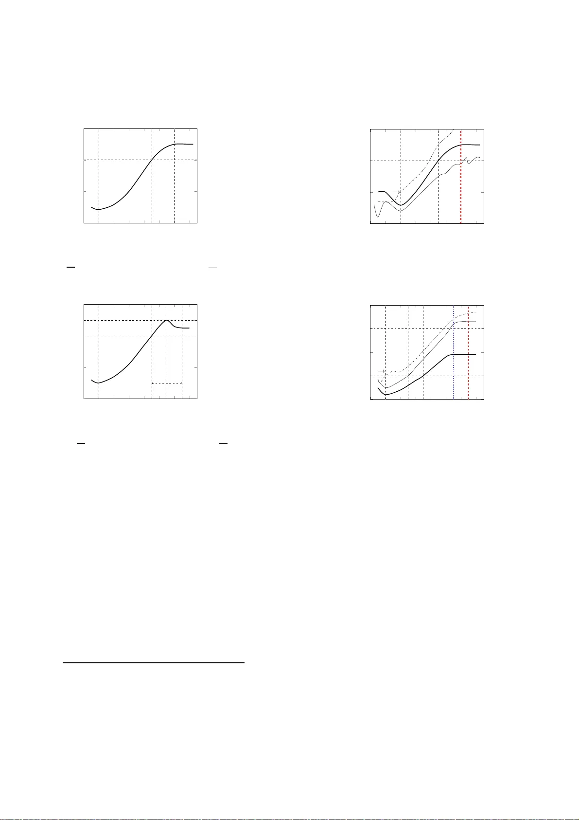
Signal -Based Prop erties of Cyb er-P h ysical System s: T axonomy and Logic-ba sed Character izati on Chaima Boufaied a, ∗ , Maris Jukss 1 , Domenico Bianculli a , Lionel Claude Briand a,b , Y ago Isasi Parache c a Inter disciplinary Centr e for Se curity, R eliability and T ru st (SnT), University of Luxembo ur g, Luxemb our g b Scho ol of EECS, U ni v ersity of Ott awa, Canada c LuxSp ac e S` arl Abstract The b ehavior of a cy ber -physical system (CPS) is usually deﬁned in terms o f the input and output signals pro cessed by sensors and actuators. Requirements sp eciﬁcations of CPSs ar e typically expr essed using signal-bas ed tempo ral prope r ties. Expressing suc h requirements is c hallenging, b ecause of (1) the many features that ca n b e used to characterize a sig nal b ehavior; (2) the broad v aria tion in express iveness of the sp eciﬁcation langua ges (i.e., temp oral logics) used for deﬁning signal-based tempor al prop erties. Thus, system and soft ware engineers need eﬀectiv e guidance on selecting appr opriate signal behavior t ypes and an adequate speciﬁca tion languag e , based on the type of requirements they ha ve to deﬁne. In this pap er, we present a taxo nomy of the v arious types of signal- ba sed prop er ties and provide, for each t yp e, a co mprehensive and detailed desc r iption as well as a formaliza tion in a temp ora l logic . F urthermor e, we review the ex pressiveness of sta te-of-the-art signal- based temp or al logics in terms o f the prop erty types ident iﬁed in the taxo nomy . Mo reov er, we r ep o rt o n the application of o ur tax onomy to classify the require- men ts speciﬁca tions of an industria l case study in the aer ospace domain, in o rder to assess the feasibility of using the prop erty types included in our taxo nomy a nd the completeness of the latter. Keywor d s: signals, signal-based prop erties, tempo ral logic, taxonomy 1. In tro duction Cyb er-physical systems (CP Ss) a re systems characterized by a complex interw eaving o f ha rdware a nd softw are [1]. They a re widely used in man y safety-critical doma ins (e.g., aerospa ce, automotive, medical) where v alidation and veriﬁcation (V&V) activities [2] o f the s ystem’s in tended functionality play a crucial role to guarantee the reliability and s afety of the system. A t ypical CPS consists of a mix o f analo g and digital comp onents, such as se nsors, actuator s , and control units, which pr o cess input and output signa ls . System engineers sp ecify the desired system be havior by deﬁning requirements in terms of the sig nals obtained from these comp onents. Such requirements ca n be sp eciﬁed using signal-b ase d temp o r al pr op erties , which characterize the expected behavior o f signa ls . F o r example, a prop erty may require that a signal must no t exhibit an a brupt increa se of a mplitude (i.e., a spike or bump) within a certain time interv al, or that the signal shall manifest an oscilla tory b ehavior with a particular per io d. Expressing requirements in terms of signa l-based temp oral prop er ties poses a num ber of challenges for system and softw are engineer s. First, a sig na l b ehavior (e.g., a spike) can b e characterized using a num ber o f ∗ Corresp onding author Email addr esses: chai ma.boufaied @uni.lu (Chaima Boufaied), maris.jukss@ gmail.com (Maris Jukss), domenico .bianculli@ uni.lu (Domenico Bianculli), lionel.briand@u ni.lu (Lionel Cl aude Briand), Isasi@luxspace.l u (Y ago Isasi Parac he) 1 This w ork was done while the author was aﬃliated with the Interdisciplinary Cen tre for Security , Reliabil ity and T rust (SnT), Universit y of Luxem b ourg, Luxembourg. Pr eprint submitte d to Elsevier De c emb e r 29, 2020 features (e.g., amplitude, slop e, width); for example, a total of 16 diﬀer en t features (and eight parameters) hav e b een iden tiﬁed in the literature [3] to detect (and thus c haracter ize) a spik e in a signal. Engineers may decide to choose v ar ious s ubsets of features; without prop er guidelines fo r selec ting the features most appropria te in a certain context and without their pre cise characteriza tion, the resulting speciﬁca tion of a signal b ehavior may become ambiguous or incons is ten t. The second challenge is r elated to the expr essiveness of the sp eciﬁcation languages us ed for deﬁning signal- ba sed temp or a l pro per ties. Starting from the se minal work on STL [4] (Signal T empo ral Log ic), there have b een s everal prop osals of lang uages that ex tend more traditional temp ora l logic s like L TL (Linear T emp oral Logic) to supp ort the spe ciﬁcation o f sig nal- based behaviors. Such languages hav e diﬀer e n t levels of expressiveness when it comes to describing certa in signal behaviors. F or example, S TL cannot b e used to express prop erties (like those rela ted to oscillatory behaviors) that require to reference the concrete v a lue of a signal at an instant in which a certain prop erty was satisﬁed [5]. This mea ns that engineer s need guida nce to carefully s elect the langua ge to us e for deﬁning signal-bas ed pr op erties, based on the type of r equirements they ar e go ing to deﬁne, the expr essiveness o f the candidate speciﬁcation languages , and the av ailabilit y of suitable to ols (e.g., trace chec k er) for each language. W e remark that these challenges for the sp eciﬁcation of signal-ba sed temp oral pro per ties hav e implica- tions also in terms of V&V. The lack o f precise descriptions o f signal behaviors (and their features) and the use of sp eciﬁcation la nguages with limited express iveness, may le ad engineers to r esort to manual checking (e.g., v is ual insp ection of signal wa vef orms) of prop erties on signa ls. Although an a nomalous s pike in ampli- tude can b e easily sp otted by visual insp ection of the wav eform o f a sig nal that is mo stly stable, man ually detecting complex signal b ehaviors on w a veforms with in tricate shap es is a cum be rsome and er ror-pr one pro cess. In this pap er, we tackle these tw o challenges by prop os ing a taxo nomy of the most common types of signal-bas ed temp oral prop er ties and a log ic-based c harac terization of such prop erties. Based on industrial exp erience a nd a thoroug h review of the litera ture, our go al is to provide system and softw are engine e r s, as well as resear ch ers working on CPSs, with a r eference g uide to systematically identif y a nd c haracter iz e signal b ehaviors, to supp ort b oth requirements sp eciﬁcation and V&V activities. More sp eciﬁca lly , we address the ﬁrst challenge by providing, through the taxono my , a co mpr ehensive and deta iled description of the diﬀerent types of signal-based b ehaviors, with each prope r t y type precisely c haracter ized in terms of a tempo ral logic . As a r esult, an engineer ca n b e guided by the precise characteriza tion of the pro p er ty types included in our tax onomy , to derive—from an informal r equirements sp eciﬁcation—a forma l sp eciﬁcatio n of a pr o pe rty , which can then b e used in the context of V& V a ctivities (e.g., a s test or acle). W e take on the second challenge by revie w ing the expres siveness of the ma in temp oral logics that hav e b een prop os ed in the literature for sp ecifying signal-bas ed tempo ral prop e rties (i.e., S TL , STL* [5], SFO [6] - Signal First-Order Logic), in terms o f the pr o pe r ty types iden tiﬁed in the tax onomy . In this way , w e ca n guide enginee r s to choose a speciﬁca tion formalism based on their needs in terms of prop erty types to expr e s s. W e dev elop ed our taxonomy of signal-base d prop erties bas e d on practica l exp erience in analyzing tem- po ral req uirements in CPS do mains like the aero space industry , and by reviewing the literature in the area of v eriﬁcation of cyber -physical systems, starting from the recent s urvey of spec iﬁca tion formalisms in reference [2]. W e identiﬁed and included in our taxonomy the following prope r ty types: • Dat a assertion , which s p eciﬁes cons traints on the signal v alue; • S ignal b e havior , repr esenting a signal behavior in terms of a par ticular wa veform, such as spikes and oscillations; • Rel ationship b etwe en signals , a t yp e tha t includes funct ional r elatio nship properties, based on the application of a tr ansformation (e.g., diﬀerentiation) on sig na ls, and or der r elationship pr op erties, stating constraints on the or der of even ts/states related to signal behaviors. The or der r elationshi p t yp e also includes prop er ties descr ibing the tr ansie nt b ehavio r of a signa l when changing from the current v alue to a new target v alue (i.e., rising/falling, ov ersho oting/unders ho oting b ehaviors). F or each o f these types, we provide a lo gic-based characterization using SFO and a lso discuss alternative formalizations —w he n applicable —us ing also STL a nd STL* . In this w ay , we are a ble to re po rt on the ex - 2 pressiveness of state-of-the-a rt tempor al log ic s with resp ect to the prop erty types included in o ur taxono m y: SFO is the only la nguage among the three we conside r ed in which we can expres s al l the pr op erty typ es of our taxonomy . W e also rep ort on the a pplication of our tax onomy to classify the re q uirements speciﬁcations of a n industrial case study in the aerospa ce doma in. Through this case study we show: • The fea sibility of expres s ing r e quirements s pec iﬁc a tions of a real-world CPS using the pro per t y t ype s included in our taxonomy . Indeed, in the v ast ma jority of the ca ses, the mapping from a speciﬁca tion written in English to its corr esp onding pr op erty type deﬁned in the taxonomy was straig htforward. • The c ompleteness of our taxonomy: all requirements sp eciﬁcations of the case study could b e deﬁned using the prop erty types included in our taxo nomy . T o summarize, the main contributions of this pa per ar e: • a taxo nomy o f signal-bas ed prop er ties; • a log ic-based c harac ter ization of the v arious prop erty types included in the taxo no m y; • a disc us sion on the expr essiveness of state- o f-the-art temp oral log ic s with resp ect to the prop erty t yp es included in our taxonomy; • the application of our taxono m y to classify the r equirements sp eciﬁca tions o f an industrial ca se study in the aeros pa ce domain. The res t of the pa per is structured a s follows. Section 2 provides background concepts o n signals and tempo ral logics for signal-ba sed pro per ties. Section 3 illustrates our tax onomy of signal-ba s ed prop er ties and pr ovides a logic-ba sed character ization of ea ch prop erty type. In section 4 we discuss the expressiveness of state-of-the-art temp or a l log ics with res pect to the pro per t y t ype s included in our taxonomy . Section 5 presents the applicatio n o f our taxonomy to a n industr ial case study . Sectio n 6 discusses how the paper contributions can supp or t the resear ch communit y a nd prac titioners. Section 7 discuss es related work. Section 8 concludes the paper , providing directio ns for future work. 2. Bac kground 2.1. Signals A ﬁnite leng th s ig nal s over a domain D is a function s : T → D , where T is the time domain and D is an application-de p endent v a lue domain. In the context of CPSs, we need to diﬀerentiate b et ween analo g , discr ete , and digital signals [7]. An analog signal is a signal that is c ontin uous b oth in the time and in the v alue domains. The time domain T of a n analog signa l is th us the set o f non-negative r eal n umbers R ≥ 0 and the v alue domain D is the set o f r eal n umbers R . Mor e formally , we deﬁne an analo g signal s a as s a : T → R . The do ma in of deﬁnition of s a is the interv al I s a = [0 , r ), with r ∈ Q ≥ 0 ; the length of s a is deﬁned as | s a | = r ; undeﬁned signal v a lues are denoted by s a ( t ) = ⊥ , ∀ t ≥ | s a | . In a dis c rete signal, the v alue domain is contin uous whereas the time domain is the se t of natural n umbers N . More s peciﬁc a lly , a discrete signal can be obtained from a n ana lo g signal through sampling , which is the pro cess of co n verting the contin uous-time domain of a signal to a discrete- time domain. Thr oughout this pro cess, the analog signal is read at a regular time in terv al ∆ called the sampling interval . The resulting discretized signal s dsc can be repre sent ed by the v a lues of an analog signal s a read at the following time po in ts: 0 , ∆ , 2 × ∆ , . . . , k × ∆. A digital signal has the set of natur a l num b e rs N as time domain and a ﬁnite discrete set a s v alue domain. Such a sig nal ca n b e obtained from a discrete signal b y quantization , whic h is the pro cess of transforming contin uous v alues in to their ﬁnite discr ete approximations. In the rest of the pap er we will consider analog signa ls, simply denoted by s , unles s a sp eciﬁc signal type is explicitly mentioned. This choice is motiv ated by the con text in whic h this work has been developed, which 3 is the domain of CP S [8]. In such a domain, mo del-driven engineering is used throug hout the developmen t pro cess and simulation is used for design-time testing of system mo dels; s im ulation mo dels (e.g., those deﬁned in Simu link ® ) capture b oth co ntin uous a nd discre te system b ehaviors and, when executed, pro duce traces containing analo g sig nals [9]. 2.2. T emp or a l L o gi cs for Signal-b ase d Pr op erties In this section, we provide a brief introduction to the main temp ora l logics that hav e b een pr op osed in the liter ature for sp ecifying signal-based temp oral pro pe r ties. They w ill b e used in the next s ection to present the forma liz ation o f sig nal-based prop erties. 2.2.1. Signal T emp or al L o gi c ( STL ) STL [4] has b een one of the ﬁrst pro po sals of a temp or al logic for the sp eciﬁcation of temp oral pr op erties ov er dense-time (i.e., T = R ≥ 0 ), real-v alued signals. Let Π b e a ﬁnite set of a tomic pro po sitions, X b e a ﬁnite set of real v ariables, and I be an interv al 2 [ a, b ] ov er R with a, b ∈ Q ≥ 0 such that 0 ≤ a < b . The syntax of STL with bo th futur e a nd p ast o per ators [10] is deﬁned by the following gr a mmar: ϕ ::= p | x ∼ c | ¬ ϕ | ϕ 1 ∨ ϕ 2 | ϕ 1 U I ϕ 2 | ϕ 1 S I ϕ 2 where p ∈ Π, x ∈ X , ∼∈ { <, ≤ , = , ≥ , > } , c ∈ R , U I is the metric “ Until ” ope r ator, and S I is the metric “ Sinc e ” op er a tor. Additional tempor al op er a tors can be derived using the usual conv entions; for exa mple, “ Eventual ly ” F I ϕ ≡ ⊤ U I ϕ ; “ Glob al ly ” G I ϕ ≡ ¬ F I ¬ ϕ ; “ Onc e (Eventu al ly in the Past) ” P I ϕ ≡ ⊤ S I ϕ ; “ Historic al ly ” H I ϕ ≡ ¬ P I ¬ ϕ . The semantics of STL is deﬁned through a satisfaction rela tion ( s, t ) | = STL ϕ , which indicates tha t signal s satisﬁes formula ϕ sta r ting fro m po s ition t in the signal. The sa tisfaction relation is deﬁned inductively as follows: ( s, t ) | = STL p iﬀ p holds on s in t, for p ∈ Π ( s, t ) | = STL x ∼ c iﬀ x ∼ c holds on s in t, for x ∈ X and c ∈ R ( s, t ) | = STL ¬ ϕ iﬀ ( s, t ) 6| = STL ϕ ( s, t ) | = STL ϕ 1 ∨ ϕ 2 iﬀ ( s, t ) | = STL ϕ 1 or ( s, t ) | = STL ϕ 2 ( s, t ) | = STL ϕ 1 U [ a,b ] ϕ 2 iﬀ ∃ t ′ . ( t ′ ∈ [ t + a, t + b ] and ( s, t ′ ) | = STL ϕ 2 and ∀ t ′′ . ( t ′′ ∈ [ t, t ′ ] and ( s, t ′′ ) | = STL ϕ 1 )) ( s, t ) | = STL ϕ 1 S [ a,b ] ϕ 2 iﬀ ∃ t ′ . ( t ′ ∈ [ t − a, t − b ] and ( s, t ′ ) | = STL ϕ 2 and ∀ t ′′ . ( t ′′ ∈ [ t, t ′ ] and ( s, t ′′ ) | = STL ϕ 1 )) W e say that a signal s satisﬁes an STL formula ϕ iﬀ ( s, 0) | = STL ϕ . Several extensions of STL hav e b een prop osed in the literature. F or exa mple, STL/PSL [11] adds an analog lay er to STL that enables the application of (low-lev el) signal op era tions; xSTL [12] adds supp ort for Timed Regular Expre s sions [13]. The STL expres s ions tha t we will pr e sent in the res t o f the pap er can be written in the s a me form also in STL/PSL or xSTL since they only rely on the core op erators of STL . 2.2.2. STL* STL* [5] is a n extension of STL that adds a signal-v alue fr e ezing op era tor that binds the v alue of a signal to a precise instant of time. Let J b e a ﬁnite index set (e.g., the set { 1 , . . . , n } , n ∈ N ) and let the function t ∗ : J → [0 , | s | ] be the fr ozen time ve ctor ; the i-th fro z en time can then b e referred to with t ∗ i = t ∗ ( i ). As in the cas e of STL , let Π b e a ﬁnite set of atomic prop ositions , X be a ﬁnite set o f rea l v ariables, and I be an in terv al [ a, b ] over R with a, b ∈ Q ≥ 0 such that 0 ≤ a < b . The syntax of STL* is deﬁned by the following grammar : ϕ ::= p | x ∼ c | ¬ ϕ | ϕ 1 ∨ ϕ 2 | ϕ 1 U I ϕ 2 | ∗ i [ ϕ ] 2 The restriction on the non-punctual interv al I for STL has been li f ted i n reference [10 ] . 4 where p ∈ Π, x ∈ X , ∼∈ { <, ≤ , = , ≥ , > } , c ∈ R , U I is the metric “ Un t il ” o pe r ator, and ∗ i is the unar y signal-v alue freezing op erator for all i ∈ J . Additiona l op erator s like Eventual ly and Glob al ly can b e deﬁned as done above for STL . The sema n tics of STL* is deﬁned throug h a s a tisfaction rela tio n ( s, t, t ∗ ) | = STL ∗ ϕ , which indicates that signal s satisﬁes form ula ϕ star ting from p osition t in the sig nal, tak ing into account the frozen time v ector t ∗ ∈ [0 , | s | ] J . The satisfaction relation is deﬁned inductively as follows: ( s, t, t ∗ ) | = STL ∗ p iﬀ p holds on s in t, for p ∈ Π , with the fro zen time vector t ∗ ( s, t, t ∗ ) | = STL ∗ x ∼ c iﬀ x ∼ c holds on s in t, for x ∈ X a nd c ∈ R , with the fro zen time v ector t ∗ ( s, t, t ∗ ) | = STL ∗ ¬ ϕ iﬀ ( s, t, t ∗ ) 6| = STL ∗ ϕ ( s, t, t ∗ ) | = STL ∗ ϕ 1 ∨ ϕ 2 iﬀ ( s, t, t ∗ ) | = STL ∗ ϕ 1 or ( s, t, t ∗ ) | = STL ∗ ϕ 2 ( s, t, t ∗ ) | = STL ∗ ϕ 1 U I ϕ 2 iﬀ ∃ t ′ . ( t ′ ∈ [ t + a, t + b ] and ( s, t, t ∗ ) | = STL ∗ ϕ 2 and ∀ t ′′ . ( t ′′ ∈ [ t, t ′ ] and ( s, t ′′ , t ∗ ) | = STL ∗ ϕ 1 )) ( s, t, t ∗ ) | = STL ∗ ∗ i [ ϕ ] iﬀ ( s, t, t ∗ [ i ← t ]) | = STL ∗ ϕ where [ i ← t ] is the operato r substituting t with the i-th positio n in the frozen time v ector, deﬁned as t ∗ [ i ← t ] = ( t, i = j t ∗ ( j ) , i 6 = j . W e say that a sig na l s sa tisﬁes the STL* for m ula ϕ iﬀ ( s, 0 , 0 ) | = STL ∗ ϕ . 2.2.3. Signal First-Or der L o gi c ( SFO ) SFO [6] is a formalism that combines ﬁrst or der logic with linear real ar ithmetic and uninterpreted unar y function symbols; the latter represent rea l-v alued signa ls evolving o ver time. Let F be a set of function sym b ols and let X = T ∪ R b e a set of v ariables, where T is the set of t ime v ariables and R is the set of value v ariables. Le t Σ = h f 1 , f 2 , . . . , Z , − , + , < i b e a (ﬁrs t-order) signature where f 1 , f 2 , · · · ∈ F a r e unin terpreted unar y function sym bo ls, Z ar e integer consta n ts, and − , + , < are the standar d arithmetic functions a nd order rela tion. The s ynt ax o f SFO ov er Σ is deﬁned by the following grammar : ϕ ::= θ 1 < θ 2 | ¬ ϕ | ϕ 1 ∨ ϕ 2 | ∃ r : ϕ | ∃ t ∈ I : ϕ θ ::= τ | ρ τ ::= t | n | τ 1 − τ 2 | τ 1 + τ 2 ρ ::= r | f ( τ ) | n | ρ 1 − ρ 2 | ρ 1 + ρ 2 where r ∈ R , t ∈ T , n ∈ Z , f ∈ F , I is a time in terv al with b ounds in Z ∪ {±∞} . Notice that a term θ can b e either a time term τ or a v a lue term ρ . Additional lo g ical connector s can b e derived using the usua l conv en tions; for example, ∀ r : ϕ ≡ ¬∃ r : ¬ ϕ . Let a trac e ω b e a n int erpre ta tion of a function s ym b ol f ∈ F as a signa l, denoted by J f K ω ; let a v aluation v be an interpretation of a v aria ble x ∈ X as a real num ber, denoted by J x K v . The v aluatio n function for a term θ ov er the trace ω a nd the v aluation v , deno ted as J θ K ω ,v is deﬁned inductively as follows: J x K ω ,v = J x K v , J n K ω ,v = n for all n ∈ Z , J f ( τ ) K ω ,v = r f  J τ K ω ,v  z ω , J θ 1 − θ 2 K ω ,v = J θ 1 K ω ,v − J θ 2 K ω ,v , J θ 1 + θ 2 K ω ,v = J θ 1 K ω ,v + J θ 2 K ω ,v . The semantics o f SFO is deﬁned through a s atisfaction re la tion ( ω , v ) | = SF O ϕ , which indicates the satisfaction of formula ϕ ov er the trace ω a nd the v aluation v . The satisfaction relation is deﬁned inductively as follows: ( ω , v ) | = SF O θ 1 < θ 2 iﬀ J θ 1 K ω ,v < J θ 2 K ω ,v ( ω , v ) | = SF O ¬ ϕ iﬀ ( ω , v ) 6| = SF O ¬ ϕ ( ω , v ) | = SF O ϕ 1 ∨ ϕ 2 iﬀ ( ω , v ) | = SF O ϕ 1 ∨ ( ω , v ) | = SF O ϕ 2 ( ω , v ) | = SF O ∃ r : ϕ iﬀ ( ω , v [ r ← a ]) | = SF O ϕ for some a ∈ R ( ω , v ) | = SF O ∃ t ∈ I : ϕ iﬀ ( ω , v [ t ← a ]) | = SF O ϕ for some a ∈ R V ariants of SFO can b e deﬁned by opp ortunely changing the under lying signature Σ. 5 3. T axonomy of signal-base d prop erties One of the main challenges in using sig na l-based temp oral pro per ties for expressing r equirements of CPSs is the lack of precise descriptio ns of signal b ehaviors. First, a signal b ehavior (e.g., a spike or a n oscillation) can b e “describ ed” in diﬀerent wa ys, i.e., it ca n be characterized using v arious features; for example, a total of 16 diﬀerent features (and eight parameters) hav e bee n ident iﬁed in the literature [3] to detect a spike in a signal. Giv en the large v ariet y of options, (softw are a nd system) engineers may choos e v arious subsets of features for c haracter izing the sa me type of sig nal b ehavior, lea ding to ambiguit y and inco nsistency in the sp eciﬁcations. In addition, slightly diﬀerent features may hav e similar names (e.g., “pea k amplitude” and “ pea k-to-p eak amplitude”), potentially le a ding to mistakes when writing s peciﬁc a tions. It is then impo rtant to deﬁne prope r guidelines for selecting the features most appro priate in a certain context, and provide engineers with a precise characteriza tio n of suc h features. In this sectio n, we tackle this challenge by pro po sing a taxonomy of the most common types of sig nal- based temp oral prop erties and a log ic-based characterization of such prop erties. Our goa l is to provide system and softw are e ng ineers, as well as researchers working on CPSs, with a r eference guide to systema tica lly ident ify and characterize signal be haviors, s o that they can b e deﬁned precisely and used correctly during the development pro cess o f CP Ss, in particular during the activities rela ted to re q uirements sp eciﬁca tion and V&V. Our taxonomy provides a comprehensive and detailed description of the diﬀeren t t yp es of signal-base d behaviors, with each prop erty t yp e precis ely characterized in terms of a temp ora l logic. As a result, a n engineer can b e guided by the precise character ization of the prop er t y types included in our taxonomy , to derive—from an informal require ments sp eciﬁcation—a formal sp eciﬁcation of a prop er ty , which can b e used in other dev elopment activities (e.g., V&V). W e developed this tax onomy based on o ur g eneral unders ta nding of temp or al requirements in CPS domains like the a e r ospace industry , and b y reviewing the literature in the area of v eriﬁcation of cyber- ph ysical sys tems , starting from the r ecent survey in reference [2]. The taxonomy focuses o n prop erties sp eciﬁed in the time do ma in; we purp ortedly leave out pr op erties sp eciﬁed in the freq uency doma in [14, 15] bec ause in our con text (V&V of CPS) the prop erties of interest ar e mainly speciﬁed in the time do main. The taxonomy (with the ac r onyms) of signal- based prop er t y t yp es is s hown in ﬁgure 1. A t the top level, it includes three main signal-based prop erty types: Data assertion (D A): pro per ties expr essing constraints on the v alue o f a signal. Signal b ehavior (SB): pro per ties on the behavior repr esented by a signal shap e. W e further distinguish among tw o prop er ty subt yp es: • pr op erties o n signals exhibiting spikes (SPK ); • pr op erties o n signals manifesting oscillato ry b ehaviors (OSC). Relationshi p b etw een signals (RSH): pro pe rties characterizing relationships betw een signals. This t yp e includes tw o fur ther prop erty subt yp es: • fun ctional , based on the application of a signal transforming function (RSH-F); • or der , descr ibing se q uences of even ts/states related to signal b ehaviors (RSH-F). In this categ ory we also include prop er ties o f transient b ehaviors o f a signa l when changing fr om the c ur rent v alue to a new target v alue, such as: – pro pe r ties on signals exhibiting a rising (Rise Time - R T) or a fal ling (F all Time - FT) behavior; – pro pe r ties on signals ex hibiting an oversho o t (OSH) or an undersho ot (USH) b ehavior. In the following subse c tions we provide the detailed description of each pr op erty type, including a mathematical forma liz a tion and examples. W e use (a v ariant of ) SFO to fo rmalize the v arious prop erty t yp es; anticipating the res ults of section 4, the r eason for the ado ption of SF O is its expres siveness, which 6 Signal-based prop erty Data Assertion (D A) Signal Behavior (SB) Spike (SPK) Oscillator y behavior (OSC) Relationship betw een signals (RSH) Order (RSH-O) T ransient behavior Rise time (R T) F all time (FT) Oversho o t (OSH) Undersho ot (USH) F unctional (RSH-F) Figure 1: T axonomy of signal-based properties allows us to express al l the pr op erty t yp e s c onsider e d in this p ap e r . W e also provide examples of prop erties in S TL a nd STL* (when applicable).The v ar iant of SFO we use for the formalizatio n has the following signature Σ = h F , A, R el , Z , R i , where: • F = Sig ∪ Aux is the set of function symbo ls, compos ed of signal functions Sig = { s, s 1 , s 2 , s tr } a nd auxiliary functions and predica tes Aux = { σ B e s,P , σ B s s,P , ξ , che ckOsc , lo c al min , lo c al max } ; • A is the set o f (non- linear) arithmetic functions A = { + , − , × , ÷ , abs } , where abs represents the absolute v alue oper ator; • Rel is the set of relationa l op era tors R el = { <, >, ≥ , ≤ , = , 6 = } ; • Z a nd R ar e in teger and real constants, resp ectively . 3.1. Data assertion A data a ssertion sp eciﬁes a constraint on the v alue of a signa l. This constraint is expr e s sed through a signal pr e di c ate of the form s ⊲ ⊳ expr , where expr is an SFO v alue term deﬁned over the v alue domain of the signal s and ⊲ ⊳ ∈ Rel . A data asse r tion proper t y holds on the s ignal if the assertion predicate ev aluates to t rue . Data a ssertions can b e combined to form more co mplex expr essions thro ugh the standar d logical connectives. W e distinguish b etw een untime d data a ssertions, which are ev aluated throug h the entire domain of deﬁnition I s of a signal s , and time-c onstr aine d data assertio ns, which are e v aluated over one or more distinct sub-interv als of the signal domain of deﬁnition. More formally , le t H b e a set of time in terv als H = {I 1 , . . . , I K } , such that I k ⊆ I s , 1 ≤ k ≤ K , and for all i, j ∈ { 1 , . . . K } , i 6 = j implies I i ∩ I j = ∅ . A data assertion deﬁned ov er the time interv a ls in H holds on a sig nal s if and only if (iﬀ ) the SFO form ula V h ∈ H ∀ i ∈ h : s ( i ) ⊲ ⊳ expr ev aluates to true . Notice that an untime d data as sertion o ver a signal s is deﬁned b y having H = { I s } . F or example, let us consider the prope rty pDA : “The signal v alue shall b e les s than 3 betw een 2 tu and 6 tu and b etw een 10 tu and 15 tu”, where “tu” is a generic time unit (which has to be set acco rding to the 7 application domain, e.g., seconds). This prop erty is a time-c onstr aine d da ta asser tion ov er the t wo interv als [2 , 6] and [10 , 15]; it can be expr essed in SF O a s: SFO pD A ∀ t ∈ [2 , 6 ] : s ( t ) < 3 ∧ ∀ t ∈ [10 , 15] : s ( t ) < 3 Figure 2 shows tw o s ig nals, s 1 plotted with a thick line ( ), and s 2 plotted with a thin line ( ); the thres ho ld on the signal v alue spec iﬁed by the prop erty is r epresented with a dashed horizontal line. Prop er t y pDA do es not ho ld for s 2 as its v alue is above the thre shold of 3 in the interv a ls [2 , 6] and [1 0 , 15]; ho wev er, it holds for s 1 bec ause its v alue is b elow the threshold in both interv als. 0 5 10 15 20 25 0 1 2 3 4 5 2 6 time (tu) value Figure 2: Two signals used to ev aluate prop erty pDA : s ignal s 1 ( ) satisﬁes the prop ert y whereas si gnal s 2 ( ) vi ol ates it. 3.1.1. Alternative formalizations Data asser tion pro per ties like pD A can b e also express e d in STL and STL* : STL pD A ≡ STL* pD A G [2 , 6] ( s < 3) ∧ G [10 , 15] ( s < 3) 3.2. Spike A s pike 3 can b e informally deﬁned as a short-lived, (rela tively) larg e increase or decreas e of the v alue of a signal. Such a signa l behavior is typically undesirable [2]. Howev er, there are situatio ns in which a spike characterized by a set of sp eciﬁc features is desirable, as it is the case for the discov ery pulse [16] in the discov ery mo de of the DSI3 pro to co l [17]. Inspired by the deﬁnitions in the bio-medical domain [1 8], we co nsider four main fea tur es to characterize a spike, bas ed on three extrema of the function corresp onding to the signal sha pe, which are lo cal extrema with resp ect to a n obser v ation interv al [ f , g ] ⊂ I s . These thr ee p oints (with their re s pective co ordinates ) are: the p eak p oint ( PP , s ( PP )) repr esenting the lo cal maximum of the signal and characterizing the actual spike 4 , and the tw o sur rounding v alley p oints ( VP 1 , s ( VP 1 )) a nd ( VP 2 , s ( VP 2 )) repre s ent ing the lo ca l minima (close s t to the peak p o int ) of the ﬁr st and s econd half of the spik e, r esp ectively . These three lo ca l extrema are shown in ﬁgure 3a; we refer the reader to reference [18] for a detailed description o f how to detect these points. The four features (also shown in ﬁgure 3a) characterizing a s pike are: 3 A spike is also called bump, peak, or pulse in the literature. 4 In the following we only c haracterize and formalize spik es corresponding to an increase of the signal v alue; the case of a decrease of the signal v alue i s the dual. 8 f VP 1 PP VP 2 g s ( VP 2 ) s ( VP 1 ) s ( PP ) a 1 a 2 w sp 1 sp 2 time (tu) value (a) 0 10 20 30 40 50 0 . 5 1 1 . 5 2 2 . 5 3 time (tu) value (b) Figure 3: (a) Main features used to deﬁne a s pi k e based on [ 18]. (b) t wo signals used to ev aluate prop erty pSPK1 : si gnal s 1 ( ) satisﬁes the prop erty , whereas s 2 ( ) vi ol ates it. • Amplitude a of the spike, deﬁned as a = ψ ( a 1 , a 2 ), where a 1 is the amplitude of the ﬁr st-half of the spike shap e a 1 = abs ( s ( PP ) − s ( VP 1 )), a 2 is the amplitude of the se c ond-half of the spike shape a 2 = abs ( s ( PP ) − s ( VP 2 )), and ψ is a generic amplitude function 5 ; • slo pe sp 1 betw een the p eak p oint and the v alley po int of the ﬁrst ha lf o f the spike shape, sp 1 = abs  s ( PP ) − s ( VP 1 ) PP − VP 1  ; • slo pe sp 2 betw een the peak p oint and the v alley p oint of the second half of the spike shap e, sp 2 = abs  s ( PP ) − s ( VP 2 ) PP − VP 2  ; • spike width w b etw een the tw o consecutive v alley p oints, w = VP 2 − VP 1 . Note that the width w can be also deﬁned as w = w 1 + w 2 , where w 1 = PP − VP 1 and w 2 = VP 2 − PP . The four features a , sp 1 , sp 2 , and w ca n b e o ppo r tunely com bined to deﬁne a spike of a par ticular s hap e 6 . A spike prop erty sp eciﬁes a constraint o n the ex istence of a spike with certain features; it ev aluates to true when the sig nal ex hibits a spike whose features satisfy certain criteria . Mor e sp eciﬁcally , when deﬁning a spike prop erty , an eng ineer has to sp ecify—for each featur e —a predicate with a thr esho ld criterion whose v alue depe nds on the a pplication context. The signal predic a tes of each feature are then logica lly co njoined for characterizing the spike. F ormally , given the thre shold criteria for the four feature s (sp eciﬁed as SFO ter ms ov er the v alue domain of sig na l s ) Γ a , Γ sp 1 , Γ sp 2 , Γ w , a spike prop erty ho lds on a sig nal s iﬀ the following SFO formula ev aluates to true: ∃ VP 1 , PP , VP 2 ∈ [ f , g ] : lo c al min ( VP 1 , f , PP ) ∧ lo c al m ax ( PP , VP 1 , g ) ∧ lo c al min ( VP 2 , PP , g ) ∧ a ⊲ ⊳ Γ a ∧ sp 1 ⊲ ⊳ Γ sp 1 ∧ sp 2 ⊲ ⊳ Γ sp 2 ∧ w ⊲ ⊳ Γ w (1) where ⊲ ⊳ ∈ Re l , lo c al min and lo c al max ∈ Aux are predicates identifying loca l extrema, and a, sp 1 , sp 2 , w are SF O terms deﬁned as shown above us ing the three v ariables VP 1 , VP 2 , and PP . 5 This function dep ends on the application domain; f or example, in the con text of bio-medical systems [18], ψ is the mini mum function. 6 Although other spik e features ha ve b een prop osed in the spik e detection literature—such as diﬀerent types of width, amplitude, and sl ope [19, 20, 21 , 22 , 23], as well as the area under the curve [ 24]—we decided not to adopt them since the features we ha ve s elected are s uﬃcien t to describ e (and s pecify) the s pik e b ehaviors we consider in this paper. 9 In essence, formula (1) req uires a ) the exis tence of the three lo cal extrema in a pr op er order characterizing the spike shap e (i.e., a lo cal minimum followed by a loca l maximum, followed by ano ther loc a l minimum), and b) the satisfactio n of the constraints fo r all the features. More relaxed fo r mulations can be obtained by omitting some of the spike features from the ab ov e deﬁnition. The predicate lo c al min ( x, y , z ) (respe ctively , lo c al max ( x, y , z )) returns true if the time p oint x is a lo cal minimum (resp ectively , lo cal maxim um) with res p ect to the interv a l [ y , z ]. These predicates ca n b e deﬁned in several wa ys; b elow we provide three p os sible deﬁnitions. Deﬁnition 1 (l o cal extrema through punctual deriv ativ es). So me speciﬁcation la nguages allow for deﬁning expressions corresp onding to punctual deriv atives. F o r example, in SFO the punctual deriv ativ es can be deﬁned as language terms as fo llows: s ′ p ( t ) ≡ s ( t + ǫ ) − s ( t ) ǫ and s ′′ p ( t ) ≡ s ′ p ( s ′ p ( t )) with ǫ being a n arbitrary , small constant 7 . The loca l ex trema predicates can then be deﬁned in SFO as follow: lo c al min ( x , y , z ) ≡ ∃ x ∈ [ y , z ] : s ′ p ( x ) = 0 ∧ s ′′ p ( x ) > 0 lo c al m ax ( x , y , z ) ≡ ∃ x ∈ [ y , z ] : s ′ p ( x ) = 0 ∧ s ′′ p ( x ) < 0 Deﬁnition 2 (l o cal extrema - analytical formulation). Another w ay to c haracter ize lo cal extrema is to write a logical expression corresp onding to their analytical deﬁnition; in SFO we hav e lo c al m in ( x , y , z ) ≡ ∃ x ∈ [ y , z ] : ∀ t ∈ [ y , z ] , x 6 = t : s ( x ) ≤ s ( t ) lo c al max ( x , y , z ) ≡ ∃ x ∈ [ y , z ] : ∀ t ∈ [ y , z ] , x 6 = t : s ( x ) ≥ s ( t ) Deﬁnition 3 (l o cal extrema through pre-computed deri v ativ es). When the ﬁrst and sec ond or der deriv ativ es of a signal are av a ilable as (pr e-c ompute d), sep ar ate signals , the lo cal extrema can b e characterized using such signals. Let s ′ c and s ′′ c be the ﬁrst and second order deriv ativ es of signal s ; the lo cal extrema predicates can deﬁned in SF O as follow: lo c al min ( x , y , z ) ≡ ∃ x ∈ [ y , z ] : s ′ c ( x ) = 0 ∧ s ′′ c ( x ) > 0 lo c al max ( x , y , z ) ≡ ∃ x ∈ [ y , z ] : s ′ c ( x ) = 0 ∧ s ′′ c ( x ) < 0 The choice of whic h deﬁnition to use for deﬁning lo cal extrema predicates dep ends on the speciﬁca tion language and the application context; as shown a bove, all three deﬁnitions can b e used with SFO . F or example, let us characterize spikes thro ugh fea tures width w and amplitude a , with the latter deﬁned by using the maxim um function as the amplitude function ψ ; let us consider the ev a luation o f prop erty pSPK1 : “In a signal, there is a spik e with a ma xim um width of 20 tu and a maximum amplitude of 1”. F or this prope rty , the par a meters of an instance of speciﬁca tion (1) a re Γ a = 1 and Γ w = 20; the resulting SF O formula is: SFO pSPK1 ∃ t, t ′ , t ′′ ∈ [ f , g ] : lo c al min ( t, f , t ′ ) ∧ lo c al max ( t ′ , t, g ) ∧ lo c al min ( t ′′ , t ′ , g ) ∧ max(abs ( s ( t ′ ) − s ( t )) , abs ( s ( t ′′ ) − s ( t ′ ))) ≤ 1 ∧ abs ( t ′′ − t ) ≤ 20 In ﬁgure 3b, we show t wo s ig nals, s 1 plotted with a thick line ( ) a nd s 2 plotted with a thin line ( ). T o ev aluate pr op erty pSPK1 on these signals, we ﬁrst need to e v a luate the lo cal extrema pre dicates in sp ec- iﬁcation (1) (accor ding to one of the three deﬁnitions above): sig nal s 1 exhibits a spike where VP 1 = 1 0, 7 In the conte xt of a discrete signal, the ǫ constant can b e replaced wi th the sampling int erv al ∆. 10 0 10 20 30 40 50 60 1 2 3 time (tu) value Figure 4: Characterization of the spike i n tw o signals s 1 ( ) and s 2 ( ) based on the deﬁnition in [25], with parameters m = 0 . 1, w = 20. PP = 20 , a nd V P 2 = 30 , while s 2 exhibits a spike wher e VP 1 = 10 , PP = 25, and VP 2 = 35. In b oth cases, the three points sa tisfy the loca l extrema predicates. The se c ond step is to ev aluate the threshold criteria of the spike features. W e calcula te the amplitude a s 1 and the width w s 1 of the spike in s 1 as: a s 1 = max(abs ( s 1 ( PP ) − s 1 ( VP 1 )) , abs ( s 1 ( PP ) − s 1 ( VP 2 ))) = ma x(abs ( s 1 (20) − s 1 (10)) , abs ( s 1 (20) − s 1 (30))) = max(abs (2 − 1) , abs (2 − 1)) = 1 a nd w s 1 = VP 2 − VP 1 = 30 − 10 = 20 . Sig nal s 1 satisﬁes pro per ty pSPK1 bec ause the expression a s 1 ≤ 1 ∧ w s 1 ≤ 20 ≡ 1 ≤ 1 ∧ 2 0 ≤ 2 0 ev a luates to true. F ollowing a simila r compu- tation, the amplitude a s 2 and the width w s 2 of the spike in s 2 are a s 2 = max(1 . 5 , 1 ) = 1 . 5 and w s 2 = 25; signal s 2 violates prop erty pSPK1 b ecause the expression a s 2 ≤ 1 ∧ w s 2 ≤ 20 ≡ 1 . 5 ≤ 1 ∧ 25 ≤ 2 0 ev aluates to false. Another deﬁnition, pro po s ed in the co nt ext of automotive control applications [2 5], characterizes a s pike using tw o parameters, w and m = a w , where w is the spike width and a the spike amplitude. F ormally , a signal s exhibits a spike with parameters m a nd w (deﬁned as numerical constants) iﬀ the following SFO formula ev aluates to true: ∃ t ∈ I s : s ′ ( t ) > m ∧ ∃ t ′ ∈ [ t, t + w ] : s ′ ( t ′ ) < − m (2) where s ′ , denoting the ﬁrst order deriv ativ e of s , can be either a pre-computed, separa ted signa l s ′ c or the punctual deriv ativ e s ′ p int ro duced ab ov e. This characterization identiﬁes t wo time instants: the ﬁrst in which the signal deriv ativ e is grea ter than pa rameter m and another one in which the signal deriv ativ e is less than − m ; the distance betw een these tw o points is the spik e width w . The main limitation of this formulation is that it does not allow to expre s s precise constraints on the absolute v alue of the amplitude of a spike; instead, it uses pa rameter m that is a quotient b etw een amplitude and width. W e illustra te this with the exa mple in ﬁgure 4, with the sig nals s 1 plotted with a thick line ( ) and s 2 plotted with a thin line ( ). Let us consider the ev aluation of prop erty pSPK2 : “In a signal, there exists a spik e with a maxim um width of 20 tu and a n amplitude greater than 2 ”. This property cannot be captur ed b y an instance of speciﬁcatio n (2), since the latter do es not take into accoun t the concept of amplitude; the pr o pe r t y needs to b e adapted. Based on the desired v alues of width a nd amplitude in prop erty pSPK2 , the pa rameters o f a n ins ta nce of sp eciﬁcation (2) w ould be m = 0 . 1, w = 2 0. Ther efore, instead of pr op erty pSPK2 , one can co nsider the fo llowing alternative pSPK3 : “In a s ignal, there exists a spike with a maximum width of 20 tu and parameter m equal to 0.1” , which c a n b e captur ed by a n instanc e of speciﬁca tion (2); the corresp onding SFO formula is: SFO pSPK3 ∃ t ∈ I s : s ′ ( t ) > 0 . 1 ∧ ∃ t ′ ∈ [ t, t + 20] : s ′ ( t ′ ) < − 0 . 1 This formula will ev aluate to true for b oth s 1 and s 2 . Howev er, signal s 1 should not satisfy the pr op erty , since its peak point do es not r each a magnitude (amplitude) o f 2 a s was r equired in the orig inal formulation of the pr op erty ( pSPK2 ). This spurious s pike characterization happ ens with sp eciﬁcation (2) b ecaus e signal 11 s 1 follows the same s hap e as signal s 2 in the points in whic h the signal deriv ativ e s ′ is compa red to m . W e r emark that the application of sp eciﬁcation (1) to the ev aluation of pro pe r ty pSPK2 would cor rectly characterize the spike only in signal s 2 . Giv en a lack of precision in sp eciﬁcation (2 ), in the following we will consider spikes deﬁned acco rding to sp eciﬁca tion (1). 3.2.1. Alternative formalizations STL. O ur characterization of a spike through the S F O for mulation (1) relies on the existence o f three extrema in the function corr esp onding to the signal shape. In STL , the ex is tence of these extrema could be formalized throug h pr op e r nesting of the “ even tually” and “once” op erato rs, in c o njunction with a cons traint on the width of the spike. How ever, it w ould not be p ossible to include in suc h a formulation a co ns traint on the amplitude or on the slope, since in STL one cannot refer to the v alue of the signa l at an arbitrar y time po in t. F or all these reaso ns, we ca nnot express a pr op erty like pSPK1 in STL . On the other hand, spik e proper ties characterize d throug h the SFO fo r mulation (2) can be expr e ssed in STL when the pre-co mputed sig nal deriv atives ar e av ailable. F or example, prop erty pSPK3 can b e expressed as STL pSPK3 F [0 , | s | ) ( s ′ > 0 . 1 ∧ F [0 , 20] s ′ < − 0 . 1 ) STL* . Diﬀere ntly from STL , S TL* can r efer to the v alue o f the signal at a cer tain time po in t in which a lo cal formula holds thanks to the fr e eze op erator ; b elow we discus s how it can be used to expr ess prop erties pSPK1 and pSPK3 . (Using lo cal extrema expressed through punctua l deriv ativ es) Deﬁnition 1 for lo ca l extrema uses the v alues o f the signal at tw o consecutive time p oints, within a sma ll distance ǫ . Howev er, in STL* it is not poss ible to ex plicitly r eference the signa l v alue at time points that are not asso cia ted with the ev aluation o f a lo c al (sub-)for m ula; hence, prop erties deﬁned using punctual der iv ativ es ca nno t be sp eciﬁed using STL* 8 . (Using lo cal extrema express ed through the analytical formulation) W e can characterize lo ca l extrema using the analytical formulation (deﬁnition 2) by assuming a v ariant o f S TL* with past op era tors 9 and using a 3D frozen time v ector. STL* pSPK1 F [ f ,g ] ∗ 1 ( G [0 ,w 1 ] ( s > s ∗ 1 ) ∧ F [0 ,w 1 ] ∗ 2 ( H [0 ,w 1 ] ( s < s ∗ 2 ) ∧ F [0 ,w 2 ] ∗ 3 ( H [0 ,w 2 ] ( s > s ∗ 3 ) ∧ max(abs( s ∗ 1 − s ∗ 2 ) , abs( s ∗ 2 − s ∗ 3 )) ≤ 1 ∧ w 1 + w 2 ≤ 20))) In the formula ab ove, the expression in the ﬁrst row states the existence of the ﬁrs t lo ca l minimum by chec king for the existence, within the obser v ation interv a l [ f , g ], of a po in t (whose time instan t is frozen in the ﬁr st comp onent of the frozen time vector) for which the cor resp onding signa l v alue is smaller than all other signal v alues in the interv al [0 , w 1 ]; this condition is captured by the sub-formula with the “glo bally” op erator. The expres sion o n the seco nd r ow, nesting the “historica lly” o p er ator within the “even tually”, states the existence o f the lo cal max imum (whose time instant is frozen in the second co mpone nt of the frozen time vector), such that all the signal v alues betw een the ﬁrst loc al minimum and suc h a p oint are indeed smaller than the loca l ma ximum . Notice that the distance betw een the ﬁrst lo cal minim um and the lo cal maximum is equal to w 1 10 . The expr ession on the thir d row c hecks in a similar wa y for the existence 8 Suc h a restriction could b e lif ted when usi ng discrete signals, since the distance betw een tw o consecutiv e time p oints is kno wn and is equal to the sampling i n terv al ∆. 9 Although the version of STL* presen ted in [5] does not use past operators, the addition of such op erators would b e done along the li nes of the deﬁnition of STL wi th past op erators i n [10]. 10 If the spike shape i s symmetrical, the distance b etw een all lo cal extrema is equal to w 2 . 12 a b r ef p 1 p 2 p 3 p 5 p 4 oscA oscP time (tu) value Figure 5: A signal exhibiting an oscil latory b eha vior; the reference v alue r ef is shown in red. of the second loc al minimum within a n interv al [0 , w 2 ] from the lo cal maximum. The expr ession on the fourth row c hecks the constra in ts on the spik e amplitude and on the spike width. F o r the for mer, it uses the v alues of the signal in co rresp ondence of the ﬁrst lo cal minim um ( s ∗ 1 ), of the lo cal max imum ( s ∗ 2 ), and of the second loc a l minim um ( s ∗ 3 ). Note that this prop erty relies on a particular sequence of lo cal extrema (i.e., v alley-pea k-v alley); other v arian ts of this pr o pe r ty can be sp eciﬁed by changing the order of the sub-formulae sta ting the existence of a certain extrem um. F urthermo re, we r e mark that the sp eciﬁcation o f this pro p er t y ass umes the knowledge of the signal shap e, since it uses the t wo comp onents of the width w 1 and w 2 as deﬁned on page 8. Ho wev er, making such an as sumption in practice is not r easonable b ecause t ypically the shap e o f a spike is unkno wn. (Using lo cal extrema deﬁned throug h pre-computed deriv ativ es) Proper t y pSPK1 can b e expressed using deﬁnition 3 for lo cal extrema, as suming the existence of signals s ′ and s ′′ and a 3D fro zen time vector. STL* pSPK1 F [ f ,g ] ∗ 1  s ′ = 0 ∧ s ′′ > 0 ∧ F [0 ,w 1 ] ∗ 2 ( s ′ = 0 ∧ s ′′ < 0 ∧ F [0 ,w 2 ] ∗ 3 ( s ′ = 0 ∧ s ′′ > 0 ∧ max(abs( s ∗ 1 − s ∗ 2 ) , abs( s ∗ 2 − s ∗ 3 )) ≤ 1 ∧ w 1 + w 2 ≤ 20))  The structure of the fo r mu la ab ov e is simila r to the o ne for the case of using deﬁnition 2 for lo ca l extrema, except for the direct use of the ﬁrst and second o r der deriv ativ es, av ailable a s pre-computed signals . The same remarks made ab ov e in terms of ass uming the knowledge of the signal shap e also apply in this case. F urthermore, pre-co mputed deriv ative signals can be used to sp ecify prop erty pSPK3 in STL* in the same wa y as it was done a bove using STL . 3.3. Oscil lation An o scillation can be informally describ ed as a repeated v ar iation ov er time o f the v alue of a signal, po ssibly with res pect to a reference v alue; often, in the context of CPS, oscillations repres e nt an undesirable signal behavior. Figure 5 depicts a n analog signal s ex hibiting an oscilla to ry b ehavior with respe c t to a reference v alue r ef , within an observ ation interv al oscI = [ a, b ] ⊂ I s . Suc h a behavior is characteriz e d b y the existence, within the observ ation interv al, of M extre ma o f the function c orresp onding to the s ig nal shap e; these p oints are marked with blue squares ( ) in the ﬁgure. A cycle (i.e., a c omple te oscil lation ) o ccurs when the signal 13 v alue s wings from one extremum to the adjacent extremum of the same type, b y trav ersing an extremum of the other type; for example, in the ﬁgur e there is one c omplete osc illation when the signal go e s from p 3 to p 5 (t wo p eak po in ts) through p 4 (a v alley po in t). The ﬁgure also shows t w o additional fea tur es t ypically used to characterize oscilla tio ns: • the (p e ak) amplitude , denoted by oscA , is the distance b etw een the maximum magnitude of the signa l and its reference v alue; • the p erio d , denoted by oscP , is the time required to complete one cycle. Its r ecipro cal, c alled fr e quency , represents the num ber of co mplete oscillations o ccurring in a unit of time. An oscillation pr op erty speciﬁe s a constraint o n the existence, in a signal, of an oscillator y b ehavior with ce r tain features; it ev aluates to true when the signal exhibits an o s cillatory b ehavior whose features satisfy certa in criter ia. More sp eciﬁcally , these criteria are expr essed as rela tio nal express io ns, on the oscillation amplitude and/or per io d, with an application-sp eciﬁc threshold. More forma lly , given the SFO terms repr esenting the threshold criteria Γ oscP (for the p erio d) and Γ oscA (for the amplitude), an oscilla tion prop erty ho lds on a s ignal s in the observ ation interv al [ a, b ] iﬀ the following SFO formula ev aluates to true: ∀ t ∈ [ a, b ] : ( ∃ t ′ , t ′′ ∈ [ t, b ] : lo c al min ( t, a, t ′ ) → ( lo c al max ( t ′ , t, b ) ∧ lo c al min ( t ′′ , t ′ , b ) ∧ che ckOsc ( t, t ′ , t ′′ , ⊲ ⊳ P , Γ oscP , ⊲ ⊳ A , Γ oscA )) ∧ lo c a l max ( t, a, t ′ ) → ( lo c al min ( t ′ , t, b ) ∧ lo c a l m ax ( t ′′ , t ′ , b ) ∧ che ckOsc ( t, t ′ , t ′′ , ⊲ ⊳ P , Γ oscP , ⊲ ⊳ A , Γ oscA ))) (3) where lo c al min ( x, y , z ) (resp ectively , lo c al max ( x, y , z )) is a predicate that retur ns true if the time point x is a local minim um (resp ectively , lo cal maximum) with r e spec t to the interv al [ y , z ] (see s ection 3.2); che ck Osc ( t, t ′ , t ′′ , ⊲ ⊳ P , Γ oscP , ⊲ ⊳ A , Γ oscA ) is a predicate tha t returns whether the expression oscA ⊲ ⊳ A Γ oscA ∧ oscP ⊲ ⊳ P Γ oscP ev aluates to true for the o scillation (with amplitude oscA a nd pe rio d oscP ) determined by its ﬁrst three arguments t, t ′ , t ′′ ; ⊲ ⊳ P and ⊲ ⊳ A are relationa l op era tors in R el of Σ. In essence, formula (3) req uires a ) the exis tence of the three lo cal extrema in a pr op er order characterizing the complete oscilla tion (i.e., either a lo cal minim um follow ed by a lo cal maximum followed by another lo cal minim um, or a lo cal maximum follow ed by a lo cal minimum followed b y another loca l ma ximum ), and b) the satisfaction of the constraints on the oscillatio n features ev a lua ted in the che ckOsc predicate. As a n exa mple, let us co nsider pro per t y pOS C : “Within a n obs e rv ation interv al of 60 time units (star ting from the b eginning of the signal), in the sig nal there exist oscilla tio ns with a per io d le s s than 20 and a n amplitude less than 3”. F or this prop erty the parameters of an instance o f s peciﬁca tion (3) are a = 0 , b = 60 , Γ oscP = 20, Γ oscA = 3, ⊲ ⊳ A = ⊲ ⊳ P = < . F o r ev aluating the pr op erty , w e show tw o signals in ﬁgure 6: s 1 (drawn with a thick line) corres p onds to a sine wa ve deﬁned as y = s in( x 2 ) + 1 ; s 2 (drawn with a thin line) is deﬁned by y = sin( x 6 ) + 1. In b oth signals, oscilla tio ns ha ve a pea k amplitude equa l to 1 , which satisﬁes the constr a int on the amplitude. The perio d of signal s 1 , calculated fro m its s ine deﬁnition, is eq ual to 4 π ; similarly , the p erio d of s 2 is equal to 1 2 π (see ﬁgure 6). Signal s 1 satisﬁes prop erty pOSC b ecause it oscillates b y exhibiting alternating loca l minima and maxima, with a p erio d and an amplitude satisfying the thr esholds (4 π < Γ oscP and 1 < Γ oscA ). Howev er, sig nal s 2 violates the pro pe r ty beca us e its p erio d is greater than the threshold v alue o f 2 0 (12 π > Γ oscP ). The pure sine wa ve shown in Figure 5 is characterized by a constant p erio d and by a constant amplitude. How ev er, in the cont ext o f CPSs, signals may be noisy; this means that the amplitude a nd the per io d of their os cillatory b ehaviors may v ary ov er time. F urthermore, a reference v alue may b e unknown, making the computation o f the os c illation amplitude challenging. In such cases one may use an aggre g ation function (e.g., av erage, maximum, minimum) over diﬀeren t amplitude v alues (e.g., p eak-to-p eak ). In the following, 14 0 10 20 30 40 50 60 0 1 2 3 4 π 12 π time (tu) value Figure 6: Two signals used to ev aluate prop ert y pOSC : signal s 1 ( ) satisﬁes the prop ert y , whereas s 2 ( ) vi ol ates it. we introduce the concepts of aver age amplitude a nd aver age p e rio d ; these deﬁnitions can easily b e a dapted to take into acco un t other aggreg ation functions. T o dea l with s ituations in whic h the reference v alue is no t known, we will consider the peak-to-p ea k amplitude, i.e., the diﬀere nce be t ween tw o adjacent extrema, denoted by oscA PP . The aver ag e p e ak- to-p e ak amplitude oscA PP can then be c o mputed as the arithmetic mean of the peak- to-p eak ampli- tude be tw een adjace nt extrema. More formally , given the sequence p 1 , . . . , p M − 1 , p M of lo cal extre ma, oscA PP = P M − 1 i =1 abs ( s ( p i ) − s ( p i +1 )) M − 1 . Other deﬁnitions of amplitude (such as the ro ot mean squa re) can be used to o, depending on the applica tion domain. The aver age p erio d can b e deﬁned as the arithmetic mean of the p erio d of e ach co mplete oscillation o f the signal, co mputed ov er pa irs of extrema of the same type. Mor e formally , given the sequence p 1 , . . . , p M − 1 , p M of loca l extrema, we deﬁne the num be r oscN o f co mplete oscillations within the obser v ation interv a l of the signal as oscN =  M − 1 2  ; the aver age p erio d oscP is then deﬁned as oscP = P oscN i =1 abs ( p 2 i − 1 − p 2 i +1 ) oscN . When the concepts of av erag e amplitude a nd av erag e perio d are used to characterize an oscillato r y behavior, sp eciﬁcation (3) has to b e ada pted accordingly; more precisely , predicate che ckOsc has to b e redeﬁned to consider the av erage a mplitude oscA PP and the av erage p erio d oscP . Damp e d/Driven oscil lations. In the real world, oscillator y b ehaviors may be sub ject to v arious forces that reduce or increase their amplitude. More pr ecisely , we distinguish b etw een damp e d and driven oscilla- tions: for the former the a mplitude decays monoto nic a lly , wher eas for the la tter the amplitude incre a ses monotonically . The characteriza tion o f these sp eciﬁc be haviors ca n b e done b y constraining the change of the amplitude of the o s cillatory s ignal. F or ex ample, given the sequence p 1 , . . . , p M − 1 , p M of lo cal extr e ma, we say that an oscillator y sig na l s (forma lized accor ding to sp e ciﬁcation (3)) ex hibits damp ed o scillations iﬀ the following SFO for m ula ev aluates to true : ∀ j ∈ [1 , M − 2] : abs ( s ( p j ) − s ( p j +1 )) ≥ abs ( s ( p j +1 ) − s ( p j +2 )) (4) The case for driv en oscillations is similar a nd can be obtained from the expression ab ov e by replacing the relational op erator with its dual. The amplitude of signals ma y no t ch ange monotonically; in such cas es, statistical trends (e.g., a linear trend) in amplitude changes may b e obse r ved. W e could account for statistica l trends by spe cifying that, o n 15 av erage, the diﬀerence in amplitude tends to decrease/incr ease; such a constra in t would then b e included in the formula ab ov e. 3.3.1. Alternative formalizations STL. Similar to the case of s pike pr o pe r ties (see section 3.2), our formalizatio n in SFO o f o scillation prop- erties r elies o n the ex istence of lo ca l extrema in the signal. Co n verting such for ma lization to STL would rely on the use o f pr op erly nested “even tually” and “once” op erator s, in co njunction with a cons traint on the oscilla tion p erio d. How ever, a constraint o n the amplitude could not be expressed b ecause in STL one cannot refer to the v a lue of the signal at an arbitrar y time p oint. STL* . The speciﬁca tion of o scillatory b ehaviors is one of the main motiv ations behind the deﬁnition of STL* . Below, we discuss how to s pecify prop erty pOSC1 in STL* using the three lo cal extrema character- ization approaches introduced in section 3.2. (Using l o cal extrema expres s ed through punctual deriv ativ es) As discuss ed for the case of spike proper ties (see pag e 12), prop erties r eferring to lo cal extrema ex pressed acc ording to deﬁnition 1 cannot b e spec iﬁe d using S TL* be cause they would require to explicitly re fer ence the signal v alue a t time po in ts that are not asso ciated with the ev aluation of a lo ca l (sub-)form ula. (Using lo cal e xtrema expressed through the analytical formulation) W e can express lo cal extrema us ing their analytica l formulation (deﬁnition 2 ) by assuming a v ariant of STL* with past op era tors. Prop erty pOSC can b e sp eciﬁed in the following way us ing a 3D frozen time v ector: STL* pOSC G [ a,b ] ( F [0 ,b ] ∗ 1 ( G [0 , Γ oscP 2 ] ( s > s ∗ 1 ) → F [0 , Γ oscP 2 ] ∗ 2 ( H [0 , Γ oscP 2 ] ( s < s ∗ 2 ) ∧ F [0 , Γ oscP 2 ] ∗ 3 ( H [0 , Γ oscP 2 ] ( s > s ∗ 3 ) ∧ abs ( s ∗ 1 − s ∗ 2 ) < 3))) ∧ F [0 ,b ] ∗ 1 ( G [0 , Γ oscP 2 ] ( s < s ∗ 1 ) → F [0 , Γ oscP 2 ] ∗ 2 ( H [0 , Γ oscP 2 ] ( s > s ∗ 2 ) ∧ F [0 , Γ oscP 2 ] ∗ 3 ( H [0 , Γ oscP 2 ] ( s < s ∗ 3 ) ∧ abs ( s ∗ 1 − s ∗ 2 ) < 3)))) In the form ula ab ov e, the ex pression on the ﬁrst row prescr ibes the existence o f the ﬁrst lo cal minimum, by chec king all p o int s within the o bs erv ation interv a l [ a, b ] for the exis tence of a p oint (whose time instant is frozen in the ﬁrst comp onent of the frozen time vector) for which the corre s po nding signal v a lue is s ma ller than all other s ignal v alues in the in terv al [0 , Γ oscP 2 ]; this condition is captured by the sub-formula with the second “ g lobally” op er a tor. The express ion on the second r ow, nesting the “histor ically” op erator within the “even tually”, states the pr esence o f a lo cal maximum (whose time instant is fro zen in the s econd comp onent of the fro zen time vector), such that all the signal v alues b etw een the ﬁr st lo cal minimum a nd s uch a p oint are indeed smaller than the lo ca l maxim um. Notice that the distance betw een tw o neigh b oring extrema for an oscillatio n w ith per io d Γ oscP is equal to Γ oscP 2 . The express io n on the third row chec ks for the exis tence of the second lo cal minimum in a simila r way; the expr ession on the fourth row chec ks the constraint on the pea k-to-p eak a mplitude using the v a lue s of the sig nal in corr esp ondence of the ﬁr st lo cal minim um and of the lo cal maximum. The r emaining part o f the formula has the sa me structure and consider s the dua l case , in whic h the ﬁrst extremum in the oscilla tory behavior is a loca l maxim um. W e rema r k that this sp eciﬁcation a ssumes that the oscillation is regular , i.e., its p erio d is constant and the cons traint on the p er io d is sp eciﬁed as “ oscP = Γ oscP ”. How ever, making s uc h an a ssumption in pra c tice is not reasona ble b e c ause t ypically the shap e of oscilla tio ns is unknown. 16 (Using lo cal e xtrema deﬁned through pre-computed deriv ativ es) P rop erty pOSC ca n b e ex - pressed using deﬁnition 3 for lo ca l extrema, a ssuming the e x istence of pre-computed deriv atives a s separa te signals s ′ c and s ′′ c and a 3D frozen time v ector. STL* pOSC G [ a,b ] ( F [0 ,b ] ∗ 1 (( s ′ = 0 ∧ s ′′ > 0) → F [0 , Γ oscP 2 ] ∗ 2 (( s ′ = 0 ∧ s ′′ < 0) ∧ F [0 , Γ oscP 2 ] ∗ 3 (( s ′ = 0 ∧ s ′′ > 0) ∧ abs ( s ∗ 1 − s ∗ 2 ) < 3))) ∧ F [0 ,b ] ∗ 1 (( s ′ = 0 ∧ s ′′ < 0) → F [0 , Γ oscP 2 ] ∗ 2 (( s ′ = 0 ∧ s ′′ > 0) ∧ F [0 , Γ oscP 2 ] ∗ 3 (( s ′ = 0 ∧ s ′′ < 0) ∧ abs ( s ∗ 1 − s ∗ 2 ) < 3)))) The structure of the fo r mu la ab ov e is simila r to the o ne for the case of using deﬁnition 2 for lo ca l extrema, except for the direct use of the ﬁrst and second o r der deriv ativ es, av ailable a s pre-computed signals . The signal v alues frozen at the local extrema points ar e used to compute the p e ak-to-p eak a mplitude of the oscillations. The s ame rema rks made a b ove in terms of as suming the knowledge o f the s ig nal sha pe also apply in this case. 3.4. R elationship b etwe en signals The prop erty types illustrated in the previo us sections deal with only one signa l; in this s e ction w e present prop erty t yp e s characterizing r elationshi ps b etw een t wo (or more) signals . W e consider tw o t yp es of signal relationships: • fun ctional , based on the application of a signal transforming function; • or der , describing sequences of even ts/states related to signal b ehaviors. 3.4.1. F u n ctional R elationship The co ncept o f a functional rela tio nship b etw een two (or more) sig na ls is captured by the application of a signal transfor ming function to the signals, w hich yields a new signa l bas ed on the sema n tics of the function. F ormally , let ξ : D 1 × D 2 → D 3 (with ξ ∈ Aux ) b e an application-dep endent signal transfor ming function 11 and let s 1 and s 2 be tw o signals (called sourc e signals), with v alue domains D 1 and D 2 resp ectively , and domains o f deﬁnition I s 1 = I s 2 = I s ; the applica tion of ξ to s 1 and s 2 yields a tar get s ig nal s T ov er the v alue domain D 3 deﬁned a s s T ( t ) = ξ ( s 1 ( t ) , s 2 ( t )) , ∀ t ∈ I s . The target signal ca n then b e referr ed to in the sp eciﬁcation of other prop erties. Mor e prec is ely , let P b e an instance o f one of the prop erty types seen in the pr evious subsectio ns (e.g., a data asser tio n), with ξ the sig nal transfor ming function deﬁned ab ov e for the sourc e signa ls s 1 and s 2 . W e say that prop erty P holds on the signal r epresenting the functional relationship b etw een s 1 and s 2 captured by ξ iﬀ P holds o n the target s ignal s T returned by the a pplication of ξ . F or example, let us cons ide r prop erty pRSH-F :“The diﬀer e nce b etw een the v alues of signal s 1 and s ig nal s 2 shall be equal to 1” , which con tains t wo pa rts: a functional relatio nship part “ The diﬀer ence b etw een the v alues of sig nal s 1 and signal s 2 . . . ” and a data asser tion par t “The [diﬀerence . . . ] shall b e equal to 1”. This pr op erty is expresse d in SFO as follows: SFO pRSH-F ∀ t ∈ [0 , | s | ) : abs( s 1 ( t ) − s 2 ( t )) = 1 (5) 11 T o ke ep the notation l igh t and without l oss of generality , we only consider a signal transforming f unction with ari t y 2. 17 0 10 20 30 40 0 1 2 3 4 time (tu) value Figure 7: Signals used to ev aluate prop erty pRSH-F : the source signals are s 1 ( ) and s 2 ( ), the target signal i s s T ( ); Signal s T satisﬁes the prop ert y . b c 2 time (tu) value (a) c 2 time (tu) value (b) Figure 8: (a) A signal b eing in the state charact erized b y prop erty pDAs in the in terv al [ b , c ]. (b) A signal changing i ts v alue to 2 at time i nstan t c , satisfying prop erty pDA e . Figure 7 shows the tw o source signals, s 1 plotted with a cont inuous line ( ) and s 2 plotted with a dash-dotted line ( ), as well a s the target signal s T , plotted with a thick line ( ). Signal s T is obtained by the applicatio n of the signal transfor ming function ξ deﬁned as ξ ( s 1 ( t ) , s 2 ( t )) ≡ abs ( s 1 ( t ) − s 2 ( t )) , ∀ t ∈ I s . This signal is then used for the a ctual ev a luation of the data assertion con tained in prop erty pRSH-F , as if the latter was rewr itten as “The v alue of signal s T shall be equal to 1”; since sig nal s T is equal to 1 a c ross its domain of deﬁnition, prop erty pRSH- F ev aluates to tru e . 3.4.2. Or der R elationship This type of s ig nal relations hips prescrib es a sequence of even ts/states corr esp o nding to s ig nal b ehav- iors; in pr a ctice, it captures the pr e c e denc e and re sp onse temp ora l speciﬁca tion pa tterns prop osed in the literature [26], including their real-time extension [27]. Mo re spec iﬁc a lly , a precedence pr o pe r ty sp eciﬁes that an even t/state (cause) pr e c e des another even t/state (eﬀect); dually , a resp onse prop er ty requires that an event /state (eﬀect) r esp onds t o the o ccurr ence of another e vent/state (cause). Notice that a resp onse prop erty allows eﬀects to o ccur without causes, wher eas a precedence prop erty allows ca uses to occ ur with- out subseq uen t eﬀects. F ur ther more, in the context of real-time systems, b oth a precedence and a resp onse prop erty can include an additional cons tr aint on the temp oral distance betw een a cause and an eﬀect. When dealing with signals, the even ts/states used to e x press order r elationships corr e spo nd to sp eciﬁc signal b ehaviors, which can b e further expres sed (and identiﬁed) using o ne of the pr op erty t yp es seen ab ov e. More sp eciﬁcally , we deﬁne a signal event as a change in the signal v alue [2 8] o ccurr ing at a sp eciﬁc time instant, whereas a signal state is a signal b ehavior tha t ho lds ov er a n in terv al delimited b y t wo time b oundar ies or b y the o ccurr ence o f tw o even ts. In the following, we discuss the concepts of signal even ts/states in the context o f the prop erty types describ ed in the previo us sections. 18 Data assertions. The t ypical us e o f data assertions 12 is to represent signal s tates, as in prop erty pDAs : “The signal v alue shall b e greater tha n or equal to 2”. F or example, ﬁgure 8 a shows a sig nal that satisﬁes this prope rty in the interv al [ b , c ]. Another for mu lation o f this type of prop erties co rresp onds to signal e vents. As an e x ample, let us consider pr op erty pDA e : “The sig nal v alue shall b ecome equal to 2”. Informally , this prop erty cor resp onds to a predicate tha t captures the event of the signa l b e c oming equal to 2, i.e., changing from a v alue diﬀerent from 2 to the actual v alue of 2 . T his b ehavior can be seen in the signa l plotted in ﬁgure 8b: pro pe r ty pDA e holds at time instan t c . Notice that signal e vents ca n be used to characterize the b oundar ies of a signal s tate: for example, the time instan ts delimiting the interv a l in which the s tate represent ed by prop erty pD As holds corresp ond to the time instants in which the even t repr esented by prop erty pD A e and by its nega tion (i.e., “signal s bec oming diﬀerent from 2”) o ccur. Spike. When a sig nal sa tisﬁes a spike pro pe r t y following the sp e ciﬁcation templa te (1) on page 9, the spike behavior of the signa l can b e asso ciated with thre e diﬀerent ev ents, co rresp onding to the time ins tant s in which the p eak point and the t wo v alley p oints of the spike shap e (see s ection 3.2) o ccur . The actual choice of the most relev ant even t among these three is a pplication-sp eciﬁc. F urthermor e, the state induced by s uc h a prop erty t yp e is deﬁned o ver the in terv al [ V P 1 , VP 2 ]; such a state lasts for a duration corresp onding to the spike width w . Oscil lation. When a signa l s atisﬁes an oscillation proper ty following the sp eciﬁca tion template (3) in sec- tion 3.3, the o scillatory b ehavior of the sig nal can b e asso cia ted with distinct even ts, cor resp onding to the time instants in which the extrema p oints of the oscillations o ccur . The choice among these even ts is application-sp eciﬁc. Moreover, the state induced by s uch a proper t y t ype is deﬁned over the interv a l bo unded b y the ﬁrst and last observed extr e ma o f the oscilla tion. F unctional r elationship b etwe en signals. Similar to data as sertions, functional rela tio nship b etw een signa ls can represent either signa l even ts (captured by a predica te “ b e c omes ” ) o r signal states. F ormalization. After deﬁning the concepts of even ts and s tates asso cia ted w ith signal prope rty types, we are no w ready to formalize the concept of order relations hip b etw een s ignal behaviors. Given a s ignal s and an instance P of one of the sig nal prop erty types describ ed ab ov e, we deﬁne the signal event b o ole an pr oje ction of P o n s as the pr e dic a te σ B e s,P ( t ), which e v a luates to true iﬀ the ev ent asso ciated with the signal b ehavior sp eciﬁed in P o ccurs in signal s at time instant t ; similarly , we deﬁne the signal state b o o le an pr o je ction of P on s as the pr edicate σ B s s,P ( t ), which ev aluates to tr ue iﬀ the state asso ciated with the signal b e havior sp eciﬁed in P holds on s ig nal s at time instan t t . Given tw o signals s 1 and s 2 with domains of deﬁnition I s 1 = I s 2 = [0 , r ) and lengths | s 1 | = | s 2 | denoted with | s | , and tw o signa l- based pr op erties P 1 and P 2 , we say that the event captured by P 2 in s 2 r esp onds to (following the “r esp o nse” pattern in [26]) the even t captured by P 1 in s 1 iﬀ the following SFO for m ula ev aluates to tru e : ∀ t ∈ [0 , | s | ) : ↑ σ B e s 1 ,P 1 ( t ) →  ∃ k ∈ ( t, | s | ) : ↑ σ B e s 2 ,P 2 ( k )  (6) where ↑ denotes the ris ing e dg e o p er ator, deﬁned a s ↑ s ( t ) ≡ s ( t ) = 1 ∧ ∃ c ∈ (0 , t ) : ∀ c ′ ∈ (0 , c ) : s ( t − c ′ ) = 0. If the relev ant b ehavior captured by a prop erty results in a state instead of a n even t, the for mu la a b ove bec omes: ∀ t ∈ [0 , | s | ) : σ B s s 1 ,P 1 ( t ) →  ∃ k ∈ ( t, | s | ) : σ B s s 2 ,P 2 ( k )  (7) Similarly , we say that the e vent captur ed by P 1 in s 1 pr e c e des (following the “pr ecedence” pattern in [26]) the even t ca ptured b y P 2 in s 2 iﬀ the following formula ev aluates to true : ∀ t ∈ [0 , | s | ) : ↑ σ B e s 2 ,P 2 ( t ) →  ∃ k ∈ [0 , t ) : ↑ σ B e s 1 ,P 1 ( k )  (8) 12 F or si mplicity , in the following we consider data assertion pr operties deﬁned on one time inte rv al. 19 0 10 20 3 0 40 0 0 . 5 1 1 . 5 2 2 . 5 27 time (tu) value Figure 9: Signals s 1 ( ) and s 2 ( ) used to ev aluat e prop ert y pRSH-O ; the pr operty holds. When the relev an t b ehavior captured by a prop er t y res ults in a state instead of an e vent, the formula a b ove bec omes: ∀ t ∈ [0 , | s | ) : σ B s s 2 ,P 2 ( t ) →  ∃ k ∈ [0 , t ) : σ B s s 1 ,P 1 ( k )  (9) In some ca s es, a n or der rela tio nship may pre s crib e a temp o ral distance b et ween the cause and the eﬀect. W e assume this distance to be sp eciﬁed as a b o und of the form ⊲ ⊳ n , w he r e ⊲ ⊳ ∈ Re l and n ∈ R . In this case the formulae ab ove hav e to be ex tended to take the dis ta nce into account, by co njoining the clause abs ( k − t ) ⊲ ⊳ n to the consequent. F or exa mple, fo rmula (6) will b ecome: ∀ t ∈ [0 , | s | ) : ↑ σ B e s 1 ,P 1 ( t ) →  ∃ k ∈ ( t, | s | ) : ↑ σ B e s 2 ,P 2 ( k ) ∧ abs ( k − t ) ⊲ ⊳ n  (10) Notice that when one prop erty induces a state a nd the other induces a n even t, the resulting form ula for the corres p onding o rder r elationship is obtained by opp ortunely combining the o ccur rences o f the sig nal bo o lean pro jection functions for states and even ts, follo wing one of the above templates. Order relationship prop erties can be de ﬁned recursively , i.e ., when the cause and/or eﬀect sub-prop erty is also an or der relationship. In these cases, we consider an even t-based in terpreta tion of the caus e /eﬀect sub-prop erty . As an example o f order relationship pr op erty , let us co nsider the following resp onse prop erty pRSH-O : “If in signal s 1 there is a spike with a maximum width of 30 tu and a maximum amplitude of 1 , then—within 10 tu—the v alue of signa l s 2 shall b ecome less than 0.5”. Ass uming we use a n even t-based interpretation of b oth cause and eﬀect sub-prop erties, we can rewrite the pro pe rty as pRSH-O ′ : “If there is a n even t corres p onding to [s ignal s 1 having a spike with a maximum width of 30 tu and a maxim um amplitude of 1] then—within 10 tu—ther e shall be an even t cor resp onding to [signal s 2 bec oming less than 0.5]”. In this instance of the resp onse pattern, the caus e is r epresented by the spike prop erty “In signa l s 1 there is a spike with a maximum width of 30 tu and a maximum amplitude of 1 ”, wher e a s the eﬀect is repr e s ent ed by the data asse rtion prop erty “Sig na l s 2 shall b eco me less than 0.5 ”; further more, the tempo ral distance b etw een the cause and the eﬀect can b e a t most 10 tu . W e refer to the c ause and eﬀect sub-pr op erties as P 1 and P 2 , resp ectively . The sp eciﬁcation of prop erty pRSH- O in SFO is the following: SFO pRSH-O ∀ t ∈ [0 , | s 1 | ) : ↑ σ B e s 1 ,P 1 ( t ) →  ∃ k ∈ ( t, | s 2 | ) : ↑ σ B e s 2 ,P 2 ( k ) ∧ abs ( k − t ) ≤ 10  (11) where σ B e s 1 ,P 1 and σ B e s 2 ,P 2 are the signal even t b o olean pro jection predicates. W e ev aluate the prop erty with resp ect to the tw o sig nals shown in ﬁgur e 9, s 1 plotted with a con tinuous line ( ) and s 2 plotted with a das h-dotted line ( ). In this example, w e ass ume that the signal b o ole an pro jection predicate for spike pr op erties (use d for the ev aluation o f the ca use sub-prop erty) is deﬁned such that it is true at the actual time instant at which the spike p eak p oint o ccurs (i.e., 20 tu). B y lo oking at ﬁgure 9, we s ee that prop erty pRSH-O holds on s 1 and s 2 bec ause the event captured by the eﬀect sub- prop erty (the c hange of v alue of s 2 happ ening at time instant 27 tu) re spo nds to the o ccur rence of the even t 20 asso ciated with the cause sub-pr op erty within the prescrib ed time bound (since abs (27 tu − 20 tu ) = 7 tu < 10 tu). 3.4.3. T r ansient Behaviors W e consider transient signa l b ehaviors (i.e., b ehaviors of a signal when changing from the current v alue to its target v alue) as a sp ecial case of o r der rela tio nship. This ca tegory includes rise time (a nd fal l time ) and oversho ot (and undersho ot ) prop erties. Rise time (F al l time). W e say that a s ignal exhibits a rising (dually , fal ling ) b ehavior when its v alue increases (decreases) towards a tar get v alue. Informally sp eaking, a pr op erty on the rise (fal l) time deﬁnes a cons tr aint on the time by which the s ig nal reaches the tar g et v alue. More sp eciﬁcally , it deﬁnes a constraint on the tempo ral distance b etw een t wo even ts: 1) a (gener ic) cause even t, also called trigger event , that coincides with the signa l starting to manifest a tr a nsient b ehavior; 2) an eﬀect even t that repres en ts the signal rea ch ing the target v a lue. Figure 10a depicts a signal exhibiting a r ising behavior starting from time instant st . The signal rises monotonically fr om the v alue s ( st ) and reaches the targ et v alue s tar get at time instant c ; the time interv al [ st , c ] is called rise interval . The left b ound of the rise in terv al, also calle d trigger time , corresp onds to the time instant at which the trigger even t o ccurs . The r ight bo und of the rise int erv al corresp onds to the o ccurr ence of the eﬀect even t, in which signal s reaches the targ et v alue. The trigg er time ca n also b e expressed in terms of an absolute time refere nc e v alue; in s uc h a c ase, the trigger even t is the even t in which a spec ial clo ck sig nal r eaches a certain v alue. A rise time prop erty deﬁnes a constra int on the right b ound of the rise interv al. More forma lly , given tw o signals s tr and s with domains of deﬁnition I s tr = I s = [0 , r ), let P tr and P b e tw o signal-bas e d prop er ties . Prop erty P tr captures the trigger event deﬁned in terms of the b ehavior of s tr ; prop erty P capture s the even t of s rea ching the ta rget v alue. A rise time prop erty b ounds the rise time of s by a threshold R T ∈ N (indicated by the end-user); such a prop e r ty ho lds iﬀ the following SF O form ula ev aluates to true : ∀ st ∈ [0 , | s tr | ) : ↑ σ B e s tr ,P tr ( st ) →  ∃ k ∈ [ st , st + R T ] : ↑ σ B e s,P ( k )  (12) A stricter deﬁnition requiring s ignal s to ris e (strictly) monotonically can b e expressed by adding the conjunct ∀ j ∈ [ st , st + k ) : ∀ j ′ ∈ ( j, st + k ] : s ( j ) < s ( j ′ ) to the consequent in the formula above. A fall time c onstraint can b e expressed in a s imilar w ay , replacing the rela tional o per ators with their duals. As an example, let us consider the rise time pr o pe r ty pR T : “ If signal s tr bec omes g reater than 1, then signal s shall r each the ta rget v a lue of 2 within a t mo st 8 tu”. The trig ger even t in this prop erty is represe nted by the data as sertion pro per t y P tr : “The v alue of sig nal s tr bec omes greater than 1 ”. The eﬀect sub-pro pe r t y of this order r elationship prop erty can b e sp eciﬁed with the data asse r tion prop erty P : “The v alue of sig nal s shall b ecome g r eater than 2”. The cons traint on the rise time is 8 tu. P rop erty pR T ca n be expressed in SFO a s: SFO pR T ∀ st ∈ [0 , | s tr | ) : ↑ σ B e s tr ,P tr ( st ) →  ∃ k ∈ [ st , st + 8] : ↑ σ B e s,P ( k )  (13) W e ev aluate prop erty pR T with re spe c t to signal s on the t wo signals shown in Fig ur e 10b: s 1 plotted with a thic k line ( ) and s 2 plotted with a thin line ( ). In the ﬁgure, an arrow at timesta mp 4 tu deno tes the trigger time st corresp onding to the trigg er even t captured by prop erty P tr for signa l s tr drawn with a da s h- dotted line ( ). The ma x im um allow ed v alue for the rig ht b ound of the rise interv al ( st + R T = 4 + 8 = 1 2 tu) is indicated with a red, vertical dashed line. Signal s 1 satisﬁes the prop erty b ecause it reaches the ta rget v alue (2) at time instant 9 tu < st + R T . Signa l s 2 violates the prop er t y b ecause it do es not reach the tar get v alue by time instant st + R T = 12 tu. The v ariant pR T-monot of prop erty pR T with a monotonicit y constraint can b e expresse d in SFO as: SFO pR T-monot ∀ st ∈ [0 , | s tr | ) : ↑ σ B e s tr ,P tr ( st ) →  ∃ k ∈ [ st , st + 8] : ↑ σ B e s,P ( k ) ∧ ∀ j ∈ [ st , st + k ) : ∀ j ′ ∈ ( j, st + k ] : s ( j ) < s ( j ′ )  (14) 21 st c st + RT s target time (tu) value (a) 0 2 4 6 8 10 12 14 0 1 2 3 9 time (tu) value (b) Figure 10: (a) Main concepts related to the sp eciﬁcation of rise time. (b) tw o signals used to ev aluate property pR T : signal s 1 ( ) satisﬁes the prop erty , whereas s 2 ( ) violates it. st c b c + OI s target s max OI time (tu) value (a) 0 2 4 6 8 10 12 14 0 1 2 3 4 2 5 7 11 13 time (tu) value (b) Figure 11: (a) Main concept s related to the sp eciﬁcation of ov ershoot. (b) tw o signals used to ev aluate pr operty pOSH : signal s 1 ( ) satisﬁes the prop erty , whereas s 2 ( ) violates it. Oversho o t (Undersho ot). W e s ay tha t a signal exhibits an oversho ot (dually , undersho ot ) b ehavior whe n it exceeds (go es be low) its tar get v a lue 13 . Informally sp ea king, an ov ersho ot pro per t y sp eciﬁes the maximum signal v alue, ab ov e the target v alue, that a signal can r each when overshooting within a certain time in terv al; an undersho ot prop erty is deﬁned dually . Figure 1 1a depicts a signal exhibiting an ov ersho ot b ehavior starting from time instant st . This time instant is the trigger time and can b e sp eciﬁed in diﬀerent wa ys, as discussed above in the cont ext of rise time pr op erties. The sig nal r is es fro m the v alue s ( st ) and overshoo ts the target v alue s tar get after time instant c , r eaching the maximum mag nitude s max at time instant b . The time int erv al [ c, c + O I ] is c alled oversho ot interval ; its width OI is sp eciﬁed by the end-user . This signal overshoots the target v a lue s tar get by an oversho o t value O s = s max − s tar get . An ov ersho ot prop erty deﬁnes a b oundary o n the ov ersho ot v alue within the oversho o t interv al; such a bo undary is expressed either with an abso lute v alue o r with a relative v alue with resp ect to the targ et v alue . Similarly to the ca se of rise time sp eciﬁcation, g iven tw o signals s tr and s , let P tr and P b e tw o s ignal- based prop erties . Prop erty P tr captures the trigger event deﬁned in terms of the behavior of s tr ; prope r t y P c aptures the even t of signal s reaching the tar get v alue. An overshoot prop erty b ounds the ov ersho ot o f 13 Other deﬁnitions of ov ershoot also constrain the b eha vior of the signal after it exceeds (go es b elow) the target v alue, e.g., b y requiring it to con ve rge back to the target v alue. 22 s b y a threshold OI ∈ N ; s uch a prop erty holds iﬀ the following SF O formula ev a luates to true : ∀ st ∈ [0 , | s tr | ) : ↑ σ B e s tr ,P tr ( st ) → ( ∃ k ∈ [ s t , | s | ) : ↑ σ B e s,P ( k ) ∧∀ i ∈ [ k , k + OI ] : s ( i ) ≤ s max ) (15) A monotonicity constr aint can b e a dded to the formula above in the same way as done for the case of rise time prop erties . An unders ho o t c onstraint can b e expressed in a similar wa y , repla cing the relational op erators with their duals. As an example, le t us consider pro p er t y pOSH : “If signa l s tr bec omes g reater than 1, then signal s may ov ersho ot the target v alue o f 1 b y a t most 2 within an ov ersho o t interv a l of at mo st 6 tu”. As we did ab ov e for the pR T prop erty , the tr igger event in pOS H is represe nted by the data assertion prop erty P tr . The remaining part of the prop erty r epresents the eﬀect sub-pro pe r ty . The cor resp onding SFO formula is the following: SFO pOSH ∀ st ∈ [0 , | s tr | ) : ↑ σ B e s tr ,P tr ( st ) → ( ∃ k ∈ [ s t , st + | s | ) : ↑ σ B e s,P ( k ) ∧∀ i ∈ [ k , k + 6] : s ( i ) ≤ 3) (16) The v ariant of pr o pe r t y pOSH-monot with a monoto nicit y constraint ca n be expr e ssed in S FO as : SFO pOSH-monot ∀ st ∈ [0 , | s tr | ) : ↑ σ B e s tr ,P tr ( st ) → ( ∃ k ∈ [ s t , st + | s | ) : ↑ σ B e s,P ( k ) ∧∀ i ∈ [ k , k + 6] : s ( i ) ≤ 3 ∧ ∀ j ∈ [ st , st + k ) : ∀ j ′ ∈ ( j, st + k ] : s ( j ) < s ( j ′ )) (17) W e ev aluate prop erty pOSH with resp ect to s ignal s on the t wo signals sho wn in ﬁgure 11 b: s 1 plotted with a thick line ( ) and s 2 plotted with a thin line ( ). In the ﬁgure, an arrow at timestamp 2 tu denotes the trigger time s t corr esp onding to the trigg er event captured by pr o pe r ty P tr for signal s tr , drawn with a da s h-dotted line ( ). After this time instant, b oth s 1 and s 2 rise reaching the target v alue of 1 at time instants 7 tu and 5 tu, resp ectively . W e co ns ider a threshold expr e ssed as a rela tiv e v alue with resp ect to the target v alue; i.e., s max = s tar get + 2 = 1 + 2 = 3. The maximum allowed v alue for the r ig ht bo und of the ov ersho o t in terv al for s 1 (7 tu + OI = 7 tu + 6 tu = 13 tu) is indicated with a red, vertical dashed line. Similarly , in the cas e of s 2 , the right b ound for the ov ersho ot interv al (5 tu + O I = 5 tu + 6 tu = 11 tu) is drawn with a blue, dotted vertical line. Signal s 1 satisﬁes the pro pe r t y b ecause its ov ersho ot v alue is b elow the threshold within the ov ersho ot interv a l [7 tu , 13 tu]; s ignal s 2 violates the prop erty as its ov ersho o t v alue exceeds the threshold within the ov ersho ot interv al [5 tu , 11 tu]. 3.4.4. Alternative formalizations The capability of expressing functional r e lationship prop erties in STL and STL* dep ends o n the p ossi- bilit y , in the chosen languag e , o f expres sing a certain pro pe rty type o n the target signal resulting from the transforming function. Similarly , expre ssing order relatio ns hip prop erties in STL and S TL* requires that the cause and eﬀect sub-prop erties can be expressed in the chosen formalism. F or example, the cause sub-prop erty of prop erty pRSH-O cannot be ex pressed in STL ; how ever, it can be expressed in STL* as ex plained in section 3.2 (page 12). The same remarks made ab ov e for the genera l case of order rela tionships a pply also to the case of rise time a nd ov ersho o t pr op erties. In addition, w e r emark that the speciﬁca tion of such prop erties containing a mono tonicity constraint requires keeping tr ack of the signal v alues seen thr oughout the rise / ov ersho ot int erv al; this is no t suppo rted in STL but can be ex pressed in STL* using the freeze op erato r. 4. Expressiveness Another challenge in using signal-bas ed tempora l prop erties for expressing requirements of CP Ss is the expressiveness of the s peciﬁca tion lang uages used for deﬁning such prop erties. Starting from the semina l work o n STL , there hav e b een several pr o po sals of languages that extend mor e traditional tempor al logics 23 like L TL to supp ort the sp eciﬁcation of signal-based b ehaviors. F or example, in the previous s ection, we formally speciﬁed all pr op erty types included in our taxono m y using S F O and, when applica ble, also using STL a nd STL* . All these languag es have diﬀeren t lev els of expressiveness when it co mes to describing certain signal behaviors. In this section, we summarize and dis cuss the expr essiveness o f these state-o f-the-art temp oral logic s with r esp e ct to the pr op erty typ es include d in our taxonomy . W e remark that we do not aim to provide a complete and formal tr e a tmen t o f the express iveness of these tempo r al lo gics; our main goal is to guide eng ineers to choose a speciﬁca tion formalism based on their needs in terms of the prop erty types to expr e ss. T able 1 pr ovides a n overview of the expressiveness of STL , STL* , and SFO with resp ect to the prop erty t yp es included in the taxo no m y . The “+” and “ − ” symbols deno te, resp ectively , supp ort (or lack of supp ort) for a certa in prop erty type; the “ ± ” symbol indicates that the pr o pe r ty type can b e expressed under certa in assumptions. Note that in the table, we also list prop erty subtypes bas ed o n a pa rticular feature. F or example, “SPK with amplitude” indicates a spike pro per t y type (see ﬁgure 1 for the acronyms) with a constraint on the amplitude. In a ddition, w e list as prop erty subt yp es (e.g., “SPK pre-computed deriv atives”) the thr ee deﬁnitions to e xpress the predicates for lo cal extr e ma for s pikes and o scillations (in tro duced in section 3.2, page 1 0). In the second co lumn, we provide e x amples of pro per ties corr esp onding to the pro per t y (sub)t yp e indicated in the ﬁrst column. A t a g lance, the table shows that SFO can be used to expr e ss all the prop erty t yp e s considered in this pap er. STL* ca n b e used to express mo st of the prop erty types included in our taxonomy , provided that some assumptions are made (see b elow). STL cannot b e used to e xpress all the pr op erty types ; this is due to the la ck of s upp or t for referring to signa l v alues at an instan t in which a certain prop erty was satisﬁed. This limitation impacts on the speciﬁca tion of prop erties that constrain signal v alues at diﬀerent time insta n ts, such as spike and oscillation pro p er ties. In the following, we discuss the expres s iveness for the v arious pro per t y t yp e s in details, mainly fo cusing on STL and STL* . Data assertion. All three for ma lisms ca n expr ess da ta a ssertion pr op erties. This is exp ected since the three logics w e hav e c onsidered w ere prop osed with the goa l of expressing predicates on a sig nal v alue. Spike. A formalis m supp orts our deﬁnition of spike pr op erties if it allows for the deﬁnition of 1) t wo predi- cates for detecting loc a l extrema, and 2) constraints on features of the signal shap e (e.g., amplitude). STL can b e used to deﬁne the predica tes for detecting lo cal extrema only through deﬁnition 3 (as indicated with the “+” mark in the table), which assumes the av ailabilit y of the ﬁrst a nd s e cond or der deriv ativ es of a signal. F urther mo re, it cannot b e used to expr e ss spike prop erties that constrain the spike amplitude or slo pe, since they r efer to signa l v alues at diﬀerent po int s in the signal timeline. F o r example, the only s pike prop erty among those present ed in the pre v ious se c tion tha t can b e express ed in STL is pSPK3 , beca use it uses pre-computed deriv ativ e signals and does not co nstrain the spik e amplitude. STL* can b e used to deﬁne the predicates for detec ting lo cal extrema using t wo of the deﬁnitions we prop ose (deﬁnition 2 - analytical formulation, and deﬁnition 3 - pre-computed deriv ativ es). F urthermor e , it can b e used to expres s constraints on the diﬀerent fea tur es of the signal shap e. How ever, to do so, o ne has to assume the knowledge of the signal shap e, since it uses the tw o compo nent s of the width w 1 and w 2 as deﬁned on page 9. How ever, making such an as s umption in pr actice is not r easonable b ecause t ypically the shap e of a spike is unknown. Finally , since S TL* (and STL ) cannot refer to the v alue of the signal at arbitrar y time p oints, prop erties deﬁned us ing lo cal extrema expr essed acco rding to deﬁnition 1 (punctual deriv ativ es) ca nnot b e sp eciﬁed. Oscil lation. The expres s iveness results in terms of oscilla tion prop erties mirror those for spike prope r ties, since the former prop erty type can b e seen as an extension of the latter. STL can b e used to expre s s os c illation prop erties when the oscillator y b ehavior is deﬁned through the sequence of alternating lo cal extrema, in which the latter are expressed using deﬁnition 3. Ho wev er, a s in the case of spike prop erties, STL cannot b e used to expres s cons traints o n the oscillation amplitude. Again, similarly to the case of spike prop erties, STL* suppo rts deﬁnition 2 and deﬁnition 3 for deﬁning lo cal extrema and can be used to expr ess constraints on the diﬀerent features of an oscilla tory b ehavior. 24 T able 1: Expressiveness of STL , STL* , and SF O with r espect to the pr operty types i ncluded in the taxonom y in Fig. 1 Prop erty Type Example F ormalism STL STL* SFO Data assertions (DA) pD A + + + Spik es SPK with amplitude pSPK1 − + + SPK with slop e n/a − + + SPK with width pSPK1 − ± + SPK - punctual deriv ativ es − − + SPK analytical formulation − + + SPK pre-computed deriv ativ es pSPK3 + + + Oscillatio ns OSC with amplitude pOSC − ± + OSC with per io d pOSC ± ± + OSC punctual deriv ativ es − − + OSC analytical formulation − + + OSC pre-computed deriv ativ es + + + Relationshi p b etw een signals RSH-F pRSH-F ± ± + RSH-O pRSH-O ± ± + T ransient Beha viors R T (FT) with monotonicity pR T-monot − + + R T (FT) pR T + + + OSH (USH) with monotonicity pOSH-monot − + + OSH (USH) pOSH + + + How ev er, such formulations (including the one based on deﬁnition 3 for STL ) r equire to assume tha t 1 ) the oscillation is regular ; 2) its p erio d is known a priori. These assumptions ar e req uired to express distance constraints betw een lo cal extr ema. Once aga in, in practice these assumptions a re not r ealistic b ecause t ypically the shap e of an oscillato ry b ehavior is unknown. R elationshi p b etwe en s ignals. E xpressing functional r elationship prop er ties b o ils down to expressing a certain prop erty t yp e on the targ et signal r esulting fro m the transforming function. The t yp e of the pro pe r ty in which the target sig nal is used ultimately a ﬀects (e.g., in case o f a spike pro per t y) the expr essiveness for this t yp e o f prop erties . F ur thermore, o ne has to consider whether the transformed (target) signa l is av ailable a s a pre- computed sig nal or as function of other sig nals; in the latter case, only SFO supp orts function symbols. A necessary requirement to express order relationship prop erties is the supp or t fo r temp ora l oper ators that can ca pture the pr e c e denc e and r esp onse temporal s p eciﬁca tion patterns [26]. This is poss ible in STL and STL* thro ugh the “ Until ” op erator a nd in S F O b y means of explicit quantiﬁcation on the time v ariable. Another req uirement is that the pro per ties corres po nding to the “cause” and “eﬀect” of an or der relationship can be e x pressed in the c hosen formalism; as shown in T able 1, only SFO fulﬁlls such a requirement. T r ansient b ehaviors. T ransient b ehavior prop erties without monotonicity c ons t r aints can b e e x pressed with all three formalisms, assuming the trigger prop erty can be expr e ssed in the chosen fo rmalism. When a monotonicity constraint is used (as it is the case in prop erties pR T -monot a nd pOSH-m onot ), prop erties cannot be expresse d in STL b ecause one cannot co mpare the v a lue of the signals at tw o diﬀeren t time instants. Monitoring algorithms and to ols. When discussing the expre s siveness of sp eciﬁcation languages, it is also impo rtant to r eview the c o mplexity o f the corres po nding veriﬁcation a lgorithms a nd the av ailability of to ols 25 implemen ting them. Belo w we discuss the computationa l complexity of to ols for (oﬄine) monitoring of S TL , STL* , and S FO pro per ties; we focus o n mo nitoring becaus e it is one of the most used V&V tec hniques for CPSs [2]. The complexity of mo nitoring STL is O ( k · n ) where k is the num ber of sub-fo rmulae a nd n is the num ber of in terv als o n which the signal is deﬁned [4]. F o r STL* , the monitoring complexity is (simila rly to STL ) po lynomial in the n um b e r of in terv als on whic h the signal is deﬁned and the size of the sy n tactic parse tree of the formula; how ev er, it is e x po nen tial in the num ber o f nes ted freeze op erato rs in the formula [5]. The monitoring complexity of SFO is 2 ( m + n ) 2 O ( k + l ) , where n is the length of the trace, m is the length of the formula, k is the n umber of quantiﬁers in the formula, and l is the num be r of o ccurre nc e s of function symbols in the form ula; for a fra gment of SFO in whic h interv als have b ounded duration, the complexity is n · 2 ( m + j ) 2 O ( k + l ) , where n, m, k , l are deﬁned as ab ov e, a nd j is the maximum n umber of linea r segments in the trace during a ny time p erio d as long as the sum of the absolute v alues of all time constants in the formula [6 ]. In gener al, o ne ca n see that the complexity of the monito ring pro ble m b ecomes ha rder for mor e expressive language s like S TL* and SFO . In terms of monitoring to ols, STL is suppo rted bo th by oﬄine to o ls—such as AMT [12, 11] (a stand-a lone GUI to ol with q ua litative semantics), Br e ach [29] and S -T alir o [30] (tw o Matlab ® plugins with quantitativ e semantics)—and by online to ols, suc h a s the rtamt librar y [31], whic h automatically g enerates online mon- itors with robustness sema ntics fro m STL sp eciﬁcations. F or STL* , a prototype implementation in Matlab is mentioned in the original pap er [5] but it has no t b een ma de av a ilable; furthermore , robustness analy s is is supp orted b y an e x tension o f the Par asim to o l [32]. No to o l implement ation is av a ilable for SFO at the time of writing this paper . Recently , some of the authors hav e developed SB-T emP sy [33], a mo del- driven trace chec king appr oach for the prop er ty types included in the taxo nomy prop os ed in this paper . SB-T emPsy includes SB-T emPsy- DSL , a do main-sp eciﬁc s pec iﬁca tion la nguage for signal- based pro p er ties, as well as the co r resp onding mo n- itoring alg orithm and to ol, ca lled SBT emPsy-Che ck . The complexity of the pattern-s peciﬁc trace chec king algorithm implemented in SBT emPsy-Che ck is p olynomial in the size of the trace for all prop er ty types included in this taxo nomy except for da ta as s ertions, for w hich the complexit y is linear (in the size of the trace). In conclusion, with r esp e ct to the pr op erty typ es identiﬁe d in our tax onomy , STL has limited expressive- ness, res tr icting its application in pr a ctice to simple pro per t y types (e.g., data a ssertion); nevertheless, it has a go o d s uppor t from a num ber of to ols . STL* is more expressive than STL provided that some a ssumptions (e.g., on the signal shap e) are made; howev er, such assumptions are impractica l. In addition, STL* suﬀers from the limited to ol suppo rt. SFO is the most expres sive language for the prop erty types deﬁned in our taxonomy; how ev er, its applica tion in V&V a c tivities is still challenging given the computational complexity of asso ciated monitoring algorithms and the lack of to ols. 5. Application to an Industrial Case Study W e applied our taxonomy of signa l-based pro per ties to cla ssify the requirements sp eciﬁca tions of a ca se study provided by our industrial partner Lu xSp ac e S` arl 14 , a system integrator of micro- satellites. Our goal is to sho w (1) the feas ibilit y of expressing requirements sp eciﬁcations of a real-world CPS using the prop erty types included in our taxono m y; (2) the completeness of o ur taxonomy , so that all requirements sp eciﬁcations of the case study can be deﬁned using the prop e rty types included in our taxonomy . The case s tudy deals with a satellite sub-sys tem called Attitude Determination and Contr ol System (ADCS), which is resp onsible for autono mously controlling the attitude o f the sa tellite, i.e., its orientation with r esp ect to so me refere nce p oint. The ADCS is mainly comp osed of senso rs (e.g., gyr oscop e, sun senso r s), actuators (e.g., rea ction wheels, magnetic torquer), and o n-bo ard s o ft ware (e.g., control algor ithms). During ﬂight, the ADCS can b e in four diﬀerent mo des (r epresented with a n enumeration as in teger v alues), which 14 h ttps://luxspace.lu/ 26 T able 2: Distribution of prop ert y types in the case study Prop erty Type T otal (Main) T otal (Sub) Data asser tion 7 49 Spike 1 1 Oscillation 1 0 F unctional relatio nship 17 0 Order relationship 15 0 ⊲ F a ll Time 0 1 T able 3: Data asser tion prop erties in the case study ID Prop erty Un timed Data Asser tio ns P1 The v a lue of sig nal curr entADCSMo de shall b e equal to NMC , NMF o r S M P2 The v a lue of sig nal p o inting err or ab ove 20 shall b e equal to 0 or 1 P3 The v a lue of sig nal p o inting err or u nder 15 shall b e equal to 0 or 1 P4 The v a lue of sig nal R Ws angular velo city shall b e equal to 816 . 8 14 rad / s Time-Constrained Data Assertions P5 Starting from 2000 s, the v alue of sig nal p o inting err or sha ll be less than 2 ° P6 Betw een 1500 s a nd 20 00 s, the v alue of signal R Ws angular momentum shall b e less than 0 . 35 N · m · s P7 A t 200 0 s the v a lue of signal p o inting err or sha ll be b etw een 0 ° and δ ° determine the capabilities of the satellite: id le (IDLE), S afe Mo de (SM), Normal Mo de Co arse (NMC), and Normal Mo de Fine (NMF); the logic controlling the switc h among modes is enco ded in a sta te machine. Overall, this sub-system ha s the typical c haracter istics o f a CP S, with a deep intertwining of hardware a nd softw are. The do cumentation of the ADCS includes 41 sp eciﬁcations wr itten in English. Two of the autho r s carefully ana ly zed these sp eciﬁcations, discussed and (in some cases) reﬁned them with a domain exper t, and ﬁnally clas siﬁed them using one of the prop erty types in our tax onomy; the resulting classiﬁcation w as then v alidated by the do ma in exp ert. T a ble 2 shows the num ber o f sp eciﬁcations classiﬁed for each prop erty t yp e (column “T otal (Main)” ); since pro pe r ties o f type functional and order relationship include additional prop erties as sub-pro p er ties (e.g., the type o f the “cause” or “eﬀect” sub- prop erty in an or der r elationship), we indicate their num ber separately under c o lumn “T ota l (Sub)”. F r om the table we can conclude that al l r e qu ir ements sp e ciﬁc ations of t he c a se study c o uld b e classiﬁe d using the pr op erty typ es include d in our taxonomy ; this is an indicatio n o f the completeness of our taxono m y . In the following w e provide s ome insights for each prop erty type, derived from o ur cla ssiﬁcation exercise. W e remark that the signa l names used in the spe ciﬁcations cor resp ond to the signals of a FES (F unctional E ngineering Simulator) in Matlab; when poss ible, we preser ved the o riginal signal name. 27 T able 4: Spike and oscillation prop erties in the case study ID Prop erty Spike P8 Betw een 20 00 s and 7400 s, in signal p oi nting err or there shall exist a s pike with a maxim um width of 20 s Oscillation P9 Betw een 2000 s and 7 400 s, signa l p ointing err o r s hall exhibit oscillatio ns with a p erio d greater than or equal to 0 . 01 s T able 5: Prop erties of type “functional relationship” i n the case study ID Prop erty Subt yp e P10 The mo dulus of signal sat init angular velo city de gr e e sha ll be less than o r equal to 3 ° / s D A P11 After 20 0 0 s, the modulus of sig nal sat r e al angular velo city s ha ll b e less than or eq ual to 1 . 5 ° / s D A P12 The modulus o f signal sat tar get attitu de shall be equa l to 1 D A P13 After 2000 s, the mo dulus of sig nal sat tar get angular velo city sha ll be less than o r equal to 1 . 5 ° / s D A P14 The modulus o f signal sat estimate d att it u de shall be eq ua l to 1 D A P15 After 20 0 0 s, the mo dulus of signa l sat estimate d angular velo city shall be less than or equal to 1 . 5 ° / s D A P16 The mo dulus of signal sat angular velo city me asur e d shall b e less than o r equal to 1 . 5 ° / s D A P17 The modulus o f signal e a rth mag ﬁeld in b o dy me asur e d shall be less than or eq ual to 60 000 nT D A P18 The modulus o f signal sun dir e ction ECI shall b e equal to 1 D A P19 After 2000 s, the modulus of signal sat tar get angular velo city safe spin mo de shall b e less than or equal to 1 . 5 ° / s D A P20 The modulus o f signal R Ws tor que shall be less than or equal to 0 . 0 15 N · m D A P21 The elemen ts sum of vector sun sensor availab ility shall b e at most 3 D A P22 A t 20 00 s, the angula r diﬀerence b etw een sig nals q r e al and q estimate att itude shall be betw een 0 ° and δ ° D A P23 A t 200 0 s, the angular diﬀerence b etw een signals q tar get attitude and q estimate shall be betw een 0 ° and δ ° D A P24 The diﬀerence b et ween signal sat estimate d angular velo city and signal sat r e al angular velo ci ty shall b e betw een 0 ° / s and δ ° / s D A P25 The diﬀerence betw een signal sat angular velo city me asur e d and signal sat r e al angular velo city shall b e b etw een 0 ° / s and δ ° / s D A P26 The d iﬀerence b et ween signal R Ws tor que and the deriv ative of signal R W s angular momentum shall b e equal to 0 N · m D A 28 T able 6: Prop erties of type “order relationship” i n the case study ID Prop erty SubT yp e P27 If the v alue of signal not Eclipse is equal to 0, then the v alue of signal su n curr ents shall be equal to 0 D A-DA P28 If the v alue of signal p o inting err or u nder 15 is equal to 1, then the v alue of signal p oint- ing err or ab ove 20 s ha ll be diﬀerent from 1 D A-DA P29 If the v alue of signal p ointing err or ab ove 20 is e qual to 1, then the v a lue of signal p oint- ing err or u nder 15 shall b e diﬀerent from 1 D A-DA P30 If the v alue of sig nal R Ws c ommand is equal to 0, then the v alue of signal R W s angular velo c ity shall monotonically decrease to 0 rad / s within 60 s D A-FT P31 If the v alue of sig nal R Ws angular momentum is greater tha n 0 . 35 N · m · s, then the v alue of signal R Ws tor que shall be equa l to 0 N · m D A-DA P32 If the v alue o f signal curr entADCSMo de is equal to NMC , then the v alue of signa l c on- tr ol err or sha ll be gr eater than or equal to 10 ° D A-DA P33 If the v alue of signal c ontr ol err or is less tha n 10 ° , then the v a lue of signal curr entAD C- SMo de shall b e eq ua l to NMF D A-DA P34 If the v alue of signal curr entADCSMo de is equal to NMF , then the v alue of signa l c on- tr ol err or sha ll be less than or eq ual to 1 5 ° D A-DA P35 If the v alue of signal cu r re ntAD CSMo de is equal to NMF , then if the v alue of sig nal R W s c ommand b ecomes g reater than 0 , then the v alue of signal p ointing err or shall be less than 2 ° within 180 s D A-DA-D A P36 If the v alue of signal cu r re ntAD CSMo de is equal to NMF , then if the v alue of sig nal R W s c ommand b ecomes greater than 0, then the v alue o f s ig nal c ontr ol err or shall be less than 0 . 5 ° within 180 s D A-DA-D A P37 If the v alue of signal cu r re ntAD CSMo de is equal to NMF , then if the v alue of sig nal Not e clip se beco mes 1, then the v alue of s ignal know le dge err or sha ll b e less than 1 within at most 900 s D A-DA-D A P38 If the v alue of s ignal curr entADCSMo d e is equal to SM , then if the v alue of signal R W s c ommand becomes grea ter than 0, then the v alue of signa l R Ws angular momentum shall be less than 0 . 25 N · m · s within a t most 900 s D A-DA-D A P39 If the v alue of signal curr entADCSMo de is equal to SM , then the diﬀerence b etw een signal r e al Ome ga a nd s ignal tar get Ome ga shall be equal to 0 within at most 10 799 s D A-DA P40 If the v alue of signa l not Eclipse is equal to 1, then the v alue o f signal sun angle shall be less than 45 ° D A-DA P41 If, starting from 16 20 0 s, the v alue o f sig nal p ointing err or go es b elow the p ointing acc ur acy threshold of 2 ° , then in sig nal p oi nting err or there shall exis t a spike with a maximum width of 600 s in an interv al of 5 400 s D A-SPK 29 Data assertion pr op erties (T a ble 3). T his is the most r epresented category , if one considers the sub- prop erties included in the pro pe r ties of t ype functional a nd or de r relationship. The three time-c o nstrained data asser- tions show diﬀere n t in terv al types used in suc h pr op e rties. F or example, in prop erty P6 b oth boundar ies o f the interv a l are explicitly mentioned. In prop erty P5, only the left b oundary is explicitly indica ted (with the expressio n “Star ting fro m 2000 s”), whereas the right bo undary is implicit and is assumed to b e the end of the (ﬁnite) signa l. Finally , in prop e r ty P7 the interv al is sing ular (i.e., the tw o b ounda r ies coincide) and corres p onds to a single time p oint (a s in the expression “ A t 2 0 00 s” ). T o express the latter using o ne of the logic-bas ed forma liz ations illustrated ab ov e, which do es no t allow singular int erv als (e.g., STL ), one ha s to rewrite a singular in terv al [ a, a ] as [ a − ǫ, a + ǫ ], for a s mall ǫ > 0. W e remark that time-constrained data asser tions can be used to spe cify s ystem-level prop erties such as system s tabilization. F o r example, prop e r ty P5 was o riginally expressed a s “The stabiliza tion time of signal p ointing err or , when stabilizing b elow 2 degre e s, shall b e under 20 00 s”; thro ug h the interaction with the domain exper t, we further reﬁned it into the version shown in T able 3. The reﬁnement step was straightforward and consisted of r ewriting the s ystem-level pro pe rty (i.e., s tabilization) in to a low-level o ne (of t ype “data assertion” ), by expanding the deﬁnitions of domain co ncepts. Spike and oscil lation pr op erties (T able 4). W e identiﬁed o ne spike pr o pe r t y (P8 ); furthermore an a dditional spike prop erty is included in an or der relationship pr op erty (P41). Bo th spike pro pe r ties refer to one feature (“width”). W e also identiﬁed one o scillation pro per t y (P9 ), which refers to the “p erio d” fea ture. Initially , the prop erty w as deﬁned in the frequency domain (which we did not discuss in this pap er). After discussing it with the domain exp e rt, w e conv erted it into a prop erty deﬁned on the time domain b y changing the corres p onding co ns traint. This t yp e of tr ansformation is stra ightforw ard as it only requires to convert the units in the prop e rty (e.g., a 100 Hz frequency is conv erted in to a 0 . 01 s perio d). All thr e e prop er ties include an observ ation interv al. In pro per ties P8 and P9, it is deﬁned explicitly using absolute time b oundaries (with the expression “betw een 200 0 s and 740 0 s”). I n pr op erty P41 , the observ ation in terv al is deﬁned through the ev ent representing the left b oundary (denoted with “the v alue of signal p o inting err or a fter 16 200 s go es b elow the p ointing accuracy threshold of 2 ° ”) and the duratio n (5400 s) r epresenting the r ight b oundar y . F unctional r elationship pr op erties (T able 5). These prop erties were expressed using several signa l transfor m- ing functions, suc h as mo dulus (P 10–P2 0), vector elements sum (P21), a ngular diﬀerence (P2 2–P23 ), scalar diﬀerence (P24– P26), and diﬀerentiation (P26). No tice that prop er ty P26 contains nested applications o f signal transfor ming functions (i.e., the second op erand of the scalar diﬀerence is the res ult of the applicatio n of the deriv ativ e). In all prop erties , the signal resulting fr o m the application of the trans forming function is used in a data assertion prop erty (see column “Subtype” in T able 5 15 ). Or der r e lationship pr op erties (T able 6). All the order r elationship prop er ties we classiﬁed were instances of the “resp onse” pattern (see section 3.4.2); we did not encounter an y instance of the “precedence” pattern. Some proper ties (P35–P38) co n tain ne s ted prope r ties of type “order relationship”, meaning that the eﬀect of the resp onse pattern is represented by another prop erty of t yp e “o rder relationship” . F or example, in pr op erty P36, the top-level resp onse proper t y has “the v alue o f sig nal curr entAD CSMo de is equal to NF ” as cause and “ if the v alue of signal R Ws c ommand b ecomes greater than 0 , then the v alue o f signal p oi nting err or shall be less than 2 ° ” a s eﬀect. The latter is a nother r esp onse prop erty that can be further decomp osed in to the cause “ the v alue of sig nal R Ws c o mmand becomes greater than 0” and the eﬀect “the v alue of signal p ointing err o r shall be less than 2 ° ”. The same gro up of pr o pe r ties also includes a tempora l distance constraint (expressed with “within”) a s part of the nes ted respo nse prop erty . As shown in column “Subtype” of T a ble 6, all the sub-prop erties us ed as “cause” and the v ast ma jority of the sub-prop erties used as “eﬀect” were data ass ertions. F o r example, in prop erty P 27 b oth the cause 15 See Figure 1 for the acronyms used in column “Subt ype” of T a bles 5 and 6. 30 “the v alue of signal not Eclipse is equal to 0 ” and the eﬀect “the v alue of sig nal sun curr ents s hall b e equal to 0” are data a ssertions. This is reﬂected in the third column of T able 6, with the notation “DA-D A”. Regarding transie nt behaviors, we only encoun tered one prop erty of t yp e “fa ll time”, used as eﬀect o f the resp ons e prop e rty P 3 0. Other types of prop erties (e.g., rise time, ov ersho ot) were not pr esent in this case study . Summing up, throug h this cas e study we have shown the fe asibility o f expr essing requirements sp eciﬁ- cations of a rea l-world CPS using the pr op erty types included in our taxonomy . In the v ast ma jority o f the case s, the mapping from a s peciﬁca tion wr itten in E nglish to its corresp onding pro per ty type de ﬁned in the ta xonomy was straightforward. In tw o cas e s , the s pec iﬁc a tions ha d to b e reﬁned, either by expres s ing a system-level prop erty int o a low-level one (e.g ., stabiliza tion b eing expressed as a (time-cons tr ained) data assertion) o r by conv erting a pro pe rty deﬁned in the frequency do main into the corresp onding one deﬁned in the time domain (e.g ., in the case of an oscillation pr op erty); b oth t yp es of reﬁnement were simple and int uitive (with the help o f a domain exp ert). F urthermo re, the ca se study has shown the c omple teness of our taxo no m y , since all r equirements sp eciﬁcations of the case study could b e classiﬁed using the prop erty t yp es included in our taxonomy . Guided b y the mapping to one of the prop erty t yp es included in our ta x onomy , and b y means of the formalization pr esented in section 3 , an engineer ca n obtain a formal sp eciﬁca tion of a prop erty (e.g, in SFO ), which can then be used in the context o f V&V activities (e.g., as test oracle). Thr e ats to valid ity. The results rega rding the fe asibility of expressing r equirements sp eciﬁcations of a rea l- world CPS and the c ompleteness of our taxo nomy , hav e be en obtained through o ne large industrial case study , inv olving a domain exp ert; this is a threat to the generalization of the results. W e tried to mitiga te this threat by selecting a ca se study with a rich s et of requir ement s extracted fro m the do cumentation of a complex, pro duction-g rade system. Such req uir ement s are representativ e, in many wa ys, of those deﬁned in the satellite and other cyb er-physical domains. Nev ertheless, some CP S domains (e.g., healthcare) may hav e s pec iﬁc types of requirements (e.g., supp orting frequency-do main in the temp oral s peciﬁc a tions), which could lead to diﬀerent results. 6. Applications In this s ection, we discuss how the main contributions of the pap ers ca n supp ort the resear ch communit y and practitioners w orking in the CPS domain. Applic ation of the taxonomy. The taxo no m y of s ignal-based temp ora l pro per ties can b e used by r esearchers to design new sp e ciﬁc ation languages , whose co nstructs ca n be directly mapp ed to the main prop erty type s ident iﬁed in the taxo nomy . This t yp e of impact has be e n already observed fo r similar contributions in the litera tur e, such as the seminal work of Dwyer et al. [26] on temp oral sp eciﬁcatio n patterns, which has inﬂuenced the design o f man y domain-sp eciﬁc langua ges for tempora l speciﬁca tions (e.g., T emp or al OCL [34], OCLR [35], VISPEC - graphical forma lism [36], T emP sy [37], ProMob oBox - pro per t y lan- guage [38], FRETISH [39]), and the work on s ervice provisioning patterns [40], which has led to the design of new speciﬁc a tion lang uages and to o ls [41, 42, 4 3, 44, 4 5]. F or instance, as mentioned in s ection 4, some of the author s ha ve alr eady developed SB-T emPsy-D S L [33], a do main-sp eciﬁc sp eciﬁcation la nguage for signal-bas ed prop erties based on the taxonomy propo sed in this pa per . The prop erty types included in our taxonomy can also b e used to assess the expr essiveness of existing languages , in a wa y similar to what we hav e done in section 4. By doing so, researchers can identify expressiveness gaps in existing langua ges, w hich could then b e extended to supp ort s peciﬁc cons tructs. F or instance, the motiv ating e x ample for the dev elopment of STL* [5] was the imposs ibility of expressing oscillator y b ehaviors in STL . F urthermore, prac titio ne r s can use the taxonomy as a refer ence guide to systematically identify and char acterize signal b ehavi ors , so that the la tter ca n be deﬁned pre c isely a nd us ed correc tly during the developmen t pr o cess o f CPSs (e.g., when deﬁning system requirements or test or acles). 31 Applic ation of the lo gi c-b ase d char acteriza tion. Researchers can lev erage the logic-based characterizatio n of the pr op erty t yp es included in our taxonomy to deﬁne the formal semantics o f the constructs of a new language, which has b een inspired by the taxonomy itself. In this sense, the logic-ba sed characteriza tion can guide the i mplementation o f the core, pattern-s peciﬁc alg orithms o f a v eriﬁcation to ol, which can be used for c hecking prop erties expressed in a language containing constructs derived from the prop erty types included in our taxonomy . F or instance, the formal semantics of the aforementioned SB-T emPsy-DSL language and the corr e- sp onding tr ace chec king algor ithm implemen ted in SBT emPsy-Che ck [33] hav e b een develope d based on the logic-bas ed characterization intro duce d in this paper . Expr essiveness r esults. The expres siveness results of state-o f-the-art tempor al logics with resp ect to the prop erty types included in o ur taxonomy , presented in section 4, can be us ed by practitioners to c a refully sele ct the language to use for de ﬁning sig nal-based prop erties, based on the t yp e of requir ement s they are going to deﬁne, the e x pressiveness of the candidate sp eciﬁcation languag e(s), and the av a ilability of suitable to ols. 7. Related W ork T o the b est of our kno wledge, this is the ﬁrst pa per that presents a comprehens ive taxonomy of signal- based tempo ral prop erties descr ibing s ignal b e haviors in the CPS domain. The clo s est work is the ta x onomy of a uto motive c ontroller b e haviors pres en ted in [46], in which be haviors are captured in ST-Lib, a catalogue of for mal req uirements written in STL . Althoug h the ST-Lib catalog ue contains several t yp es of signa l-based tempo ral prop er ties (e.g., s pike, ov ersho ot, rise time), the tr eatment of some prop erty types is limited (e.g., oscillator y b ehaviors ar e o nly discussed for the case o f short-p erio d b ehaviors, i.e., ringing). F urther more, as we hav e shown in section 3.2, the formalization of spike prop er ties prop osed in [46] has some limitations. A sp eciﬁc t yp e of signal-bas e d tempo r al pro per ties (i.e., o scillations) is discussed in [5] and used as a motiv ation for in tro ducing STL* . Similarly to wha t we did in section 3 , most of the paper s dea ling with the spe ciﬁcation or veriﬁcation of signal-bas ed tempo ral prop er ties also include e x amples of suc h prop erties written using a sp eciﬁc temp ora l logic. W e systematically reviewed the exa mple prop erties used througho ut all the pap ers dea ling with s peci- ﬁcation, veriﬁcation, and monitor ing o f CPS, cited in a r ecent survey o n these topics [2]; we ex c luded pap ers using spatio-temp oral and frequency domain prop erties since they are out of the scope of this work. T able 7 shows, for each o f the reviewed pap ers, the proper t y type s (from our ta xonomy) to which the examples included in the pap er corresp ond, a s well as the tempor al logic used for their spec iﬁc a tion; treatment or lack ther eof of a prop erty type is deno ted b y a “+” or “-” symbol, respec tively . O ne can se e that data assertion and relationship b etw een signals are the mos t common pro pe r ty types cov ered in the literature, whereas tra ns ien t b ehaviors (e.g., r ise time, overshoot) prop erties ar e the leas t common; spike and oscilla tion prop erties hav e a similar coverage. T o summarize, we pro po se in this pap er the ﬁrst comprehe ns ive taxonomy of signal-based prop erties, formalized in a consis tent and precise ma nner, which accounts for all r epo rted prop erty t ype s in the literatur e . 8. Conclusion and F uture W ork Requirements o f cyb er-physical systems a re usually ex pr essed using sig nal-based temp oral pr o pe r ties, which characterize the e xpec ted b ehaviors of input and output signals pro cess e d by senso rs and ac tuators. Expressing suc h requiremen ts is challenging b ecause of the many wa ys to characterize a signal b ehavior (e.g., using certain features). T o av oid ambiguous or inconsisten t sp eciﬁcations, we ar gue that engineers need prec is e deﬁnitions o f such fea tur es and prope r guidelines for s electing the features most appropriate in a certain co n text. F urthermore, given the broad v ariation in expressiveness of the sp eciﬁca tion languages used for deﬁning sig nal-based temp ora l pr op erties, our exp erience indicates that engineers need guidance for selecting the most appropriate sp eciﬁcation language, based on the type of requirements they are g oing to deﬁne and the expressiveness of each lang uage. 32 T able 7: Cov erage of property t ypes (from our taxonom y , see ﬁgure 1 for acron yms) in example speciﬁcations from the literature. Reference F o rmalism DA SPK R T (FT) OSH (USH) OSC RSH [4] STL + - - - - + [10] STL/PSL + - + - - + [46] P STL + + + + - + [5] STL* + - - - + - [47] MTL + - - - - + [48] MTL + - - - - + [49] CTMTL + - - - - - [49] X CTL + - - - - + [49] CL TL + - - - - + [50] STL + + - - - + [51] STL + - - - - + [51] A VSTL + - - - - + [52] STL + - - - - + [53] STL + + - - + + [54] KSL + - - - - + [55] MITL + - - - - - [56] MITL + - - - - - [57] STL + - - - + + [58] STL + - - - + + [59] MTL + - - - - - [60] STL + - - - - + [61] STL + - - - - - [62] TRE + + - - - + [36] STL + - - - - + [7] STL + - - - - + [63] STL + - - - - + [63] P STL + - - - - - [64] MTL + - - - - + [65] MTL + - - - - + [66] MTL + - - - - + [67] MITL + - - - + + [67] STL + - - - - + [68] STL + + - - - + [69] STL + + - - - + [69] P STL + + - + - + [29] MITL + - - - - + [70] STL + - - - + + [71] PSL + - - - - + [72] MTL + - - - - + [72] MITL + - - - - - [72] MTL + - - - - + [30] MTL + - - - - + [73] TRE + + - - - - [74] PMTL + - - - - - [74] MTL + - - - - + [75] MTL + - - - - + [75] PMTL + - - - - + 33 T able 7: (con tin ued) Reference F o rmalism DA SPK R T (FT) OSH (USH) OSC RSH [76] STL + - - - + + [77] BMTL + - - - - + [78] STL + - - - - + [79] MITL + - - - - + [79] STL + - - - - + [79] STL/PSL + - + - - + [79] MTL-B + - - - - + [11] STL/PSL + - - - - + [80] CT L + - - - - + [81] L TL(R) + - - - + - [81] QFL TL (R) + - - - + - [82] MTL + - - - - + [83] STL + + + - - - [83] TRE + + + - - - [84] STL + - - - - - [85] TRE + - - - + + [86] PMTL + - - - - - T otal 64 10 5 2 10 48 T o tackle these challenges, in this pap er w e have pr esented a taxono m y of the most common types of signal-bas ed temp ora l prop erties, accompanied by a comprehensive and detailed description of signal-bas e d behaviors and their precise characterization in terms of a temp ora l logic ( SF O ). Engineers c a n rely on such characterization to derive—from informal requirements spe ciﬁcations—formal sp eciﬁcations to b e used in v arious V&V activities . F urthermore, we hav e reviewed the expr essiveness of s tate-of-the-ar t signal-bas ed temp or al logics (i.e., STL , S TL* , S F O ) in terms o f the prop erty types identiﬁed in the taxono m y , while a ls o taking in to ac- count the co mplexity of monitor ing algor ithms and the av ailability of the co rresp onding to ols. Our analysis indicates that S F O is the most expr essive language for the pr op erty typ e s o f our taxonomy ; ho w ever, the application of SF O in V&V activities is still challenging g iven the computational complexity o f the co rre- sp onding monitoring algorithm and the lack of to ols. W e ha ve also a pplied our taxonomy to classify the requirement s pec iﬁc a tions of an industrial case study in the aeros pace do main. The case study has shown the feasibility o f expres sing requir e men ts sp eciﬁcations of a r eal-world CPS using the prop erty t yp es included in our taxonomy , and has provided evidence of the completeness of our taxonomy . As pa rt of future work, we plan to assess the expres siveness of other temp ora l lo gics (such as SCL - Signal Conv olution Logic [87], the ex tension of STL prop osed in [88], and the s hap e expr essions formalism [89]) in terms of the prop erty types identiﬁed in our taxonomy . Mo reov er, we plan to collect feedback fro m practitioners (i.e., soft ware and system enginee r s) to assess the usefulness of our tax onomy and of the prop osed prop erty formaliza tions fo r the veriﬁcation of CPS. Ac kno wledgments This work has r eceived funding from the Europ ean Resea rch Council under the Euro p ea n Union’s Hor iz o n 2020 re s earch a nd innov a tion pr o gramme (gra n t a greement No 69 4277), fr om the University of Lux e m b ourg (grant “MOVID A”), and fr om the NSERC Discov ery and Ca nada Research Chair prog r ammes. W e also wish to thank Claudio Menghi and Dejan Ni ˇ cko vi´ c for their feedback on the pap er. 34 References [1] E. A. Lee, S. A. Seshia, In tro duction to Embedded Systems: A Cyb er-Physical Systems Approach, 2nd ed., The MIT Press, 2016. [2] E. Bartocci, J. Deshm ukh, A. Donz ´ e, G. F ainekos, O. M aler, D. Niˇ cko vi´ c, S. Sank aranara yana n, Speciﬁcation-based monitoring of cyber-physical systems: a survey on theory , to ols and applications, in: Lectures on R un time V eriﬁcation, Springer, 2018, pp. 135–175. [3] A. A dam, N. M okh tar, M. Mubin, Z. Ibrahim, M. Z. M. T umari, M. I. Shapiai, F eature selection and class i ﬁer parameter estimation f or EE G signal p eak detect ion using gravitat ional s earc h algorithm, in: Pro c. 4th Inte rnational Conference on Artiﬁcial Inte lligence with Applications in Engineering and T echnology (AIFU2014), 2014, pp. 103–108. [4] O. Maler, D. N ic ko vic, Monitoring temp oral prop erties of con tinuou s signals, in: Pro c. FTR TFT 2004, Spri nger, 2004, pp. 152–166. [5] L. Brim , P . Dluho ˇ s, D. ˇ Safr´ anek, T. V ejpuste k, STL*: Extend ing si gnal temporal l ogic wi th signal-v alue freezing operator, Information and Computation 236 (2014) 52–67. [6] A. Bakhirkin, T. F err ` ere, T. A. Henzinger, D. Niˇ ck ovi ´ c, The ﬁrst- or der logic of signals: Keynote , in: Pr oc. In ternational Conference on Embedded Softw are (EMSOFT2018), EMSOFT ’ 18, IEEE Press, 2018, pp. 1:1–1:10. [7] S. Jak ˇ si´ c, E. Bartocci, R. Grosu, D. Niˇ cko vi ´ c, Quan titativ e monitoring of STL with edit distance, in: Pro c. In ternational Conference on Runt ime V eriﬁcation (R V2016), Springer In ternational Publishing, 2016, pp. 201–218. [8] R. Matinnejad, S. Nej ati, L. Briand, T. Br uc kmann, T est generation and test priori tization for Simulink mo dels with dynamic b eha vior, IEEE T r ansactions on Softw are Engineering 45 (2018) 919–944. [9] C. A. Gonzalez Pe rez, M. V armazy ar, S. Nejati, L. Br iand, et al., Enabling mo del testing of cyb er-phy sical systems, in: Pro c. 21th ACM/IEEE Internation al Conference on Mo del Driven Engineering Languages and Systems (MODELS2018), 2018, pp. 176–186. [10] O. M aler, D. Niˇ cko vi ´ c, Monitoring pr operties of analog and mixed-signal circuits, In ternational Journal on Softw are T ools for T e chno logy T r ansfer 15 (2013) 247–268. [11] D. Nic ko vic, O. Maler, AM T: A property-based monitoring to ol for analog systems, i n: Pro c. In ternational Confer ence on F o rmal M odeling and Analysi s of Timed Systems (FORMA TS2007), Springer Berlin Heidelber g, 2007, pp. 304–319. [12] D. Ni ˇ cko vi ´ c, O . Lebeltel, O. M aler, T. F err` er e, D. Ulus, AMT 2.0: Qualitativ e and quan titativ e trace analysis with extended signal temporal logic, in: Proc. Internation al Conference on T o ols and Algori thms for the Construction and Analysis of Systems (T A CAS2018), Springer, 2018, pp. 303–319. [13] E. Asarin, P . Caspi, O. Maler, Timed regular expressions, Journal of the ACM 49 (2002) 172–206. [14] L. V . Nguy en, J. Kapinski, X. Jin, J. V. Deshm ukh, K. Butts, T . T. Johnson, Abnormal data classiﬁcation using time-frequency temp oral logic, in: Proc. 20th internationa l conference on hybrid systems: Computation and control (HSCC2017), ACM, 2017, pp. 237–242. [15] A. Donz´ e, O. Maler, E. Bartocci, D. Ni ck ovic, R. Grosu, S. Smolk a, On temp oral logic and s ignal processi ng, in: Pro c. Internation al Symp osium on Automated T echnology for V er iﬁcation and Analysis (A TV A2012), Springer, 2012, pp. 92–106. [16] D. Ni ˇ ck ovi ´ c, M onitoring and measuring h ybrid b eha viors, i n: Pro c. In ternational Conference on Run time V eriﬁcat ion (R V2015), Springer Internat ional Publ i shing, 2015, pp. 378–402. [17] DSI consortium, DSI3 bus standard, 2011. [18] S. R. Dumpala, S. N. Reddy , S. K. Sarna, An algorithm for the detect ion of p eaks i n biological signals, Computer Programs in Bi omedicine 14 (1982) 249–256. [19] N. Acır, C. G¨ uzeli¸ s , Automatic spike detection in EEG by a tw o-stage pro cedure based on support vect or m achines, Computers in Bi ology and Medicine 34 (2004) 561–575. [20] N. Acır, Automated system for detection of epileptiform patterns in EEG by using a mo diﬁed RB FN classiﬁer, Exp ert Systems with Applications 29 (2005) 455–462. [21] N. Acir, I. Oztura, M. Kuntalp, B. Baklan, C. Guzelis, A utomatic detection of epileptiform even ts in EEG by a three-stage procedure based on artiﬁcial neural netw orks, IEEE T ransactions on Biomedical Engineering 52 (2005) 30–40. [22] H. S. Liu, T. Zhang, F. S. Y ang, A multistage , m ultimethod approac h for automat ic detection and classiﬁcation of epileptiform EEG, IEEE T r ansactions on biomedical engineering 49 (2002) 1557–1566 . [23] A. A. Dingle, R. D. Jones, G. J. Carroll , W. R . F righ t, A multistage system to detect epileptiform activity in the EEG, IEEE T ransac tions on Biomedical Engineering 40 (1993) 1260–1268. [24] T. H¨ agglund, A control-loop p erformance monitor, Control Engineering Practice 3 (1995) 1543–1551. [25] J. K apinski, J. Deshm ukh, X. Jin, H. Ito, K. Butts, Simulation-based approac hes f or veriﬁcat ion of embedded cont rol systems: An ov erview of traditional and adv anced mo deling, testing, and veriﬁcat ion tech niques, IEEE Control Systems Magazine 36 (2016) 45–64. [26] M. B. Dwyer, G. S. Avrunin, J. C. Corbett, Pat terns i n proper t y sp eciﬁcations for ﬁnite-state veriﬁcation, in: Pr oc. 21st int ernational conference on Softw are engineering (ICSE1999), ACM, 1999, pp. 411–420. [27] S. Konrad, B. H. C. Cheng, Real-time speciﬁcation pat terns, in: Pro c. 27th In ternational Conference on Soft wa re Engineering (ICSE2005), ACM, 2005, pp. 372–381. [28] M. Chec hik, D. O. Paun, Even ts in prop erty patterns, in: Pr oc. 5th and 6th In ternational SPIN W orkshops on Theoretical and Practical A spects of SPIN Mo del Check ing (SPIN1999), Springer-V erlag, 1999, pp. 154–167. [29] A. Donz ´ e, Breach, a to ol box for v eriﬁcation and parameter synt hesis of h ybrid systems, in: Pro c. International Conference on Computer A i ded V er iﬁcation (CA V2010), Springer, 2010, pp. 167–170. 35 [30] G. E. F ainekos, S. Sank aranara yana n, K. Ueda, H. Y azarel, V eriﬁcation of automotiv e con trol applications using s -taliro, in: Pro c. Ameri can Control Conference (ACC20 12), Citeseer, 2012, pp. 3567–3572. [31] D. Ni ˇ cko vi ´ c, T. Y amaguc hi, R T AM T: Online robustness monitors f r om STL, in: Pro c. In ternational Symp osium on Automated T echnology f or V eri ﬁcation and Analysis (A TV A 2020), volume 12302 of L NCS , Springer, 2020, pp. 564–571. [32] L. Bri m, T. V ejpustek, D. ˇ Safr´ anek, J. F abrik o v´ a, Robustness analysis for v alue-freezing signal temporal logic, i n: Pro c. Second Internat ional W orkshop on H ybrid Systems and Biology (HSB2013), volume 125 of Ele ctr onic Pr o c e e dings in The or eti c al Computer Science , Op en Publ i shing Asso ciation, 2013, pp. 20–36. [33] C. Boufaied, C. Menghi, D. Bianculli, L. Briand, Y. Isasi-Parac he, T race -chec king signal-based temporal prop erties: A model- driven approac h, i n: Proc. International Conference on Automated Softw are Engineering (ASE2020), IEEE, 2020, pp. 1202–1213. [34] B. Kanso, S. T ah a, T emp oral constraint supp ort for OCL, in: Pro c. SLE 2012, volume 7745 of LNCS , Spri nger, Berlin, Heidelber g, 2013, pp. 83–103. [35] W. Dou, D. Bianculli, L. Briand, OCLR: a more expressi v e, pattern-based temporal extension of OCL, in: Pro c. ECMF A 2014, volume 8569 of LNCS , Springer, Heidelb er g, Germany , 2014, pp. 51–66. [36] B. Hoxha , N. Mavridis, G. F ainek os, VISPEC: A graphical to ol for eli citation of MTL requir emen ts, in: Pro c. IEEE/RSJ In ternational Conference on In telligent Robots and Systems (IROS20 15), 2015, pp. 3486–3492. [37] W. Dou, D. Bi anculli, L. Bri and, A mo del-driven approach to trace c hec king of pattern-based temporal properties, in: Pro c. MODELS2017, IEEE Computer So ciety , Los Alamitos, CA, USA, 2017, pp. 323–333. [38] B. Mey ers, H. V anghe luw e, J. Denil, R. Salay, A fr amew ork for temp oral v eriﬁcation support in domain-sp eciﬁc modell ing, IEEE T ransac tions on Softw are Engineering 46 (2020) 362–404. [39] D. Giannak opoulou, T. Pressburger, A. Ma vridou, J. Sch umann, Generation of formal r equiremen ts from structured natural language, in: Requirements Engineering: F o undation f or Softw are Quality (REFSQ 2020), Springer In ternational Publishing, Cham, 2020, pp. 19–35. [40] D. Bianculli , C. Ghezzi, C. Pautasso, P . Sen ti, Speciﬁcation patterns from research to i ndustry: a case study in service- based applications, in: Proc. ICSE2012, IEEE, Los Alamitos, CA, USA, 2012, pp. 968–976. [41] D. Bianculli, C. Ghezzi, P . San Pietro, The tale of SOLOIST: a sp eciﬁcation language for service compositions i n teractions, in: Pro c. F ACS’12, volume 7684 of LNCS , Spri nger, Heidelb erg, Germany , 2013, pp. 55–72. [42] M. M. Bersani, D. Bianculli, C. Ghezzi, S. Krsti´ c, P . San Pietro, SMT-based ch eck ing of SOLOIST o ver sparse traces, in: Pro c. of F ASE 2014, volume 8411 of LNCS , Springer, 2014, pp. 276–290. [43] D. Bianculli, C. Ghezzi, S. Krsti´ c, T race ch eck ing of metric tempor al l ogic with aggregating mo dalities using MapReduce, in: Pro c. of SEFM 2014, v olume 8702 of LNCS , Springer, 2014, pp. 144–158. [44] D. Biancu lli , C. Ghezzi, S. Kr sti´ c, P . San Pietro, Oﬄi ne trace c hec king of quantita tive prop erties of service-based applications, i n: Proceedings of the 7h In ternational Confer ence on Service Ori en ted C omputing and Appli cation (SOCA 2014), IEEE, 2014, pp. 9–16. doi: 10.1109/SOCA. 2014.14 . [45] C. Boufaied, D. Bianculli, L. C. Bri and, A mo del-dri v en approac h to trace chec king of temp oral prop erties with ag- gregations, Journal of O b ject T echn ology 18 (2019) 15:1–15:21 . URL: https://doi. org/10.5381/jot .2019.18.2.a15 . doi: 10.5381/jo t.2019.18.2 .a15 . [46] J. Kapinski, X. Jin, J. Deshmu kh, A. Donze, T. Y amaguchi, H. Ito, T. Kaga, S. Kobuna, S. Seshia, ST-Li b: A libr ary f or specif ying and classi fying mo del b ehav iors, T echnical Rep ort, SAE T echnical Paper, 2016. [47] Y. S. R. Annapureddy , G. E. F aineko s, An t colonies for temporal logic falsiﬁcation of h ybrid systems, i n: Pro c. 36th Ann ual Conference on IEEE Industrial El ectronics So ciet y (IECON2010), 2010, pp. 91–96. [48] H. Abbas, G. F ainek os, S. Sank aranaray anan, F. Iv an ˇ ci´ c, A . Gupta, Probabilistic temporal logic falsiﬁcation of cyb er- ph ysical systems, ACM T ransactions on Embedded Computing Systems (TECS) 12 (2013) 95. [49] H. Abbas, A. Ro dionov a, E. Bartocci, S. A. Smolk a, R. Grosu, Quantitat ive regular expressions for arrhyth mia detection algorithms, in: Pro c. In ternational Conference on Computational Methods in Systems Biology (CMSB2017), Springer, 2017, pp. 23–39. [50] E. Barto cci, R. Grosu, A. Kar mark ar, S. A. Smolk a, S. D. Stoller, E. Zadok, J. Seyster, Adaptive runtime ve riﬁcation, i n: Pro c. In ternational Conference on Runt ime V eri ﬁcation (R V2013), Springer Berlin Heidelb erg, 2013, pp. 168–182. [51] T. Ak azaki, I. Hasuo, Time r obustness in MTL and expressivi t y in h ybrid system falsiﬁcation, in: Pro c. In ternational Conference on Computer Aided V eri ﬁcation (CA V2015), Springer, 2015, pp. 356–374. [52] E. Bartocci, L. Bortolussi, L. Nenzi, A temp oral logic approac h to modular desi gn of synthe tic biological circuits, in: Pro c. In ternational Conference on Computational Methods i n Systems Biology (CMSB2013), Springer, 2013, pp. 164–177. [53] E. Bartocci, L. Bortolussi, L. Nenzi, G. Sanguinet ti, System design of stochastic mo dels using robustness of temporal properties, Theoretical Computer Science 587 (2015) 3–25. [54] E. Barto cci, F. Corradini, E. Merelli, L. T esei, Mo del che cking biological oscill ators, Electronic Notes i n Theoretical Computer Science 229 (2009) 41–58. [55] L. Bortolussi, D. Mi lios, G. Sanguinetti, U-che ck: Model chec king and parameter synthesis under uncerta int y , in: Pro c. Quan titativ e Ev aluation of Systems (QEST2015), Springer Inte rnational Publi s hing, 2015, pp. 89–104. [56] S. Bufo, E. Barto cci, G. Sanguinetti, M. Borelli, U . Lucangelo, L. Bortolussi, T emp oral l ogic based monitoring of assisted v ent ilation in int ensive care patient s, in: Proc. In ternational Symposium On Lev eraging Applications of F ormal Methods, V eriﬁcation and V al i dation (ISoLA2014), Spri nger Berli n Heidelber g, 2014, pp. 391–403. [57] J. V. Deshmukh, A. Donz ´ e, S. Ghosh, X. Jin, G. Juniwa l, S. A. Seshia, Robust online monitoring of si gnal temporal logic, F ormal Methods in System Design 51 (2017) 5–30. [58] J. V. Deshmukh, A. Donz ´ e, S. Ghosh, X. Jin, G. Juniwa l, S. A. Seshia, Robust online monitoring of si gnal temporal logic, in: Proc. Int ernational Conference on Runt ime V eri ﬁcation (R V2015), Spr inger Int ernational Publishing, 2015, pp. 55–70. 36 [59] A. Dokhanc hi, A. Zutshi, R. T. Srini v a, S. Sank aranara y anan, G. F ainek os, Requir ements driven falsiﬁcation with cov erage metrics, in: Pro c. Internationa l Conference on Embedded Softw are (EMSOFT2015), 2015, pp. 31–40. [60] A. Donz´ e, O. Maler , Robust satisfaction of tempor al logic ov er r eal-v alued signals, in: Pro c. Internat ional Conference on F ormal Mo deli ng and Analysi s of Timed Systems (F o rmats2010), Springer Ber lin Heidelb erg, 2010, pp. 92–106. [61] T. Dreossi , T. Dang, A. Donz´ e, J. Kapinski, X. Jin, J. V . Deshmukh, Eﬃcient guiding strategies for testing of temp or al properties of hybrid systems, i n: Proc. NASA F ormal M ethods (NFM2015), Springer Inte rnational Publishing, 2015, pp. 127–142. [62] T. F errer e, Assertions and m easuremen ts for mixed-si gnal simulation, Ph.D. thesis, Universit y of Grenoble, 2016. [63] G. Juniw al, A. D onz ´ e, J. C. Jensen, S. A. Seshia, Cpsgrader: Syn thesizing temp oral logic testers for auto-grading an em b edded systems lab oratory , in: Pro c. Internat ional Conference on Embedded Softw are (EMSOFT2014), 2014, pp. 1–10. [64] F. Cameron, G. F ainekos, D. M . Maahs, S. Sank aranara ya nan, T o w ards a veriﬁed artiﬁcial pancreas: Challenges and solutions for runtime ve riﬁcation, in: Pro c. Inte rnational Conference on Runtime V e riﬁcation (R V2015), Spri nger, 2015, pp. 3–17. [65] T. Nghiem, S. Sank aranara ya nan, G. F ainekos, F. Iv anc i´ c, A. Gupta, G. J. Pappas, Mont e-carlo tec hniques for f alsiﬁcation of temporal proper ties of non-linear h ybrid systems, in: Pro c. 13th A CM internationa l conference on Hybri d systems: computation and con trol (HSCC2010), HSCC ’10, ACM, 2010, pp. 211–220. [66] A. Dokhanc hi, B. Hoxha, G. F ainekos, On-line monitoring for temporal logic robustness, in: Pro c. Int ernational Conference on Runtime V eriﬁcation (R V2014), Springer, 2014, pp. 231–246. [67] A. Dokhanc hi, B. Hoxha , G. F ainekos, M etri c interv al temp or al logic sp eciﬁcation elicitation and debugging, in: Pro c. In ternational Conference on F ormal Methods and Mo dels for Co design (MEM OCODE2015), IEEE, 2015, pp. 70–79. [68] T. Nguyen, D. Nik ovi, Assertion-based monitoring in practice c hec king correctness of an automot ive sensor int erface, Science of Computer Programm ing 118 (2016) 40–59. [69] X. Jin, A. D onz´ e, J. V. Deshmuk h, S. A. Seshia, Mining requiremen ts from closed-lo op con trol mo dels, IEEE T ransactions on Computer-Aided Design of In tegrated Circuits and Systems 34 (2015) 1704–1717. [70] A. Donz ´ e, E. F anc hon, L. M. Gattepa ille, O. Maler, P . T racqui, Robustness analysis and b eha vior discrimination in enzymatic reaction net works, PloS one 6 (2011) e24246. [71] C. Eisner, D. Fisman, A practical introduction to PSL, Springer Science & Business Media, 2007. [72] G. E. F ainekos, G. J. P appas, R obustness of temp oral logic speciﬁcations, in: F ormal Approaches to Softw are T esting and Runtime V eriﬁcation, Springer, 2006, pp. 178–192. [73] T. F errere, O. Maler, D. Niˇ cko vi ´ c, D. Ulus, Measuring with timed patterns, in: Pro c. In ternational Conference on Computer Aided V eriﬁcation (CA V2015), Springer, 2015, pp. 322–337. [74] B. Ho xha, H. B ach, H. Abbas, A. Dokhanc hi, Y. Kobay ashi, G. F ai nek os, T ow ards formal speciﬁcation vi sualization for testing and monitoring of cyber- ph ysical systems, in: Proc. Int. W orkshop on Design and Implement ation of F ormal T ools and Systems (DIFTS2014), 2014, pp. 1–9. [75] B. Hoxha, A. Dokhanc hi, G. F a inekos, Mining parametric temporal logic proper ties i n mo del-based design for cyber- ph ysical systems, In ternational Journal on Soft ware T ools for T ec hnology T r ansfer 20 (2018) 79–93. [76] S. Jak ˇ si´ c, E. Barto cci, R. Grosu, R. K loibhofer, T. Nguyen, D. N iˇ ck ovi ´ c, F r om signal tempor al logic to FPGA monitors, in: Pro c. F o rmal Methods and Mo dels for Co design (MEM OCODE2015), IEEE, 2015, pp. 218–227. [77] A. Kane, Runtime monitoring for safet y-critical embedded systems, Ph.D. thesis, Carnegie M ellon Universit y , 2015. [78] O. Maler, D. Nick o vic, A. Pnueli, Checking tempor al prop erties of discrete, timed and con tin uous b ehaviors, in: Pillars of computer science2008 , Spri nger, 2008, pp. 475–505. [79] D. Nic ko vic, Chec king timed and hybrid prop erties: Theory and applications, Ph.D. thesis, Univ ersit´ e Joseph-F ouri er- Grenoble I, 2008. [80] M. Pa ji c, R. Mangharam, O. Sokolsky , D. Ar ney , J. Goldman, I. Lee, Mo del-driven safet y analysis of closed-lo op medical systems, IEEE T ransact ions on Industrial Informatics 10 (2014) 3–16. [81] A. Rizk, G. Batt, F. F ages, S. Soliman, On a con tinuou s degree of satisfaction of temp oral logic formulae with applications to systems biology , i n: Pro c. Internat ional Conference on Computational Methods in Systems Biol ogy (CMSB2008), Springer, 2008, pp. 251–268. [82] S. Sank arana ray anan, G. F ainekos, F alsiﬁcation of temp oral properties of h ybrid s ystems using the cross-entrop y metho d, in: Pro c. 15th A CM int ernational conference on H ybr id Systems: Computation and Con trol (HSCC2012) , ACM, 2012, pp. 125–134. [83] K. Selyunin, S. Jaksic, T. Nguy en, C. Reidl, U . Hafner, E. Bartocci, D. Ni c ko vic, R. Grosu, Run time monitoring with reco very of the SENT commu nication proto col, in: Pro c. Internat ional Confer ence on Computer Aided V e riﬁcation (CA V2017), Springer, 2017, pp. 336–355. [84] S. Stoma, A. Donz´ e, F. Bertaux, O. M aler, G. Batt, STL-based analysis of trail-i nduced apoptosis challenges the notion of type I/type I I cell line cl ass i ﬁcation, PLoS computational bi ology 9 (2013) e1003056. [85] D. Ulus, T. F err` er e, E. Asarin, O. Maler, Timed pattern matc hing, in: Pr oc. In ternational C onfer ence on F ormal M odeling and Analysis of Timed Systems (FORMA TS2014), Spri nger In ternational Publishing, 2014, pp. 222–236. [86] H. Y ang, B. Hoxha , G. F ainek os, Queryi ng parametric te mp oral l ogic prop erties on embedded syste ms, in: Pro c. In ternational Conference on T esting Softw are and Systems (IFIP2012) , Springer, 2012, pp. 136–151. [87] S. Si lve tti, L. Nenzi, E. Bartocci, L. Bortolussi, Signal con volut ion logic, in: P r oc. In ternational Symp osium on Automate d T echno logy for V eriﬁcation and Analysi s (A TV A2018), Springer Int ernational Publis hi ng, 2018, pp. 267–283. [88] A. Bakhirkin, N. Basset, Sp eciﬁcation and eﬃcien t monitoring b eyo nd STL, in: Pro c. Inte rnational Conference on T o ols and Algorithms for the Construction and Analysis of Systems (T ACAS2019), Springer, 2019, pp. 79–97. [89] D. Niˇ ck ov i´ c, X. Qin, T. F e rr` ere, C. Mateis, J. Deshmukh, Shap e expressions for sp ecifying and extracting signal features, 37 in: Pro c. Inte rnational Conference on Runtime V eriﬁcation (R V2019), Spri nger, 2019, pp. 292–309. 38

Signal-Based Properties of Cyber-Physical Systems: Taxonomy and Logic-based Characterization

Original Paper

Comments & Academic Discussion

Leave a Comment

Original Paper

Related Papers

Comments & Academic Discussion

Leave a Comment