Coupling Brain-Tumor Biophysical Models and Diffeomorphic Image Registration

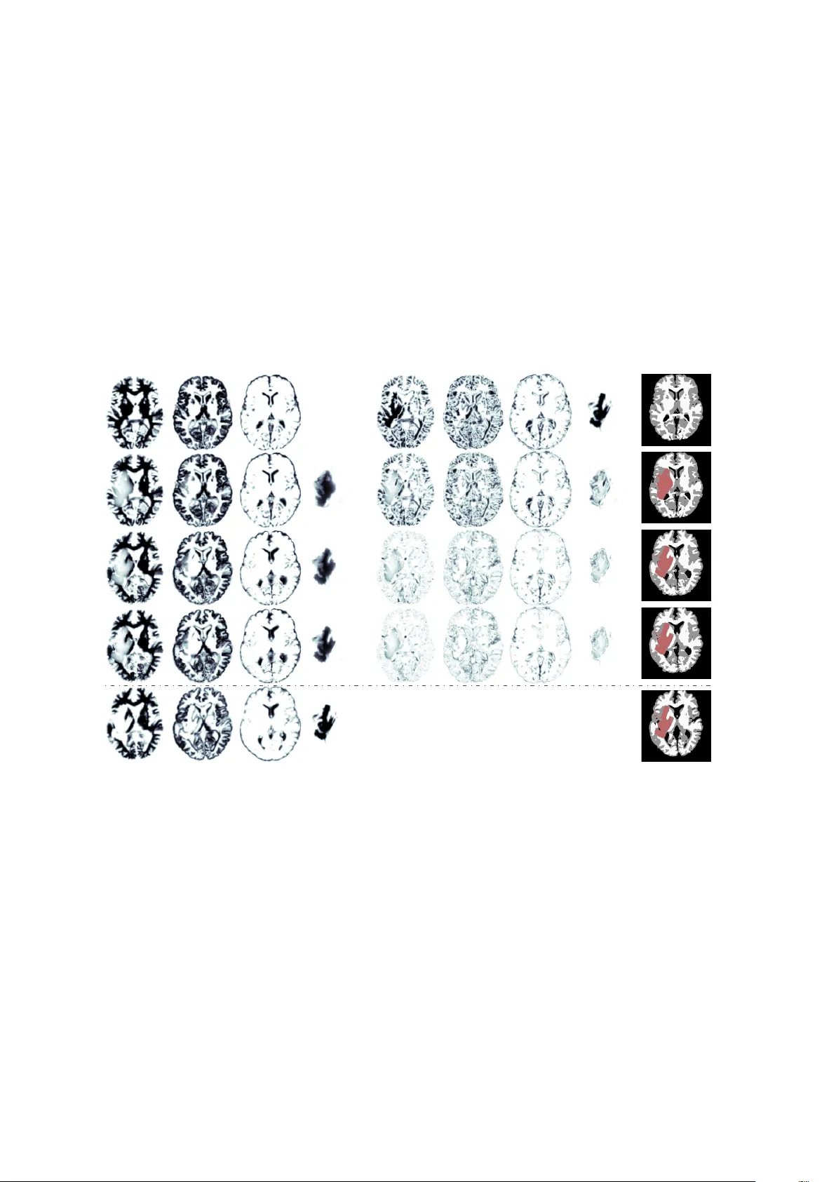
Coupling Brain-T umor Biophysical Models and Dif feomorphic Image Registration Klaudius Scheufele a , Andreas Mang b , Amir Gholami d , Christos Da v atzikos e , George Biros c , Miriam Mehl 1 a a University of Stuttgart, IPVS, Universit ¨ atstraße 38, 70569 Stuttgart, Germany b University of Houston, Department of Mathematics, 3551 Cullen Blvd., Houston, T exas 77204-3008, USA c University of T exas, ICES, 201 East 24th St, Austin, T exas 78712-1229, USA d University of California Berkeley, EECS, Berkeley , CA 94720-1776, USA e Department of Radiology , University of Pennsylvania School of Medicine, 3700 Hamilton Walk, Philadelphia, P A 19104, USA Abstract W e present the SIBIA (S calable Integrated Biophysics-based Image Analysis) framew ork for joint image registration and biophysical inv ersion and w e apply it to analyse MR images of glioblastomas (primar y brain tumors). Giv en the segmentation of a normal brain MRI and the segmentation of a cancer patient MRI, w e wish to deter mine tumor gro wth parameters and a registration map so that if w e “gro w a tu- mor ” (using our tumor model) in the normal segmented image and then register it to the segmented patient image, then the registration mismatch is as small as possible. W e call this “ the coupled problem ” because it tw o-wa y couples the biophysical inv ersion and registration problems. In the image registra- tion step we solv e a large-defor mation dif feomor phic registration problem parameterized by an Eulerian v elocity field. In the biophysical inv ersion step we estimate parameters in a reaction-diffusion tumor gro wth model that is for mulated as a partial differential equation (PDE). In SIBIA, w e couple these tw o steps in an iterativ e manner . W e first presented the components of SIBIA in “Gholami et al, Framework for Scalable Biophysics-based Image Analysis, IEEE/ACM Proceedings of the SC2017” , in which we deriv ed paral- lel distributed memor y algorithms and software modules for the decoupled registration and biophysical inv erse problems. In this paper , our contributions are the introduction of a PDE-constrained optimization formulation of the coupled problem, the derivation of the optimality conditions, and the deriv ation of a Picard iterativ e scheme for the solution of the coupled problem. In addition, w e perfor m sev eral tests to experimentally assess the performance of our method on synthetic and clinical datasets. W e demonstrate the conv ergence of the SIBIA optimization solv er in differ ent usage scenarios. W e demonstrate that us- ing SIBIA, w e can accurately solv e the coupled problem in three dimensions (256 3 resolution) in a few minutes using 11 dual-x86 nodes. Keywords: biophysically constrained diffeomorphic image registration, tumor gro wth, atlas registration, adjoint-based methods, parallel algorithms 2010 MSC: 49K20, 49M15, 35K57, 65K10, 68W10 1. Introduction W e present the SIBIA frame work that comprises a mathematical formulation, algorithms, and softw are for joint image registration and biophysical inv ersio n. Giv en a volumetric segmentation of a magnetic res- onance imaging (MRI) dataset of a glioma (primary brain tumor) patient, SIBIA simultaneously registers 1 Declarations of interest: none Email addresses: klaudius.scheufele@ipvs.uni-stuttgart.de (Klaudius S cheufele), andreas@math.uh.edu (Andreas Mang), amirgh@berkeley.edu (Amir Gholami), christos.davatzikos@uphs.upenn.edu (Christos Da vatzikos), biros@ices.utexas.edu ( George Biros), miriam.mehl@ipvs.uni-stuttgart.de (Miriam Mehl ) Preprint submitted to Computer Methods in Applied Mechanics and Engineering March 5, 2018 A tlas Space P atient Space healthy atlas atlas w/ tumor advected patient patient w/ tumor (a) (b) (c) (d) ? T R Figure 1: Here we summarize the joint r egistration and biophysical inversion in SIBIA. (a) shows the segmented healthy brain (the atlas), (b ) tumor-bearing atlas brain generated by biophysical simulation, (c ) patient tumor register ed to atlas (in atlas space), (d) tumor-bearing patient brain. The inputs are images (a) and (d). The outputs are the tumor growth parameters, the registration parameters, and images (b) and (c). In SIBIA, we compute tumor-growth and registration parameters so that images (b) and (c) are as similar as possible. In this example, the biophysical tumor growth parameters are the initial conditions for a reaction-diffusion equation. The registration is parameterized using an Eulerian framework and a velocity field that is used to advect image (d) to image (c). this image to a segmented MRI dataset of a nor mal brain (an atlas) and fits a biophysical tumor growth model. Such a joint registration-biophysical inv ersion approach is motivated by tw o practical problems: (1) Often, we need to calibrate complex macroscopic biophysical PDE models using a single-time snap- shot dataset. Since the biophysical model is typically a dynamical system, it is unclear how to fit model parameters using just a single-time dataset since w e don’t ha ve the initial state. Replacing the missing second patient snapshot by a healthy atlas and coupling registration between patient and atlas with the tumor gro wth model attempts to resolv e this problem. (2) W e want to register normal MR images to MR images with abnormalities. This nor mal-to-abnormal registration finds applications in surgical planning (e.g., mapping structural and functional infor mation to a patient image), longitudinal studies, followups, or population studies. W e focus on applying SIBIA to the registration of segmented normal images to segmented MR im- ages of glioma patients. Many image analysis workflo ws for gliomas involv e fitting biophysical models for tumor characterization and prognosis ( Sw anson et al. , 2008 ; Rahman et al. , 2017 ), for image registra- tion ( Mohamed et al. , 2006 ; Kw on et al. , 2014a ; Zacharaki et al. , 2009 ), and for image segmentation ( Bakas et al. , 2015 ; Gooy a et al. , 2013 ; Prasta wa et al. , 2009 ). In many methods for these image analysis and biophysical modeling problems, an essential step is the solution of an inv erse tumor-gr o wth problem, i.e., for instance the calculation of the initial conditions for tumor growth; this process can be combined with registration and segmentation as in ( Goo ya et al. , 2013 ). 1.1. Statement of the problem and summary of the approach The specific scenario w e are interested in is summarized in Fig. 1 . W e are giv en a single snapshot of the multi-modal MRI of a glioma patient. Let us assume that w e ha v e obtained a segmentation of the MRI in healthy tissue and abnormal tissue, i.e., w e ha ve labels for white matter , gra y matter , cerebrospinal fluid (CSF), cerebellum, v entricles, and tumor 3 . Since the tumor-gr o wth problem is typically a time dependent problem, w e need at least tw o time snapshots to inv ert for parameters, ideally w e would like to hav e a pre-cancer image of the healthy brain of the patient, the white, gray , and CSF structure, which w e don’t ha ve, though. The basic idea to tackle this issue is to use a pre-segmented nor mal healthy brain (atlas) as a means to create a second snapshot. This is the step that requires registration. The best w a y to describe this is to consider the “forward problem” : Assume w e are giv en the (haelthy) atlas, a tumor-gro wth model, and a defor mation map (represented as adv ection with a giv en velocity field). Then, w e first apply the tumor gro wth model to the healthy image and produce a new segmentation that has both healthy tissue 3 In reality , the tumor has subclasses like edema, necrotic tumor , enhancing tumor , and others. Since w e’re using a very simple tumor model, w e don’t consider these subclases here. 2 and tumor . In a second step, w e w ar p this image using the given defor mation map. This image is the tumor-plus-deformation warped atlas. In the “inverse problem” , w e seek to compute the tumor-gr owth parameters and deformation parameters so that the tumor-plus-deformation warped atlas image matches the patient image. Thus, SIBIA combines the following steps: (i) a for w ard tumor solv er growing a virtual (or synthetic) tumor in the segmented healthy atlas brain, (ii) the inv erse tumor solver determining the initial condition for tumor gro wth giv en an obser v ation at a later time, (iii) a forw ard linear adv ection solver that implicitly computes the w ar ped image giv en the v elocity field, and (iv) a large-deformation diffeomorphic image registration solv er . Both inv ersion and registration are optimization problems. 1.2. Contributions (i) W e for mulate a coupled tumor growth and registration optimization problem in § 3 and deriv e its gradient. (ii) W e deriv e the first order optimality conditions for the joint registration and biophysical inv ersion for brain tumor gro wth. (iii) Instead of using a gradient descent method, w e propose a Picard iteration scheme for solving the system based on modular tumor and image registration components, a generic idea that can be extended to other problems. (iv) W e conduct numerical experiments on synthetic and real data that demonstrate the validity and efficiency of our approach, in particular w e show that the Picard iteration reduces the gradient and conv erges to a local minimum. (v) W e examine the sensitivity of our solv er on the choice of the tumor model v ariant. W e consider three v ariants of the tumor model: a reaction model, a reaction-diffusion model, and a simple radial basis approximation (no time ev olution; the tumor is simply approximated at the obser v ation time). All these v ariants can be used depending on the goal of the analysis. 1.3. Limitations and Open Issues Sev eral limitations and unresolved issues remain. The main limitation is that w e don’t ha ve a theoret- ical proof that the Picard scheme conv erges 4 , w e only pro vide empirical evidence. A second limitation is that our tumor model does not include mass-effect, w e use a simple phenomenological reaction-dif fusion model ( Sw anson et al. , 2000 , 2002 ; Murray , 1989 ). This model, although it has been prov en to be quan- titativ ely useful for image analysis and tumor characterization ( Mang et al. , 2012 ; Swanson et al. , 2008 ; Jackson et al. , 2015 ; Lima et al. , 2016 ), has limited predictiv e capabilities. Its predictiv e capabilities are v er y limited. W e are currently w orking on integrating a mass-effect, which is considered critical for char- acterizing tumor aggressiveness ( Kyriacou et al. , 1999 ; Y ankeelov et al. , 2013 ; Mohamed et al. , 2006 ) as w ell as richer reaction-diffusion models. SIBIA can naturally be extended to these more complex models although of course more tests will be necessary to demonstrate conv ergence of the Picard scheme. 1.4. Literature review W e presented fast algorithms for the individual components of SIBIA in ( Gholami et al. , 2017 ) w ere w e introduced the key computational ker nels (reaction-diffusion, advection, and inverse solution based on FFT and particle-in-mesh methods) and demonstrated their scalability on very large images and distributed-memory architectures. Our problem formulation results in a mixed-type PDE-constrained optimization problem that poses significant numerical challenges. W e refer to ( Biegler et al. , 2003 ; Borz ` ı 4 The optimization problem we’re solving is highly non-convex, so multiple solutions may exist. Our solver conv ergences to a local minimum. 3 and S chulz , 2012 ; Herzog and Kunisch , 2010 ; Hinze et al. , 2009 ) for a general introduction into PDE- constrained optimization and to ( Angelini et al. , 2007 ; Bauer et al. , 2013 ; Mang et al. , 2017 ) for revie ws on its application to medical image analysis. W e will limit ourselves to the w ork most closely related to ours in the follo wing. The first component of SIBIA is image registration. W e refer to ( Modersitzki , 2004 ; S otiras et al. , 2013 ) for a general ov erview of medical image registration. Registering the atlas to the patient requires finding correspondences betw een tw o topologically different images—one with tumor and one without tumor . The key issue here is the ill-defined correspondence arising from the presence of a tumor in only one of the images to be registered. A simple strategy to deal with this issue is to consider the tumor area as non-infor mativ e and mask it from the optimization ( Henn et al. , 2004 ; Stefanescu et al. , 2004 ; Brett et al. , 2001 ) or to relax the registration in the area affected b y the tumor ( Parisot et al. , 2014 ). This, ho w ev er , yields poor registration quality for tumors with sev ere tissue deformation due to mass effect. Another strategy is to simultaneously inv ert for the deformation map and a drift in intensity representing the imaging abnor mality associated with the tumor ( Li , 2010 ; Li et al. , 2012 ), which can also be applied to other registration problems with topological differences (for instance, pre- and postoperativ e image registration ( Kw on et al. , 2014a )). While it may produce acceptable results for the pur pose of atlas-based segmentation and registration, it can not be used in the context of model prediction—which is our ultimate goal. Our prior w ork on diffeomorphic image registration ( Mang and Biros , 2015 , 2016 ; Mang et al. , 2016 ; Mang and Ruthotto , 2017 ; Mang and Biros , 2017 ) forms the basis for the proposed methodology based on the pioneering work in ( Christensen et al. , 1996 ; T rouv ´ e , 1998 ; Beg et al. , 2005 ) (see ( Mang and Biros , 2015 ) for additional references). The second component of SIBIA is the calibration of brain tumor models to medical imaging data ( Gho- lami et al. , 2016b ; Gholami , 2017 ; Gholami et al. , 2017 ; Y ankeelov et al. , 2013 ; Miga et al. , 1998 ). The associated PDE operator is a parabolic, non-linear , reaction-dif fusion equation ( Murray , 1989 ; Swanson et al. , 2002 ). Despite its phenomenological character , this model is capable of generating simulations that are in good agreement with observations of abnor malities in standard MR imaging data and has been used by other groups besides ours ( Clatz et al. , 2005 ; Hogea et al. , 2007 ; Har pold et al. , 2007 ; Konukoglu et al. , 2010b , a ; Le et al. , 2016 ; Lima et al. , 2016 ; Mosa yebi et al. , 2012 ; Menze et al. , 2011 ; Mang et al. , 2012 ; Swanson et al. , 2008 ). Our implementation features inv ersion operators for the initial tumor con- centration, for diffusivity parameters, or for the growth rate ( Gholami et al. , 2016b ). Related optimal control formulations can, e.g., be found in ( Colin et al. , 2014 ; Hogea et al. , 2008b ; Knopof f et al. , 2013 , 2017 ; Liu et al. , 2014 ; Mang et al. , 2012 ; Quiroga et al. , 2015 , 2016 ; W ong et al. , 2015 ). Unlike most existing approaches (with the exception of ( Kwon et al. , 2014b )), our parameterization of the problem ( Gholami et al. , 2016b ; Gholami , 2017 ) allows us to inv ert for multifocal tumors. Numerical methods for solving the tumor calibration problem are based either on point estimate or Ba y esian inference methods ( Lima et al. , 2016 , 2017 ). Bay esian inference characterizes the uncertainty in the model parameters. In this paper , we just focus on methods for point estimates using an adjoint formulation. Our approach can be extended to the Ba yesian setting ( Flath et al. , 2011 ). The integration of biophysical brain tumor simulations with defor mable image registration is not new ( Goo ya et al. , 2013 ; Hogea et al. , 2008a ; Mohamed et al. , 2006 ; Zacharaki et al. , 2008b , a , 2009 ). In ( Mo- hamed et al. , 2006 ; Zacharaki et al. , 2008b , a , 2009 ), a purely mechanical model for tumor progression was used. The tw o key limitations of the work in ( Mohamed et al. , 2006 ; Zacharaki et al. , 2008b , a , 2009 ) are ( i ) that the model is ov ersimplified; it did not provide the capabilities to generate tumors with complex shapes ( ii ) that these models do not pro vide infor mation about the progression and infiltration of cancer- ous cells into surrounding healthy tissue.The proposed formulation does not share these limitations. The w ork that is closest to ours is ( Bakas et al. , 2015 ; Kwon et al. , 2014a ; Hogea et al. , 2008a ; Goo ya et al. , 2013 ). Here, the authors present a framew ork for joint segmentation, registration, and tumor modelling. Like- wise to ours, their approach is based on a PDE constrained optimization problem, where the constraint is a non-linear , mixed-type reaction-diffusion-adv ection equation for the tumor cell density . What sets our w ork apart are ( i ) the solver (w e do not iterate on both control v ariables simultaneously; w e perfor m a block elimination and iterate resulting in an interleav ed optimization on the controls using 4 globalized Newton–Kr ylo v solv ers as opposed to derivativ e free-optimization ( Gooy a et al. , 2013 ; Hogea et al. , 2008a ; Mohamed et al. , 2006 ; Zacharaki et al. , 2008b , a , 2009 ; W ong et al. , 2015 )); ( ii ) an efficient parallel implementation ( Mang et al. , 2016 ; Gholami et al. , 2017 ); ( iii ) the deriv ation of the optimality sys- tems for the fully coupled problem; ( iv ) the parameterization for the initial condition of the tumor , which not only allows us to represent multifocal tumors but also to significantly simplify the PDE constraint without loosing segmentation accuracy; ( v ) and finally the integration with a state-of-the-art algorithm for constrained large defor mation diffeomorphic image registration ( Mang and Biros , 2015 , 2016 ; Mang et al. , 2016 ; Mang and Biros , 2017 ). 1.5. Outline W e present the proposed for mulation for biophysically constrained diffeomorphic image registraiton in § 3 . W e sho w that the optimality systems of our problem are complex, space-time, multi-physics op- erators that pose significant numerical challenges. W e further motivate and explain our choices for the forwar d operators for the tumor model and the registration in § 3.1 and § 3.2 and present the associated in- v ersion operators. In § 4 , w e discuss the algorithmic details. W e summarize the setup for the experiments in § 5.1 and present numerical results on real and synthetic data in § 5 and conclude with § 6 . Additional material is pro vided in § Appendix A . 2. Notation Before presenting the models used for tumor growth and image registration, w e summarize the nota- tion used throughout the manuscript. Segmentation labels and probability maps. For each healthy brain tissue type, i.e., gra y matter (GM), white matter (WM), and cerebrospinal fluid (CSF; which includes the ventricles), w e use a separate probability map. W e represent these probability maps as a space-time v ector field m ( x , t ) = ( m i ( x , t ) ) i = 1,.. .,3 ∈ R 3 with m 1 = m G M , m 2 = m W M , m 3 = m C SF (1) with m i ( x , t ) ∈ [ 0, 1 ] defined on the space-time inter v al Ω × [ 0, 1 ] 3 with boundar y ∂ Ω . The domain occupied by brain tissue (healthy or unhealthy) is denoted by Ω B ⊂ Ω . The fourth probability map is c ( x , t ) ∈ [ 0; 1 ] , also defined in Ω B ; c is the output of the tumor forwar d simulation and represents the probability to encounter cancerous cells at a location x at time t . For conv enience, w e also define the space-time domains U = Ω × ( 0, 1 ] and ¯ U = Ω × [ 0, 1 ) . Labels, i.e., characteristic functions calculated based on giv en threshold values for tumor and healthy tissue types are used only in the ev aluation of our results to compute Dice coefficients. Patient and atlas data. Data of the actual patient image are marked with a subscript T (template, m T , c T ), data of patient images adv ected to the atlas domain with a subscript P ( m P , c P ), and those of the atlas brain with a subscript A ( m A , c A ). Dependency on time and space. In most formulations, w e do not explicitly include the dependency on the spatial position x , but only the time dependency . For instance, c A ( 0 ) denotes the initial tumor probability map defined in the atlas image, whereas c A ( 1 ) is the tumor at time t = 1 (solution of the tumor for w ard problem). This is the point in time associated with the patient image. Probability maps in the atlas image ev olv e in the non-dimensional (tumor gro wth) time inter v al [ 0, 1 ] . For diffeomorphic image registration, w e introduce a pseudo-time variable t ∈ [ 0, 1 ] and inv ert for a stationary v elocity field v ( x ) ; t does not ha ve a physical meaning; w e associate t = 0 with the undeformed patient image (image to be registered; template image) and t = 1 with its defor med representation. W e make more explicit definitions below . 5 V ector notation. Giv en a v ector field m ∈ R 3 , we compute ∇ m = ( ∂ j m i ) i , j = 1,2,3 , ∈ R 3,3 . That is, giv en a v elocity field v ∈ R 3 , ∇ m v ∈ R 3 indicates a matrix-v ector multiplication. The standard scalar product in R 3 is denoted by “ · ” and the outer product betw een tw o v ector fields will be denoted by “ ⊗ ”. In addition, w e define the following inner products: h m , ˜ m i L 2 ( Ω ) 3 B 3 ∑ i = 1 h m i , ˜ m i i L 2 ( Ω ) , k m k 2 L 2 ( Ω ) 3 B 3 ∑ i = 1 k m i k 2 L 2 ( Ω ) . (2) 3. For mulation W e propose a ne w coupled for mulation based on diffeomorphic image registration and inv erse tumor gro wth simulation. As an input, w e take the tumor-free atlas brain geometr y m A ( x , 0 ) (reference image, healthy atlas) and the tumor-bearing patient geometry m T ( x ) (template image, patient with tumor) plus the patient’s tumor probability map c T ( x ) (template tumor). Our formulation is based on optimal control theory and results in a coupled PDE-constrained optimization problem. W e inv ert for a stationary v elocity field v ( x ) : = ( v 1 ( x ) , v 2 ( x ) , v 3 ( x ) ) T (establishes the spatial correspondence betw een the patient and atlas image), a parameter vector p (parametrizes the simulated tumor in the tumor-fr ee atlas image), and a mass-source map w ( x ) (controls the computed deformation patter n) as follows: min v , p , w J ( v , p , w ) with J ( v , p , w ) : = D c ( c A , c P ) + D m ( m A , m P ) + β p S p + β v S v + β w S w (3a) subject to ∂ t c A − div k ∇ c A − f ( c A ) = 0 in U , (3b) c A ( 0 ) = Φ p in Ω , (3c) ∂ t m P + ∇ m P v = 0 in U , (3d) m P ( 0 ) = m T in Ω , (3e) ∂ t c P + ∇ c P · v = 0 in U , (3f) c P ( 0 ) = c T in Ω , (3g) div v = w in U (3h) m A ( 1 ) = m A ( 0 ) ( 1 − c A ( 1 ) ) in Ω (3i) with periodic boundar y conditions on ∂ Ω . The objectiv e functional J in ( 3b ) consists of the following building blocks: (i) the tw o driving L 2 -distance measures D c ( c A , c P ) : = 1 2 k c A ( 1 ) − c P ( 1 ) k 2 L 2 ( Ω ) , and D m ( m A , m P ) : = 1 2 k m A ( 1 ) − m P ( 1 ) k 2 L 2 ( Ω ) 3 that measure the discrepancy betw een the simulated tumor in atlas space c A ( 1 ) (solution of the tumor for w ard problem ( 3b ) with initial condition ( 3c ) parametrized b y p ) and the transported probability map c P ( 1 ) of cancerous cells for the patient data (solution of the registration forw ard problem ( 3f ) with initial condition ( 3g )) and the discrepancy betw een the healthy tissue probability maps in atlas space with tumor (calculated according to ( 3i )) and the transported probability maps of healthy tissue for the patient data (solution of the registration for w ard problem ( 3d ) with initial condition ( 3e )); (ii) three regularization operators balanced against the discrepancy measures D c and D m based on reg- ularization w eights β j > 0, j ∈ { v , w , p } inv olving 6 (a) a regularization operator S p for Φ p (an L 2 -norm; defined in ( 7 ) in § 3.1 ), (b) a regularization operator S v for v (an H 1 Sobolev norm; defined in ( 13b ) in § 3.2 ), and (c) a regularization operator S w for w (an H 1 Sobolev norm; defined in ( 13b ) in § 3.2 ). The remaining parameters are defined as follo ws: k : Ω B → R 3 × 3 is a diffusion tensor field parametri- zed by scalar w eights that specify the diffusivity in WM and GM (see ( Gholami et al. , 2016b ) for details) and ρ > 0 is the growth parameter for the logistic growth function f ( c A ) : = ρ c A ( 1 − c A ) in ( 3b ). Both k and ρ ha ve different values in gra y matter and white matter and vanish ev er ywhere else. Although our implementation is general, in all our experiments k is just an isotropic diagonal tensor (a scalar function times the identity tensor). The image registration v elocity v is used to transport both the brain geometr y m T and the tumor concentration c T from patient to atlas space. ( 3i ) defines the model for the effect of tumor gro wth on the brain geometry m A ( 0 ) in the atlas space. W e solv e this coupled inv erse problem with gradient-based optimization. W e use the method of Lagrange multipliers to transfor m the constrained problem ( 3 ) into an unconstrained one. The Lagrangian of ( 3 ) reads L G ( c A , c P , m P , m A ( 1 ) , α , λ c , λ m , ν , ξ , p , v , w ) = J ( p , v , w ) + h α ( 0 ) , ( c A ( 0 ) − Φ p ) i L 2 ( Ω ) + Z 1 0 h α , ∂ t c A − ∇ · ( k ∇ c A ) − f ( c A ) i L 2 ( Ω ) d t + Z 1 0 h λ m , ∂ t m P + ∇ m P v i L 2 ( Ω ) 3 d t + h λ m ( 0 ) , m P ( 0 ) − m T i L 2 ( Ω ) 3 + Z 1 0 h λ c , ∂ t c P + ∇ c P · v i L 2 ( Ω ) d t + h λ c ( 0 ) , c P ( 0 ) − c T i L 2 ( Ω ) + Z 1 0 h ν , div v − w i L 2 ( Ω ) d t + h ξ , m A ( 1 ) − ( 1 − c A ( 1 ) ) m A ( 0 ) i L 2 ( Ω ) 3 , (4) with the state fields c A , c P , m P , and m A ( 1 ) , the adjoint fields α , λ c , λ m , ν , and ξ , and the inv ersion fields p , v , and w . The strong for m of the first-order optimality conditions for Equation 4 is given b y the follo wing equations: tumor forward δ α L G = 0 : giv en by ( 3b ) and ( 3c ) (5a) tumor adjoint δ c A L G = 0 : − ∂ t α − ∇ · k ∇ α − α ρ + 2 α ρ c A = 0 in ¯ U , (5b) δ c A ( 1 ) L T = 0 : c P ( 1 ) − c A ( 1 ) − ξ m A ( 0 ) − α ( 1 ) = 0 in Ω . (5c) registration forward δ λ L G = 0 : giv en by ( 3d ) – ( 3h ) (5d) registration adjoint δ m P L G = 0 : − ∂ t λ m − div ( λ m ⊗ v ) = 0 in ¯ U , (5e) δ m P ( 1 ) L G = 0 : m A ( 1 ) − m P ( 1 ) − λ m ( 1 ) = 0 in Ω , (5f) δ c P L G = 0 : − ∂ t λ c − div ( λ c v ) = 0 in ¯ U , (5g) δ c P ( 1 ) L G = 0 : c A ( 1 ) − c P ( 1 ) − λ c ( 1 ) = 0 in Ω , (5h) adjoint coupling δ m A ( 1 ) L G = 0 : m P ( 1 ) − m A ( 1 ) − ξ = 0 in Ω . (5i) tumor inversion δ p L G = 0 : ∇ p S p ( p ) − Φ T α ( 0 ) = 0 in Ω . (5j) registration inversion δ v L G = 0 : ∇ v S v ( v ) + K [ Z 1 0 ( ∇ m P ) T λ m + ∇ c P λ c d t ] = 0 . (5k) Note, that ( ∇ m ) T λ = ∑ 3 i λ i ( ∂ 1 m i , ∂ 2 m i , ∂ 3 m i ) T and that we ha v en’t giv en an equation for w . The operator K in ( 5k ) is a pseudo-differential operator that is deriv ed b y eliminating w in ( 3h ). W e discuss it further in § 3.2 . In summar y , the first-or der optimality conditions ( 5 ) comprise a system of non-linear partial differential equations, which is quite for midable since it has 11 fields in addition to the tumor initial 7 condition parameters p . Given m T , c T , m A ( 0 ) , and k and ρ (in that atlas space at t = 0), w e need to solve the first-order optimality PDEs for the state, adjoint, and inv ersion v ariables. W e use an elimination method (or also called a “reduced-space method” ( Nocedal and W right , 2006 ; Borz ` ı and S chulz , 2012 )) to solve these equations. That is, we assume that the state and adjoint equations are fulfilled exactly and require vanishing v ariations of the Lagrangian with respect to the inv ersion variables v , w , and p for an admissible solution of our problem. In our algorithm, we iterate only on p and v as w e eliminate w . Giv en p and v , w e wish to compute the gradient of J , i.e., g p and g v used to update p and v , respectiv ely . The gradient computation inv olv es the following steps: 1. Solve the forwar d tumor gro wth and registration equations ( 3c )–( 3i ) for the state v ariables c A ( t ) , c P ( t ) , m P ( t ) , m A ( 1 ) . 2. Compute the coupling adjoint v ariable ξ from equation ( 5i ). 3. Solve the adjoint tumor equations ( 5b ) and ( 5c ) for α ( t ) . 4. Solve the adjoint registration equations ( 5e )–( 5h ) for λ m ( t ) and λ c ( t ) . 5. Ev aluate the gradients using the inversion equations ( 5j ) and ( 5k ) at v and p : g v = β v ∇ v S v ( v ) + K [ Z 1 0 ( ∇ m P ) T λ m + ∇ c P λ c d t ] , g p = β p ∇ p S p ( p ) − Φ T α ( 0 ) . (6) At a stationary point g = ( g v , g p ) T v anishes. In § 3.1 and § 3.2 , w e present more details for the tumor forwar d problem ( 3b ), ( 3c ) and the registration forwar d problems ( 3d ), ( 3f ), ( 3e ), ( 3g ), respectiv ely . In addition, w e for mulate separate inv erse problems for tumor gro wth and image registration that are used as high-lev el components in our coupling algorithm presented in 4.1 . The latter is based on a Picard iteration using tumor and registration as modular components instead of a gradient descent or Newton method with line search for the coupled problem ( 3 ). 3.1. The T umor Model Forward T umor Problem. W e model the tumor growth based on the population density c A ( x , t ) . T w o main phenomena are included: proliferation of cancerous cells and the net migration of cancer- ous cells into surrounding healthy tissue ( Murra y , 1989 ) 5 . The proliferation model is a logistic gro wth function f ( c A ) : = ρ c A ( 1 − c A ) with reaction coefficient ρ ( x ) : = ρ f ρ 0 ( x ) . ρ f denotes the scaling of the spatially variable characteristic gro wth rate parameters defined b y white and gray matter , i.e., ρ 0 ( x ) : = ρ w m W M ( x ) + ρ g m G M ( x ) . The migration model is based on an inhomogeneous (potentially anisotropic) diffusion process with diffusion coefficient k ( x ) : = k f k 0 ( x ) I + k a T ( x ) . Here, k f and k a are the scaling factors for the isotropic and anisotropic parts of the diffusion tensor , T ( x ) is a w eighted diffusion tensor modelling anisotrop y . In our test cases in § 5 , we alw a ys use isotropic diffusion, i.e., k a = 0. The isotropic part is k 0 ( x ) : = k w m W M ( x ) + k g m G M ( x ) . This yields a non-linear parabolic PDE with non-constant coeffi- cients for the tumor concentration c given by ∂ t c A − div k ∇ c A − f ( c A ) = 0 in Ω B × ( 0, 1 ] , (7a) ∂ n c A = 0 on ∂ Ω B × ( 0, 1 ] , (7b) c A ( 0 ) = Φ p in Ω B . (7c) W e use a parametrization Φ p for the tumor initial condition c A ( 0 ) as originally in ( 7c ) in an n p -dimensional space spanned b y a Gaussian basis functions, i.e., p ∈ R n p , Φ p : = ∑ n p i = 1 Φ i p i with Gaussian basis functions Φ i : Ω B → R . W e set the Gaussians in CSF to zero to prev ent a spurious diffusion of cancerous cells into the area associated with CSF . 5 Displacement of healthy tissue as a result of tumor growth (mass effect) is currently neglected in our model. 8 For notational conv enience, w e represent the process of solving ( 7 ) with the operator T fw d ( p ) : = c A ( 1 ) (8) mapping the parametrization p of the initial conditions in ( 7c ) to the tumor density c A ( 1 ) at time t = 1. This simple model is b y no means predictiv e on its o wn, but is the de-facto standard approach when it comes to modeling tumor progression as seen in medical imaging ( Sw anson et al. , 2000 , 2008 ; Clatz et al. , 2005 ; Har pold et al. , 2007 ; Konukoglu et al. , 2010b ; Hogea et al. , 2008a ). S ome results av ailable in the literature ha ve suggested that this model can offer (to some extent) predictiv e capabilities when integrated with medical imaging infor mation ( Swanson et al. , 2000 ; T omer et al. , 2014 ). Its usefulness is in segmentation and registration algorithms that use normal atlas information and in producing features (e.g., tumor parameters) to augment image-based features for tumor staging and prognosis. Note that un- like § 3 , w e ha ve stated the tumor problem in Ω B with Neumann boundary conditions ( 7b ), which is the actual biophysical problem. In our numerical implementation, ho w ev er , w e extend k by a small parame- ter , set ρ = 0 in Ω \ Ω B , discretize in Ω using periodic boundar y conditions and use a penalty approach to approximate the boundary conditions at ∂ Ω B . One can sho w that this ‘’fictitious domain method‘’ approximates ( 7 ) and as w e refine the discretization it conv erges to the correct solution (compare ( Hogea et al. , 2008a ; Gholami et al. , 2016b )). Inverse T umor Problem. In the inv erse tumor problem, we seek an initial condition for the forwar d tumor problem that reco v ers a given tumor concentration c P ( 1 ) at time t = 1 as good as possible, i.e., w e solv e the minimization problem min p J T ( p ) with J T ( p ) : = D c ( c A , c P ) + β p 2 k Φ p k 2 2 (9a) subject to the constraints ( 7a ), ( 7b ), and ( 7c ). This defines the inv erse tumor operator T inv ( c P ( 1 ) ) : = p = arg min q J T ( q ) . (9b) Note that the inv erse tumor problem does — in contrast to ( 3b ) — only minimize the mismatch betw een the obser v ed and the predicted tumor cell population density; the healthy tissue mismatch is not used as the tumor solv er only ’knows’ the altas. In addition, ( 9 ) defines a concrete instance for the tumor regularization operator S p in ( 3 ). Neglecting the boundar y conditions, the Lagrangian of ( 9 ) reads L T ( c A , p , α ) = J T ( p ) + h α ( 0 ) , c A ( 0 ) − Φ p i L 2 ( Ω B ) + Z 1 0 h α , ∂ t c A − ∇ · k ∇ c A − ρ c A ( 1 − c A ) i L 2 ( Ω B ) d t W e require v anishing variations of the Lagrangian L T with respect to the inv ersion v ariable p for an admissible solution to ( 9 ). This yields the first order optimality condition of the tumor problem: tumor forward δ α L T = 0 : giv en b y ( 7 ) (10a) tumor adjoint δ c A L T = 0 : − ∂ t α − ∇ · k ∇ α − α ρ + 2 α ρ c A = 0 in Ω B × [ 0, 1 ) (10b) δ c A ( 1 ) L T = 0 : c P ( 1 ) − c A ( 1 ) − α ( 1 ) = 0 in Ω B , (10c) tumor inversion δ p L T = 0 : β p Φ T Φ p − Φ T α ( 0 ) = 0 in Ω B , . (10d) Similarly to the for w ard problem, the adjoint equation are discretized b y extending k and setting ρ = 0 in Ω \ Ω B and using periodic boundary conditions in ∂ Ω . 3.2. The Registration Problem The input for our for mulation are not image intensities ( Mang and Biros , 2015 , 2016 ; Mang and Ruthotto , 2017 ; Mang and Biros , 2017 ) but the probability maps for tissue classes (see ( 1 ); WM, GM, CSF , 9 and tumor). The formulation w e propose here is suited for general problems that involv e the registration of vector fields. The template image (image to be register ed) m T : ¯ Ω → R 3 is given by the probability maps of the patient’s healthy anatomy in all areas except the part hidden by the tumor . W e treat the probability map for the tumor , c T ( x ) , as an individual entity to make the coupled formulation in ( 3 ) more accessible. W e register the three probability maps for healthy tissue and the tumor concentrations. Advective Image T ransformation (Forward Problem). Giv en some template image m T ( x ) , some tu- mor concentration c T ( x ) , and a stationary velocity field v ( x ) , the for w ard problem describes the adv ective transformation of m T and c T in a pseudo-time interval [ 0, 1 ] : ∂ t m P + ∇ m P v = 0 in Ω × ( 0, 1 ] , (11a) m P ( 0 ) = m T in Ω , (11b) ∂ t c P + ∇ c P · v = 0 in Ω × ( 0, 1 ] , (11c) c P ( 0 ) = c T in Ω (11d) with periodic boundar y conditions. W e augment this formulation by an additional constraint on the div ergence of v to better control the Jacobian of the computed deformation map (see ( Mang and Biros , 2016 ) for additional details): div v = w in Ω , (11e) Solving ( 11 ) defines the implicitly given operator R fw d ( v , m T , c T ) : = ( m P ( 1 ) , c P ( 1 ) ) (12) that maps the template images m T and c T to images m P and c P defined at pseudo-time t = 1. For sim- plicity , we will later slightly abuse our notation and use the operator R fw d also for the adv ection of only m , c or one of the components of m , i.e., m W M , m G M , or m C SF . Image Registration (Inverse Problem). In the inv erse problem, i.e., the actual image registration, w e look for a v elocity v that adv ects the giv en template (patient) images to images that are as close as possible to the corresponding images in the atlas brain (denoted with a subscript A ). That is, w e solv e the follo wing minimization problem: min v J R ( v ) with J R ( v ) : = D m ( m A , m P ) + D c ( c A , c P ) + β v S v ( v ) + β w S w ( w ) (13a) subject to ( 11 ). The regularization in ( 13a ) is a smoother for v and w and given b y an H 1 -seminorm for v , and an H 1 -norm for w (i.e., for div v according to ( 11e )), respectiv ely: S v ( v ) = 1 2 Z Ω 3 ∑ i = 1 |∇ v i ( x ) | 2 d Ω , S w ( w ) = 1 2 Z Ω |∇ w ( x ) | 2 + | w | 2 d Ω . (13b) Ov erall, this defines the (inv erse) image registration operator R inv ( m A ( 1 ) , c A ( 1 ) , m T , c T ) : = v = arg min u J R ( u ) . (13c) The Lagrangian for our image registration problem reads L R ( c P , m P , v , λ m , λ c ) = J R ( v ) + Z 1 0 h λ m , ∂ t m P + ∇ m P v i L 2 ( Ω ) 3 d t + h λ m ( 0 ) , m P ( 0 ) − m T i L 2 ( Ω ) 3 + Z 1 0 h λ c , ∂ t c P + ∇ c P · v i L 2 ( Ω ) d t + h λ c ( 0 ) , c P ( 0 ) − c T i L 2 ( Ω ) + Z 1 0 h ν , div v − w i L 2 ( Ω ) d t . 10 T aking v ariations, w e obtain the first-order optimality conditions ( Mang and Biros , 2016 ) for the registra- tion problem: registration forward δ λ m , λ c L R = 0 : giv en by ( 11 ) (14a) registration adjoint δ m P L R = 0 : − ∂ t λ m − div ( λ m ⊗ v ) = 0 in U , (14b) δ m P ( 1 ) L R = 0 : m A ( 1 ) − m P ( 1 ) − λ m ( 1 ) = 0 in Ω , (14c) δ c P L R = 0 : − ∂ t λ c − div ( λ c v ) = 0 in U , (14d) δ c P ( 1 ) L R = 0 : c A ( 1 ) − c P ( 1 ) − λ c ( 1 ) = 0 in Ω , (14e) registration inversion δ v L R = 0 : β v ∇ v + K [ Z 1 0 ( ∇ m P ) T λ m + ∇ c P λ c d t ] = 0 in Ω . (14f) As mentioned before, the operator K is a pseudo-differential operator and comes from an elimination step for the inv ersion v ariable w in ( 3h ). For the case of exact incompressibility ( w = 0), it is the Leray projection K ( u ) : = u + ∇ ∇ − 1 div u ; for a non-zero w , the projection operator becomes slightly more inv olv ed; w e refer to ( Mang and Biros , 2015 , 2016 ) for additional details. 4. Numerical Methods The main contribution of this paper is a Picard iteration scheme for ( 3 ): Instead of solving ( 3 ) using a gradient descent or Newton scheme, w e use a modular approach, in which w e combine tumor gro wth inv ersion and diffeomorphic registration models in an (interlea v ed) Picard iteration scheme. This scheme iterativ ely impro ves both the tumor initial condition’s parametrization p and the registration v elocity v . This allows us to establish a coupling of both components in an easy , stable, modular , and efficient wa y; the submodules can be exchanged as required. For instance, our simple tumor solv er can be replaced b y more sophisticated approaches. Our results presented in § 5 demonstrate that the Picard iteration is a po w erful approach that reduces the gradient as giv en in ( 6 ). The algorithms for the individual subblocks ha ve been published in ( Mang and Biros , 2015 , 2016 ; Gho- lami et al. , 2017 , 2016b , a ; Mang et al. , 2016 ; Mang and Biros , 2017 ). The main ingredients can be described as follows: (i) All PDEs are spatially discretized in Ω = [ 0, 2 π ] 3 . (ii) All spatial derivativ es ( ∇ , div , and higher deriv ativ es) are computed using 3D Fourier transfor ms. (iii) Although in the formulation w e present the deriv atives in the strong for m, in our implementation w e use a discretize-then-optimize approach for the tumor equations and an optimize-then-discretize approach for the registration. (iv) The solution of pure adv ection equations is done using a semi-Lagrangian time-stepping scheme to av oid stability issues and small time-steps. (v) W e use Kr ylo v and matrix-free Newton methods for linear and nonlinear solv ers. (vi) W e use a Picard iteration scheme for the coupled optimization problem, without line search 6 . In the follo wing subsections, w e giv e more details on the proposed Picard iteration scheme, and then giv e a short ov er vie w of the numerical methods used to solv e the tumor and image registration for w ard and inv erse problems. 4.1. The Picard Iteration Algorithm T o initialize our Picard iteration, w e start with an initial guess for p ∈ R n p and v (both zero), compute the center of mass of the giv en patient tumor c T and place the Gaussian basis functions for the tumor initial condition parametrization as a regular grid around the center of mass. In our current algorithm, the grid of Gaussian basis functions is fixed throughout the Picard iterations, i.e., w e do not re-compute the center of mass of the tumor or adv ect the Gaussian basis functions with the v elocity v (this is ongoing w ork). The algorithm per Picard iteration executes the following steps: 6 The Newton-type iterations for the sub-problems registration and tumor inv ersion are enhanced with a globalizing line search method. 11 1. Giv en some p , gro w a tumor in the atlas space. This seeds the atlas brain with a tumor; update the probability maps at t = 1 in the atlas space using ( 3i ). T o define the Picard iteration, it is useful to introduce the operator G G ( c A ( 1 ) ) : = ( m A ( 0 ) ( 1 − c A ( 1 ) ) , c A ( 1 ) ) . (15) 2. Register the probability maps (for the anatomical regions and the tumor) given for the patient’s image with the updated probability maps in the atlas space. 3. Use the computed v elocity v to transport the patient data (probability maps for the anatomical regions and the tumor) to the reference atlas space. This giv es us a new m P ( 1 ) and c P ( 1 ) . 4. Use the transported (i.e., updated) c P ( 1 ) within the tumor inv ersion to find a better p . 5. Check for conv ergence. If the conv ergence criteria are fulfilled, stop. If not, go back to step 1 (i.e., continue iterating). Some important facts to note are: (i) W e use the solution v from the former iteration as an initial guess for the next iteration to reduce the runtime (w arm start). (ii) W e perform a continuation in the regularization parameter β v (w e start with a large v alue and successively reduce it). W e explain this belo w . (iii) W e do not ha v e a proof for the conv ergence of the proposed Picard scheme to a minimizer of the fully-coupled optimization problem in ( 3 ). Such a proof is bey ond the scope of the present paper and remains for future w ork. W e pro vide numerical evidence that sho ws that our scheme reduces the gradient of the fully-coupled problem. W e discuss this below . Using the operators defined in § 3 , the described algorithm corresponds to the Picard iteration p k + 1 = T inv ◦ R fw d  R inv  G ◦ T fw d ( p k ) , m T , c T  , c T  for the parametrization p of the tumor initial conditions c A ( 0 ) in the atlas brain with probability maps m T and c T for an individual patient as input (w e use R fw d here to only adv ect the patient’s tumor c T ). W e hav e implemented the gradient of the coupled problem in § 3 in order to v erify that our Picard it- eration actually reduces the gradient of the global optimization problem. An implementation of a scheme that iterates simultaneously on both control v ariables (i.e., solv es the global problem), requires more w ork and will be addressed in a follow-up paper . W e show experimentally in v arious settings that our algo- rithm is effectiv e and generates registration results that are in excellent agreement with the patient data. Next, w e giv e additional details on the numerical methods used in SIBIA. Parameter continuation. W e use a combination of T ikhonov-type regularization and parameter con- tinuation (additional details can be found in ( Mang and Biros , 2015 )) not only to stabilize the registration problem, but also to identify an adequate regularization parameter β v for the H 1 -Sobolev nor m for v in ev ery Picard iteration as follows. W e specify a low er admissible bound on the determinant of the defor- mation gradient and start the Picard iteration with β 0 v = 1. In each iteration k , the candidate β k v is reduced b y one order of magnitude until the specified low er bound for the deter minant of the deformation gra- dient is breached for a candidate β k v . The registration solv er disregards the associated solution, sets the candidate value for β k v to β k v ← β k − 1 v − ( β k − 1 v − β k v ) / 2 and restarts the inversion with the v elocity of the former Picard iteration as initial guess. This process is repeated until the lo wer bound for the determinant of the deformation gradient is no longer violated. If no violation of the deter minant of the deformation gradient was detected during the registration solve, we finalize the current Picard iteration and proceed with the next iteration. Stopping conditions. W e finalize our Picard iteration either if β v reaches the prescribed minimum 7 or if the requested β v results in a violation of a user defined lo w er bound on the determinant of the defor- 7 This low er bound is chosen based on numerical experience and is a safeguard against numerical instabilities that can occur if v becomes highly irregular (see ( Mang and Biros , 2017 ) for a discussion). 12 mation gradient (see abo v e for further explanation). In both cases, w e execute tw o additional iterations with the final v alue for β v . 4.2. Numerics for the tumor inversion and registration sub-blocks The optimality conditions of both ( 9a ) and ( 13a ) are complex, multi-component, non-linear opera- tors for the state, adjoint, and control fields. W e emplo y an inexact, globalized, preconditioned Gauss– Newton–Krylov method for both problems. In reduced space methods, the second order optimality conditions ha v e a v er y similar structure as the first order optimality conditions; we can employ the same numerical strategies w e use for the solution of the PDE operators in the first order optimality conditions (see below). W e refer to ( Gholami et al. , 2016b ; Mang and Biros , 2015 , 2017 ; Mang et al. , 2017 ) for details on the reduced space Hessian system and its discretization. Numerical solution and discretization of the PDE operators. T o discretize forwar d and adjoint tumor and registration pr oblems in space and time, w e use regular grids consisting of N 0 × N 1 × N 2 , N i ∈ N grid points. For all spatial differ ential operators, w e use a spectral projection scheme as described in ( Gholami et al. , 2017 ; Mang et al. , 2016 ). The mapping betw een the spatial and spectral coefficients is done using FFT s (the implementation of the parallel FFT library is presented in ( Gholami et al. , 2016a )). Correspond- ing to the spectral collocation scheme, w e assume that the functions in our formulation (including images) are periodic and continuously differentiable and apply filtering operations and periodically extensions of the discrete data to meet these requirements. T o solv e the for w ard and adjoint tumor problem, we use an unconditionally stable, second-order Strang-splitting method, where w e split the right-hand side of ( 7a ) and ( 10b ) into diffusion and reaction (see ( Hogea et al. , 2008a ; Gholami et al. , 2016b ) for details). The diffusion sub-steps are solv ed using an implicit Crank–Nicolson method. The solv er is a preconditioned conjugate gradient method with a fixed tolerance of 1E − 6. The reaction sub-steps are solv ed analytically . W e enforce a positivity constraint on the initial tumor concentration before w e apply the forwar d operator to make sure that c ( x , t ) is in [ 0, 1 ] for all x ∈ Ω and t ∈ [ 0, 1 ] . This thresholding operation is necessar y since the parametrization allows for negativ e concentrations for the initial condition c A ( 0 ) (the coefficient v ector p can ha v e negativ e entries) and the logistic gro wth function would amplify these negative values in time. In the image registration module, w e solve the hyperbolic transport equations in ( 11 ) based on a semi-Lagrangian scheme ( Mang et al. , 2016 ; Mang and Biros , 2017 ). S emi-Lagrangian schemes are a hy- brid betw een Lagrangian and Eulerian schemes. They are unconditionally stable and, like Lagrangian schemes (see ( Mang and Ruthotto , 2017 ) for an example in the context of dif feomorphic registration), require the ev aluation of the space-time fields that appear in our optimality conditions at off-grid loca- tions defined by the characteristic associated with v . W e compute the values of these space-time fields at the off-grid locations with a cubic Lagrange polynomial interpolation model. The time integration for computing the characteristic and for the solution of ordinary differential equations along it (if necessar y) is based on a second order accurate Runge–Kutta scheme. W e refer to ( Mang et al. , 2016 ; Mang and Biros , 2017 ) for a precise definition of these computations. Newton–Krylov solver . W e initialize our solv ers for both reduced gradient systems ( 10d ) and ( 14f ) with a zero initial guess and use an inexact, globalized, preconditioned Gauss–Newton–Krylov method. W e terminate the tumor inversion if the relativ e change of the nor m of the reduced gradient in ( 10d ) is belo w a user defined threshold opttol T > 0. The reference gradient is the gradient obtained for the zero initial guess for p in the first Picard iteration. For the registration problem, we use a combination of the relativ e change of ( i ) the norm of the gradient in ( 14f ), ( ii ) the objectiv e in ( 13a ) and ( iii ) the control v ariable v , all controlled b y a single parameter opttol R > 0, as a stopping criterion. W e also specify a maximal number of Newton iterations (maxit N , T and maxit N , R ) and a low er bound of 1E − 6 for the absolute nor m of the gradient as a safeguard against a prohibitiv ely high number of iterations. Details for the stopping conditions can be found in ( Mang and Biros , 2015 ; Modersitzki , 2009 ); see ( Gill et al. , 1981 , 305 ff.) for a discussion. 13 W e inv ert the inner linear KKT systems using a matrix-free PCG method. W e ter minate the PCG method when w e either reach a predefined tolerance for the relativ e residual norm of the PCG method or exceed the maximum number of iterations (maxit K , T and maxit K , R ). W e perfor m inexact solv es ( Dembo and Steihaug , 1983 ; Eisentat and W alker , 1996 ) with a tolerance that is proportional to the nor m of the reduced gradient of our problem. The key idea here is to not inv ert the Hessian accurately if w e are far from an optimum (large gradient norm). Details about this approach can be found in ( Nocedal and W right , 2006 , p. 165ff.). 4.3. Parallel Algorithms and Computational Kernels Our parallel implementation is described in detail in ( Mang et al. , 2016 ; Gholami et al. , 2017 ). W e use a 2D pencil decomposition for 3D FFT s ( Grama et al. , 2003 ; Czechowski et al. , 2012 ) to distribute the data among processors. W e denote the number of MPI tasks b y P = P 0 P 1 . Each MPI task gets a total of N 0 / P 0 × N 1 / P 1 × N 2 v alues. W e use the open source library AccFFT ( Gholami et al. , 2016a ), which supports parallel FFT on CPU and GPU for both single and double precision computations. For parallel linear algebra operations, we use PETSC as w ell as it’s optimization interface T AO ( Bala y et al. , 2016 ; Munson et al. , 2015 ). The other computational kernel besides FFT s is the cubic Lagrange polynomial interpolation model used for the semi-Lagrangian time integration of hyperbolic transport equations. W e refer to ( Mang and Biros , 2016 ; Gholami et al. , 2017 ) for additional details on the parallel implementation of this interpolation kernel. W e provide an algorithmic complexity analysis for the registration in ( Mang et al. , 2016 ) and for the FFT in ( Gholami et al. , 2016b ). 5. Numerical Exper iments W e test the performance of our method on synthetically generated and clinical datasets. Both are based on real MR neuroimaging data for the brain tissue probability maps. A T A V . This first class of synthetic test cases is used as a proof of concept to assess the conv ergence of our Picard scheme, its robustness with respect to the tumor model, and the sensitivity of tumor re- construction quality in ter ms of the tumor model and its parameters. It uses analytic tumor and analytic v elocity (fully synthetic; ground truth for tumor parameters and v elocity is known); see § 5.2 for details. It comes in three differ ent flav ours: ( i ) A T A V -REAC with reaction only and dif fusion disabled, ( ii ) A T A V -DIF with reaction-duffusion model, and ( iii ) A T A V-LD with reaction only and diffusion disabled and a small number n p of Gaussian basis functions for the initial condition. 8 R TR V . This second second class of test cases uses real clinical images used in the study described in ( Goo ya et al. , 2013 ). It uses real patient data, diffusion disabled and enabled; see § 5.3 for details. 5.1. General Setup Common Parameters. W e list all model and numerical par meters that are common to all test cases in T ab. 1 and those that are specific for the test cases in T ab. 2 . In the follo wing, we shortly motivate some of the more inv olv ed choices: β p has been determined experimentally for a purely synthetic test case with image resolution N i = 128 and n p = 125 Gaussian basis function. For variations of N i and n p in our test cases, w e observed that the inv ersion is not sensitiv e with respect to β p . Accordingly , w e fixed it for all test cases. Smaller values did not further reduce the tumor mismatch in our Picard iteration scheme. T o initialize the Gaussian basis, the sub-domain for the grid of basis functions is chosen a priori for the synthetic test cases and determined automatically for the real patient data (cases RTR V) to cov er the actual tumor v olume in an optimal w a y: W e set the center of the grid for the parameterization to the center of mass of the tumor . The 8 LD stands for low-dimensional. That is, w e use only very few activ e Gaussian basis functions with a limited support in a small neighbourhood surrounding the center of mass of the patient’s tumor . For the other test cases, w e allow the grid for the Gaussian to cov er the entire area identified as tumor in the patient data. 14 support of the domain cov ered by the basis functions is the ` ∞ -ball that cov ers the entire patient’s tumor in R 3 . W e adjust the standard deviation σ of the Gaussian functions and the distance of their centers automatically . The v alues are chosen such that their quotient remains constant, and equal to the v alue used in the synthetic cases. This allows us to ensure a similar conditioning for Φ and to use a fixed β p . The choice for n p depends on the appearance of the patient’s tumor (shape and size). W e need to be able to parameterize sufficiently complex initial conditions to reco v er tumors with a complex appearance. Accordingly , w e inv ert for a varying number of parameters n p on a case-by-case basis ( n p ∈ { 8, 125, 343 } (see T ab. 2 ). For the class of synthetic test cases (A T A V), w e use an image resolution of 128 3 to be able to perform more experiments in limited time, for the real patient data, w e use 256 3 to ensure high accuracy . T able 1: Common parameters used in all test cases: opttol R , opttol T are the convergence tolerances for registratioin and tumor inversion ( ( 14f ) and ( 10d ) ); β p is the regularization parameter for the tumor inversion (see ( 9a ) ); d is the spacing between the Gaussian basis function, σ their standard deviation; β 0 v and β min v are the initial and final values for the β -continuation scheme as described in 4.1 applied in image registration, determined based on which values have been shown to yield best results in numerical tests for the RTR V test problem. opttol R opttol T β p d β 0 v β min v 1E − 3 1E − 3 2.50E − 4 1.5 σ 1 1E − 3 Data. For the generation of the synthetic cases, w e use nor mal brain imaging data obtained at the Univ ersity of Pennsylvania. For the test case on real imaging data, w e use the data a v ailable after the first iteration of GLISTR ( Gooy a et al. , 2011 , 2013 ; Bakas et al. , 2015 ). The data for these results are the patient data used in the study presented in ( Goo y a et al. , 2013 ; Bakas et al. , 2015 ). W e consider six datasets from this repositor y (patient IDs: AAMH, AAAN, AAAC, AAMP , AAQD and AA WI). The original datasets ha ve more labels than w e use in our Picard iterations. In particular , they contain background (BG), white matter (WM), gray matter (GM), cerebellum (CB), cerebrospinal fluid (CSF), v entricles (VE), edema (ED), enhancing tumor (ENH), and necrotic tumor (NEC). W e construct the labels (WM), (GM), (CSF), (BG) and (TU) b y integrating ( i ) (CB) into (BG), ( ii ) (VE) into (CSF), and ( iii ) (ENH), (NEC) and (ED) into (TU). For all brains, we use the labels white matter (WM), gray matter (GM), cerebrospinal fluid (CSF), and background (BG). The motivation for introducing an additional label BG is technical. W e hav e to ensure the partition of unity across all probability maps for each x in Ω , i.e., all labels hav e to sum up to one. For example, for the atlas data at t = 1 we hav e ∀ x ∈ Ω : c A ( x , 1 ) + 4 ∑ i = 1 m A , i ( x , 1 ) ! = 1 Note that m B G is not used as a label in the image registration formulation ( 13a ). Glial matter is integrated in BG. Performance Measur es. W e perform the registration from the patient space to the atlas space. How ev er , w e report all performance measures in the patient space, since the patient space is the relev ant space from an applications point of view (for atlas based segmentation). 9 An important point to note here is that v elocity based image registration offers an immediate access to the inv erse of the defor mation applied to an image; w e can essentially solv e the for w ard problem with a negativ e v elocity to obtain the action of the inv erse deformation map. W e use the following measures to assess the perfor mance of our approach: The relativ e mismatch/residual µ B , L 2 betw een patient anatomy and atlas anatomy after registration ( i = 1: GM; i = 2: WM; i = 3: CSF), and the relativ e mismatch/residual µ T , L 2 betw een patient tumor and atlas 9 If we perfor m cohort studies, this is different (see ( Gooy a et al. , 2013 ) for an example). 15 T able 2: Summary of the parameters for the generation of the synthetic test cases and the inversion. We report values for the following parameters: N i , i = 1, 2, 3 denotes the grid size used for the discretization of the problem; ρ w and ρ g are the characteristic reaction factors for white and gray matter , ρ f is the overall reaction scaling factor (see § 3.1 ); k w and k g are the characteristic diffusion parameters for white and gray matter , k f the overall scaling parameter for the isotropic part of the inhomogenious diffusion coefficient for net migration of cancerous cells into surrounding tissue; n p is the number of Gaussian for the parameterization of the tumor initial condition, σ is the standard deviation of the associated Gaussian basis functions, and maxit i = ( maxit i , N , maxit i , K ) denotes the maximum number of Newton iterations and Krylov iterations (for the KKT system) for the tumor inversion (i = T ) and registration (i = R), respectively , A T A V -REAC A T A V -DIF A T A V -LD RTR V N i 128 128 128 256 ρ w 1 1 1 1 ρ g 0 0 0 0.2 ρ f 15 { 5, 10, 15 } { 5, 10, 15 } { 0, 5, 10, 15 } k w 1 1 1 1 k g 0 0 0 0.1 k f 0 { 0, 1E − 2 } { 1E − 2, 1E − 1 } { 0, 1E − 2 } n p 125 125 8 { 125, 343 } σ π / 10 π / 10 π / 15 auto maxit T ( 50, 100 ) ( 30, 60 ) ( 30, 60 ) ( 30, 30 ) maxit R ( 50, 80 ) ( 50, 80 ) ( 50, 80 ) ( 10, 20 ) tumor after registration: µ B , L 2 : = ∑ 3 i = 1 kR fw d ( − v , m A , i ( 1 ) ) − m T , i k 2 ∑ 3 i = 1 k m A , i ( 0 ) − m T , i k 2 µ T , L 2 : = kR fw d ( − v , c A ( 1 ) ) − c T k 2 k c T ( 1 ) k 2 The Dice coefficient DICE l , B for the individual label maps (generated by thresholding; see below) associ- ated with the probability maps for l = W M , l = G M , and l = C S F , for the patient and atlas anatomy , as w ell as the av erage Dice coefficient DICE B across all labels: DICE l , B c : = 2 | H ( R fw d ( − v , m A , l ( 1 ) )) ∩ H ( m T , l ) | | H ( R fw d ( − v , m A , l ( 1 ) )) | + | H ( m T , l ) | , DICE B = 3 ∑ l = 1 DICE l , B /3 where | · | is the cardinality of the set and H is a characteristic function of a label with threshold 0.5, i.e., H ( u ( x ) ) : =  1 for u ( x ) ≥ 0.5, 0 else, for all x ∈ Ω . W e also report values for the Dice coefficient computed for the probability maps of the tumor , denoted b y DICE T . Further , w e monitor the relativ e change of the gradient for the coupled problem (see § 3 ) for the final iteration k : k g k rel : = k g k k 2 / k g 0 k 2 . where g k is the gradient of the coupled optimization problem ( 3 ) after the k th Picard iteration and g 0 the gradient for the initial guess. Finally , the relativ e ` 2 -error for the computed velocity and the initial condition (under the assumption w e know the true velocity v ? and true tumor parameters p ? ; synthetic test problem) at the final ( k th Picard) iteration: e v , L 2 : = k v ? − v k k 2 / k v ? k 2 e c 0, L 2 : = k c ? A ( 0 ) − c k A ( 0 ) k 2 / k c ? A ( 0 ) k 2 . Hardware. The runs for all test cases w ere executed on the T ier-1 supercomputer HazelHen at the High Performance Computing Center HLRS in Stuttgart ( www.hlrs.de ), a Cra y XC40 system with a peak performance of 7.42 Petaflops comprising 7, 712 nodes with Xeon E5-2680 v3 processors and 24 cores on tw o sockets per node. The nodes are connected via an Aries interconnect. For data sizes of N i = 128, i = 0, 1, 2, we use 3 nodes with 64 MPI tasks and for N i = 256, i = 0, 1, 2, w e use 11 nodes and 256 MPI tasks. 16 5.2. T est Case A T A V Purpose. This experiment is a proof of concept. W e test the numerical accuracy of our scheme, identify the inversion accuracies w e can ideally expect (i.e., the errors w e get if w e use the forward operators to generate the observations for our coupled inv ersion), and study the conv ergence of our solv er . 10 . W ith A T A V -REAC and A T A V -DIF , w e in addition test the sensitivity of our approach with respect to pertu- bations in the model and model parameters. In A T A V -LD, w e restruct the admissible initial condition parametrization for tumor growth to a v ery low dimensionality in order to exclude fully gro wn tumors as initial conditions. W e examine, whether this increases the sensitivity of the reconstruction quality for the tumor with respect to correct model parameters. Setup. A T A V is based on real brain geometries, but uses a tumor grown with our for w ard solv er in a synthetically generated patient image. W e use a resolution of N i = 128. W e choose p = p ? , which defines c A ( 0 ) = c ? A ( 0 ) , grow a tumor in the tumor-free atlas, which gives c ? A ( 1 ) , choose v = v ? , deform the atlas with the gro wn tumor by adv ecting the probability maps with the negativ e v elocity v ? . This giv es us m T and c T (patient image with tumor). The velocity v ? is generated b y registering tw o tumor -free images of tw o dif ferent individuals ( β ? v = 1E − 4). The center of mass for the synthetic tumor is set to ( x 1 , x 2 , x 3 ) = 2 π · ( 0.285, 0.36, 0.5 ) . As initial condition for the artificial tumor generation, we enable tw o of the Gaussians at the center of the grid of Gaussians. S ee § 5.1 for further details on the parameters. As a baseline, w e also report results for the sole registration of the healthy anatomy (i.e., neglecting the tumor forwar d solve to generate the data). In addition to that, w e quantify the numerical error of our scheme for solving the transport equations (for w ard registration). This is done b y solving the for w ard problem twice, once with the original and once with the rev erted (negativ e) v elocity . The associated error is given b y   c A ( 1 ) ? − R fw d  − v ? , R fw d ( v ? , c A ( 1 ) ? )    2 k c A ( 1 ) ? k 2 = 9.37E − 2 (16) Whereas w e disable diffusion ( k f = 0) in A T A V -REAC, w e use the full tumor model including diffu- sion ( k f , 0) for A T A V -DIF . In A T A V -REAC, the same growth rates ρ w , ρ g with scaling ρ f and k w , k g with scaling k f are used for gro wing the tumor and for the inv ersion to reconstruct the initial condition. In A T A V -DIF , w e use values for the reaction and diffusion coefficients for the inv ersion in the Picard itera- tions, that are either the same or differ from those used for the generation of the tumor . In A T A V -LD, w e use the full reaction-diffusion tumor model and enforce the initial tumor to be small, i.e., only invert for n p = 8 parameters, which results in a grid of 2 × 2 × 2 Gaussians that cov er the true initial condition of the artificially gro wn tumor . W e expect this to increase the sensitivity of our inv ersion with respect to the tumor parameters (w e can not fully represent the whole patient tumor purely based on a linear combination of the basis functions). For the inversion, w e again consider a variety of models and model parameter combinations, which includes the use of the ‘’correct‘’ (ground truth) tumor parameters. W e also consider the case in which we completely neglect the tumor model (i.e., ρ f = k f = 0) and just inv ert for the basis. Results. W e report results for the registration of anatomy (without tumor) in T ab. 3 . Results for the inv ersion in A T A V -REAC are presented in Fig. 2 and assess the reconstruction quality (Dice and residuals) and the reduction of the reduced gradient with respect to the iteration index. W e also report the error betw een the ground truth c A ( 0 ) ? = Φ p ? and v ? and the estimated iterates as w ell as the relativ e norm of the gradient of the fully coupled problem in ( 3 ). For A T A V -DIF , quantitativ e results for the inv ersion are shown in T ab. 4 , qualitativ e results can be found in the supplementar y material in Fig. A.9 . In addition to reconstruction quality and gradient 10 In general, considering real data, our for w ard model is—at best—a crude approximation of the actual obser v ations. That is, first of all, we can not expect our registration algorithm to recov er a bio-physically meaningful defor mation betw een the brain anatomies of different subjects (such a model does not ev en exist). S econd, our for w ard tumor model is far from being realistic (see § 3.1 for a discussion). 17 reduction, w e list the runtime for the Picard scheme per iteration and the percentage spent in each indi- vidual solv er (tumor and registration), respectiv ely . Note that tumor and registration runtimes do not add up to 100% as further parts of the code such as the calculation of the reduced gradient and the steering of the Picard iteration are not included in the measurements. For A T A V -LD, w e show simulation results in Fig. 4 (for sagittal and coronal slices, Fig. A.10 ) and report quantitativ e results in T ab. 5 . W e plot the trend of the relativ e tumor mismatch with respect to the regularization parameter β v for the Sobolev norm for the registration v elocity (and by that the Picard iteration index) in Fig. 3 . T able 3: Reference results for geometry registration only between healthy atlas and healthy patient. The table shows values for the relative mismatch for the geometry ( µ B , L 2 ) and the associated Dice coefficient DICE B as well as the relative ` 2 -error for the reconstruction of the velocity field e v , L 2 with respect to the ground truth v ? . maxit R µ B , L 2 DICE B e v , L 2 ( 50, 80 ) 1.78E − 1 9.37E − 1 3.59E − 1 ( 10, 20 ) 1.68E − 1 9.36E − 1 3.14E − 1 T able 4: Results for the analytic tumor / analytic velocity with non-zero dif fusion (AT A V-DIF) test case; ground truth: ( ρ f = 10 , ρ w = 1 , ρ g = 0 , k f = 1.00E − 2 , k w = 1 , k g = 0 , p = p ? , v = − v ? ). We report values for the (summed) norm of the residual between the respective probability maps for the different brain tissue classes µ B , L 2 and tumor µ T , L 2 in patient space, the mean Dice coefficient for brain tissue DICE B and tumor DICE T , respectively, as well as the relative norm of the gradient k g k rel for the global coupled problem ( 3 ) . We report results for different values of ρ f ∈ { 5, 10, 15 } used in the inversion ( ρ f = 10 is the ground truth). We report the time spent per iteration (in seconds; top run) or in total (in seconds; bottom runs) for the entire Picard inversion, and the amount of that time spent in the tumor inversion and image registration (in percent (top run); in seconds (bottom runs)), r espectively . Note that the latter sums up to less than 100% as we do not explicitly measure time spent in additional coupling functionality and forward solvers. These runs are performed using 64 MPI tasks on three nodes of HazelHen (see § ?? for details). The top block shows the course of the inversion with respect to the Picard iteration index for the correct parameters (ground truth) for ρ f and k f . The four rows on the bottom show the final result for our Picard scheme for different parameter and model combinations. iterations β v µ B , L 2 DICE B µ T , L 2 DICE T k g k rel T it [s] T tu in v [%] T re g in v [%] non-zero diffusion with ground truth parameters ρ f = 10, k f = 1E − 2 ref – 1.00 7.14E − 1 1.00 0.00 1.00 1 1 9.32E − 1 7.32E − 1 1.00 0.00 9.94E − 1 2.11E + 3 99.7 0.2 2 1E − 1 6.52E − 1 8.01E − 1 2.08E − 1 8.56E − 1 7.45E − 2 2.88E + 2 96.0 2.1 3 1E − 2 3.79E − 1 8.88E − 1 1.47E − 1 9.12E − 1 3.87E − 2 3.94E + 2 91.8 6.9 4 1E − 3 1.75E − 1 9.39E − 1 8.08E − 2 9.63E − 1 2.45E − 2 3.98E + 2 72.7 26.1 5 1E − 4 1.60E − 1 9.48E − 1 5.93E − 2 9.78E − 1 1.77E − 2 2.00E + 2 35.4 62.1 6 1E − 4 1.60E − 1 9.48E − 1 5.77E − 2 9.77E − 1 1.72E − 2 1.34E + 2 46.6 49.6 7 1E − 4 1.60E − 1 9.47E − 1 5.63E − 2 9.76E − 1 1.73E − 2 7.10E + 1 0.0 93.0 varying ρ f ∈ { 5, 10 , 15 } , k f = 1E − 2 , ground truth ρ f = 10, k f = 1E − 2 T to ta l [s] T tu in v [s] T re g in v [s] ρ f = 5 1E − 4 1.61E − 1 9.46E − 1 6.48E − 2 9.67E − 1 2.21E − 2 4.37E + 3 3.95E + 3 3.97E + 2 ρ f = 10 1E − 4 1 . 60 E − 1 9 . 4 7 E − 1 5 . 63 E − 2 9 . 76 E − 1 1.73E − 2 3.60E + 3 3.17E + 3 4.01E + 2 ρ f = 15 1E − 4 1.61E − 1 9.48E − 1 6.39E − 2 9.72E − 1 1.41E − 2 3.96E + 3 3.53E + 3 4.00E + 2 ρ f 10, k f = 0 , ground truth ρ f = 10, k f = 1E − 2 T to ta l [s] T tu in v [s] T re g in v [s] ρ f = 10 1E − 4 1.60E − 1 9.48E − 1 5.95E − 2 9.71E − 1 1.74E − 2 4.25E + 2 2.25E + 1 4.01E + 2 Observations. The most important obser v ation are ( i ) that the reconstructed data (tumor and regis- tered anatomy) is in excellent agreement with the patient data, and ( ii ) w e are able to reduce the reduced gradient ( 6 ) by two orders of magnitude in less than iterations of our Picard scheme for A T A V -REAC and significantly more than a factor of 50 for all experiments in A T A V -DIF and A T A V -LD. The numerical error for the adv ection in ( 16 ) is 9.37E − 2. The relativ e mismatch for the anatomy obtained for our iterative Picar d scheme is in the order of the advection error for the for w ard image 18 0 0.2 0.4 0.6 0.8 1 W M k = 1 0 0.2 0.4 0.6 0.8 1 Atlas Configuration in Patient Space G M 0 0.2 0.4 0.6 0.8 1 C SF 0 0.2 0.4 0.6 0.8 1 T U 0 0.2 0.4 0.6 0.8 1 W M 0 0.2 0.4 0.6 0.8 1 Residual G M 0 0.2 0.4 0.6 0.8 1 C SF 0 0.2 0.4 0.6 0.8 1 T U Thresholded Maps 0 0.2 0.4 0.6 0.8 1 k = 7 0 0.2 0.4 0.6 0.8 1 0 0.2 0.4 0.6 0.8 1 0 0.2 0.4 0.6 0.8 1 0 0.2 0.4 0.6 0.8 1 0 0.2 0.4 0.6 0.8 1 0 0.2 0.4 0.6 0.8 1 0 0.2 0.4 0.6 0.8 1 0 0.2 0.4 0.6 0.8 1 W M 0 0.2 0.4 0.6 0.8 1 Patient Configuration G M 0 0.2 0.4 0.6 0.8 1 C SF 0 0.2 0.4 0.6 0.8 1 T U Thresholded Maps iteration β v µ B , L 2 DICE B µ T , L 2 DICE T e v , L 2 δ v e c 0, L 2 k g k rel initial – 1.00 7.10E − 1 1.00 0.00 1.00 – 1.00 1.00 1 1 9.37E − 1 7.27E − 1 1.00 0.00 9.60E − 1 – 2.54E − 1 9.98E − 1 2 1E − 1 6.30E − 1 8.01E − 1 2.26E − 1 8.63E − 1 8.50E − 1 9.77E − 1 2.05E − 1 5.91E − 2 3 1E − 2 3.67E − 1 8.88E − 1 1.47E − 1 9.19E − 1 6.31E − 1 9.33E − 1 1.65E − 1 3.07E − 2 4 1E − 3 1.71E − 1 9.40E − 1 7.91E − 2 9.66E − 1 3.35E − 1 6.62E − 1 1.40E − 1 1.95E − 2 5 1E − 4 1.57E − 1 9.47E − 1 6.55E − 2 9.74E − 1 3.59E − 1 3.65E − 1 1.36E − 1 1.32E − 2 6 1E − 4 1.57E − 1 9.47E − 1 6.39E − 2 9.73E − 1 3.59E − 1 1.45E − 5 1.33E − 1 1.21E − 2 7 1E − 4 1.57E − 1 9.47E − 1 6.29E − 2 9.73E − 1 3.59E − 1 1.45E − 5 – 1.21E − 2 Figure 2: Results for the analytic tumor / analytic velocity reaction-only (A T A V -REAC) test case; ground truth: ( ρ f = 15 , ρ w = 1 , ρ g = 0 , k f = 0 , p = p ? , v = − v ? ). The figure shows probability maps for the labels of the healthy atlas brain and the patient brain with tumor generated from a tumor grown in the atlas and known atlas to patient advection velocity (see text for details; axial-slice 64 ). We show the initial configuration for the problem (top r ow; iteration k = 1 ), the final configuration after joint registration and tumor inversion (middle row; iteration k = 7 ; the atlas image probability maps are transported to the patient space), and the target patient data (reference image; bottom row). Each row contains (from left to right) the probability maps for WM, GM, CSF , and TU, the residual differences (if available) between the probability maps, and a hard segmentation based on the given probabilities for the individual tissue classes. The table on the bottom provides quantitative results for the inversion. W e report the average mismatch for the probability maps for the brain tissue labels µ B , L 2 and the tumor µ T , L 2 , the mean DICE coefficient for brain tissue DICE B and tumor DICE T , respectively. The reconstruction quality is given in terms of convergence of v k and c k A ( 0 ) towards the ground truth v ? and c ? A ( 0 ) , respectively ( e v , L 2 and e c 0, L 2 ). We can not expect this error to go to zero for several reasons. First, we loose information when we construct the test case (zero gradients in the intensity of the image), second our numerical solver introduces errors (in particular , the solver for the transport equations). W e in addition to that report the change in update in the velocity v across successive iterations δ v = k v k − v k − 1 k / k v k − 1 k . Finally , we also list the relative norm of the gradient for the coupled problem in ( 3 ) ( k g k rel ). registration problem. W e can also see that the reconstruction of c A ( 0 ) ? and c A ( 1 ) ? seems to be bounded b y this error . In fact, due to the advection error that leads to a mismatch in this order in the atlas domain, this is the best we can expect without ov er -fitting the data. Similar obser v ations can be made if w e compare the inversion results with the results obtained for the registration for healthy brains (neglecting the tumor simulations) reported in T ab. 3 . Hence, the quality of tumor reconstruction is comparable to the quality of pure image registration betw een the healthy geometries. This is an excellent result that clearly demonstrates the potential of our approach. The obtained Dice coefficient for the brain anatomy is in the order of what w e see for the sole registration of healthy anatomies. 11 Note that the mismatch betw een the true v elocity v ? and the reco v ered v elocity v k reported for A T A V -REAC is due to the fact that image 11 In fact, it is ev en slightly better for A T A V -REAC. This slight increase might be a consequence of numerical inaccuracies in our scheme, discrepancies in the number of Newton-steps and Kr ylo v iterations taken. 19 0.0001 0.001 0.01 0.1 1.0 β v 1 0 - 1 1 0 0 relative tumor mismatch ρ = 1 5 , k = 0 . 1 ρ = 1 0 , k = 0 . 1 ρ = 2 0 , k = 0 . 1 ρ = 5 , k = 0 . 1 ρ = 1 5 , k = 0 . 0 1 ρ = 2 0 , k = 0 . 0 1 ρ = 1 0 , k = 0 . 0 1 ρ = 1 5 , k = 0 ρ = 0 , k = 0 ρ = 1 5 , k = 0 . 5 Figure 3: Mismatch reduction as a function of the regularization parameter β v for the analytic tumor with analytic velocity, diffusion and low-dimensional initial condition (A T A V-LD) test case; ground truth: ( ρ f = 15 , ρ w = 1 , ρ g = 0 , k f = 1.00E − 1 , k w = 1 , k g = 0 , p = p ? (in patient domain), v N/A). We use an initial condition parameterized with only n p = 8 Gaussians ( σ = π / 15 ) and an analytic tumor with non-zero diffusion. The plot shows the relative mismatch for the tumor probability map µ T , L 2 in patient space. Note that we reduce β v by a factor of ten in each Picard iteration; the plot shows the mismatch reduction over the Picard iterations if read from right to left. axial slice 66 k = 1 k = 7 ρ f = 15, k f = 1 × 10 − 1 axial slice 66 Atlas Configuration in Patient Space k = 7 ρ f = 0, k f = 0 axial slice 66 k = 7 ρ f = 15, k f = 5 × 10 − 1 axial slice 66 reference axial slice 66 P atient Configuration Figure 4: T umor and brain labels for the analythic tumor with analythic velocity with non-zero diffusion and low-dimensional initial condition (AT A V-LD) test case; ground truth: ( ρ f = 15 , ρ w = 1 , ρ g = 0 , k f = 1.00E − 1 , k w = 1 , k g = 0 , p = p ? (in patient domain), v N/A); for the ’correct’ tumor parameters ρ f = 15 , k f = 1.00E − 1 , and the two different settings ρ f = 15 , k f = 5.00E − 1 and ρ f = k f = 0 . registration is an inherently ill-posed problem: the v elocity can only be reconstructed exactly in image areas with non-zero gradients and if there are only non-zero intensity differences betw een the images to be registered in areas that do correspond to one another 12 . In addition, w e ask for the reconstruction of a v ector field from scalar data. The Dice coefficient for the brain anatomy increases from 7.10E − 1 to 9.47E − 1 in A T A V -REAC, where w e obtain a final Dice coef ficient of 9.73E − 1 for the tumor . The results for A T A V -DIF and A T A V -LD sho w that the used model and the dimensionality of the initial conditions do not ha ve a significant impact on the quality of the inv ersion (Dice and mismatch). W e can further more see that w e can significantly reduce the nor m of the reduced gradient ( 6 ) to 1.21E − 2. W e can also see that once w e hav e reached the target regularization parameter β v = 1E − 4 we do not make any more progress. The update for the v elocity tends to zero, the changes in the reduced gradient are small and the error measures (residual and Dice) do no longer change significantly . For A T A V -DIF , w e see that w e obtain a slightly better mismatch (5.63E − 2) and Dice coefficient (9.76E − 1) for the tumor probability map if w e use the correct ρ f . These results suggest that we can identify the cor - rect ρ f if w e run multiple inv ersions for the initial condition. Ho we ver , we note that these dif ferences are small (the mismatch is betw een 5.95E − 2 and 5.63E − 2 and the Dice is betw een 9.71E − 1 and 9.76E − 1, 12 As in any for mulation based on an L 2 -distance functional, it is the mismatch betw een the reference and template image and the gradient of the defor med template image that driv e the optimization (see ( 14f )). 20 T able 5: Results for the analytic tumor with analytic velocity with diffusion and low-dimensional initial condition (A TA V-LD) test case; ground truth: ( ρ f = 15 , ρ w = 1 , ρ g = 0 , k f = 1.00E − 1 , k w = 1 , k g = 0 , p = p ? (in patient domain), v N/A). We use a low-dimensional parameterization for the initial condition with n p = 8 Gaussians ( σ = π / 15 ). We report the (summed) mismatch for the probability maps for the brain tissue µ B , L 2 and tumor µ T , L 2 in patient space, the mean Dice coefficient for hard segmentations of brain tissue (DICE B ) and tumor (DICE T ), respectively , and the relative norm of the gradient ( k g k rel ) for the coupled problem ( 3 ) . We assess the final state of the reconstruction using different values for ρ f ∈ { 5, 10, 15, 20 } and k f ∈ { 0, 1E − 1 } . Absolute timings are given for the tumor inversion and image registration, respectively using 64 MPI tasks on three nodes of HazelHen. Note that the latter sums up to less than the reported total run time as we do not explicitly measure time spent in additional coupling functionality and forward solvers. W e always reach the target value of β v = 1E − 4 . ρ k It µ B , L 2 DICE B µ T , L 2 DICE T k g k rel T to ta l [s] T tu in v [s] T re g in v [s] initial 1.00 7.18E − 1 1.00 0.00 1.00 – – – 0 0 final 1.96E − 1 9.45E − 1 2.80E − 1 8.48E − 1 4.16E − 2 3.78E + 2 3.33 3.77E + 2 15 0 1.87E − 1 9.46E − 1 2.04E − 1 9.16E − 1 1.70E − 2 3.78E + 2 2.19 3.78E + 2 15 1E − 1 1 . 6 9 E − 1 9 . 4 8 E − 1 4 . 68 E − 2 9 . 65 E − 1 1.73E − 2 4.72E + 3 4.17E + 3 4.59E + 2 15 5E − 1 1.90E − 1 9.41E − 1 3.37E − 1 4.71E − 2 1.78E − 2 6.67E + 3 5.54E + 3 4.29E + 2 15 1E − 2 1.79E − 1 9.47E − 1 1.57E − 1 9.31E − 1 1.51E − 2 2.23E + 3 1.50E + 3 4.31E + 2 5 1E − 1 1.71E − 1 9.46E − 1 6.50E − 2 9.57E − 1 2.45E − 2 1.96E + 3 1.50E + 3 3.87E + 2 10 1E − 1 1.70E − 1 9.47E − 1 4.98E − 2 9.62E − 1 2.01E − 2 3.90E + 3 2.90E + 3 3.73E + 2 10 1E − 2 1.79E − 1 9.47E − 1 1.65E − 1 9.26E − 1 1.91E − 2 2.17E + 3 1.63E + 3 3.66E + 2 20 1E − 1 1.70E − 1 9.48E − 1 5.45E − 2 9.56E − 1 2.02E − 2 3.07E + 3 2.62E + 3 3.88E + 2 20 1E − 2 1.80E − 1 9.47E − 1 1.60E − 1 9.18E − 1 1.20E − 2 2.03E + 3 4.51E + 2 3.78E + 2 respectiv ely , for the tumor). Overall, w e obtain an excellent agreement betw een patient data and atlas data irrespectiv e of the model choice. These observations are confirmed b y careful visual inspection of Fig. A.9 (supplementary material; sho ws only results for the ‘’correct‘’ tumor parameters). This can be explained b y the parameterization of the initial condition. W e can reconstruct complex tumor shapes ev en with a simple model. Ov erall, this indicates that using a reaction-only model might be sufficient for pure diffeomorphic image registration 13 , where a comparison of the total run time for the last ro w in T ab. 4 to the total runtimes attained when enabling diffusion shows that w e can sa ve a factor of 10 in runtime by disabling diffusion. Another interesting beha vior within our scheme is that, during the first few iterations, most time is spent in the tumor inv ersion, whereas, as w e reduce β v , the registration does most of the w ork. This is to be expected, since the runtime of our scheme (more precisely , the condition number of the Hessian) for diffeomorphic registration, is not independent of β v ( Mang and Biros , 2015 ; Mang and Ruthotto , 2017 ). The most important obser v ation for A T A V -LD is that w e can identify the correct pair of diffusion and reaction rate that has been used to generate the synthetic test based on slightly more pronounced differ - ences in the ov erall mismatch and Dice scores than in A T A V -DIF . The sensitivity with respect to changes in the diffusion parameter k f is larger than with respect to changes in the growth rate ρ f . W e expect this much more pronounced dependence on the diffusion model if w e parameterize the initial condition on a grid with a smaller support, since w e need the cancerous cells to diffuse to areas more distant to the tumor center in order to be able to reconstruct the whole tumor . The trend of the relativ e mismatch for the tumor in Fig. 3 highlights this effect. The cur v es almost cluster in terms of the different choices for the diffusion coefficient; w e ov erall achiev e significantly better mismatch if w e choose the correct diffu- sion coefficient. W e can also see that the cur v es plateau much earlier in cases where w e use the wrong parameter combinations. The tumor mismatch takes v alues betw een 3.37E − 1 and 4.68E − 2 with a Dice score of 4.71E − 2 to 9.65E − 1. Conclusion: W e conclude that our Picard scheme is efficient and conv erges to a valid (local) minimum in the search space (w e reduce the relativ e global gradient, the distance measure, and significantly increase 13 This is clearly not the case when targeting the design of computational framework to aid clinical decision making by generating model based prediction of a patient’s future tumor state. In this case, we quite certainly ha v e to use more complex, high-fidelity models. W e discuss this in more detail in § 6 . 21 the Dice coefficient). W e attain an excellent agreement betw een the data (patient tumor and geometr y) and the predicted state (transported atlas geometry and predicted tumor) with a final Dice coefficient of 9.47E − 1 and 9.73E − 1 for the labels of the anatomy and tumor In A T A V -REAC and only slightly w orse v alues in A T A V -DIF and A T A V -LD. The integration of a diffusion model into our inv ersion is very costly , at least for our current imple- mentation. Designing a more efficient forward solv er for the diffusion operator requires more w ork. W e could demonstrate that our parameterization of the initial condition allows us to generate high-fidelity registration results, especially for the healthy anatomy , irrespectiv e of the model that has been used to generate the data. These are clearly preliminar y results, but they provide some evidence that reaction- only models might be sufficient for pure image registration (something that is quite certainly not the case if w e target parameter identification and tumor gro wth prediction) ( Hogea et al. , 2008a ). W e can also observe that there are subtle differences in the reconstruction quality of the tumor if w e use the ‘’correct‘’ growth rate for the inversion for A T A V -DIF , that are more pronounced in A T A V -LD. Ov erall, w e conclude that w e ( i ) can neglect the diffusion model in the context of diffeomorphic registration and compensate the resulting loss in accuracy by a higher-dimensional Gaussian basis, ( ii ) might be able to identify appropriate gro wth rates if w e run multiple inv ersions for different parameters with a low- dimensional Gaussian basis . 5.3. T est Case R TR V Purpose. W e test our approach on real data of patients diagnosed with glioma tumors and study the registration quality for a v ariety of parameter choices for the tumor growth model. Setup. This test scenario consists of real patient brains with real tumors for which we do not know any parameters. The patient datasets are the first proposal for a patient segmentation produced in the first iteration of GLISTR ( Goo ya et al. , 2013 ). W e pro vide additional details about this databasis in § 5.1 . W e ha v e to identify the support of the domain spanned b y the Gaussian basis functions for the tumor initial condition parametrization as w ell as their spacing d , and the standard deviation σ for any unseen patient. This is done automatically . As some of the real tumors are multifocal, w e use n p = 343 Gaussians in our first set of experiments on all six brains for the initial condition parametrization. In contrast to the synthetic test cases A T A V -REAC, A T A V -DIF and A T A V -LD, w e allo w the tumor to gro w also in gra y mat- ter instead of in white matter only , but with a reaction parameter that is fiv e times smaller than in white matter (see T ab. 2 for details). W e use a v ariety of models and parameter settings in our Picard scheme for the tw o patients AAMH and AAAN to not only assess the performance of our method but also study its sensitivity tow ards parameter changes and model complexity . W e v ar y the reaction parameter ρ f betw een 0 and 15 and choose the diffusion coefficient k f either as 0 or 1.00E − 2. S ee § 5.1 for additional details on the setup of the test case and the parameters. Results. Fig. 5 – Fig. 7 show the healthy atlas ( k = 1) in the top ro w and the corresponding patient image with tumor in the bottom ro w for axial, saggital, and coronal orientations. The hard segmenta- tions for the results computed with the proposed approach are shown in the middle ro w using the same orientations. In T ab. 6 , w e summarize the results for all patient datasets. W e report the initial and final v alues for the mismatch and Dice coefficients associated with the probability maps for the tumor and the brain anatomy , as well as the relative norm of the gradient of the coupled problem in ( 3 ). W e also report timings for the entire inv ersion. Fig. 8 sho ws more detailed images of the probability maps for the patient AAMH (complex and large tumor). More detailed visual results with infor mation on more iterations of our inversion algorithm for all patients are giv en in § Appendix A (Fig. A.11 through Fig. A.16 ). Results for v ar ying reaction and diffusion for AAMH and AAAN are listed in T ab. 7 . Note that all parameter choices refer to the model used for tumor reconstruction in the Picard scheme. The true gro wth parame- ters of the tumors are unkno wn. Observations. The most important obser v ation is that w e obtain v er y good registration results— qualitativ ely and quantitativ ely—in what is an extremely challenging registration problem. From visual 22 AAMH axial slice 120 k = 1 Atlas Configuration in Patient Space coronal slice 124 sagittal slice 80 k = 7 reference axial slice 120 Patient Configuration coronal slice 124 sagittal slice 80 AAAN axial slice 130 k = 1 Atlas Configuration in Patient Space coronal slice 170 sagittal slice 160 k = 7 reference axial slice 130 Patient Configuration coronal slice 170 sagittal slice 160 Figure 5: T umor and brain labels for the r eal tumor with real velocity (RTR V) test case; ground truth ( ρ N/A, k N/A, p N/A, v N/A); patients AAMH, AAAN . We set the parameters for the tumor solver to ρ f = 15 , k f = 0 (reaction-only). We use n p = 343 Gaussians for the inversion. The top r ow shows the original atlas image. The bottom row shows the patient image. The r ow in the middle shows the solution for our coupled scheme. AAAC axial slice 132 k = 1 Atlas Configuration in Patient Space coronal slice 130 sagittal slice 136 k = 7 reference axial slice 132 Patient Configuration coronal slice 130 sagittal slice 136 AAMP axial slice 132 k = 1 Atlas Configuration in Patient Space coronal slice 138 sagittal slice 150 k = 7 reference axial slice 132 Patient Configuration coronal slice 138 sagittal slice 150 Figure 6: T umor and brain geometry for the real tumor with real velocity (RTR V) test case; ground truth ( ρ N/A, k N/A, p N/A, v N/A); patients AAAC, AAMP . We set the parameters for the tumor solver to ρ f = 15 , k f = 0 (reaction-only). We use n p = 343 Gaussians for the inversion. The top r ow shows the original atlas image. The bottom row shows the patient image. The r ow in the middle shows the solution for our coupled scheme. 23 AAQD axial slice 136 k = 1 Atlas Configuration in Patient Space coronal slice 108 sagittal slice 156 k = 7 reference axial slice 136 Patient Configuration coronal slice 108 sagittal slice 156 AA WI axial slice 132 k = 1 Atlas Configuration in Patient Space coronal slice 140 sagittal slice 140 k = 7 reference axial slice 132 Patient Configuration coronal slice 140 sagittal slice 140 Figure 7: T umor and brain geometry for the real tumor with real velocity (RTR V) test case; ground truth ( ρ N/A, k N/A, p N/A, v N/A); patients AAQD, AA WI . We set the parameters for the tumor solver to ρ f = 15 , k f = 0 (reaction-only). We use n p = 343 Gaussians for the inversion. The top r ow shows the original atlas image. The bottom row shows the patient image. The r ow in the middle shows the solution for our coupled scheme. T able 6: Summary of results for the real tumor with real velocity (RTR V) test case, ground truth ( ρ N/A, k N/A, p N/A, v N/A); based on real clinical data (taken from ( Gooya et al. , 2013 )). We set the tumor parameters to ρ f = 15 , k f = 0 (reaction-only). We use a parametrization of tumor initial conditions with n p = 343 Gaussians. We report the (summed) mismatch for the brain tissue probability maps ( µ B , L 2 ) and tumor probability map ( µ T , L 2 ) in patient space, the mean Dice coefficient for the hard segmentation corresponding to the brain tissue (DICE B ) and the tumor (DICE T ), respectively , as well as the relative norm of the gradient for the coupled problem ( 3 ) ( k g k rel ). We also report the total run time in seconds ( T to tal ), and the run time of the individual components of our Picard scheme, respectively (also in seconds; tumor solver: T tu in v ; image registration: T re g in v ). Note that the latter sums up to less than the reported total run time as we do not explicitly measure time spent in additional coupling functionality and forward solvers. W e execute our code in parallel on on 11 nodes using 256 MPI tasks of HazelHen. Patient β v µ B , L 2 DICE B µ T , L 2 DICE T k g k rel T to ta l [s] T tu in v [s] T re g in v [s] AAMH initial 1 1.00 5.75E − 1 1.00 0.00 1.00 – – – final 1E − 4 3.45E − 1 8.43E − 1 1.95E − 1 9.57E − 1 3.92E − 2 6.28E + 2 1.95E + 2 4.35E + 2 AAAN initial 1 1.00 5.76E − 1 1.00 0.00 1.00 – – – final 1E − 4 3.54E − 1 8.74E − 1 3.77E − 1 8.91E − 1 1.06E − 1 6.34E + 2 2.15E + 2 4.17E + 2 AAAC initial 1 1.00 6.09E − 1 1.00 0.00 1.00 – – – final 1E − 4 3.36E − 1 8.81E − 1 2.45E − 1 9.55E − 1 4.38E − 2 4.92E + 2 1.59E + 2 3.32E + 2 AAMP initial 1 1.00 6.04E − 1 1.00 0.00 1.00 – – – final 1E − 4 3.32E − 1 8.52E − 1 1.34E − 1 9.75E − 1 3.31E − 2 6.48E + 2 2.36E + 2 4.13E + 2 AAQD initial 1.00 1.00 4.65E − 1 1.00 0.00 1.00 – – – final 1E − 4 3.24E − 1 8.51E − 1 2.55E − 1 9.31E − 1 9.88E − 2 1.10E + 3 2.19E + 2 8.81E + 2 AA WI initial 1 1.00 5.88E − 1 1.00 0.00 1.00 – – – final 1E − 4 3.45E − 1 8.38E − 1 3.92E − 1 8.74E − 1 5.26E − 2 6.84E + 2 2.92E + 2 3.90E + 2 24 0 0.2 0.4 0.6 0.8 1 W M k = 1 0 0.2 0.4 0.6 0.8 1 Atlas Configuration in Patient Space G M 0 0.2 0.4 0.6 0.8 1 C SF 0 0.2 0.4 0.6 0.8 1 T U 0 0.2 0.4 0.6 0.8 1 W M 0 0.2 0.4 0.6 0.8 1 Residual G M 0 0.2 0.4 0.6 0.8 1 C SF 0 0.2 0.4 0.6 0.8 1 T U Thresholded Maps 0 0.2 0.4 0.6 0.8 1 k = 7 0 0.2 0.4 0.6 0.8 1 0 0.2 0.4 0.6 0.8 1 0 0.2 0.4 0.6 0.8 1 0 0.2 0.4 0.6 0.8 1 0 0.2 0.4 0.6 0.8 1 0 0.2 0.4 0.6 0.8 1 0 0.2 0.4 0.6 0.8 1 0 0.2 0.4 0.6 0.8 1 W M 0 0.2 0.4 0.6 0.8 1 Patient Configuration G M 0 0.2 0.4 0.6 0.8 1 C SF 0 0.2 0.4 0.6 0.8 1 T U Thresholded Maps iterations β v µ B , L 2 DICE B µ T , L 2 DICE T k g k rel T it [s] T tu in v [%] T re g in v [%] initial – 1.00 5.75E − 1 1.00 0.00 1.00 – – – 1 1 9.59E − 1 5.95E − 1 1.00 0.00 9.99E − 1 9.80E + 1 74.6 15.0 2 1E − 1 7.42E − 1 6.68E − 1 3.90E − 1 8.43E − 1 9.06E − 2 4.55E + 1 51.2 47.7 3 1E − 2 5.05E − 1 7.74E − 1 3.13E − 1 9.03E − 1 4.61E − 2 9.59E + 1 25.8 73.7 4 1E − 3 3.91E − 1 8.23E − 1 2.52E − 1 9.39E − 1 3.69E − 2 1.18E + 2 21.5 78.0 5 1E − 4 3.60E − 1 8.36E − 1 2.20E − 1 9.51E − 1 3.62E − 2 1.15E + 2 21.2 78.3 6 1E − 4 3.51E − 1 8.40E − 1 2.05E − 1 9.55E − 1 3.84E − 2 8.99E + 1 27.0 72.4 7 1E − 4 3.45E − 1 8.43E − 1 1.95E − 1 9.57E − 1 3.92E − 2 6.63E + 1 – 99.3 final 1E − 4 3.45E − 1 8.43E − 1 1.95E − 1 9.57E − 1 3.92E − 2 6.28E + 2 1.95E + 2 4.35E + 2 Figure 8: Results for the real tumor/ real velocity (R TR V) test case, ground truth ( ρ N/A, k N/A, p N/A, v N/A) and the AAMH patient. The figur e shows probability maps for the labels of the healthy atlas brain ( k = 1 ; top r ow) and the AAMH patient (tar get) brain probability maps with tumor (bottom row), along with the r econstructed pr obability maps, i.e., the final result of our inversion algorithm (k = 7 ; middle row) (axial-slice 120 ). In the table, we report the (summed) mismatch for the brain tissue probability maps ( µ B , L 2 ) and tumor probability map ( µ T , L 2 ) in patient space, the mean Dice coefficient for the hard segmentation corr esponding to the brain tissue (DICE B ) and the tumor DICE T , respectively , as well as the relative norm of the gradient for the coupled problem ( 3 ) ( k g k rel ). W e also report the run time per iteration in seconds (T it ), and the percentages ( T tu in v ) and ( T re g in v ) of this runtime spent in the tumor solver and the image registration solver , respectively . Note that the latter sums up to less than 100% as we do not explicitly measure time spent in additional coupling functionality and in the forward solvers. The last row shows the final state and summed absolute timings for the respective solvers in seconds. inspection of the data alone (Fig. 5 through Fig. 7 ) we can immediately see that there are significant anatomical differences betw een the atlas image and the patient images, and accross patients. The tumors v ar y significantly in shape and size. Ov erall, this poses considerable challenges to our framew ork. The results reported in Fig. 5 through Fig. 7 and in Fig. 8 clearly demonstrate that the deformed atlases are in v er y good agreement with the patient data for all six subjects. W e reach Dice coef ficients betw een 8.38E − 1 to 8.81E − 1 and 8.74E − 1 to 9.75E − 1 for the probability maps associated with the anatomy and the tumor . These results are slightly worse than those obtained for the artificially gro wn tumors in the for mer sec- tions, but still competitiv e. W e also note that the initial Dice coefficients for the anatomy range betw een 4.65E − 1 and 6.04E − 1 for these data, which is drastically worse than what we ha v e seen in our synthetic test cases. The runtimes are compareable to our for mer experiment. W e again achiev e a reduction of the relativ e norm of the gradient for the coupled problem in ( 3 ) of about two orders of magnitude (slightly less than what w e sa w before). The results of our study with v ar ying tumor model parameters presented in T ab. 7 show that there are slight variances in the results depending on the parameter choices, but the Picard iteration scheme is successful in all cases. Further enhancements of our environment are required 25 T able 7: Results for the AAMH and the AAAN patient real tumor/ real velocity (R TR V) test case, ground truth ( ρ N/A, k N/A, p N/A, v N/A) using real clinical input data. The table shows the (summed) mismatch for the brain tissue probability maps ( µ B , L 2 ) and tumor probability map ( µ T , L 2 ) in patient space, the mean Dice coefficient for the hard segmentation corresponding to the brain tissue (DICE B ) and the tumor (DICE T ), respectively for different values for r eaction scaling parameter ρ f and of the diffusion coefficient scaling parameter k f ., as well as the relative norm of the gradient for the coupled problem ( 3 ) ( k g k rel ). We also report the total run time in seconds ( T to tal ), and the run time of the individual components of our Picard scheme, respectively (also in seconds; tumor solver: T tu in v ; image registration: T re g in v ). Note that the latter sums up to less than the r eported total run time as we do not explicitly measure time spent in additional coupling functionality and forward solvers. W e execute our code in parallel on on 11 nodes using 256 MPI tasks of HazelHen. AAMH ρ f k f n p It β v µ B , L 2 DICE B µ T , L 2 DICE T k g k rel T to tal [s] T tu in v [s] T re g in v [s] 0 0 343 initial 1 1.00 5.75E − 1 1.00 0.00 1.00 – – – final 1E − 4 3.40E − 1 8.43E − 1 1.47E − 1 9.69E − 1 1.19E − 1 6.09E + 2 2.13E + 2 3.63E + 2 0 0 125 initial 1 1.00 5.75E − 1 1.00 0.00 1.00 – – – final 1E − 4 3.38E − 1 8.45E − 1 1.73E − 1 9.62E − 1 1.31E − 1 5.09E + 2 7.86E + 1 4.04E + 2 15 0 343 initial 1 1.00 5.75E − 1 1.00 0.00 1.00 – – – final 1E − 4 3.45E − 1 8.43E − 1 1.95E − 1 9.57E − 1 3.92E − 2 6.28E + 2 1.95E + 2 4.35E + 2 15 0 125 initial 1 1.00 5.75E − 1 1.00 0.00 1.00 – – – final 1E − 4 3.50E − 1 8.43E − 1 2.36E − 1 9.53E − 1 4.83E − 2 4.47E + 2 7.20E + 1 3.48E + 2 5 1E − 2 343 initial 1 1.00 5.75E − 1 1.00 0.00 1.00 – – – final 1E − 4 3.44E − 1 8.43E − 1 1.88E − 1 9.64E − 1 7.68E − 2 1.23E + 4 1.18E + 4 3.41E + 2 10 1E − 2 343 initial 1 1.00 5.75E − 1 1.00 0.00 1.00 – – – final 1E − 4 3.46E − 1 8.43E − 1 2.07E − 1 9.62E − 1 5.16E − 2 1.33E + 4 1.28E + 4 3.44E + 2 15 1E − 2 343 initial 1 1.00 5.75E − 1 1.00 0.00 1.00 – – – final 1E − 4 3.48E − 1 8.44E − 1 2.35E − 1 9.59E − 1 3.47E − 2 1.18E + 4 1.13E + 4 3.63E + 2 AAAN ρ f k f n p It β v µ B , L 2 DICE B µ T , L 2 DICE T k g k rel T to tal [s] T tu in v [s] T re g in v [s] 0 0 343 initial 1 1.00 5.76E − 1 1.00 0.00 1.00 – – – final 1E − 4 3.42E − 1 8.79E − 1 2.56E − 1 9.36E − 1 2.19E − 1 6.58E + 2 2.02E + 2 4.23E + 2 0 0 125 initial 1 1.00 5.76E − 1 1.00 0.00 1.00 – – – final 1E − 4 3.56E − 1 8.74E − 1 4.40E − 1 6.68E − 1 2.36E − 1 4.54E + 2 8.89E + 1 3.38E + 2 15 0 343 initial 1 1.00 5.76E − 1 1.00 0.00 1.00 – – – final 1E − 4 3.54E − 1 8.74E − 1 3.77E − 1 8.91E − 1 1.06E − 1 6.34E + 2 2.15E + 2 4.17E + 2 15 0 125 initial 1 1.00 5.76E − 1 1.00 0.00 1.00 – – – final 1E − 4 3.67E − 1 8.72E − 1 5.71E − 1 3.44E − 1 1.28E − 1 4.67E + 2 8.38E + 1 3.57E + 2 5 1E − 2 343 initial 1 1.00 5.76E − 1 1.00 0.00 1.00 – – – final 1E − 4 3.50E − 1 8.76E − 1 3.17E − 1 9.06E − 1 1.79E − 1 1.82E + 4 1.77E + 4 3.33E + 2 10 1E − 2 343 initial 1 1.00 5.76E − 1 1.00 0.00 1.00 – – – final 1E − 4 3.52E − 1 8.76E − 1 3.60E − 1 8.85E − 1 1.41E − 1 1.88E + 4 1.82E + 4 3.41E + 2 15 1E − 2 343 initial 1 1.00 5.76E − 1 1.00 0.00 1.00 – – – final 1E − 4 3.55E − 1 8.75E − 1 3.98E − 1 8.62E − 1 1.13E − 1 1.85E + 4 1.80E + 4 3.28E + 2 to enable the identification of the ’correct’ tumor gro wth parametrization. Conclusions: W e ha ve tested our for mulation on real data that pose significant challenges due to large inter-subject anatomical v ariability and a strong v ariation in the appearance of the tumor , in shape, size, location and growth behaviour . W e use a v ery simple model that only accounts for logistic growth. This, in combination with a flexible, high-dimensional parameterization of the initial condition allows us to o v ercome these challenges. W e achiev e extremely promising registration accuracies with a Dice score of up to 8.81E − 1 and 9.75E − 1 for the label maps associated with the probability maps of the brain anatomy and the tumor in what is an extremely challenging problem. Runs with variation of the gro wth parameter ρ f sho w , on the one hand, that it is important to identify the correct parameters to achiev e 26 optimal quality of tumor reconstruction. W e, therefore, believ e that it will be possible to identify physical tumor gro wth parameters from our coupled solv er if the tumor model is enhanced (anisotropic diffusion, mass effect, . . . ) and w e consider ’correct’ time horizons and/or restrict the initial conditions of tumor to points seeds (see first steps following this idea in A T A V -LD). On the other hand, the results for varying model parameters show the robustness of our Picard scheme with respect to the model and parameter choice. Furthermore, the reconstruction results for the AAAN patient data show that w e can reconstruct multifocal tumors with comparable quality and computational costs. 6. Conclusion W e hav e presented a new method for the registration of images of patients diagnosed with mono- or multi-focal brain tumors to a common reference atlas. Application scenarios are biophysical model cali- bration and image registration. Our method combines stand-alone for w ard and inv erse tumor ( Gholami et al. , 2016b ) and diffeomorphic registration ( Mang and Biros , 2015 , 2016 ; Mang et al. , 2016 ; Mang and Biros , 2017 ) b y means of an efficient coupling scheme based on a Picard iteration. It allo ws us to ex- ploit av ailable, tailored implementations for the solution of the subproblems ( Mang et al. , 2016 ; Gholami et al. , 2017 ), while monitoring conv ergence using the coupled gradient information. W e inv ert simultane- ously for the control variables of both problems—a parameterization of the initial condition for the tumor model, and a smooth v elocity field to capture the inter-subject v ariability of brain anatomy . Here is what w e hav e lear ned from our experiments on synthetic and real data: (i) Despite the fact that our scheme neglects coupling ter ms that appear in our coupled optimization problem, we could experimentally show that it efficiently reduces the coupled gradient. A conv er- gence proof of the Picard scheme to a local minimum is bey ond the scope of this paper and remains subject to future w ork. (ii) W e could demonstrate that our parameterization of the initial condition allows us to generate high- fidelity registrations irrespectiv e of the complexity of the data or the model used for the tumor simulations. If w e reduce the number of basis functions used for initial condition parametrization, this is no longer true. (iii) In studies with v arious models from a pure interpolation with the basis functions that parameterize the initial condition (zero reaction and diffusion coefficient) ov er a reaction-only , to a full reaction- diffusion model, w e could show in our synthetic cases, that w e get the highest accuracy in tumor reconstruction, if w e use the correct model. This implies that our framew ork could ev entually serve as a pow erful tool for model selection. A rigorous v erification of this claim requires significantly more w ork and remains for the future. (iv) Ov erall, our numerical study , which includes real brain images with real tumors, shows that we can achiev e high-fidelity results with an ov erall low mismatch and high Dice score in particular for the simulated and obser v ed tumor , with Dice coefficients ranging from 93% for real tumors abov e a critical size, and up to 97% for artificially gro wn tumors in a real brain geometr y . Let us emphasize that our tumor model is currently not sophisticated enough to allow proper parameter identification or tumor growth prediction, but the tumor-registration coupling approach that w e present in this w ork and for which we can show good computational performance and high accuracy for v ari- ous real brain data test cases lays the basis for further dev elopments with improv ed tumor solv ers and, finally , a parameter identification and gro wth prediction tool. The next steps for SIBIA are to improv e the biophysical tumor-gr o wth model b y first adding mass-effect and second higher-fidelity tumor growth models. 27 7. Acknowledgements This material is based upon w ork supported b y AFOSR grants F A9550-17-1-0190; b y NSF grant CCF- 1337393; by the U.S. Department of Energy , Office of S cience, Office of Adv anced S cientific Computing Research, Applied Mathematics program under A w ard Numbers DE-SC0010518 and DE-SC0009286; by NIH grant 10042242; b y DARP A grant W911NF-115-2-0121; and b y the T echnische Univ ersit ¨ at M ¨ unchen— Institute for Advanced Study , funded by the Ger man Excellence Initiativ e (and the European Union S ev- enth Framew ork Programme under grant agreement 291763). Any opinions, findings, and conclusions or recommendations expressed herein are those of the authors and do not necessarily reflect the views of the AFOSR, DOE, NIH, DARP A, and NSF . Computing time on the High-Performance Computing Cen- ters (HLRS) Hazel Hen system (Stuttgart, Ger many) w as provided b y an allocation of the federal project application ACID-44104. Computing time on the T exas Advanced Computing Centers Stampede system w as provided b y an allocation from T ACC and the NSF . References Angelini, E. D., Clatz, O., Mandonnet, E., Konukoglu, E., Capelle, L., Duffau, H., 2007. Glioma dynamics and computational models: A re view of segmentation, registation, in silico growth algorithms and their clinical applications. Curr Med Imaging Rev 3 (4), 262–276. Bakas, S., Zeng, Z., S otiras, A., Rathore, S., Akbari, H., Gaonkar , B., Rozycki, M., Pati, S., Dav atzikos, C., 2015. GLISTRboost: Com- bining multimodal MRI segmentation, registration, and biophysical tumor growth modeling with gradient boosting machines for glioma segmentation. Brainlesion 9556, 144–155. Bala y , S., Abhyankar , S., Adams, M. F ., Brown, J., Brune, P ., Buschelman, K., Dalcin, L., Eijkhout, V ., Gropp, W . D., Kaushik, D., Knepley , M. G., McInnes, L. C., Rupp, K., Smith, B. F ., Zampini, S., Zhang, H., 2016. PETSc users manual. T ech. Rep. ANL-95/11 - Revision 3.7, Argonne National Laboratory . Bauer , S., W iest, R., Nolte, L.-P ., Rey es, M., 2013. A survey of MRI-based medical image analysis for brain tumor studies. Physics in Medicine and Biology 58 (13), R97. Beg, M. F ., Miller , M. I., T rouv ´ e, A., Y ounes, L., 2005. Computing large deformation metric mappings via geodesic flo ws of diffeo- morphisms. International Journal of Computer V ision 61 (2), 139–157. Biegler , L. T ., Ghattas, O., Heinkenschloss, M., v an Bloemen W aanders, B., 2003. Large-scale PDE-constrained optimization. Springer . Borz ` ı, A., S chulz, V ., 2012. Computational optimization of systems gov er ned by partial differential equations. SIAM, Philadelphia, Pennsylv ania, US. Brett, M., Leff, A. P ., Rorden, C., Ashburner , J., 2001. Spatial normalization of brain images with focal lesions using cost function masking. NeuroImage 14 (2), 486–500. Christensen, G. E., Rabbitt, R. D., Miller , M. I., 1996. Defor mable templates using large deformation kinematics. Image Processing, IEEE T ransactions on 5 (10), 1435–1447. Clatz, O., S ermesant, M., Bondiau, P . Y ., Delingette, H., W arfield, S. K., Malandain, G., A yache, N., 2005. Realistic simulation of the 3D growth of brain tumors in MR images coupling diffusion with biomechanical defor mation. IEEE T ransactions on Medical Imaging 24 (10), 1334–1346. Colin, T ., Iollo, A., Lagaert, J.-B., Saut, O., 2014. An inverse problem for the reco v er y of the v ascularization of a tumor . Journal of Inv erse and Ill-posed Problems 22 (6), 759–786. Czechowski, K., Battaglino, C., McClanahan, C., Iy er , K., Y eung, P .-K., V uduc, R., 2012. On the communication complexity of 3D FFTs and its implications for exascale. In: Proc ACM/IEEE Conference on Supercomputing. pp. 205–214. Dembo, R. S., Steihaug, T ., 1983. T runcated-Newton algorithms for large-scale unconstrained optimization. Mathematical Program- ming 26 (2), 190–212. Eisentat, S. C., W alker , H. F ., 1996. Choosing the forcing ter ms in an inexact Newton method. SIAM Journal on S cientific Computing 17 (1), 16–32. Flath, H., W ilcox, L., Akc ¸ elik, V ., Hill, J., van Bloemen W aanders, B., Ghattas, O., 2011. Fast algorithms for bay esian uncertainty quantification in lar ge-scale linear inv erse problems based on low-rank partial hessian approximations. SIAM Jour nal on Scientific Computing 33 (1), 407–432. Gholami, A., 2017. Fast algorithms for biophysically-constrained inv erse problems in medical imaging. Ph.D. thesis, The Univ ersity of T exas at Austin. Gholami, A., Hill, J., Malhotra, D., Biros, G., 2016a. AccFFT: A librar y for distributed-memory FFT on CPU and GPU architectures. arXiv e-printsIn review (arXiv preprint: );. Gholami, A., Mang, A., Biros, G., 2016b. An inverse problem formulation for parameter estimation of a reaction-diffusion model of low grade gliomas. Jour nal of Mathematical Biology 72 (1), 409–433, doi: 10.1007/s00285- 015- 0888- x . Gholami, A., Scheufele, K., Mang, A., Mehl, M., Biros, G., 2017. A framework for scalable biophysics-based image analysis. In: Proc ACM/IEEE Conference on Supercomputing. (accepted). Gill, P . E., Murra y , W ., W right, M. H., 1981. Practical optimization. Academic Press, W altham, Massachusetts, US. Gooy a, A., Pohl, K., Bilello, M., Biros, G., Dav atzikos, C., 2011. Joint segmentation and defor mable registration of brain scans guided by a tumor gro wth model. In: Medical Image Computing and Computer-Assisted Intervention – MICCAI 2011. V ol. 6892 of Lecture Notes in Computer Science. Springer Berlin Heidelberg, pp. 532–540. 28 Gooy a, A., Pohl, K. M., Bilello, M., Cirillo, L., Biros, G., Melhem, E. R., Dav atzikos, C., 2013. GLISTR: Glioma image segmentation and registration. Medical Imaging, IEEE T ransactions on 31 (10), 1941–1954. Grama, A., Gupta, A., Karypis, G., Kumar , V ., 2003. An Introduction to parallel computing: Design and analysis of algorithms, 2nd Edition. Addison W esley . Harpold, H. L., Alvor d, E. C., Swanson, K. R., 2007. The ev olution of mathematical modeling of glioma proliferation and invasion. J Neuropathol Exp Neurol 66, 1–9. Henn, S., H ¨ omke, L., Witsch, K., 2004. Lesion preser ving image registration with application to human brains. In: Lect Notes Comput S c. V ol. 3175 of Lect Notes Comput S c. pp. 496–503. Herzog, R., Kunisch, K., 2010. Algorithms for PDE-constrained optimization. GAMM Mitteilungen 33 (2), 163–176. Hinze, M., Pinnau, R., Ulbrich, M., Ulbrich, S., 2009. Optimization with PDE constraints. Springer , Berlin, DE. Hogea, C., Dav atzikos, C., Biros, G., 2008a. Brain-tumor interaction biophysical models for medical image registration. SIAM J Imag Sci 30 (6), 3050–3072. Hogea, C., Dav atzikos, C., Biros, G., 2008b. An image-driven parameter estimation problem for a reaction-diffusion glioma gro wth model with mass effect. J Math Biol 56, 793–825. Hogea, C. S., Biros, G., Abraham, F ., Dav atzikos, C., 2007. A robust framew ork for soft tissue simulations with application to modeling brain tumor mass effect in 3D MR images. Physics in Medicine and Biology 52 (23), 6893. Jackson, P . R., Juliano, J., Ha wkins-Daarud, A., Rockne, R. C., Sw anson, K. R., 2015. Patient-specific mathematical neuro-oncology: Using a simple proliferation and invasion tumor model to inform clinical practice. Bull Math BiolIn press. Knopoff, D., Fern ´ andez, D. R., T orres, G. A., T urner , C. V ., 2017. A mathematical method for parameter estimation in a tumor growth model. Computational and Applied Mathematics 36 (1), 733–748. Knopoff, D. A., Fern ´ andez, D. R., T orres, G. A., T ur ner , C. V ., 2013. Adjoint method for a tumor gro wth PDE-constrained optimization problem. Computers & Mathematics with Applications 66 (6), 1104–1119. Konukoglu, E., Clatz, O., Bondiau, P . Y ., Delingette, H., A yache, N., 2010a. Extrapolating glioma invasion margin in brain magnetic resonance images: Suggesting new irradiation margins. Medical Image Analysis 14 (2), 111–125. Konukoglu, E., Clatz, O., Menze, B. H., W eber , M. A., Stieltjes, B., Mandonnet, E., Delingette, H., A yache, N., 2010b. Image guided personalization of reaction-dif fusion type tumor growth models using modified anisotropic eikonal equations. IEEE T rans Med Imaging 29 (1), 77–95. Kw on, D., Niethammer , M., Akbari, H., Bilello, M., Dav atzikos, C., Pohl, K. M., 2014a. POR TR: Pre-operativ e and post-recurrence brain tumor registration. Medical Imaging, IEEE T ransactions on 33 (3), 651–667. Kw on, D., Shinohara, R. T ., Akbari, H., Da vatzikos, C., 2014b. Combining generativ e models for multifocal glioma segmentation and registration. In: Proc Medical Image Computing and Computer-Assisted Intervention. V ol. LNCS 8673. Kyriacou, S., Da vatzikos, C., al., 1999. Nonlinear elastic registration of brain images with tumor pathology using a biomechanical model. IEEE T ransactions on Medical Imaging 18, 580–592. Le, M., Delingette, H., Kalapathy-Cramer , J., Gerstner , E. R., Batchelor , T ., Unkelbach, J., A yache, N., 2016. MRI based Bay esian personalization of a tumor growth model. IEEE T ransactions on Medical Imaging 35 (10), 2329–2339. Li, X., 2010. Registration of images with v ar ying topology using embedded maps. Ph.D. thesis, Department of Electrical & Computer Engineering, V irginia Polytechnic Institute and State Univ ersity , Blacksburg, Vir ginia, US. Li, X., Long, X., Laurienti, P ., W yatt, C., 2012. Registration of images with varying topology using embedded maps. IEEE T Med Imaging 31 (3), 749–765. Lima, E., Oden, J., W ohlmuth, B., Shahmoradi, A., Hor muth II, D., Y ankeelov , T ., S carabosio, L., Horger , T ., 2017. Selection and v alidation of predictiv e models of radiation effects on tumor growth based on noninvasiv e imaging data. Computer methods in applied mechanics and engineering 327, 277–305. Lima, E. A. B. F ., Oden, J. T ., Hormuth, D. A., Y ankeelo v , T . E., Almeida, R. C., 2016. S election, calibration, and validation of models of tumor gro wth. Mathematical Models and Methods in Applied S ciences 26 (12), 2341–2368. Liu, Y ., Sadowki, S. M., W eisbrod, A. B., Kebebew , E., Summers, R. M., Y ao, J., 2014. Patient specific tumor growth prediction using multimodal images. Medical Image Analysis 18 (3), 555–566. Mang, A., Biros, G., 2015. An inexact Newton–Krylov algorithm for constrained diffeomorphic image registration. SIAM Jour nal on Imaging S ciences 8 (2), 1030–1069, doi: 10.1137/140984002 . Mang, A., Biros, G., 2016. Constrained H 1 -regularization schemes for diffeomorphic image registration. SIAM Jour nal on Imaging Sciences 9 (3), 1154–1194, doi: 10.1137/15M1010919 . Mang, A., Biros, G., 2017. A Semi-Lagrangian two-lev el preconditioned Newton–Krylov solver for constrained diffeomorphic image registration. SIAM Jour nal on S cientific ComputingIn press; preprint: . Mang, A., Gholami, A., Biros, G., 2016. Distributed-memory large-deformation diffeomorphic 3D image registration. In: Proc ACM/IEEE Conference on Supercomputing. doi: 10.1109/SC.2016.71 . Mang, A., Gholami, A., Dav atzikos, C., Biros, G., 2017. PDE constrained optimization in medical image analysis. Optimi zation and Engineering(in review). Mang, A., Ruthotto, L., 2017. A Lagrangian Gauss–Newton–Kr ylo v solv er for mass- and intensity- preserving diffeomorphic image registration. SIAM Jour nal on S cientific Computing 39 (5), B860–B885, doi: 10.1137/17M1114132 . Mang, A., T oma, A., S chuetz, T . A., Becker , S., Eckey , T ., Mohr , C., Petersen, D., Buzug, T . M., 2012. Biophysical modeling of brain tumor progression: From unconditionally stable explicit time integration to an inv erse problem with parabolic PDE constraints for model calibration. Medical Physics 39 (7), 4444–4459, doi: 10.1118/1.4722749 . Menze, B. H., Leemput, K. V ., Konukoglu, E., Honkela, A., W eber , M.-A., A yache, N., Golland, P ., 2011. A generativ e approach for image-based modeling of tumor growth. In: Proc Infor mation Processing in Medical Imaging. V ol. 22. pp. 735–747. Miga, M., Paulsen, K., al., 1998. Initial in-vivo analysis of 3d heterogeneous brain computations for model-updated image-guided neurosurgery . LNCS 1496, 743–752. 29 Modersitzki, J., 2004. Numerical methods for image registration. Oxford University Press, New Y ork. Modersitzki, J., 2009. F AIR: Flexible algorithms for image registration. SIAM, Philadelphia, Pennsylvania, US. Mohamed, A., Shen, D., Da vatzikos, C., 2006. Deformable registration of brain tumor images via a statistical model of tumor-induced deformation. Med Image Anal 10, 752–763. Mosa yebi, P ., Bobzas, D., Murtha, A., Jagersand, M., 2012. T umor invasion margin on the Riemannian space of brain fibers. Medical Image Analysis 16 (2), 361–373. Munson, T ., Sarich, J., W ild, S., Benson, S., McInnes, L. C., 2015. T AO 3.6 Users Manual. Argonne National Laboratory , Mathematics and Computer Science Division. Murra y , J. D., 1989. Mathematical biology . Springer-V erlag, New Y ork. Nocedal, J., W right, S. J., 2006. Numerical Optimization. Springer , New Y ork, New Y ork, US. Parisot, S., W ells, W ., Chemouny , S., Duffau, H., Paragios, N., 2014. Concurrent tumor segmentation and registration with uncertainty-based sparse non-uniform graphs. Medical Image Analysis 18 (4), 647–659. Prasta w a, M., Buillitt, E., Gerig, G., 2009. Simulation of brain tumors in MR images for evaluation of segmentation efficacy . Medical Image Analysis 13, 297–311. Quiroga, A. A. I., Fern ´ andez, D., T orres, G. A., T urner , C. V ., 2015. Adjoint method for a tumor invasion PDE-constrained optimiza- tion problem in 2D using adaptive finite element method. Applied Mathematics and Computation 270, 358–368. Quiroga, A. A. I., T orres, G. A., Fer n ´ andez, D. R., T ur ner , C. V ., 2016. Nonlinear optimization for a tumor invasion PDE model. Computational and Applied Mathematics, 1–15. Rahman, M. M., Feng, Y ., Y ankeelo v , T . E., Oden, J. T ., 2017. A fully coupled space-time multiscale modeling framew ork for pr edicting tumor growth. Computational Methods in Applied Mechanics and Engineering 320, 261–286. Sotiras, A., Dav atzikos, C., Paragios, N., 2013. Deformable medical image registration: A surve y . Medical Imaging, IEEE T ransactions on 32 (7), 1153–1190. Stefanescu, R., Commowick, O., Maladain, G., Bondiau, P . Y ., A yache, N., Pennec, X., 2004. Non-rigid atlas to subject registration with pathologies for confor mal brain radiotherap y . In: Lect Notes Comput Sc. V ol. 3216. pp. 704–711. Sw anson, K. R., Alvord, E. C., Murray , J. D., 2000. A quantitative model for differential motility of gliomas in grey and white matter . Cell Proliferation 33 (5), 317–330. Sw anson, K. R., Alvord, E. C., Murray , J. D., 2002. V irtual brain tumours (gliomas) enhance the reality of medical imaging and highlight inadequacies of current therap y . British Journal of Cancer 86 (1), 14–18. Sw anson, K. R., Rostomily , R. C., Alvord, E. C., 2008. A mathematical modelling tool for predicting surviv al of individual patients following resection of glioblastoma: A proof of principle. British Jour nal of Cancer 98 (1), 113–119. T omer , R., Y e, L., Hsueh, B., Deisseroth, K., 2014. Advanced CLARITY for rapid and high-resolution imaging of intact tissues. Nature protocols 9 (7), 1682–1697. T rouv ´ e, A., 1998. Diffeomorphism groups and patter n matching in image analysis. International Journal of Computer Vision 28 (3), 213–221. W ong, K. C. L., Summers, R. M., Kebebew , E., Y oa, J., 2015. T umor growth prediction wit reaction-diffusion and hyperelastic biomechanical model by physiological data fusion. Medical Image Analysis 25 (1), 72–85. Y ankeelov , T . E., Atuegwu, N., Hormuth, D., W eis, J. A., Bar nes, S. L., Miga, M. I., Rericha, E. C., Quaranta, V ., 2013. Clinically relev ant modeling of tumor growth and treatment response. S cience translational medicine 5 (187), 187ps9–187ps9. Zacharaki, E. I., Hogea, C. S., Biros, G., Dav atzikos, C., 2008a. A comparativ e study of biomechanical simulators in defor mable registration of brain tumor images. IEEE T ransactions on Biomedical Engineering 55 (3), 1233–1236. Zacharaki, E. I., Hogea, C. S., Shen, D., Biros, G., Dav atzikos, C., 2008b. Parallel optimization of tumor model parameters for fast registration of brain tumor images. In: Proc SPIE Medical Imaging: Image Processing. pp. 69140K1–69140K10. Zacharaki, E. I., Hogea, C. S., Shen, D., Biros, G., Dav atzikos, C., 2009. Non-diffeomorphic registration of brain tumor images by simulating tissue loss and tumor growth. NeuroImage 46 (3), 762–774. 30 Appendix A. Supplementar y Material Appendix A.1. Supplementary Material for the A T A V T estcase W e present additional qualitativ e data for the A T A V -DIF testcase and the A T A V -LD testcase. axial slice 64 k = 1 Atlas Configuration in P atient Space coronal slice 30 sagittal slice 40 k = 7 reference axial slice 64 Patient Configuration coronal slice 30 sagittal slice 40 Figure A.9: T umor and brain labels (obtained by thresholding probability maps) for the analytic tumor with analythic velocity with non- zero diffusion (A TA V-DIF) test case; ground truth: ( ρ f = 10 , ρ w = 1 , ρ g = 0 , k f = 1.00E − 2 , k w = 1 , k g = 0 , p = p ? , v = − v ? ). We show results for the inversion (velocity and initial condition) if we use the true (‘’correct‘’) tumor parameters used to generate the test case (i.e., ρ f = 10 and k f = 1.00E − 2 ). The top row shows the initial label maps for the atlas image. The middle r ow shows the label maps for the atlas image after r egistration (transported to the patient space) and the bottom r ow shows the label maps for the patient data. We can see that the r esults are qualitatively in excellent agreement. This is confirmed by the values for the mismatch and Dice coefficients for the labels and probability maps for the individual tissue classes reported in T ab. 4 . 31 axial slice 66 k = 1 Atlas Configuration in P atient Space coronal slice 38 sagittal slice 40 k = 7 ρ f = 15, k f = 1 × 10 − 1 k = 7 ρ f = 0, k f = 0 k = 7 ρ f = 15, k f = 5 × 10 − 1 reference axial slice 66 Patient Configuration coronal slice 38 sagittal slice 40 Figure A.10: T umor and brain labels for the analythic tumor with analythic velocity with non-zero dif fusion and low-dimensional initial condition (A T A V -LD) test case; ground truth: ( ρ f = 15 , ρ w = 1 , ρ g = 0 , k f = 1.00E − 1 , k w = 1 , k g = 0 , p = p ? (in patient domain), v N/A); for the ’correct’ tumor parameters ρ f = 15 , k f = 1.00E − 1 , and the two different settings ρ f = 15 , k f = 5.00E − 1 and ρ f = k f = 0 . Appendix A.2. Supplementary Material for the R TR V T estcase W e sho w detailed results for the RTR V real data test cases for six patient datase ts (AAAC, AAAN, AAMP , AAMH, AAQD, AA WI; first proposal for a patient segmentation produced in the first iteration of GLISTR ( Gooy a et al. , 2013 )). Fig. A.11 through Fig. A.16 sho w axial slices of the ev olution of the proba- bility maps of the atlas brain tissue labels (in patient space) and the reconstructed tumor (in patient space) throughout our inversion algorithm. Brain tissue probability maps, tumor probability map, mismatch for all labels as w ell as the hard segmentation image are giv en for Picard iterations k = { 1, 2, 4, 6 } . 32 0 0.2 0.4 0.6 0.8 1 W M k = 1 0 0.2 0.4 0.6 0.8 1 Atlas Configuration in Patient Space G M 0 0.2 0.4 0.6 0.8 1 C SF 0 0.2 0.4 0.6 0.8 1 T U 0 0.2 0.4 0.6 0.8 1 W M 0 0.2 0.4 0.6 0.8 1 Residual G M 0 0.2 0.4 0.6 0.8 1 C SF 0 0.2 0.4 0.6 0.8 1 T U Thresholded Maps 0 0.2 0.4 0.6 0.8 1 k = 2 0 0.2 0.4 0.6 0.8 1 0 0.2 0.4 0.6 0.8 1 0 0.2 0.4 0.6 0.8 1 0 0.2 0.4 0.6 0.8 1 0 0.2 0.4 0.6 0.8 1 0 0.2 0.4 0.6 0.8 1 0 0.2 0.4 0.6 0.8 1 0 0.2 0.4 0.6 0.8 1 k = 4 0 0.2 0.4 0.6 0.8 1 0 0.2 0.4 0.6 0.8 1 0 0.2 0.4 0.6 0.8 1 0 0.2 0.4 0.6 0.8 1 0 0.2 0.4 0.6 0.8 1 0 0.2 0.4 0.6 0.8 1 0 0.2 0.4 0.6 0.8 1 0 0.2 0.4 0.6 0.8 1 k = 6 0 0.2 0.4 0.6 0.8 1 0 0.2 0.4 0.6 0.8 1 0 0.2 0.4 0.6 0.8 1 0 0.2 0.4 0.6 0.8 1 0 0.2 0.4 0.6 0.8 1 0 0.2 0.4 0.6 0.8 1 0 0.2 0.4 0.6 0.8 1 0 0.2 0.4 0.6 0.8 1 W M 0 0.2 0.4 0.6 0.8 1 Patient Configuration G M 0 0.2 0.4 0.6 0.8 1 C SF 0 0.2 0.4 0.6 0.8 1 T U Thresholded Maps Figure A.11: Results for the real tumor/ real velocity (RTR V) test case, ground truth ( ρ N/A, k N/A, p N/A, v N/A) and the AAAC patient. The figure shows probability maps for the labels of the healthy atlas brain (k = 1 ; top row) and the AAAN patient (target) brain probability maps with tumor (bottom row), along with the reconstructed probability maps throughout the Picard iterations ( k = 2, 4, 6 ) (axial-slice 132 ). 33 0 0.2 0.4 0.6 0.8 1 W M k = 1 0 0.2 0.4 0.6 0.8 1 Atlas Configuration in Patient Space G M 0 0.2 0.4 0.6 0.8 1 C SF 0 0.2 0.4 0.6 0.8 1 T U 0 0.2 0.4 0.6 0.8 1 W M 0 0.2 0.4 0.6 0.8 1 Residual G M 0 0.2 0.4 0.6 0.8 1 C SF 0 0.2 0.4 0.6 0.8 1 T U Thresholded Maps 0 0.2 0.4 0.6 0.8 1 k = 2 0 0.2 0.4 0.6 0.8 1 0 0.2 0.4 0.6 0.8 1 0 0.2 0.4 0.6 0.8 1 0 0.2 0.4 0.6 0.8 1 0 0.2 0.4 0.6 0.8 1 0 0.2 0.4 0.6 0.8 1 0 0.2 0.4 0.6 0.8 1 0 0.2 0.4 0.6 0.8 1 k = 4 0 0.2 0.4 0.6 0.8 1 0 0.2 0.4 0.6 0.8 1 0 0.2 0.4 0.6 0.8 1 0 0.2 0.4 0.6 0.8 1 0 0.2 0.4 0.6 0.8 1 0 0.2 0.4 0.6 0.8 1 0 0.2 0.4 0.6 0.8 1 0 0.2 0.4 0.6 0.8 1 k = 6 0 0.2 0.4 0.6 0.8 1 0 0.2 0.4 0.6 0.8 1 0 0.2 0.4 0.6 0.8 1 0 0.2 0.4 0.6 0.8 1 0 0.2 0.4 0.6 0.8 1 0 0.2 0.4 0.6 0.8 1 0 0.2 0.4 0.6 0.8 1 0 0.2 0.4 0.6 0.8 1 W M 0 0.2 0.4 0.6 0.8 1 Patient Configuration G M 0 0.2 0.4 0.6 0.8 1 C SF 0 0.2 0.4 0.6 0.8 1 T U Thresholded Maps Figure A.12: Results for the real tumor/ real velocity (RTR V) test case, ground truth ( ρ N/A, k N/A, p N/A, v N/A) and the AAAN patient. The figure shows probability maps for the labels of the healthy atlas brain (k = 1 ; top row) and the AAAN patient (target) brain probability maps with tumor (bottom row), along with the reconstructed probability maps throughout the Picard iterations ( k = 2, 4, 6 ) (axial-slice 132 ). 34 0 0.2 0.4 0.6 0.8 1 W M k = 1 0 0.2 0.4 0.6 0.8 1 Atlas Configuration in Patient Space G M 0 0.2 0.4 0.6 0.8 1 C SF 0 0.2 0.4 0.6 0.8 1 T U 0 0.2 0.4 0.6 0.8 1 W M 0 0.2 0.4 0.6 0.8 1 Residual G M 0 0.2 0.4 0.6 0.8 1 C SF 0 0.2 0.4 0.6 0.8 1 T U Thresholded Maps 0 0.2 0.4 0.6 0.8 1 k = 2 0 0.2 0.4 0.6 0.8 1 0 0.2 0.4 0.6 0.8 1 0 0.2 0.4 0.6 0.8 1 0 0.2 0.4 0.6 0.8 1 0 0.2 0.4 0.6 0.8 1 0 0.2 0.4 0.6 0.8 1 0 0.2 0.4 0.6 0.8 1 0 0.2 0.4 0.6 0.8 1 k = 4 0 0.2 0.4 0.6 0.8 1 0 0.2 0.4 0.6 0.8 1 0 0.2 0.4 0.6 0.8 1 0 0.2 0.4 0.6 0.8 1 0 0.2 0.4 0.6 0.8 1 0 0.2 0.4 0.6 0.8 1 0 0.2 0.4 0.6 0.8 1 0 0.2 0.4 0.6 0.8 1 k = 6 0 0.2 0.4 0.6 0.8 1 0 0.2 0.4 0.6 0.8 1 0 0.2 0.4 0.6 0.8 1 0 0.2 0.4 0.6 0.8 1 0 0.2 0.4 0.6 0.8 1 0 0.2 0.4 0.6 0.8 1 0 0.2 0.4 0.6 0.8 1 0 0.2 0.4 0.6 0.8 1 W M 0 0.2 0.4 0.6 0.8 1 Patient Configuration G M 0 0.2 0.4 0.6 0.8 1 C SF 0 0.2 0.4 0.6 0.8 1 T U Thresholded Maps Figure A.13: Results for the r eal tumor/ real velocity (RTR V) test case, ground truth ( ρ N/A, k N/A, p N/A, v N/A) and the AAMP patient. The figure shows probability maps for the labels of the healthy atlas brain (k = 1 ; top row) and the AAAN patient (target) brain probability maps with tumor (bottom row), along with the reconstructed probability maps throughout the Picard iterations ( k = 2, 4, 6 ) (axial-slice 132 ). 35 0 0.2 0.4 0.6 0.8 1 W M k = 1 0 0.2 0.4 0.6 0.8 1 Atlas Configuration in Patient Space G M 0 0.2 0.4 0.6 0.8 1 C SF 0 0.2 0.4 0.6 0.8 1 T U 0 0.2 0.4 0.6 0.8 1 W M 0 0.2 0.4 0.6 0.8 1 Residual G M 0 0.2 0.4 0.6 0.8 1 C SF 0 0.2 0.4 0.6 0.8 1 T U Thresholded Maps 0 0.2 0.4 0.6 0.8 1 k = 2 0 0.2 0.4 0.6 0.8 1 0 0.2 0.4 0.6 0.8 1 0 0.2 0.4 0.6 0.8 1 0 0.2 0.4 0.6 0.8 1 0 0.2 0.4 0.6 0.8 1 0 0.2 0.4 0.6 0.8 1 0 0.2 0.4 0.6 0.8 1 0 0.2 0.4 0.6 0.8 1 k = 4 0 0.2 0.4 0.6 0.8 1 0 0.2 0.4 0.6 0.8 1 0 0.2 0.4 0.6 0.8 1 0 0.2 0.4 0.6 0.8 1 0 0.2 0.4 0.6 0.8 1 0 0.2 0.4 0.6 0.8 1 0 0.2 0.4 0.6 0.8 1 0 0.2 0.4 0.6 0.8 1 k = 6 0 0.2 0.4 0.6 0.8 1 0 0.2 0.4 0.6 0.8 1 0 0.2 0.4 0.6 0.8 1 0 0.2 0.4 0.6 0.8 1 0 0.2 0.4 0.6 0.8 1 0 0.2 0.4 0.6 0.8 1 0 0.2 0.4 0.6 0.8 1 0 0.2 0.4 0.6 0.8 1 W M 0 0.2 0.4 0.6 0.8 1 Patient Configuration G M 0 0.2 0.4 0.6 0.8 1 C SF 0 0.2 0.4 0.6 0.8 1 T U Thresholded Maps Figure A.14: Results for the real tumor/ real velocity (R TR V) test case, ground truth ( ρ N/A, k N/A, p N/A, v N/A) and the AAMH patient. The figure shows probability maps for the labels of the healthy atlas brain (k = 1 ; top row) and the AAAN patient (target) brain probability maps with tumor (bottom row), along with the reconstructed probability maps throughout the Picard iterations ( k = 2, 4, 6 ) (axial-slice 120 ). 36 0 0.2 0.4 0.6 0.8 1 W M k = 1 0 0.2 0.4 0.6 0.8 1 Atlas Configuration in Patient Space G M 0 0.2 0.4 0.6 0.8 1 C SF 0 0.2 0.4 0.6 0.8 1 T U 0 0.2 0.4 0.6 0.8 1 W M 0 0.2 0.4 0.6 0.8 1 Residual G M 0 0.2 0.4 0.6 0.8 1 C SF 0 0.2 0.4 0.6 0.8 1 T U Thresholded Maps 0 0.2 0.4 0.6 0.8 1 k = 2 0 0.2 0.4 0.6 0.8 1 0 0.2 0.4 0.6 0.8 1 0 0.2 0.4 0.6 0.8 1 0 0.2 0.4 0.6 0.8 1 0 0.2 0.4 0.6 0.8 1 0 0.2 0.4 0.6 0.8 1 0 0.2 0.4 0.6 0.8 1 0 0.2 0.4 0.6 0.8 1 k = 4 0 0.2 0.4 0.6 0.8 1 0 0.2 0.4 0.6 0.8 1 0 0.2 0.4 0.6 0.8 1 0 0.2 0.4 0.6 0.8 1 0 0.2 0.4 0.6 0.8 1 0 0.2 0.4 0.6 0.8 1 0 0.2 0.4 0.6 0.8 1 0 0.2 0.4 0.6 0.8 1 k = 6 0 0.2 0.4 0.6 0.8 1 0 0.2 0.4 0.6 0.8 1 0 0.2 0.4 0.6 0.8 1 0 0.2 0.4 0.6 0.8 1 0 0.2 0.4 0.6 0.8 1 0 0.2 0.4 0.6 0.8 1 0 0.2 0.4 0.6 0.8 1 0 0.2 0.4 0.6 0.8 1 W M 0 0.2 0.4 0.6 0.8 1 Patient Configuration G M 0 0.2 0.4 0.6 0.8 1 C SF 0 0.2 0.4 0.6 0.8 1 T U Thresholded Maps Figure A.15: Results for the r eal tumor/ real velocity (RTR V) test case, ground truth ( ρ N/A, k N/A, p N/A, v N/A) and the AAQD patient. The figure shows probability maps for the labels of the healthy atlas brain (k = 1 ; top row) and the AAAN patient (target) brain probability maps with tumor (bottom row), along with the reconstructed probability maps throughout the Picard iterations ( k = 2, 4, 6 ) (axial-slice 136 ). 37 0 0.2 0.4 0.6 0.8 1 W M k = 1 0 0.2 0.4 0.6 0.8 1 Atlas Configuration in Patient Space G M 0 0.2 0.4 0.6 0.8 1 C SF 0 0.2 0.4 0.6 0.8 1 T U 0 0.2 0.4 0.6 0.8 1 W M 0 0.2 0.4 0.6 0.8 1 Residual G M 0 0.2 0.4 0.6 0.8 1 C SF 0 0.2 0.4 0.6 0.8 1 T U Thresholded Maps 0 0.2 0.4 0.6 0.8 1 k = 2 0 0.2 0.4 0.6 0.8 1 0 0.2 0.4 0.6 0.8 1 0 0.2 0.4 0.6 0.8 1 0 0.2 0.4 0.6 0.8 1 0 0.2 0.4 0.6 0.8 1 0 0.2 0.4 0.6 0.8 1 0 0.2 0.4 0.6 0.8 1 0 0.2 0.4 0.6 0.8 1 k = 4 0 0.2 0.4 0.6 0.8 1 0 0.2 0.4 0.6 0.8 1 0 0.2 0.4 0.6 0.8 1 0 0.2 0.4 0.6 0.8 1 0 0.2 0.4 0.6 0.8 1 0 0.2 0.4 0.6 0.8 1 0 0.2 0.4 0.6 0.8 1 0 0.2 0.4 0.6 0.8 1 k = 6 0 0.2 0.4 0.6 0.8 1 0 0.2 0.4 0.6 0.8 1 0 0.2 0.4 0.6 0.8 1 0 0.2 0.4 0.6 0.8 1 0 0.2 0.4 0.6 0.8 1 0 0.2 0.4 0.6 0.8 1 0 0.2 0.4 0.6 0.8 1 0 0.2 0.4 0.6 0.8 1 W M 0 0.2 0.4 0.6 0.8 1 Patient Configuration G M 0 0.2 0.4 0.6 0.8 1 C SF 0 0.2 0.4 0.6 0.8 1 T U Thresholded Maps Figure A.16: Results for the real tumor/ real velocity (R TRV) test case, ground truth ( ρ N/A, k N/A, p N/A, v N/A) and the AA WI patient. The figure shows probability maps for the labels of the healthy atlas brain (k = 1 ; top row) and the AAAN patient (target) brain probability maps with tumor (bottom row), along with the reconstructed probability maps throughout the Picard iterations ( k = 2, 4, 6 ) (axial-slice 132 ). 38