A polynomial-time scheduling approach to minimise idle energy consumption: an application to an industrial furnace

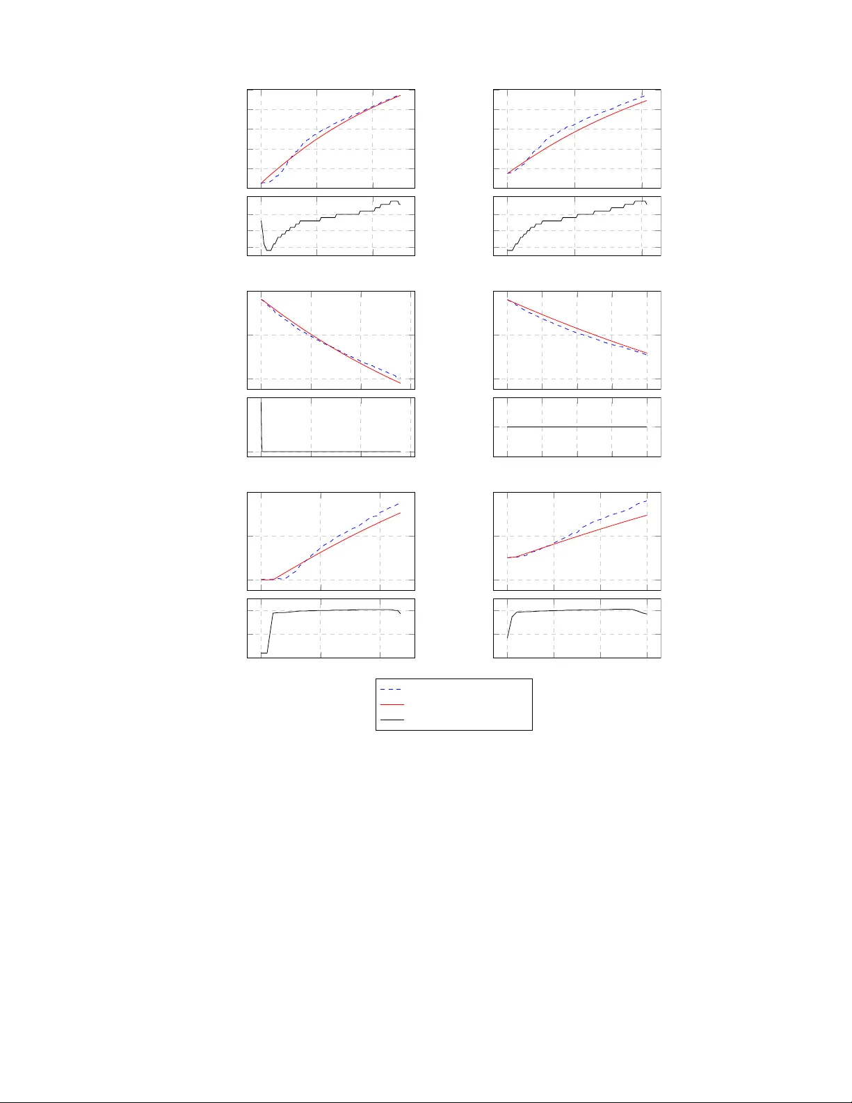
A p olynomial-time sc heduling approac h to minimise idle energy consumption: an application to an industrial furnace Ond ˇ rej Benedikt a,b , Baran Alik o¸ c a , P ˇ rem ysl ˇ S ˚ uc ha a , Sergej ˇ Celik ovsk´ y c and Zden ˇ ek Hanz´ alek a a Czec h Institute of Informatics, Robotics and Cyb ernetics, Czech T ec hnical Univ ersity in Prague, Czech Republic b F aculty of Electrical Engineering, Czec h T echnical Univ ersity in Prague, Czech Republic c Czec h Academy of Sciences, Institute of Information Theory and Automation, Czech Republic AR TICLE HISTOR Y Compiled Decem b er 17, 2020 ABSTRA CT This article presen ts a no ve l scheduling approac h to minimise the energy consump- tion of a machine during its idle p eriods. In the scheduling domain, it is common to mo del the b ehaviour of the machine by deﬁning a small set of machine mo des, e.g. “on”, “oﬀ ” and “stand-by”. Then the transitions b et ween the mo des are repre- sen ted by a static transition graph. In this pap er, we argue that this type of mo del migh t b e to o restrictiv e for some types of machines (e.g. the furnaces). F or such mac hines, w e prop ose to employ the complete time-domain dynamics and integrate it into an idle energy function. This wa y , the scheduling algorithm can exploit the full kno wledge about the mac hine dynamics with minimised energy consumption en- capsulated in this function. In this paper, we study a scheduling problem, where the tasks characterised by release times and deadlines are scheduled in the given order suc h that the idle energy consumption of the machine is minimised. W e show that this problem can b e solv ed in p olynomial time whenever the idle energy function is conca ve. T o highlight the practical applicability , we analyse a heat-intensiv e system emplo ying a steel-hardening furnace. W e derive an energy optimal control law, and the corresponding idle energy function, for the bilinear system model approximating the dynamics of the furnace (and p ossibly other heat-intensiv e systems). F urther, w e prov e that the idle energy function is, indeed, concav e in this case. Therefore, the prop osed scheduling algorithm can b e used. Numerical exp eriments show that b y using our approach, combining b oth the optimal control and optimal scheduling, higher energy savings can b e achiev ed, compared to the state-of-the-art scheduling approac hes. KEYW ORDS Sc heduling; energy optimisation; op erational research; optimal control; electric furnaces. 1. In tro duction The mac hines in heat-intensiv e pro cesses (such as f urnaces) are highly energy- demanding, and therefore their energy consumption optimisation usually pro vides a Corresponding author O. Benedikt. Email: benedond@fel.cvut.cz © 2020. This manuscript version is made av ailable under the CC-BY-NC-ND 4.0 license. signiﬁcan t reduction in pro duction costs. In this w ork, w e fo cus on the idle energy consumption optimisation, which has b een widely studied in recent years (see, e.g. Guto wski et al. 2005; Mouzon et al. 2007; Shrouf et al. 2014; Gahm et al. 2016; Che et al. 2017b; Abik arram et al. 2019). The research presented in this paper is inspired b y a heat-intensiv e pro duction pro cess from ˇ Sk o da Auto. There, steel hardening is p erformed in electric v acuum furnaces, whic h require high pow er input to reac h and main tain the sp eciﬁc op erating temp erature. In this pro duction line, all furnaces are heated to the op erating temp erature at the b eginning of the week and turned oﬀ at its end. Ho wev er, this strategy is very wasteful b ecause a considerable amount of energy is consumed for heating even during the p erio ds when no material is b eing pro cessed. The problem of energy-w asting during prolonged idle p erio ds is not speciﬁc only to this particular plant. Similar observ ations ha ve already b een made in other companies as w ell (Mouzon et al. 2007). A common approac h in the area of the idle energy consumption optimisation is to deﬁne a set of mac hine mo des, t ypically “oﬀ ”, “on”, and “stand-b y” (Mouzon et al. 2007; Shrouf et al. 2014; Che et al. 2017b; Abik arram et al. 2019). The feasible tran- sitions b et w een the mo des are then represen ted by a static tr ansition gr aph deﬁning the time and energy needed to switc h from one mode to another and thus describing the machine dynamics to some extent. In this pap er, w e argue that this type of mo del migh t be too restrictiv e for some t yp es of machines (e.g. the furnaces). F or such ma- c hines, we prop ose to employ the complete time-domain b ehaviour of the mac hine, when av ailable, in contrast to the use of the ﬁnite n umber of stand-b y mo des as in the existing literature. The relation b etw een the length of the idle p erio d and the p ossible minimal energy consumption is then represented by the id le ener gy function , whic h is used by the prop osed scheduling algorithm. This wa y , the whole energy minimisation problem is decomposed in to t wo independent optimisation problems: (i) determination of the idle energy function and (ii) optimal sc heduling of the tasks. F or the scheduling part, w e examine a single machine problem where tasks are c har- acterised b y release times, pro cessing times, and deadlines while the ob jectiv e is to minimise the idle energy consumption. Besides, we assume a ﬁxed order of tasks. The reason for this assumption is that the single machine problem with release times and deadlines is already N P -hard (Garey and Johnson 1977). Therefore, it is reasonable to solv e the entire pro duction problem by a heuristic. In this case, a decision con- cerning the order of tasks and their assignment to mac hines is often determined by a lo cal-searc h or meta-heuristic. These tec hniques can emplo y the sc heduling approach prop osed in this pap er for ﬁnding the optimal start times of the tasks given their order. W e prov e that whenev er the idle energy function is concav e, the scheduling problem can b e solv ed in p olynomial time by reduction to the shortest path problem. The main adv an tage of this transformation is that the size of the reduced problem is indep enden t of the length of the sc heduling horizon. The determination of the idle energy function is sp eciﬁc to the considered machine. In this paper, we tak e as an example electric furnaces widely used in industrial pro- duction lines such as steel hardening and glass temp ering, op erating at a sp eciﬁed temp erature. Using the Pon tryagin’s minimum principle (PMP) to analyse a realistic bilinear mo del of the contin uous-time furnace dynamics, we prov e that the energy- optimal con trol la w during an y idle p erio d is to switch from zero input p ow er (co ol- ing) to the maximum applicable input p o wer (maximal heating) at some conv enient switc hing time. This optimal con trol law is then shown to result in the concavit y of the idle energy function, which enables to employ the prop osed optimal sc heduling algorithm. The theoretical approac h and ﬁndings are v alidated through a case study 2 in vestigating an industrial furnace in a real pro duction line. 1.1. R elate d work Concerning the researc h of energy-eﬃcient manufacturing systems, one of the ﬁrst analyses in this area was p erformed by Mouzon et al. (2007), who observed that a sig- niﬁcan t amount of energy could b e sav ed by managing the state of the machine. They prop osed several dispatching rules for online pro duction, considering op er ating and id le states of the machine. Sp eciﬁcally , rules were devised to turn the non-b ottleneck mac hines oﬀ when they w ere idle for a certain amount of time. Exp erimen tal results sho wed that, compared to the worst-case p olicy (no switc hing), substantial energy sa vings could b e ac hieved. This research laid the foundations for further works inv es- tigating the minimisation of (idle) energy in pro duction. Often, following the example of Mouzon et al., authors consider only a simple case with t w o states, the pr o c ess- ing (op erational) state and oﬀ state. That is also the case in the work of Che et al. (2017a), who prop osed a mixed-integer linear programming (ILP) model and heuristics for bi-ob jectiv e minimisation of the energy and maximum tardiness. Another example can b e found in the w ork of Zhou et al. (2018), who prop osed a mathematical mo del and a diﬀerential ev olution algorithm for a parallel batch pro cessing mac hine sc hedul- ing problem considering minimisation of the mak espan and total energy consumption. Tw o states of the batc h processing mac hine were assumed for the modelling, namely the pr o c essing and id le state. Angel et al. (2012) analysed a single mac hine problem with tasks characterised b y release times and agreeable deadlines and show ed that the problem of idle energy minimisation can be solv ed in polynomial time when only on-oﬀ switc hing is considered. Mac hines c haracterised b y three states ( pr o c essing , id le , and shutdown ) w ere studied by both Shrouf et al. (2014) and Aghelinejad et al. (2018), who addressed energy minimisation under v ariable energy prices. A common asp ect of all previously men tioned w orks is that the dynamics of the machine is simpliﬁed to several constants (represen ting the transition times/costs betw een pairs of modes) only . Contrary to that, we sho w that by using a more precise mo del of the machine dynamics, higher energy savings can b e ac hiev ed. Our claim is supp orted b y a case study examining a heat-in tensive system emplo ying a steel-hardening furnace. Regarding sc heduling for heat-in tensive production systems and industrial furnaces, the literature is still very sparse. Some authors ha ve studied re-heating furnaces (Zhang et al. 2002; T ang et al. 2014), whic h are used to heat steel slabs to a sp eciﬁed temp er- ature before they en ter the next pro duction stage. Typically , the duration whic h the slabs sp end inside the furnace (i.e. the pro cessing time), and the sequence of the slabs are optimised. Ha ¨ ıt and Artigues (2011) studied the problem where the metal is melted in several induction furnaces. The melting time can b e shortened b y increasing the in- put p ow er. In con trast, the processing time, as well as the temperature, are sp eciﬁed in our case to ensure the desired qualit y of the pro duct. Liu et al. (2018) addressed a glass production ﬂow-shop problem, modelling mu ltiple stages, and optimising the mak espan and total energy consumption. Ho wev er, only the pr o c essing and id le states w ere considered to approximate the furnace dynamics in the scheduling mo del. In addition to the manufacturing processes men tioned previously , the research on p o w er-saving states has a broad base in the domain of em b edded systems, where energy sa vings are crucial to prolonging the battery life (Irani et al. 2003; Baptiste et al. 2012; Gerards and Kuper 2013). The considered devices typically hav e only a small num b er of p o w er-saving states (Gerards and Kup er 2013), whic h are sp eciﬁed 3 b y the manufacturer. Sometimes authors assume only the pr o c essing state and the oﬀ- state (Irani et al. 2003; Baptiste et al. 2012). The studied problems commonly lead to online sc heduling algorithms because of their real-time c haracter or uncertain ties in the arriv al times of the tasks. In contrast to embedded systems, the dynamics of machines in pro duction lines, e.g. for the heat-intensiv e systems inv estigated in our case study , is typically muc h slow er. Th us, by assuming only on and oﬀ states for such machines, the idle p erio ds b etw een t w o consecutiv e tasks w ould need to b e very long to make the transitions p ossible. Another diﬀerence is the p ossibilit y of solving the pro duction problems oﬄine with resp ect to known, or a priori appro ximated, parameters of the tasks and the identiﬁable dynamic behaviours. How ever, despite all diﬀerences, some concepts originating from the domain of em b edded systems are general and can still b e used ev en for pro duction scheduling. F requently , the idle energy consumption is captured b y an id le ener gy function , E : R ≥ 0 → R ≥ 0 , mapping the length of the idle p erio d to energy consumption (Gerards and Kup er 2013). Suc h a function E is t ypically assumed to be non-decreasing piecewise-linear concav e where each linear segmen t corresp onds to a single p ow er-saving state. Adopting this concept, we mainly prop ose a new p olynomial-time scheduling algorithm, also suitable for pro duction line mac hines whose dynamics can b e captured b y a concav e idle energy function. 1.2. Contributions and outline The main contribution of this pap er is t wofold. First, w e prop ose a new p olynomial sc heduling algorithm using the concept of the idle energy function. Second, w e sho w that the idle energy function can b e used to b etter represent the dynamics of the mac hine compared to the approaches that are just approximating it with few states only . As the exp erimen tal results show, w e can achiev e m uc h better energy sa vings. F urther, we list the particular con tributions of our article in the context of the present related w orks: (1) W e deﬁne the problem of idle energy consumption minimisation for a single mac hine scheduling with release times, deadlines, and the ﬁxed order of tasks where the consumption of the machine is deﬁned by the idle energy function (Section 2). (2) W e suggest decomp osing the studied problem to (i) the determination of the idle energy function with resp ect to the machine dynamics, and (ii) the optimal sc heduling of tasks. (3) W e show that the scheduling problem can b e solved in O ( n 3 ), where n is the n umber of tasks, assuming that the idle energy function is concav e (Section 3). T o the b est of our knowledge, the closest work that can b e adapted to our problem is the algorithm prop osed for a ﬁxed sequence of tasks in (Aghelinejad et al. 2019). The complexity of their algorithm is O ( | H | 2 n ), where | H | is the length of the sc heduling horizon. Since for practical applications | H |  n , our approach exhibits a b etter complexity (Section 6.3). (4) Utilising a bilinear system appro ximation of furnace dynamics, we prop ose an energy-optimal con trol la w for ﬁxed idle perio d lengths and sho w that the idle energy function under this con trol law is concav e (Section 4). (5) Com bining the sc heduling approac h and the idle energy function deriv ed for a real industrial furnace at ˇ Sk o da Auto (in Section 5), we verify the proposed approac h on a set of instances and sho w (in Section 6.2) that the prop osed solution provides signiﬁcantly less energy consumption as compared with the 4 existing modelling approach based on explicit mo delling of the machine mo des (Mouzon et al. 2007; Shrouf et al. 2014; Che et al. 2017b; Abik arram et al. 2019). The rest of the article is organised as follows. Section 2 pro vides the problem de- scription and assumptions. In Section 3, the dominant structures in schedules are iden tiﬁed, and it is shown that the sc heduling problem can be solv ed in p olynomial time b y ﬁnding the shortest path in a directed acyclic energy graph. Section 4 addresses the mo delling of the furnace; a bilinear mo del is describ ed, and the energy-optimal con trol law is derived. The case study in Section 5 describ es a real furnace used in the pro duction; bilinear mo del parameters are iden tiﬁed, and the idle energy func- tion is deriv ed. The case study is follow ed by Section 6, whic h shows the results of the n umerical sc heduling exp erimen ts using the iden tiﬁed model of the real furnace in contrast to the state-of-the-art mo delling techniques assuming a ﬁnite num b er of mac hine mo des. Finally , Section 7 concludes the article. 2. Problem statemen t W e study a sc heduling problem denoted 1 | r j , ˜ d j , ﬁxed order | Σ E , i.e. the minimisation of the idle energy consumption on a single machine where the order of the tasks is ﬁxed. F ormally , let T = { 1 , 2 , . . . , n } denote the set of tasks sorted according to the giv en order. Each task i ∈ T is characterised by three integers: release time r i ∈ Z ≥ 0 , deadline ˜ d i ∈ Z > 0 , and pro cessing time p i ∈ Z > 0 , suc h that r i + p i ≤ ˜ d i ∀ i ∈ T . A schedule is deﬁned by vector of start times s = ( s 1 , s 2 , . . . , s n ) ∈ R n ≥ 0 . A fe asible sche dule is such a schedule that satisﬁes the follo wing constraints. (C1) Eac h task i is pro cessed within its execution time windo w [ r i , ˜ d i ]. (C2) The pro cessing order of the tasks is given and ﬁxed. (C3) A t most, a single task is pro cessed at one time. (C4) The pro cessing is done without preemption. F or the rest of this work, when we talk ab out a sc hedule, we alwa ys mean a feasible sc hedule. W e assume that the mac hine is turned on (e.g. heated to the op erating temperature from oﬀ state in case of a furnace) just b efore the ﬁrst task is pro cessed, and it is turned oﬀ immediately after the last task is pro cessed. When the machine is oﬀ , the p o w er consumption is zero. Costs for turning the mac hine on and sh utting it oﬀ are constan t and cannot b e optimised. When a task is pro cessed, the machine operates in the pro cessing state given by the respective technological pro cess (e.g. the furnace is heated to the op erating tem- p erature, whic h is the same for all tasks). Therefore, energy consumption cannot b e optimised in this case, as w ell. How ever, during the idle p erio ds, the machine can c hange its state to lo wer the energy consumption (i.e. the temp erature of the furnace can b e low ered to sav e energy). At the end of the idle p erio d, the machine needs to b e switched back to the pro cessing state b efore the next task is pro cessed. The ob jectiv e is to ﬁnd start times s , such that the idle energy consumption E total ( s ), i.e. the total energy consumption during idle p erio ds, is minimised. An id le p erio d is deﬁned as the duration b et w een the completion time of a task and start time of the follo wing one. Since the execution order of the tasks is ﬁxed, w e can assume that the tasks are sorted in the giv en order, i.e. s i + p i ≤ s i +1 ∀ i ∈ { 1 , 2 , . . . , n − 1 } . 5 Then, the ob jective can b e written as min s E total ( s ) = min s n − 1 X i =1 E ( s i +1 − ( s i + p i )) , (1) where E : R ≥ 0 → R ≥ 0 represen ts the id le ener gy function , whic h enco des the rela- tionship b et ween the idle p erio d length and the consumed energy (taking into accoun t v arious p o w er-savings). The idle energy function is further discussed in Section 4.3, and a real example for an industrial furnace is sho wn in Figure 7 in Section 5. Note that because of the ﬁxed order, release times and deadlines can b e propagated. Sp eciﬁcally , taking tasks from left to right, release times can b e shifted suc h that r i := max { r i − 1 + p i − 1 , r i } , ∀ i ∈ { 2 , 3 , . . . , n } , (2) and taking the tasks from righ t to left, deadlines can b e adjusted suc h that ˜ d i := min { ˜ d i +1 − p i +1 , ˜ d i } , ∀ i ∈ { n − 1 , n − 2 , . . . , 1 } . (3) If there exists a task such that its propagated execution window is shorter than its pro cessing time, then the instance does not ha v e a feasible solution for the giv en order. F or the rest of this article, we assume that release times and deadlines are propagated and a feasible solution exists. 3. Sc heduling algorithm and complexit y analysis In this section, we show that 1 | r j , ˜ d j , ﬁxed order | Σ E can b e solved in p olynomial time under the assumption that the energy function E is concav e. Note that if the order w as not ﬁxed, the problem would b e N P -hard b ecause its underlying problem 1 | r j , ˜ d j |− is N P -complete in a strong sense (Garey and Johnson 1977). A sp ecial version of the problem studied here was addressed by Gerards and Kup er (2013), who assumed a so-called fr ame-b ase d system , i.e. a system where r i = ( i − 1) · T and ˜ d i = i · T for some constan t n umber T . In frame-based systems, execution windo ws of the tasks do not ov erlap. Gerards and Kup er show ed that idle energy minimisation in frame-based systems can b e done in p olynomial time, assuming that the idle energy function is conca ve. W e extend their result to 1 | r j , ˜ d j , ﬁxed order | Σ E , i.e. to systems with arbitrary release times and deadlines, assuming that the execution order of the tasks is ﬁxed. F urther, w e describe the structure of the ener gy gr aph , and sho w that 1 | r j , ˜ d j , ﬁxed order | Σ E can b e solved by ﬁnding the shortest path in that graph. But ﬁrst, w e provide necessary deﬁnitions and show that only sc hedules in a sp ecial form (so-called blo ck-form sche dules ) can b e assumed for the optimisation. 3.1. Deﬁnitions A basic structure that appears in the feasible schedules is called a blo ck of tasks or simply blo ck , and is widely used; see, e.g. Baker and T rietsch (2009) or Baptiste et al. (2012). 6 Deﬁnition 3.1 (Blo ck of tasks) . A sequence of tasks B = ( b 1 , . . . , b m ), which are sc heduled on the same mac hine, is called a blo c k of tasks if the follo wing prop erties hold: s b i + p b i = s b i +1 , ∀ i ∈ { 1 , 2 , . . . , m − 1 } , (4) ∀ i ∈ T \ B : ( s i + p i < s b 1 ) ∨ ( s i > s b m + p b m ) . (5) Prop ert y (5) states that blo ck B is maximal, i.e. it cannot be extended to the left or righ t. Ev ery feasible sc hedule is comp osed of blocks of tasks, whic h are separated b y idle interv als. Blocks are, therefore, fundamen tal building elements out of whic h the resulting sc hedule is created. Ev en though all schedules are comp osed of blo c ks of tasks, some sc hedules are sp ecial in a certain sense. W e call them blo ck-form sche dules . Deﬁnition 3.2 (Block-form schedule) . A schedule consisting of k blo cks B 1 , B 2 , . . . , B k is in the blo ck form if each block of tasks B j con tains at least one task, which starts at its (propagated) release time or ends at its (propagated) deadline; such a task is called the supp ort of blo c k B j . Thanks to the prop erties of the block-form schedules, the idle energy optimisation can b e made simple, as shown in Section 3.2 and Section 3.3. 3.2. Dominanc e of blo ck-form sche dules In this section, we show that blo c k-form schedules w eakly dominate all other sc hedules. T o prov e this, we utilise the following lemma. Lemma 3.3. Given a c onc ave id le ener gy function E : R ≥ 0 → R ≥ 0 , for 0 ≤  ≤ x ≤ y it holds that E ( x −  ) + E ( y +  ) ≤ E ( x ) + E ( y ) . (6) Pr o of. Prop ert y (6) is directly implied by the concavit y of E , see Gerards and Kup er (2013). Lemma 3.3 implies that, in the case of having tw o idle p erio ds x and y , energy E ( x ) + E ( y ) decreases or remains the same ev en if the shorter idle p erio d of length x is reduced on b ehalf of the longer idle p erio d of length y . Then, w e hav e the follo wing theorem. Theorem 3.4. Given a c onc ave id le ener gy function E , for every fe asible sche dule S 1 deﬁne d by start times s 1 , ther e exists a fe asible sche dule S 2 deﬁne d by start times s 2 , such that S 2 is in a blo ck form and E total ( s 1 ) ≥ E total ( s 2 ) . Pr o of. If S 1 is already in a blo c k form, nothing has to be done. Otherwise, S 1 consists of k blocks { B 1 , B 2 , . . . , B k } = B ﬁxed ∪ B free , B ﬁxed ∩ B free = ∅ , where B ﬁxed is the set of blocks that contain at least one supp ort, and B free are the blo c ks without supp orts. The blocks in B ﬁxed will not b e mo v ed, while the blo c ks in 7 B free will b e shifted to gain a support. By shift , we mean adding a non-zero constan t to all start times of the tasks in the blo c k. Let us assume that there is an inﬁnitely long idle perio d before the ﬁrst blo c k in S 1 and after the last one. Now, ev ery blo ck is separated from the other blo cks by t wo idle p eriods (b efore and after the blo ck). Let us take an arbitrary blo c k B ∈ B free . Since it do es not con tain a supp ort, it can b e shifted. The direction of the shift can b e selected according to Lemma 3.3 such that the idle energy consumption does not increase (i.e. shift the blo c k suc h that the shorter neigh b ouring idle p erio d decreases its length). Note that the leftmost (righ tmost) block is alwa ys shifted righ t (left) to prolong the time when the machine is oﬀ (idle energy consumption do es not increase). After the blo c k is shifted as m uch as p ossible, there are t wo p ossible outcomes. (1) Some task i ∈ B reaches its release time or deadline. In this case, blo ck B gains a support and joins B ﬁxed ; the cardinalit y of B free decreases b y one. (2) Blo c k B reac hes its neigh b ouring blo c k B neigh . In this case, blo ck B joins its neigh b ouring blo c k. If B neigh ∈ B ﬁxed , then B gains a supp ort and joins B ﬁxed . Otherwise, B free := ( B free \ { B , B neigh } ) ∪ { B ⊕ B neigh } , i.e. B and B neigh are joined (op erator ⊕ ). Anyw ay , the cardinality of B free decreases b y one. If cases 1. and 2. happ en at the same time, b oth B and B neigh gain a supp ort, join B ﬁxed , and the cardinalit y of B free decreases b y at least one. It can be seen that after one shift, the cardinality of B free decreases, and the idle energy consumption do es not increase (by Lemma 3.3). By iteratively shifting the blo c ks without supp orts, ev ery blo ck will even tually join B ﬁxed . Since there are at most n blo c ks in B free at the b eginning, and the cardinality of B free decreases after eac h shift, B free will b e empty after at most n iterations. Also, there are at most n tasks in eac h blo c k. Therefore, each shift can b e done in O ( n ) steps (shifting one task after another). Hence, the transformation can b e done in O ( n 2 ) steps. Schedule S 2 is then giv en by the start times of the tasks in B ﬁxed . Theorem 3.4 shows that it is suﬃcien t to optimise only ov er schedules in the blo c k form. 3.3. Finding an ener gy-optimal blo ck-form sche dule Here w e sho w ho w the schedules can b e represented as paths in an orien ted directed acyclic ener gy gr aph . The graph-based approac h w as originally introduced for frame- based systems b y Gerards and Kup er (2013), but since the release times and deadlines in their frame-based systems do not ov erlap, the graph had a very simple structure. In our case, w e need to non-trivially extend the idea, relying on Theorem 3.4. By Deﬁnition 3.2, eac h blo c k of a block-form sc hedule contains at least one support. The main idea leading to a graph-based approach is to represen t the supp orts of the sc hedule by nodes of the energy graph. In the following, w e will show that paths in the energy graph can be associated with the blo c k-form schedules and that the shortest path corresp onds to the optimal blo ck-form schedule. Our extended v ersion of the energy graph can b e represented as a triplet G = ( V G , E G , c ), where V G is set of its vertices, E G is set of its oriented edges, and c : 8 E G → R ≥ 0 is the cost function. F or each task i ∈ T , w e deﬁne vertices v r i and v ˜ d i represen ting situations when task i starts at its release time and ends at its deadline, resp ectiv ely . Let start( v x i ) b e the actual start time of the task i represen ted by vertex v x i , i.e. start( v x i ) = ( r i , if x is r , ˜ d i − p i , if x is ˜ d. (7) F urthermore, let us deﬁne t wo additional dumm y v ertices, the starting v ertex v s and the ending v ertex v e . W e will deﬁne the edges in suc h a wa y that the paths b et ween v s and v e represen t blo ck-form schedules. The set of edges E G consists of three types of edges, E G = E (1) G ∪ E (2) G ∪ E (3) G , where E (1) G = n ( v s , v x i )   i ∈ T , x ∈ { r, ˜ d } suc h that the partial schedule giv en by s i := start( v x i ) , s i 0 := s i − i − 1 X k = i 0 p k ∀ i 0 ∈ { 1 , 2 , . . . , i − 1 } is feasible o , (8) E (2) G = n ( v x i , v e )   i ∈ T , x ∈ { r, ˜ d } suc h that the partial schedule giv en by s i := start( v x i ) , s i 0 := s i + i 0 − 1 X k = i p k ∀ i 0 ∈ { i + 1 , i + 2 , . . . , n } is feasible o , (9) E (3) G = n ( v x i , v y i 0 )   i ∈ T , i 0 ∈ T , i < i 0 , x, y ∈ { r , ˜ d } and ∃ k ∈ { i, i + 1 , . . . , i 0 − 1 } such that the partial schedule given b y s i := start( v x i ) , s i 0 := start( v y i 0 ) , s a := s i + a − 1 X l = i p l ∀ a ∈ { i + 1 , i + 2 , . . . , k } , s b := s i 0 − i 0 − 1 X l = b p l ∀ b ∈ { k + 1 , . . . , i 0 − 1 } is feasible o . (10) In E (1) G , edges connect the starting v ertex v s and v ertex v x i , x ∈ { r , ˜ d } , i ∈ T , asso ciated with task i . Each edge represents the situation when task i is the supp ort and tasks { 1 , 2 , . . . , i − 1 } are aligned to the righ t, joining the blo ck supp orted b y task i , see Figure 1(a). Similarly , edges in E (2) G link v x i , x ∈ { r , ˜ d } , i ∈ T , with the ending vertex v e . Each edge represents the situations when task i is the supp ort, and tasks { i + 1 , i + 2 , . . . , n } are aligned to the left, joining the blo c k supp orted by i , see Figure 1(b). Finally , set E (3) G represen ts situations when there are tw o blo cks of tasks supp orted by i and i 0 , resp ectively . All the tasks { i + 1 , i + 2 , . . . , k } are aligned to the left and join the blo c k supp orted b y i and tasks { k + 1 , k + 2 , . . . , i 0 − 1 } are aligned to the righ t and join the blo c k supp orted b y task i 0 , see Figure 1(c). No w, w e deﬁne the cost function c . W e set the costs of edges in E (1) G and E (2) G to zero b ecause the tasks represented by these edges are processed without any idle p erio ds. The costs of edges in E (3) G corresp ond to the idle energy consumption b etw een tw o blo c ks of tasks. Even though there migh t be multiple p ossible w a ys to schedule the 9 i − 1 . . . 1 i r i i + 1 . . . n i r i ˜ d i r i i + 1 . . . k k + 1 . . . i 0 − 1 t f  v ˜ d i , v r i 0  i i 0 (a) (b) (c) Figure 1. Examples of the partial schedules corresp onding to the edges b etw een (a)  v s , v r i  , (b)  v r i , v e  , and (c)  v ˜ d i , v r i 0  . tasks b etw een the tw o supp orts, the pro cessing time of eac h task is assumed to b e constan t and so the length of the idle p eriod is in v ariant for a ﬁxed pair of supp orts. Let us denote the length of the idle perio d b et ween blo cks supp orted b y v x i and v y i 0 , where i 0 > i , by t f ( v x i , v y i 0 ), deﬁned b y t f ( v x i , v y i 0 ) = start( v y i 0 ) − (start( v x i ) + p i ) − i 0 − 1 X k = i +1 p k . (11) No w, the cost function can b e deﬁned in the follo wing wa y: c ( e ) = ( 0 , if e ∈ E (1) G ∪ E (2) G , E ( t f ( v x i , v y i 0 )) , if e = ( v x i , v y i 0 ) ∈ E (3) G . (12) Explanatory example. T o illustrate the energy graph, let us consider an arbitrary conca ve idle energy function E and four tasks characterised by parameters giv en in T able 1. The corresp onding energy graph is shown in Figure 2. Each edge e is lab elled b y its cost c ( e ), deﬁned by (12). Note that there is no edge b et w een v s and v r 3 b ecause if task 3 started at its release time, it w ould not be p ossible to execute the previous tasks without introducing an idle p erio d ( ˜ d 2 = 40 < 45 = r 3 ). But in that case, the previous tasks w ould form a diﬀeren t block, having its own supp ort. Therefore, edge ( v s , v r 3 ) do es not bring an y additional useful information. The situation is similar for other ‘missing’ edges. T able 1. Example task parameters. i 1 2 3 4 r i 0 15 45 80 ˜ d i 20 40 70 100 p i 10 15 5 10 The connection b et ween the paths in the energy graph and blo c k-form schedules is explained b y the following t wo lemmas. Lemma 3.5. F or every blo ck-form sche dule S , ther e exists a p ath in the c orr esp ond- ing ener gy gr aph, such that length of the p ath e quals the id le ener gy c onsumption of sche dule S . Pr o of. This is assured b y the structure of the energy graph. Given a block-form sc hedule with blo ck s B 1 , B 2 , . . . , B k and their supp orts a 1 , a 2 , . . . , a k , the corresp ond- 10 v s v r 1 v r 2 v r 3 v r 4 v ˜ d 1 v ˜ d 2 v ˜ d 3 v ˜ d 4 v e 0 0 0 E (5) E (15) E (10) E (5) E (15) E (35) E (5) E (25) E (30) E (40) E (10) E (20) 0 0 E (30) Figure 2. Energy graph constructed for the tasks sp eciﬁed by T able 1. ing path in the energy graph is v s , v x ( a 1 ) a 1 , v x ( a 2 ) a 2 , . . . , v x ( a k ) a k , v e , where x ( a i ) := ( r if a i starts at its release time , ˜ d if a i ends at its deadline . (13) No des on the path corresp ond to the supp orts of the individual blo cks, and b ecause the cost of each edge directly corresp onds to the idle energy consumption, the length of the path is the same as the idle energy consumption of the sc hedule. Lemma 3.6. F or every p ath P b etwe en the start no de v s and end no de v e in the ener gy gr aph, ther e exists a fe asible blo ck-form sche dule S , such that the id le ener gy c onsumption c ost of S is the same as the length of p ath P . Pr o of. Again, this is trivially given by the structure of the energy graph, where no des represen t supp orts of the blo c ks. According to (8)–(10), an edge b et w een tw o no des represen ting the supp orts is added only if there exists a feasible sc hedule of the tasks b et w een them. Finally , b y Lemmas 3.5 and 3.6, we see that problem 1 | r j , ˜ d j , ﬁxed order | Σ E can b e solved by ﬁnding the shortest path in a directed acyclic graph. The graph contains O ( n ) vertices and at most O ( n 2 ) edges. Whether edge e b elongs to the graph or not can be veriﬁed according to (8)–(10) in linear time O ( n ). Therefore, the n um b er of steps needed to build the graph is upper bounded b y O ( n 3 ). The shortest path itself can b e found in linear time with resp ect to the size of the graph by the dynamic programming (Cormen et al. 2001, sec. 24.2). So the ov erall complexity is b ounded by O ( n 3 ). Explanatory example (con tin ued). The sc hedule corresp onding to path v s , v ˜ d 1 , v r 3 , v r 4 , v e is depicted in Figure 3. It consists of three blo c ks, B 1 = (1 , 2), B 2 = (3), and B 3 = (4). Supports of these blo c ks are tasks 1, 3 and 4, resp ectively . Idle energy consumption of the schedule equals the sum of energy consumed during the ﬁrst idle perio d (from time 35 to time 45), plus energy consumed during the second idle p eriod (from time 50 to time 80). Remark 1. Note that edges in E (3) G migh t not imply one particular sc hedule of the tasks b et ween the supp orts. Therefore, for a given path, there migh t exist multiple feasible schedules with the same idle energy consumption. Similarly , as each blo c k 11 0 10 20 30 40 50 60 70 80 90 1 2 3 4 E (10) E (30) ˜ d 1 r 3 r 4 B 1 B 2 B 3 Figure 3. F easible schedule corresp onding to path v s , v ˜ d 1 , v r 3 , v r 4 , v e . migh t contain multiple supp orts, there might b e m ultiple diﬀeren t paths corresp onding to one blo c k-form sc hedule. Remark 2. The graph-based approach describ ed ab o ve can handle arbitrary concav e idle energy function, whic h is a common shap e of the idle energy function used in the literature (Irani et al. 2003; Gerards and Kup er 2013). Ho wev er, it is still an op en question if the problem would b e p olynomial even if the idle energy function was not conca ve but arbitrary . Remark 3. The energy graph could also b e used to ﬁnd the schedules minimising the num b er of idle p erio ds longer than 0. Such an application is useful when the stress of the mac hine caused by excessive switching needs to b e minimised. The problem reduces again to the shortest path problem. The structure of the graph remains the same, but the edges in E (3) G should b e lab elled by some p ositiv e constant, e.g. 1. Note that it is again p ossible to optimise only o ver the blo c k-form sc hedules because the shifts described in the pro of of Theorem 3.4 might join some blo cks but nev er split them. 4. Electric furnaces: mo delling, optimal con trol and energy function Up till no w, we ha ve discussed ho w to solve sc heduling problem 1 | r j , ˜ d j , ﬁxed order | Σ E , assuming that the energy function is giv en and con- ca ve. The ma jority of the existing papers addressing the idle energy optimisation assume that the dynamics of the machine is describ ed b y a static transition graph, and its parameters are giv en. Obtaining those parameters or the idle energy function can b e simple in some cases (e.g. for some hardw are components in the embedded systems, the parameters or the idle energy function can be extracted from the data provided b y the man ufacturer), but b ecomes quite c hallenging in others. Since the idle energy optimisation aims at a large v ariet y of mac hines ranging from pro cessors to h uge furnaces, it is not p ossible to pro vide a single approach for obtaining the parameters of the transition graph or the idle energy function. Therefore, w e concentrate on heat-in tensive systems that are the most frequently addressed in connection with the idle energy optimisation in pro duction. In this section, w e discuss the electric furnace mo dels and present a bilinear mo d- elling approach, which is sho wn to provide a go o d approximation of industrial elec tric furnace dynamics. F urther, the op en-loop control for minimum energy consumption during idle p erio ds, concerning the studied sc heduling problem, is giv en based on the considered bilinear system appro ximation. Then, we show that the idle energy function as an input to the scheduling problem is conca v e under the proposed approximation and con trol, thus conﬁrming the use of the ab o ve-proposed algorithm is correct. 12 4.1. A biline ar mo del appr oximation of furnac es Obtaining and identifying a reasonable physical mo del of an industrial furnace is usu- ally v ery diﬃcult due to unsp eciﬁed characteristics, imp erfections or degradation of insulation materials, and time/temp erature dep endency of the ph ysical parameters. Th us, instead of prop osing a physical mo del and identifying its parameters, it is usual in practice to approximate the furnace dynamics with reasonable linear and nonlinear mathematical mo dels; see, e.g. W ang and Spanos (2002) for a linear mo del, Mo on and Lee (2003) for a fuzzy system appro ximation, W ang et al. (1998) for a direction- dep enden t mo del, and Y u (2000); Chee Cho ok and T an (2007) for bilinear system appro ximations. Our decision to use the bilinear approximation of the furnace dynamics is motiv ated b y the existing literature. F or example, Derese and No dulus (1980) hav e rep orted that the bilinear model for heat-transfer pro cesses is more suitable than the linear model. Chee Cho ok and T an (2007) considered the iden tiﬁcation of a ﬁrst-order bilinear mo del for an electric tub e furnace and sho wed exp erimen tally that the bilinear mo del provides the most accurate description as compared with the linear and direction-dep enden t mo dels. Another adv an tage of the bilinear mo del is its simplicit y and w ell-understo o d b eha viour in the class of nonlinear systems. Th us, we also consider the approximation of the furnace dynamics similarly as in Chee Cho ok and T an (2007) with the bilinear mo del ˙ x ( t ) = − αx ( t ) + β u ( t ) − ρx ( t ) u ( t ) , x ( t ) ∈ R , u ( t ) ∈ [0 , ¯ u ] , α, β , ρ ∈ R > 0 (14) where u is the applied electric p ow er (in kilow atts), i.e. the input to the system, and x is the deviation of the furnace temp erature T f (in kelvins) from the constant ambien t temp erature T e , x ( t ) := T f ( t ) − T e , i.e. the v ariable to be controlled. The mo del (14) sligh tly diﬀers from that in Chee Cho ok and T an (2007), because w e additionally accommo date constraints on control and system parameters regarding the reality for furnaces. First, w e do imp ose the upp er b ound ¯ u on the admissible control p ow er, whic h is imp ortan t in practice. Second, based on ph ysical mo delling considerations, it is assumed in (14) that the system parameters α , β , and ρ are positive constan ts. That is due to Chee Cho ok and T an (2007), where Section IV provides successful iden tiﬁcation of α, β , ρ , resulting as p ositiv e n umbers for their furnaces op erational data. Note, that physical-principle-based mo delling provided in Chee Cho ok and T an (2007) actually giv es the following mo del ˙ T f ( t ) = 1 C f  − T f ( t ) − T e R + u ( t ) − K ( T 4 f ( t ) − T 4 e )  , (15) where C f is the thermal capacitance, R is the thermal resistance, and K is a constan t regarding the emissivit y of the furnace. Ob viously , C f , R, K > 0; as already noted, T e stands for the ambien t temperature, which is assumed constant since its p ossible v ariations are negligible compared to extremely high furnace temp eratures. Due to its complexit y , instead of (15) Chee Cho ok and T an (2007) study simpler bilinear mo del (14) and pro vide some argumen ts for such a simpliﬁcation. Indeed, there is a kind of trade-oﬀ: higher-order nonlinearity of (15) is replaced b y bilinear dep endence in (14), so rigorously (14) is not a simpliﬁcation or appro ximation of (15). Y et, as sho wn in the sequel, (14) can b e handled in an easier wa y , and some rigorous mathematical statemen ts can b e pro ved for it. Besides easier theoretical analysis, another argument 13 justifying replacement of (15) b y (14) giv en in Chee Cho ok and T an (2007) is that the nonlinearities that arise in heat-transfer pro cesses ma y b e represen ted by c haracter- istics that are similar to those of a bilinear system. In suc h a wa y , the curren t paper joins the existing literature mainstream represented b y Chee Cho ok and T an (2007) and will concentrate on the mo del (14) only . Note, that the constraints on α, β , ρ will hold for the electrical v acuum furnace, which is studied in Section 5 as a case study . As sho wn in Section 5.1 later on, these parameters α, β , ρ can b e quite precisely iden tiﬁed based on the real data, and the resulting estimates comply with the ab o ve assumptions. 4.2. Solving the or dinary diﬀer ential e quation with a disc ontinuous right-hand side Before formulating the main theorem of this section analysing the optimal con trol of system (14), let us brieﬂy recall the deﬁnition of the solution of the ordinary diﬀerential equation (ODE) with the p ossibly discontin uous righ t-hand side. This o verview is presen ted in a rather casual wa y; rigorous and detailed theory can b e found, e.g. in (Filipp o v 1988, Chapter 1). Indeed, as it will be seen, the optimal con trol is a discon tinuous function in time and thereby after substituting it into (14) one gets ODE with discon tinuous (in time v ariable) right-hand side. Namely , consider ODE ˙ x ( t ) = f ( x ( t ) , t ) , x ∈ R n . (16) The usual deﬁnition of the solution of (16) for its c ontinuous right-hand side f ( x, t ) is that the s olution x ( t ) is a contin uously diﬀerenti able function of time conv erting the ab o v e ODE into equality v alid for all times. As there are inﬁnitely man y such solutions, the sp eciﬁc unique solution is determined by the so-called initial c ondition x ( t 0 ) = x 0 , x 0 ∈ R n , t 0 ∈ R , (17) where t 0 , x 0 are giv en initial time and initial condition, respectively . The relations (16) and (17) are usually referred to as the initial value pr oblem , or Cauchy pr oblem . When the right-hand side of (16) is discon tinuous, the solution of (16) cannot b e con tinuously diﬀeren tiable in time. When the discontin uity is with respect to time only , the usual w ay to handle this situation is to deﬁne the solution in Car athe o dory sense ; namely , the initial v alue problem (16) and (17) is replaced by the following in tegral equation x ( t ) = x ( t 0 ) + Z t t 0 f ( x ( τ ) , τ )d τ , (18) where the solution x ( t ) is required to b e con tinuous only . Note, that the solution of the in tegral equation (18) automatically satisﬁes the initial condition (17) and, moreo ver, where x ( t ) is in addition contin uously diﬀerentiable, it implies the v alidit y of (16). As already noted, Caratheo dory approach helps to handle the discon tinuit y with resp ect to the time v ariable only . The discon tinuit y with respect to state v ariable x presents ev en more tough c hallenge and even more abstract solution is required, namely the so-called solution in the Fillip o v’s sense. In the subsequent analysis, all the time discontin uities will b e of the simplest kind, i.e. they will b e piecewise contin uous. In this case, Caratheo dory solution can also b e 14 obtained in the follo wing in tuitively clear wa y . Namely , ODE is solv ed together with the initial condition on the largest time interv al where f ( x, t ) is contin uous. When reac hing discon tinuit y p oin t t dc ∈ R , the resulting solution v alue x ( t dc ) is taken as the initial condition for the next time in terv al where f ( x, t ) is contin uous; ODE is solved again and this pro cedure can b e rep eated. Note that suc h an approach correctly represents realit y . In the case of furnace heat- ing, it means that discontin uous jump change of heating inﬂuences further developmen t of the temp erature, but the temp erature has to stay con tinuous even at the p oin t where heating in tensity exp eriences jump, see Figure 6. Obviously , suc h an understanding of the solution of the ODE with time discon tinuit y at its righ t-hand side is the only acceptable one from the natural and practical p oint of view. Putting it in diﬀeren t w ords, under quite mild and reasonable mathematical technical assumptions imp osed on the right-hand side f ( x, t ), there is a unique solution that satisﬁes ODE in a clas- sical sense everywhere except some isolated time momen ts, where this unique solution is at least contin uous. In other words, man y solutions are p ossible, but only one of them is ev erywhere at least contin uous. In the sequel, w e will use exactly the latter approach to obtain the unique solution of the initial v alue problem when heating intensit y (the input) is piecewise constant. Namely , we compute the solution to the initial v alue problem on time subin terv al where heating intensit y is constant. Then, at the time where heating intensit y jumps to a diﬀerent constan t v alue, w e use the terminal v alue of temp erature on the ﬁrst time subin terv al as the initial condition for the ODE solution on the next time subinterv al. 4.3. Minimum-ener gy c ontr ol and the r elate d id le ener gy function This subsection aims to study the optimal control of furnaces during an idle p eriod, based on the appro ximate bilinear mo del (14). Recall that our aim is to ﬁnd an energy-eﬃcient b eha viour of the furnace in an idle p erio d. Thus, we lo ok for an optimal control law, which minimises the p o wer consumption for an y ﬁxed idle perio d length. Then, our problem for furnaces turns in to ﬁnding a control minimising the p erformance index J ( u ) = Z t f 0 | u ( t ) | dt (19) whic h is called as minim um-control-eﬀort problem (Kirk 2004). Obviously , t f can b e considered as the idle p erio d length, i.e. ( s i +1 − ( s i + p i )) in (1). Then J ( u ) is the energy (in kilow att-hours) consumed during the corresp onding idle perio d, i.e. E ( s i +1 − ( s i + p i )) in (1). Note, that it is suﬃcien t to consider an open-lo op control to heat the furnace to the (close neighbourho o d of ) op erating temp erature at the end of the idle p erio d (assuming constan t am bient temp erature), whereas a closed-lo op con trol is necessary to maintain the op erating temp erature. Suc h a control strategy is actually common in pro cess con trol applications, e.g. see Figure 4 with the tempera- ture data of the real industrial furnace controlled to op erate at diﬀerent temp eratures in our case study . As we seek a con trol minimising energy consumption during the idle p eriods, w e give the follo wing theorem for the op en-lo op optimal con trol problem for the industrial furnaces whic h can b e mo delled as the bilinear system in (14). Theorem 4.1. Consider the fol lowing optimal c ontr ol pr oblem: minimise the p erfor- 15 manc e index (19) subje ct to c onstr aints x (0) = x ( t f ) = x 0 ∈ R , x 0 > 0 , (20) wher e x ( t ) is the solution of the system (14) and t f > 0 is a given ﬁxe d terminal time. F urther, assume that ( β − ρx 0 ) ¯ u − αx 0 > 0 , (21) wher e ¯ u is the upp er b ound on u ( t ) . Then ther e exists the unique optimal c ontr ol u ∗ ( t ) solving the ab ove-deﬁne d optimal c ontr ol pr oblem and this optimal c ontr ol takes the fol lowing form u ∗ ( t ) = ( 0 , ∀ t ∈ [0 , t sw ) ¯ u, ∀ t ∈ [ t sw , t f ] , (22) wher e t sw ∈ (0 , t f ) is the switching time. Final ly, t sw is the solution of the fol lowing e quation x 0 = exp (( − α − ρ ¯ u )( t f − t sw ))  x 0 exp( − αt sw ) − β ¯ u α + ρ ¯ u  + β ¯ u α + ρ ¯ u , (23) this solution exists and is unique for any given t f > 0 . F urthermor e, deﬁne d in such a way function t sw ( t f ) satisﬁes d t sw d t f = 1 − αx 0 ( β exp( αt sw ) − ρx 0 ) ¯ u . (24) Pr o of. P ontry agin’s minimum principle (PMP) is used (Kirk 2004). T o do so, realise that | u ( t ) | in (19) can b e replaced simply by u ( t ) b ecause u ( t ) > 0 ∀ t in (14). F urther, the appropriate Hamiltonian function for the performance index (19) and the system (14) is giv en by H ( x ( t ) , u ( t ) , ψ ( t )) = u ( t ) − αψ ( t ) x ( t ) + ψ ( t )[ β − ρx ( t )] u ( t ) (25) where ψ ( t ) represents the usual adjoin t v ariable. By PMP , the necessary conditions for u ∗ ( t ) to b e an optimal control are ˙ x ∗ ( t ) = ∂ H ( x ∗ , u ∗ , ψ ∗ ) ∂ ψ = − αx ∗ ( t ) + β u ∗ ( t ) − ρx ∗ ( t ) u ∗ ( t ) , (26a) ˙ ψ ∗ ( t ) = − ∂ H ( x ∗ , u ∗ , ψ ∗ ) ∂ x = ψ ∗ ( t )( ρu ∗ ( t ) + α ) , ψ (0) = ψ 0 ∈ R \ { 0 } , (26b) H ( x ∗ ( t ) , u ∗ ( t ) , ψ ∗ ( t )) = min u ∈ [0 , ¯ u ] H ( x ∗ ( t ) , u ( t ) , ψ ∗ ( t )) ∀ t ∈ [0 , t f ] ⇒ (26c) 16 u ∗ ( t ) + ψ ∗ ( t )[ β − ρx ∗ ( t )] u ∗ ( t ) = min u ∈ [0 , ¯ u ] ( u ( t ) + ψ ∗ ( t )[ β − ρx ∗ ( t )] u ( t )) ∀ t ∈ [0 , t f ] . (26d) Indeed, the b oundary conditions (20) of the inv estigated control problem are ﬁxed, so that ψ ( t ) can b e any nontrivial solution of the adjoint equation (26b). Before analysing the ab o v e necessary condition for the optimality , let us giv e the follo wing prop ert y useful later on. Namely , (26a) and (26b) can b e solved analytically giving that x ∗ ( t ) = exp  − αt − ρ Z t 0 u ∗ ( η ) dη   x 0 + β Z t 0 exp  αη + ρ Z η 0 u ∗ ( s ) ds  u ∗ ( η ) dη  , (27) ψ ∗ ( t ) = ψ 0 exp  αt + ρ Z t 0 u ∗ ( η ) dη  . (28) T o analyse (26a)–(26d) sub ject to the control constraint u ( t ) ∈ [0 , ¯ u ], consider the function φ ( ψ ∗ ( t ) , x ∗ ( t )) = ψ ∗ ( t )( β − ρx ∗ ( t )) + 1 (29) to in vestigate the minim um of the Hamiltonian with resp ect to u . F urther, realise that the necessary condition (26c)–(26d) implies that u ( t ) = ¯ u if φ ( ψ ∗ ( t ) , x ∗ ( t )) < 0; u ( t ) = 0 if φ ( ψ ∗ ( t ) , x ∗ ( t )) > 0; whereas for φ ( ψ ∗ ( t ) , x ∗ ( t )) = 0 it is alwa ys satisﬁed. As a consequence, the optimal con trol, if it exists, satisﬁes u ∗ ( t )      = ¯ u, for φ ( ψ ∗ ( t ) , x ∗ ( t )) < 0 = 0 , for φ ( ψ ∗ ( t ) , x ∗ ( t )) > 0 ∈ [0 , ¯ u ] , for φ ( ψ ∗ ( t ) , x ∗ ( t )) = 0 . (30) F urthermore, by (27) and (28) it holds that φ ( t ) = 1 − ψ 0 x 0 ρ + ψ 0 β exp  αt + ρ Z t 0 u ( η ) dη  − ψ 0 β ρ Z t 0 exp  αt + ρ Z η 0 u ( s ) ds  u ( η ) dη , dφ ( t ) dt = ψ 0 β ( α + ρu ( t )) exp  αt + ρ Z t 0 u ( η ) dη  − ψ 0 β ρ u ( t ) exp  αt + ρ Z t 0 u ( η ) dη  , (31) whic h implies dφ ( t ) dt = ψ 0 αβ exp  αt + ρ Z t 0 u ( η ) dη  . (32) No w, using (31) and (32) one concludes that φ (0) = ψ 0 ( β − ρx 0 ) + 1 , (33) 17 sign  dφ dt  = sign( ψ 0 ) , ψ 0 6 = 0 . (34) Note that by (34) φ ( t ) is obviously a strictly monotonous function. In such a wa y , φ ( t ) either v anishes at a single isolated p oin t only , or it never v anishes. As ψ 0 6 = 0, only the follo wing four options are p ossible for u ∗ ( t ) to b e optimal. (1) If ψ 0 > ( ρx 0 − β ) − 1 > 0, then φ (0) > 0 and dφ ( t ) dt > 0, ∀ t ≥ 0, which means φ ( t ) > 0, ∀ t ≥ 0. By (30), then u ∗ ( t ) ≡ 0. Ho w ever, it is clear from (27) that (14) with u ( t ) ≡ u ∗ ( t ) ≡ 0 do es not satisfy (20). (2) If ( ρx 0 − β ) − 1 > ψ 0 > 0, then φ (0) < 0 and dφ ( t ) dt > 0, ∀ t ≥ 0. By (30), then u ∗ ( t ) = ¯ u, t < t sw and u ∗ ( t ) = 0 , t > t sw . Ho wev er, this option is not possible b ecause ( ρx 0 − β ) > 0 contradicts the assumption (21) as α , ¯ u and x 0 are p ositiv e. (3) If ψ 0 < ( ρx 0 − β ) − 1 < 0, then φ (0) < 0 and dφ ( t ) dt < 0, ∀ t ≥ 0, which means φ ( t ) < 0, ∀ t ≥ 0. By (30), then u ∗ ( t ) ≡ ¯ u . How ever, by assumption (21) and by (27) it holds that x ( t f ) > x 0 . Th us, (20) is violated. (4) If ( ρx 0 − β ) − 1 < ψ 0 < 0, then φ (0) > 0 and dφ ( t ) dt < 0, ∀ t ≥ 0. By (30), then u ∗ ( t ) = 0 , t < t sw , u ∗ ( t ) = ¯ u, t > t sw ; t sw = α − 1 log (( ρx 0 ψ 0 − 1) / ( β ψ 0 )) . (35) Moreo ver, it can b e seen through some straigh tforward analysis that when ψ 0 ranges through (( ρx 0 − β ) − 1 , 0), the expression (( ρx 0 ψ 0 − 1) / ( β ψ 0 )) ranges through (1 , ∞ ), i.e. ψ 0 can alwa ys b e chosen in suc h a w ay that any t sw ∈ (0 , ∞ ) is p ossible. Summarising, the con trol satisfying PMP and (20) under assumption (21) should ha ve the form (35) for some suitable switc hing time t sw . T o conclude the pro of, it remains to show that there is a unique t sw ∈ [0 , t f ) such that (14) with u ( t ) ≡ u ∗ ( t ) given by (35) satisﬁes the b oundary conditions (20). Suc h a prop erty follo ws straigh tforwardly b y (27) and (21), moreov er, also by (27), the switching time t sw is the solution of x 0 = exp (( − α − ρ ¯ u )( t f − t sw ))  exp( − αt sw ) x 0 − β ¯ u α + ρ ¯ u  + β ¯ u α + ρ ¯ u . (36) Indeed, on the righ t-hand side of (36) there is a v alue of temp erature tra jectory x ( t ) at time t f obtained b y solving (14) on subin terv al [0 , t sw ) with initial condition x (0) = x 0 applying the input (applied p o w er) u ≡ 0 and then solving (14) with initial condition x ( t sw ) = exp( − αt sw ) x 0 and the input u ≡ ¯ u on subinterv al [ t sw , t f ]. Note, that t sw solving (36) exists and is unique for any giv en t f > 0. Indeed, the righ t-hand side of (36) is a smooth function of t sw and it is equal to exp ( − αt f ) x 0 < x 0 if t sw = t f and to exp (( − α − ρ ¯ u ) t f )  x 0 − β ¯ u α + ρ ¯ u  + β ¯ u α + ρ ¯ u > x 0 , if t sw = 0. The last inequalit y straigh tforw ardly holds thanks to the assumption (21) and exp (( − α − ρ ¯ u ) t f ) ∈ (0 , 1). As a consequence, there exists at least one t sw solving (36) thanks to the well-kno wn basic prop ert y of con tin uous functions. T o show that suc h t sw is unique, note that the right-hand side of (36) is strictly decreasing function 18 of t sw since its deriv ative with resp ect to t sw is ¯ u · exp(( − α − ρ ¯ u )( t f − t sw )) · ( ρx 0 exp( − αt sw ) − β ) , whic h is negative since b y the assumption (21) β > ρx 0 and ob viously ρx 0 > ρx 0 exp( − αt sw ) as α > 0 , t sw ≥ 0. In such a wa y , the v alue t sw solving (36) exists and is unique. Finally , to prov e (24) apply the well-kno wn formula to compute the deriv ative of the implicitly deﬁned function and p erform some straightforw ard, though lab orious computations. The pro of is complete. Remark 4. The assumption (21) is equiv alent to αx 0 / ( β − ρx 0 ) ∈ (0 , ¯ u ). The v alue αx 0 / ( β − ρx 0 ) is the constant trim control keeping the state x 0 as the equilibrium, i.e. x ( t ) ≡ x 0 and therefore the assumption (21) should b e v alid in any reasonable practical setting. Indeed, if the assumption (21) is to b e replaced b y ( β − ρx 0 ) ¯ u − α x 0 = 0, then the optimal control is u ∗ ( t ) = ¯ u, ∀ t ∈ [0 , t f ], i.e. as if t sw = 0 in (35). As such, ¯ u = αx 0 / ( β − ρx 0 ) is the trim control v alue that ensures x ( t ) ≡ x 0 ; practically , suc h a situation is not acceptable because any small p erturbation pushing the state to a v alue slightly lo wer than x 0 cannot b e comp ensated for. Remark 5. W e consider the optimal control law with the state constraint (20) b ecause a single op erating temp erature x 0 for the scheduling problem is considered. Deﬁnitely , the furnace temp erature is x 0 at the b eginning of each idle p erio d and should also b e x 0 at the end of the idle p erio d to execute the consecutive task. In fact, Theorem 4.1 can be easily extended to a more general case with boundary conditions of the form x (0) = x 0 , x ( t f ) = x f , x 0 > 0 , x f > 0 and, p ossibly , x 0 6 = x f . Let us ﬁnally sho w that the energy function of the idle p erio d length, for a fur- nace describ ed by the bilinear mo del (14) and optimally controlled as prop osed in Theorem 4.1, is conca ve. Theorem 4.2. The id le ener gy function E : R ≥ 0 → R ≥ 0 of system (14) under c ontr ol (22) assuming (21) is describ e d by e quation E ( t f ) = ¯ u · ( t f − t sw ( t f )) for any t f ∈ R ≥ 0 , wher e t sw ( t f ) is the function existing by (23) . Mor e over, E ( t f ) is c onc ave. Pr o of. Recall that ¯ u is constant maximal v alue of the applied electric p o wer in (14). Also recall from the pro of of Theorem 4.1 that t sw in con trol (22) applied to system (14) is uniquely determined with the implicit solution of (23) for given t f and ﬁxed parameters α , β , ρ , x 0 , and ¯ u . Th us, the energy consumption during an idle p erio d, i.e. idle energy function, can b e describ ed as E ( t f ) = ¯ u · ( t f − t sw ( t f )) . (37) Then, for conca vity of E ( t f ), it remains to sho w that ∂ 2 E ( t f ) ∂ t 2 f = − ¯ u d 2 t sw d t 2 f (38) is negativ e ∀ t sw . Substituting further diﬀeren tiation of (24) to (38) gives ∂ 2 E ( t f ) ∂ t 2 f = − α 2 β x 0 exp( αt sw ) ( ρx 0 − β exp( α t sw )) 2 d t sw d t f . (39) 19 T o prov e (39), ﬁrst note that by assumption (21), it holds β > ρx 0 and therefore, the denominator of the fraction in (39) is p ositiv e. The numerator α 2 β x 0 exp( αt sw ) is p ositive as well, since β > 0 b y deﬁnition (14) and x 0 > 0 by (20). Therefore, to pro ve that (39) is negative, it remains to show that (d t sw ) / (d t f ) > 0 ∀ t sw . By (21) we ha ve αx 0 < ( β − ρx 0 ) ¯ u , whic h also implies αx 0 < ( β exp( αt sw ) − ρx 0 ) ¯ u since α > 0 b y deﬁnition (14) and t sw ≥ 0. It follo ws that αx 0 ( β exp( αt sw ) − ρx 0 ) ¯ u < 1, which in turn pro ves that (d t sw ) / (d t f ) > 0. As a consequence, E ( t f ) is concav e, and the pro of is complete. By Theorem 4.2, we conclude that problem 1 | r j , ˜ d j , ﬁxed order | Σ E can b e solv ed in p olynomial time for furnaces that can b e mo delled as (14), and con trolled b y (22). In the following section, the prop osed approac h is shown on a real industrial electric furnace from ˇ Sk o da Auto. 5. Case Study: An industrial electric furnace ˇ Sk o da Auto has a pro duction line emplo ying a ModulTherm ® system by ALD, con- taining electric v acuum furnaces used for the steel hardening. The outer steel shells of the furnaces are cooled b y a cen tral cooling system of circulating water at ∼ 35 ° C to a void ov erheating of the system. Th us, w e can assume that the ambien t temp erature ( T e ) is constan t. The op erating temperature of the furnaces is set to 960 ° C for the hardening pro cess, which takes ab out 2 . 5 hours on av erage. The heating of the furnaces has a substantial energy demand across the whole pro duction line. In a normal regime, all furnaces are turned on and heated to the op erating temperature. The operating temp erature is preserved ev en if nothing is b eing pro cessed. T o inv estigate the p oten tial for energy savings, an exp erimen t has b een performed, during whic h the furnace was co oled to 600 ° C, and its steady-state p o w er consumption was measured. Afterwards, the furnace was heated back to the op erating temp erature again. Measured data are shown in Figure 4 (Du ˇ sek 2016). It can be seen that the steady-state pow er consumption for 600 ° C and 960 ° C is about 18 kW and 40 kW, resp ectively . Clearly , if the idle p erio d is long enough, signiﬁcant energy savings can b e achiev ed b y lo w ering the temperature of the furnace, i.e. turning oﬀ the furnace for a longer time and then reheating it back at the righ t time. This can b e achiev ed by the optimal con trol law described in the previous section. The rest of the section documents the iden tiﬁcation of the furnace in ˇ Sk o da Auto and shows the resulting idle energy function. 5.1. Identiﬁc ation of the furnac e mo del W e emplo y the bilinear mo del giv en b y (14) to the furnace mentioned ab o v e and estimate the parameters α, β , ρ in the model. F or this purp ose, we use the temperature data collected b y Du ˇ sek (2016) sho wn by dashed lines in Figure 5, with a sampling time of 30 s. The system parameters are estimated as α = 0 . 003821964 , β = 0 . 175187494 , ρ = 0 . 000094367 (40) b y the least-squares method using the measured temp erature samples and their deriv a- tiv es obtained via a p olynomial regression. The simulated resp onse of the system (14) with (40) is illustrated b y red lines in Figure 5, when the exp erimental input pow er 20 0 50 100 150 200 250 300 Time [min] 0 40 80 120 160 20 18 kW Po wer [kW ] 600 800 1 , 000 960 ◦ C 600 ◦ C T emperature [ ◦ C] Figure 4. Relationship b etw een the temperature and p o wer when cooling to 600 ° C and heating back to operating temp erature is applied. It is seen that the utilised bilinear mo del provides a reasonable ﬁt to the measured temp erature v alues of the furnace. Note, that all the measurements w ere carried out during production and it w as not possible to test arbitrary input signals (i.e. p ow er). Nevertheless, the mean absolute p ercentage error ov er all exp eriments for the identiﬁed model is found as 4 . 49 %, whic h is suﬃciently accurate for the system iden tiﬁcation. 5.2. Id le ener gy function of the furnac e T o reveal the idle energy function of the furnace, let us ﬁrst demonstrate the furnace temp erature resp onse under the proposed energy-optimal con trol law giv en by Theo- rem 4.1. In Figure 6, the time resp onse of the furnace mo del (14) with the parameters (40) is illustrated via sim ulations for t w o diﬀerent terminal times ( t (1) f and t (2) f ), i.e. idle p erio ds, when the optimal con trol (22) is applied. Indeed, the applied input p ow er is switc hed from zero to the maxim um applicable p ow er ¯ u (160 kW) at the appropriate switc hing times t sw ( t (1) f ) and t sw ( t (2) f ) calculated b y (23), to ensure reaching the op er- ating temp erature (960 ° C) at the end of eac h idle p erio d. The corresp onding minimal energy consumptions E ( t (1) f ) and E ( t (2) f ) (calculated by (37)) are also illustrated in the lo wer part of Figure 6. P erforming the ab o v e explained calculations for an appropriate sampling of the idle p eriod length t f , one can obtain the idle energy function E , as sho wn in Figure 7. F unction E is b ounded by a constan t sho wn b y the dashed line, which is the en- ergy for heating the machine from the ambien t temperature (35 ° C) to the operating temp erature. Clearly , it is seen that E is conca ve, as declared by Theorem 4.2. Remark 6. Note that for the real furnace application the prop osed control may not b e precisely optimal, and the op erating temp erature may not b e reac hed exactly at t = t f , inheren tly due to the uncertain dynamics and the approximate mo delling. Nev ertheless, the prop osed appro ximation is acceptable for achieving almost optimal con trol in practice. The reac h of the op erating temp erature can b e guaranteed with a simple if c ase control as is actually done in switching to feedback control around the op erating p oint in practical pro cess con trol approaches. 21 0 200 400 600 800 1 , 000 T emperature [ ◦ C] 0 200 400 600 800 1 , 000 T emperature [ ◦ C] 0 20 40 150 155 160 Po wer [kW ] 0 20 40 150 155 160 Po wer [kW ] 600 800 1 , 000 T emperature [ ◦ C] 600 800 1 , 000 T emperature [ ◦ C] 0 50 100 150 0 Po wer [kW ] 0 20 40 60 80 0 Po wer [kW ] 600 800 1 , 000 T emperature [ ◦ C] 600 800 1 , 000 T emperature [ ◦ C] 0 10 20 0 80 160 Time [min] Po wer [kW ] 0 5 10 15 0 80 160 Time [min] Po wer [kW ] Measured temperature Simulated temp erature Input power Figure 5. Comparison of the measured data and simulation using a bilinear mo del. 6. Comparison to the state-of-the-art approac hes As it was explained in the introduction, conv en tional scheduling approac hes to idle energy optimisation assume only a small n umber of machine mo des to approximate the dynamics of the machine (Mouzon et al. 2007; Shrouf et al. 2014; Che et al. 2017b; Abik arram et al. 2019). T o represen t the machine mo des, the authors typically use the static transition graph, where the vertices represent the modes, and the edges represent the a v ailable transitions b et w een them. The edges are lab elled by the time, whic h is needed for the transition, and the p o w er, which is consumed during the transition. Examples of the transition graphs for the furnace mo del (14) with parameters (40) are 22 0 500 960 t sw ( t (1) f ) . = 102 . 58 t sw ( t (2) f ) . = 273 . 67 T emperature [ ◦ C] t (1) f . = 125 . 37 t (2) f . = 312 . 34 0 160 E  t (1) f  E  t (2) f  Time [min] Po wer [kW] Figure 6. Example of the optimal control for tw o diﬀerent terminal times t (1) f and t (2) f . 50 200 400 0 40 80 120 t (1) f t (2) f asymptote of E E ( t (1) f ) E ( t (2) f ) ∆ [min] Energy [kWh] E Figure 7. Idle energy function E and tw o diﬀerent idle p eriod lengths t (1) f and t (2) f with the corresp onding idle energy consumption E  t (1) f  and E  t (2) f  . 23 960 ◦ C 600 ◦ C 129 min 0 kW 27 min 160 kW 1 min 40 . 22 kW 1 min 17 . 71 kW 960 ◦ C 700 ◦ C 87 min 0 kW 21 min 160 kW 1 min 40 . 22 kW 1 min 22 . 61 kW 960 ◦ C 600 ◦ C 700 ◦ C 87 min 0 kW 21 min 160 kW 129 min 0 kW 27 min 160 kW 1 min 40 . 22 kW 1 min 22 . 61 kW 1 min 17 . 71 kW a) G 600 b) G 700 c) G 600 , 700 Figure 8. Examples of the transition graphs for the furnace mo del (14) with parameters (40). sho wn in Figure 8. These graphs represent simple scenarios, with a single pro cessing mo de (960 ° C) and one ( G 600 , G 700 ), or t wo ( G 600 , 700 ), standb y modes. The standby mo des corresp ond to allow ed temp eratures, to which the furnace can b e co oled during the idle p eriods (here 600 ° C, and 700 ° C). The primal aim of this section is to show, wh y represen tation via an idle energy function is b etter than a transition graph. This is illustrated by an exp erimen t de- scrib ed in Section 6.2. Secondly , we compare complexity of the algorithm for problem 1 | r j , ˜ d j , ﬁxed order | Σ E describ ed in Section 3 with the state-of-the-art approaches. This analysis is describ ed in Section 6.3. 6.1. Benchmark instanc es Considering the b ehaviour of the machine, we use the idle energy function E depicted in Figure 7 for the minimisation of the ob jectiv e (1). Our approac h is compared to the dynamic programming adopted from Aghelinejad et al. (2019), whic h represen ts the b eha viour of the machine by a ﬁnite transition graph. F or the comparison, w e use the transition graphs G 600 , G 700 , and G 600 , 700 depicted in Figure 8. No w we describ e, how we generate the tasks parameters for the b enchmarks in- stances. A set of 6750 instances w as generated using Algorithm 1. Sp eciﬁcally , 10 in- stances w ere generated for each combination of n ∈ { 30 , 40 , 50 } , γ ∈ { 0 . 2 , 0 . 4 , . . . , 3 . 0 } , and δ ∈ { 0 . 2 , 0 . 4 , . . . , 3 . 0 } . A wide range of parameters γ and δ was used to gener- ate data of diﬀeren t characteristics. Constan ts p min and p max , denoting the minimal and the maximal processing time, were set to 1 and 300, resp ectively . Note that Al- gorithm 1 is designed such that only feasible instances are generated. By U { a, b } , w e denote integer uniform distribution on set { a, a + 1 , . . . , b } ; here Exp ( x ) denotes exp onen tial distribution with scale parameter x . One of the factors inﬂuencing the ﬁnal energy sa vings is the utilisation of the ma- c hine, which is calculated as the ratio b etw een the sum of pro cessing times and length of the scheduling horizon, i.e. P n i =1 p i / ( ˜ d n − r 1 ). Based on the machine utilisation, the generated instances w ere divided, as indicated by T able 2. 6.2. T r ansition gr aph vs. id le ener gy functions F or the exp eriment, we optimised all generated instances with respect to the idle energy functions E (our approach), and transition graphs G 600 , G 700 , and G 600 , 700 (represen ting the state-of-the-art approac hes assuming only a small n umber of mo des). 24 Algorithm 1: Generation of task parameters input : Number of tasks n , b ounds on pro cessing time p min , p max , parameters γ , δ output: V ectors r , ˜ d , p // generate processing times foreac h i ← 1 to n do p i ∼ U { p min , p max } ; // generate release times and deadlines r 1 := 0 ; ˜ d 1 ∼ d r 1 + p 1 + Exp ( δ · Average ( p )) e ; foreac h i ← 2 to n do r i ∼ d r i − 1 + p i − 1 + Exp ( γ · Average ( p )) e ; ˜ d i ∼ d r i + p i + Exp ( δ · Average ( p )) e ; // propagate deadlines by (3) (release times are already propagated) foreac h i ← ( n − 1) to 1 do ˜ d i := min { ˜ d i +1 − p i +1 , ˜ d i } ; T able 2. Number of generated instances with resp ect to utilisation (columns) and num b er of tasks (rows). Utilisation (0.1, 0.2] (0.2, 0.3] (0.3, 0.4] (0.4, 0.5] (0.5, 0.6] (0.6, 0.7] (0.7, 0.8] (0.8, 0.9] 30 12 532 621 391 286 193 125 90 n 40 2 508 672 383 273 191 113 108 50 5 520 672 376 252 195 121 109 T otal 19 1560 1965 1150 811 579 359 307 The instances with transition graphs G 600 , G 700 , and G 600 , 700 w ere optimised using the dynamic programming adopted from (Aghelinejad et al. 2019). T o compare the results, we deﬁne the av erage p ow er p er idle time P as P = E ? total ( ˜ d n − r 1 ) − n P i =1 p i , (41) where E ? total is the optimal total idle energy consumption (with resp ect to given idle energy function or transition graph). It is assumed that the machine is underutilised, i.e. ( ˜ d n − r 1 ) − P n i =1 p i > 0. F or the considered mo dels, it holds that 0 ≤ P ≤ P max , where P max is the theoretical w orst case, representing the situation when the furnace is heated to the op erating temp erature all the time. Results for diﬀerent utilisations of the machines are shown in the form of b oxplots in Figure 9. Clearly , our approach using E dominates all the transition graphs, as the p o w er saving mo des mo delled by G 600 , G 700 , and G 600 , 700 are only a subset of all p ossible mo des implicitly enco ded in E . The diﬀerence increases when utilisation is lo wered as the idle p eriods b ecome longer. F or example, the av erage P for E is less than half compared to G 600 , 700 for utilisation (0 . 1 , 0 . 2]. It can b e seen that P optimised with respect to G 600 nearly conv erges to steady- state pow er compensating for the energy loss at 600 ° C, whic h is appro ximately 18 kW. Similar observ ation also holds for G 700 , and G 600 , 700 . Using G 700 is sligh tly better than 25 (0.1,0.2] (0.2,0.3] (0.3,0.4] (0.4,0.5] (0.5,0.6] (0.6,0.7] (0.7,0.8] (0.8,0.9] 10 20 30 40 upper b ound P max Utilisation P [kW] E G 600,700 G 600 G 700 Figure 9. Av erage pow er per idle time P dep ending on the modelling of the machine dynamics and utilisation of the machine. G 600 only when the utilisation is high b ecause shorter idle perio ds do not allo w the standb y mo de corresp onding to 600 ° C to b e reached. 6.3. Time c omplexity c omp arison The authors of conv en tional scheduling approac hes to idle energy optimisation use the ILP formalism for the mo delling (Mouzon et al. 2007; Shrouf et al. 2014; Che et al. 2017b; Abik arram et al. 2019). The sc heduling horizon is discretised into a set of in terv als H (e.g. one min ute long), and for each interv al k ∈ H and eac h p ossible mode of the mac hine m , binary v ariables enco de whether the machine op erates in mode m during interv al k or not (Abik arram et al. 2019; Shrouf et al. 2014; Aghelinejad et al. 2018). The main weakness in these approac hes is that the size of the mo del depends on the n umber of in terv als in H as w ell as on the n umber of machine states. Therefore, the mo del can b e used successfully only for small instances of the problem. When long scheduling horizon is considered (e.g. 7200 minutes in a w ork-w eek), building and optimisation of suc h mo del b ecome intractable. T o the b est of our kno wledge, the nearest p olynomial-time approach that can be adopted to solve the problem addressed in this pap er is describ ed in Aghelinejad et al. (2019). Assuming that the scheduling horizon is discretised and the order of the tasks if ﬁxed, the problem can b e transformed to the shortest path problem. Aghelinejad et al. construct graph G having | H | lay ers, each of which is containing ab out P i ∈ T p i no des. No de n ( i, k ) in lay er k enco des that i in terv als were sp en t for the pro cess- ing from the b eginning till time k . The graph contains O ( | H | P i ∈ T p i ) no des, and O ( | H | 2 P i ∈ T p i ) edges. The shortest path representing the schedule with low est en- ergy consumption can b e found b y dynamic programming in O ( | H | 2 P i ∈ T p i ). In the original pap er (Aghelinejad et al. 2019), the authors did not assume release times and deadlines. Ho wev er, their approach can b e easily extended by removing the edges, whic h would cause the pro cessing of the task i outside of its execution window deﬁned b y [ r i , ˜ d i ]. F urther, in the case of the problem studied in this pap er, it is not necessary to mo del ev ery unit of tasks’ pro cessing times. Thus, term P i ∈ T p i can b e substituted b y n (pro cessing units corresp onding to a single job can b e joined together). There- fore, the complexit y of solving our problem by the approach describ ed in Aghelinejad 26 et al. (2019) is O ( | H | 2 n ) assuming that the sc heduling horizon is discretised in to | H | in terv als. In comparison, the energy graph prop osed in this pap er con tains O ( n ) no des and O ( n 2 ) edges and can b e constructed in O ( n 3 ) steps. The o verall complexit y of our approac h is therefore O ( n 3 ). T aking in to account that for a real pro duction | H | is t ypically larger than n , the complexity of our approach is signiﬁcan tly b etter. Summarising, we b eliev e that there are t w o main dra wbacks in the adaptation of the state-of-the-art approaches (including b oth the ILP mo dels as well as the graph prop osed in Aghelinejad et al. (2019)). First, the complexity of the state-of-the-art approac hes sharply grows with the length of the sc heduling horizon H , while our approac h is indep endent on it. Second, a ﬁnite num b er of machine mo des cannot fully describ e the b eha viour of more complex systems. F or example, see function E in Figure 7 represen ting the energy consumption w.r.t. the length of the idle perio d for our case study . The s hape of this function cannot b e reasonably approximated b y a simple transition graph with sev eral mo des only . 7. Conclusions This paper has tw o aims. The ﬁrst one is to show that for some mac hines, e.g. furnaces and other heat-intensiv e systems, when approximating their dynamics by a simple transition graph, the sc heduling algorithm cannot ac hieve the maximum energy sav- ings. F or such systems, we prop ose a diﬀerent concept incorp orating the complete dy- namics and the optimal control of the mac hine into the idle energy function, which rep- resen ts the energy consumption of the machine m uc h b etter. The analysis in Section 6.2 on an electric furnace from ˇ Sk o da Auto compan y shows the signiﬁcan t diﬀerence be- t ween these t w o concepts. Second, we sho w that problem 1 | r j , ˜ d j , ﬁxed order | Σ E can b e solv ed in p olynomial time, assuming that the idle energy function is conca ve. The time complexity of our algorithm is b etter than the complexit y of related state-of-the- art algorithms, as it is explained in Section 6.3. Our analysis is fo cused on heat-intensiv e pro cesses, as the most typical applications in the domain of idle energy optimisation and scheduling. Indeed, our analysis cannot b e applied to an arbitrary machine, and we cannot analyse every p ossible one. Never- theless, many energy demanding systems hav e very similar prop erties, often resulting in a concav e idle energy function. Moreov er, the concept of energy function allows in tegrating the system dynamics and its energy-optimal control, studied in the control engineering domain, into the scheduling domain. As we b elieve, this synergy is essen tial for achieving maximal energetic eﬃciency . A related example can b e found in pap ers Buk ata et al. (2019, 2018) studying energy optimisation of rob otic cells, where v ery complex dynamics of a rob otic manipulator is also encoded in to an energy function. Those pap ers do not study idle energy consumption but address the relation b et w een the sp eed limit of a rob ot mov emen t and its energy consumption. Unlike the case with the furnaces, this function is conv ex; nevertheless, the idea of the decomp osition is the same. Therefore, as we b eliev e, there are other applications where the complex dynamics of a machine can b e expressed using a nonlinear function and exploited in a sc heduling algorithm to ac hieve the b est savings. Therefore, ﬁnding other scenarios where an energy function can b e used is the real challenge for future research. 27 Ac kno wledgemen t The authors wan t to thank Josef Du ˇ sek from ˇ Sk o da Auto for carrying out the analysis of the hardening line. F urthermore, we are glad to ackno wledge the help of Jan Sko ˇ cilas from the F aculty of Mechanical Engineering, Czech T ec hnical Universit y in Prague, who provided insigh ts in to the ﬁeld of electric furnaces. Last but not least, we thank our colleague Matˇ ej Nov otn´ y, for his ideas that help ed us analyse the idle energy function. This work was funded by Ministry of Education, Y outh and Sp ort of the Czech Republic within the pro ject Cluster 4.0 n umber CZ.02.1.01/0.0/0.0/16 026/0008432; and European Regional Dev elopmen t F und under the pro ject Rob otics for Industry 4.0 (reg. no. CZ.02.1.01/0.0/0.0/15 0030000470). References J.B. Abik arram, K. McConky , and R. Proano. Energy cost minimization for unrelated par- allel mac hine sc heduling under real time and demand c harge pricing. Journal of Cle aner Pr o duction , 208:232 – 242, 2019. ISSN 0959-6526. M. Aghelinejad, Y. Ouazene, and A. Y alaoui. Production scheduling optimisation with machine state and time-dep endent energy costs. International Journal of Pr o duction R ese ar ch , 56 (16):5558–5575, 2018. M. Aghelinejad, Y. Ouazene, and A. Y alaoui. Complexity analysis of energy-eﬃcien t single mac hine scheduling problems. Op er ations R ese ar ch Persp e ctives , 6:100105, 2019. ISSN 2214-7160. E. Angel, E. Bampis, and V. Chau. Low complexit y sc heduling algorithm minimizing the energy for tasks with agreeable deadlines. In D. F ern´ andez-Baca, editor, LA TIN 2012: The or etic al Informatics , pages 13–24, Berlin, Heidelb erg, 2012. Springer Berlin Heidelb erg. ISBN 978-3-642-29344-3. K.R. Bak er and D. T rietsc h. Principles of Se quencing and Sche duling . Wiley Publishing, 2009. ISBN 0470391650, 9780470391655. P . Baptiste, M. Chrobak, and C. D ¨ urr. Polynomial-time algorithms for minimum energy sc heduling. ACM T r ans. Algorithms , 8(3):136–150, 2012. ISSN 1549-6325. L. Buk ata, P . ˇ S ˚ uc ha, Z. Hanz´ alek, and P . Burget. Energy optimization of rob otic cells. IEEE T r ansactions on Industrial Informatics , 13:92–102, 2018. L. Buk ata, P . ˇ S ˚ uc ha, and Z. Hanz´ alek. Optimizing energy consumption of rob otic cells b y a branc h & b ound algorithm. Computers & Op er ations R ese ar ch , 102:52–66, 2019. A. Che, X. W u, J. Peng, and P . Y an. Energy-eﬃcient bi-ob jectiv e single-machine scheduling with p o wer-do wn mechanism. Computers & Op er ations R ese ar ch , 85:172–183, 2017a. ISSN 0305-0548. A. Che, S. Zhang, and X. W u. Energy-conscious unrelated parallel machine scheduling under time-of-use electricity tariﬀs. Journal of Cle aner Pr o duction , 156:688 – 697, 2017b. ISSN 0959-6526. K. Chee Cho ok and A.H. T an. Identiﬁcation of an electric resistance furnace. IEEE T r ansac- tions on Instrumentation and Me asur ement , 56:2262 – 2270, 2007. T.H. Cormen, C.E. Leiserson, R.L. Rivest, and C. Stein. Intr o duction to Algorithms . MIT Press, Cambridge, MA, USA, 2nd edition, 2001. ISBN 0-262-03293-7, 9780262032933. I. Derese and E.J. No dulus. Nonlinear control of bilinear systems. IEE Pr o c e e dings D: Contr ol The ory and Applic ations , 127(4):169–175, 1980. J. Du ˇ sek. N´ avrh ´ upra vy ˇ r ´ ızen ´ ı v´ yrobn ´ ı linky s ohledem na sn ´ ı ˇ zen ´ ı jej ´ ı sp ot ˇ reb y . Master’s thesis, Czec h T ec hnical Univ ersity in Prague, the Czech republic, 2016. URL https://dspace. cvut.cz/handle/10467/65284 . A.F. Filipp ov. Diﬀer ential Equations with Disc ontinuous R ighthand Sides: Contr ol Systems . 28 Mathematics and its Applications. Springer Netherlands, 1988. ISBN 978-90-277-2699-5. . URL https://www.springer.com/gp/book/9789027726995 . C. Gahm, F. Denz, M. Dirr, and A. T uma. Energy-eﬃcien t scheduling in manufacturing companies: A review and research framework. Eur op e an Journal of Op er ational R ese ar ch , 248(3):744 – 757, 2016. ISSN 0377-2217. M. Garey and D. Johnson. Tw o-pro cessor scheduling with start-times and deadlines. SIAM Journal on Computing , 6(3):416–426, 1977. M.E.T. Gerards and J. Kup er. Optimal dpm and dvfs for frame-based real-time systems. ACM T r ans. A r chit. Co de Optim. , 9(4):41:1–41:23, 2013. ISSN 1544-3566. T. Gutowski, C. Murph y , D. Allen, D. Bauer, B. Bras, T. Piwonk a, P . Sheng, J. Sutherland, D. Thurston, and E. W olﬀ. En vironmentally b enign manufacturing: Observ ations from japan, europ e and the united states. Journal of Cle aner Pr o duction , 13:1–17, 2005. ISSN 0959-6526. A. Ha ¨ ıt and C. Artigues. A hybrid cp/milp metho d for sc heduling with energy costs. Eur op e an Journal of Industrial Engine ering , 5:471–489, 2011. S. Irani, S. Sh ukla, and R. Gupta. Online strategies for dynamic p o w er managemen t in systems with multiple p ow er-sa ving states. A CM T r ans. Emb e d. Comput. Syst. , 2(3):325–346, 2003. ISSN 1539-9087. D.E. Kirk. Optimal Contr ol The ory: A n Intr o duction . Do v er Bo oks on Electrical Engineering Series. Dov er Publications, 2004. ISBN 9780486434841. M. Liu, X. Y ang, F. Chu, J. Zhang, and C. Chu. Energy-oriented bi-ob jectiv e optimization for the temp ered glass scheduling. Ome ga (Unite d Kingdom) , page 101995, 2018. U.-C. Mo on and K.Y. Lee. Hybrid algorithm with fuzzy system and conv entional pi control for the temp erature con trol of tv glass furnace. IEEE T r ansactions on Contr ol Systems T e chnolo gy , 11(4):548 – 554, 2003. G. Mouzon, M. Yildirim, and J. Tw omey . Op erational methods for minimization of energy consumption of manufacturing equipmen t. International Journal of Pr o duction R ese ar ch , 45:4247–4271, 2007. F. Shrouf, J. Ordieres, ´ A. Garc ´ ıa-S´ anchez, and M. Ortega-Mier. Optimizing the production sc heduling of a single machine to minimize total energy consumption costs. Journal of Cle aner Pr o duction , 67:197–207, 2014. L. T ang, H. Ren, and Y. Y ang. Reheat furnace sc heduling with energy consideration. Inter- national Journal of Pr o duction R ese ar ch , 53:1–19, 2014. J. W ang and C.J. Spanos. Real-time furnace modeling and diagnostics. IEEE T r ansactions on Semic onductor Manufacturing , 15(4):393–403, 2002. ISSN 08946507. Q.-G. W ang, C.-C. Hang, and W. Zou. Automatic tuning of nonlinear PID controllers for unsymmetrical processes. Computers & Chemic al Engine ering , 22(4-5):687–694, 1998. ISSN 00981354. D.-L. Y u. Diagnosing simulated faults for an industrial furnace based on bilinear mo del. IEEE T r ansactions on Contr ol Systems T e chnolo gy , 8(3):435–442, 2000. ISSN 1063-6536. B. Zhang, Z. Chen, L. Xu, J. W ang, J. Zhang, and H. Shao. The mo deling and control of a reheating furnace. In Pr o c e e dings of the 2002 Americ an Contr ol Confer enc e , v olume 5, pages 3823–3828 vol.5, 2002. S. Zhou, X. Li, N. Du, Y. P ang, and H. Chen. A multi-ob jective diﬀerential evolution algorithm for parallel batch pro cessing machine scheduling considering electricit y consumption cost. Computers & Op er ations R ese ar ch , 96:55 – 68, 2018. ISSN 0305-0548. 29

A polynomial-time scheduling approach to minimise idle energy consumption: an application to an industrial furnace

Original Paper

Comments & Academic Discussion

Leave a Comment

Original Paper

Related Papers

Comments & Academic Discussion

Leave a Comment