On Unbalanced Optimal Transport: An Analysis of Sinkhorn Algorithm

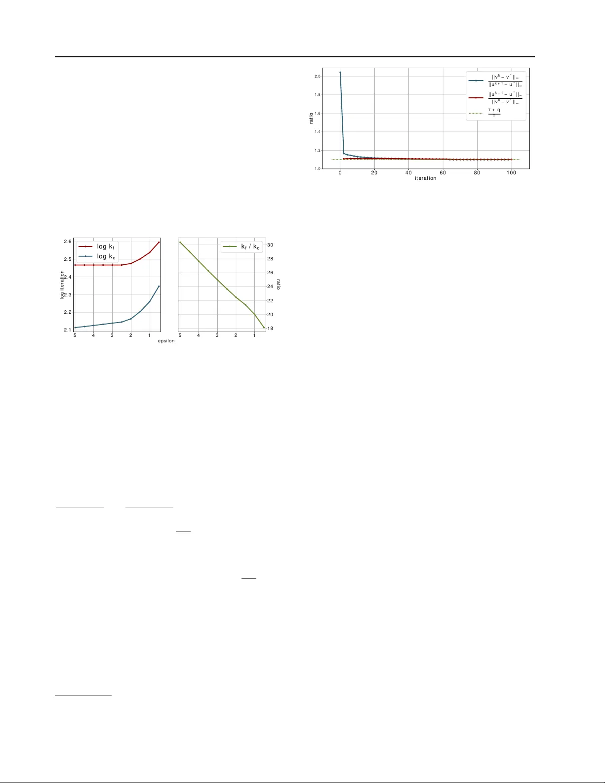
On Unbalanced Optimal T ransport: An Analysis of Sinkhorn Algorithm Khiem Pham * 1 Khang Le * 1 Nhat Ho 2 T ung Pham 1 3 Hung Bui 1 Abstract W e provide a computational comple xity analysis for the Sinkhorn algorithm that solves the entropic regularized Unbalanced Optimal T ransport (UO T) problem between two measures of possibly dif fer- ent masses with at most n components. W e show that the complexity of the Sinkhorn algorithm for finding an ε -approximate solution to the UO T problem is of order e O ( n 2 /ε ) . T o the best of our knowledge, this comple xity is better than the best known complexity upper bound of the Sinkhorn algorithm for solving the Optimal Transport (O T) problem, which is of order e O ( n 2 /ε 2 ) . Our proof technique is based on the geometric con ver gence rate of the Sinkhorn updates to the optimal dual solution of the entropic regularized UO T problem and scaling properties of the primal solution. It is also dif ferent from the proof technique used to establish the complexity of the Sinkhorn algo- rithm for approximating the O T problem since the UO T solution does not need to meet the marginal constraints of the measures. 1. Introduction The Optimal T ransport (O T) problem has a long history in mathematics and operation research, originally used to find the optimal cost to transport masses from one distri- bution to the other distribution ( V illani , 2003 ). Over the last decade, O T has emer ged as one of the most important tools to solve interesting practical problems in statistics and machine learning ( Ho et al. , 2017 ; Arjovsky et al. , 2017 ; Courty et al. , 2017 ; Sri vasta v a et al. , 2018 ; Peyr ´ e & Cuturi , 2019 ). Recently , the Unbalanced Optimal Transport (UO T) problem between tw o measures of possibly dif ferent masses has been used in sev eral applications in computational biol- * Equal contribution 1 V inAI Research 2 Department of EECS, Univ ersity of California, Berkele y 3 Faculty of Mathematics, Me- chanics and Informatics, Hanoi Univ ersity of Science, V ietnam National Univ ersity . Correspondence to: Nhat Ho < minhn- hat@berkeley .edu > . Pr oceedings of the 37 th International Conference on Machine Learning , Online, PMLR 119, 2020. Copyright 2020 by the au- thor(s). ogy ( Schiebinger et al. , 2019 ), computational imaging ( Lee et al. , 2019 ), deep learning ( Y ang & Uhler , 2019 ) and ma- chine learning and statistics ( Frogner et al. , 2015 ; Janati et al. , 2019a ). The UO T problem is a re gularized version of Kantorovich formulation which places penalty functions on the marginal distributions based on some gi ven di ver gences ( Liero et al. , 2018 ). When the two measures are the probability distribu- tions, the standard O T is a limiting case of the UO T . Under the discrete setting of the O T problem where each probabil- ity distribution has at most n components, the O T problem can be recast as a linear programming problem. The bench- mark methods for solving the OT problem are interior -point methods of which the most practical complexity is e O ( n 3 ) dev eloped by ( Pele & W erman , 2009 ). Recently , ( Lee & Sid- ford , 2014 ) used Laplacian linear system algorithms to im- prov e the complexity of interior -point methods to e O ( n 5 / 2 ) . Howe v er , the interior -point methods are not scalable when n is large. In order to deal with the scalability of computing the O T , ( Cuturi , 2013 ) proposed to regularize its objective func- tion by the entropy of the transportation plan, which results in the entropic regularized O T . One of the most popular algorithms for solving the entropic regularized O T is the Sinkhorn algorithm ( Sinkhorn , 1974 ), which was shown by ( Altschuler et al. , 2017 ) to ha ve a comple xity of e O ( n 2 /ε 3 ) when used to approximate the O T within an ε -accuracy . In the same article, ( Altschuler et al. , 2017 ) developed a greedy version of the Sinkhorn algorithm, named the Greenkhorn algorithm, that has a better practical perfor- mance than the Sinkhorn algorithm. Later , the complexity of the Greenkhorn algorithm was improv ed to e O ( n 2 /ε 2 ) by a deeper analysis in ( Lin et al. , 2019b ). In order to accelerate the Sinkhorn and Greenkhorn algorithms, ( Lin et al. , 2019a ) introduced Randkhorn and Gandkhorn algorithms that hav e complexity upper bounds of O ( n 7 / 3 /ε 4 / 3 ) . These com- plexities are better than those of Sinkhorn and Greenkhorn algorithms in terms of the desired accuracy ε . A different line of algorithms for solving the O T problem is based on primal-dual algorithms. These algorithms include acceler- ated primal-dual gradient descent algorithm ( Dvurechensky et al. , 2018 ), accelerated primal-dual mirror descent algo- rithm ( Lin et al. , 2019b ), and accelerated primal-dual coordi- nate descent algorithm ( Guo et al. , 2019 ). These primal-dual On Unbalanced Optimal T ransport: An Analysis of Sinkhorn Algorithm algorithms all hav e complexity upper bounds of e O ( n 2 . 5 /ε ) , which are better than those of Sinkhorn and Greenkhorn algorithms in terms of ε . Recently , ( Jamb ulapati et al. , 2019 ; Blanchet et al. , 2018 ) de v eloped algorithms with complexity upper bounds of e O ( n 2 /ε ) , which are belie ved to be optimal, based on either a dual extrapolation framework with area- con ve x mirror mapping or some black-box and specialized graph algorithms. Howe ver , these algorithms are quite diffi- cult to implement. Therefore, they are less competitiv e than Sinkhorn and Greenkhorn algorithms in practice. Our Contrib ution. While the comple xity theory for O T has been rather well-understood, that for UO T is still nascent. In the paper , we establish the complexity of approximating UO T between two discrete measures with at most n compo- nents. W e focus on the setting when the penalty functions are Kullback-Leiber (KL) di ver gences. Similar to the en- tropic regularized O T , in order to account for the scalability of computing UO T , we also consider an entropic version of UOT , which we refer to as entr opic r e gularized UOT . The Sinkhorn algorithm is widely used to solve the entropic regularized UO T ( Chizat et al. , 2016 ); ho we ver , its comple x- ity for approximating the UO T has not been studied. Our contribution is to prove that the Sinkhorn algorithm has a complexity of O  τ ( α + β ) n 2 ε log( n )  log( k C k ∞ ) + log(log( n )) + log  1 ε  , where C is a giv en cost matrix, α, β are total masses of the measures, and τ is a regularization parameter with the KL div er gences in the UO T problem. This complexity is close to the probably optimal one by a factor of logarithm of n and 1 /ε . The main dif ference between finding an ε -approximation solution for O T and UO T by the Sinkhorn algorithm is that the Sinkhorn algorithm for O T knows when it is close to the solution because of the constraints on the marginals, while the UO T does not hav e that advantage. Despite lacking that useful property , the Sinkhorn algorithm for UO T enjoys more freedom in its updates resulting in some interesting equations that relate the optimal v alue of the primal objec- tiv e function of UO T to the masses of two measures (see Lemma 4 ). Those equations together with the geometric con ver gence rate of the dual solution of the UO T pro ve the almost optimal con ver gence of Sinkhorn algorithm to an ε -approximation solution of the UO T . Organization. The remainder of the paper is or ganized as follows. In Section 2 , we provide a setup for the regular - ized UO T with KL diver gences in primal and dual forms, respectiv ely . Based on the dual form, we show that the dual solution has a geometric conv ergence rate in Section 3 . W e also sho w in Section 3 that the Sinkhorn algorithm for the UOT has a complexity of order ˜ O ( n 2 /ε ) . Section 4 presents some empirical results confirming the comple xity of the Sinkhorn algorithm. Finally , we conclude in Sec- tion 5 while deferring the proofs of remaining results in the supplementary material. Notation. W e let [ n ] stand for the set { 1 , 2 , . . . , n } while R n + stands for the set of all vectors in R n with nonnega- tiv e components for any n ≥ 2 . For a vector x ∈ R n and 1 ≤ p ≤ ∞ , we denote k x k p as its ` p -norm and diag ( x ) as the diagonal matrix with x on the diagonal. The natu- ral logarithm of a v ector a = ( a 1 , ..., a n ) ∈ R n is denoted log a = (log a 1 , ..., log a n ) . 1 n stands for a vector of length n with all of its components equal to 1 . ∂ x f refers to a par- tial gradient of f with respect to x . Lastly , given the dimen- sion n and accuracy ε , the notation a = O ( b ( n, ε )) stands for the upper bound a ≤ C · b ( n, ε ) where C is independent of n and ε . Similarly , the notation a = e O ( b ( n, ε )) indi- cates the previous inequality may depend on the logarithmic function of n and ε , and where C > 0 . 2. Unbalanced Optimal T ransport with Entropic Regularization In this section, we present the primal and dual forms of the entropic regularized UOT problem and define an ε - approximation for the solution of the unregularized UO T . For any two positiv e vectors a = ( a 1 , . . . , a n ) ∈ R n + and b = ( b 1 , . . . , b n ) ∈ R n + , the UO T problem tak es the form min X ∈ R n × n + f ( X ) where f ( X ) := h C , X i + τ KL ( X 1 n || a ) (1) + τ KL ( X > 1 n || b ) . Here, C is a given cost matrix, X is a transportation plan, τ > 0 is a given regularization parameter , and the KL div er gence between vectors x and y is defined as KL ( x k y ) := n X i =1 x i log  x i y i  − x i + y i . When a > 1 n = b > 1 n and τ → ∞ , the UO T problem be- comes the standard O T problem. Similar to the original O T problem, the exact computation of UO T is expensi v e and not scalable in terms of the number of supports n . Inspired by the recent success of the entropic re gularized O T problem as an efficient approximation of the O T problem, we also consider the entropic version of the UO T problem ( Frogner et al. , 2015 ) , which we refer to as entropic regularized UO T , of finding min X ∈ R n × n + g ( X ) , where g ( X ) := h C, X i − η H ( X ) + τ KL ( X 1 n || a ) + τ KL ( X > 1 n || b ) . (2) On Unbalanced Optimal T ransport: An Analysis of Sinkhorn Algorithm Here, η > 0 is a gi ven re gularization parameter and H ( X ) is an entropic regularization gi ven by H ( X ) := − n X i,j =1 X ij (log( X ij ) − 1) . (3) For each η > 0 , we can check that the entropic re gularized UO T problem is strongly conv ex in X . Therefore, it is con venient to solve for the optimal solution of the entropic regularized UO T and uses it to approximate the original value of UO T . Definition 1. F or any ε > 0 , we call X an ε -appr oximation transportation plan if the following holds h C, X i + τ KL ( X 1 n || a ) + τ KL ( X > 1 n || b ) ≤ D C, b X E + τ KL ( b X 1 n || a ) + KL ( b X > 1 n || b ) + ε, wher e b X is an optimal transportation plan for the UOT pr oblem ( 1 ) . W e aim to de velop an algorithm to obtain ε -approximation transportation plan for the UO T problem ( 1 ) . In order to do that, we consider the Fenchel-Legendre dual form of the entropic regularized UO T , which is gi ven by max u,v ∈ R n − F ∗ ( − u ) − G ∗ ( − v ) − η X i,j exp  u i + v j − C ij η  , where the functions F ∗ ( . ) and G ∗ ( . ) take the following forms: F ∗ ( u ) = max z ∈ R n z > u − τ KL ( z || a ) = τ D e u/τ , a E − a > 1 n , G ∗ ( v ) = max x ∈ R n x > v − τ KL ( x || b ) = τ D e v/τ , b E − b > 1 n . Since a and b are given non-negati ve vectors, finding the optimal solution for the abov e objectiv e is equiv alent to finding the optimal solution for the following objecti v e min u,v ∈ R n h ( u, v ) := η n X i,j =1 exp  u i + v j − C ij η  + τ D e − u/τ , a E + τ D e − v/τ , b E . (4) Problem ( 4 ) is referred to as the dual entr opic re gularized UO T . 3. Complexity Analysis of A pproximating Unbalanced Optimal T ransport In this section, we provide a complexity analysis of the Sinkhorn algorithm for approximating UOT solution. W e start with some notations and useful quantities followed by the lemmas and main theorems. 3.1. Notations and Assumptions W e first denote P n i =1 a i = α , P n j =1 b j = β . For each u, v ∈ R n , its corresponding optimal transport in the dual form ( 4 ) is denoted by B ( u, v ) , where B ( u, v ) := diag ( e u/η ) e − C η diag ( e v /η ) . The corresponding solution in ( 2 ) is denoted by X = B ( u, v ) . Let a = B ( u, v ) 1 n , b = B ( u, v ) > 1 n and P n i,j =1 X ij = x . Let ( u k , v k ) be the solution returned at the k -th iteration of the Sinkhorn algorithm and ( u ∗ , v ∗ ) be the optimal so- lution of ( 4 ) . Follo wing the above scheme, we also define X k , a k , b k , x k and X ∗ , a ∗ , b ∗ , x ∗ correspondingly . Ad- ditionally , we define b X to be the optimal solution of the unregularized objecti ve ( 1 ) and P n i,j =1 b X ij = b x . Different from the standard O T problem, the optimal solu- tions of the entropic regularized UO T and our complexity analysis ov erall also depend on the masses α, β and the KL regularization parameter τ . Gi ven that, we will assume the follo wing simple and standard re gularity conditions through- out the paper . Regularity Conditions: (A1) α , β , τ are positi ve constants. (A2) C is a matrix of non-negativ e entries. Before presenting the main theorem and analysis, we define some quantities that will be used in our analysis and quantify their magnitudes under the abov e regularity conditions. List of Quantities: R = max n k log( a ) k ∞ , k log( b ) k ∞ o + max  log( n ) , 1 η k C k ∞ − log( n )  , (5) ∆ k = max n k u k − u ∗ k ∞ , k v k − v ∗ k ∞ o , (6) Λ k = τ  τ τ + η  k R. (7) S = 1 2 ( α + β ) + 1 2 + 1 4 log( n ) , (8) T =  α + β 2   log  α + β 2  + 2 log( n ) − 1  + log( n ) + 5 2 , (9) U = max n S + T , 2 ε, 4 ε log( n ) τ , 4 ε ( α + β ) log ( n ) τ o . (10) As we shall see, the quantities ∆ k and Λ k are used to es- tablish the con v ergence rate of ( u k , v k ) . W e now consider the order of R, S and T . Since the order of the penalty function η H ( X ) is O ( η log( n )) and should be small for a good approximation, η is often chosen such that η log( n ) is sufficiently small (see our choice of η = ε U in Theorem 2 ). On Unbalanced Optimal T ransport: An Analysis of Sinkhorn Algorithm Algorithm 1 UNB ALANCED SINKHORN ( C , ε ) Input: k = 0 and u 0 = v 0 = 0 and η = ε/U while k ≤  τ U ε + 1 h log(8 η R  + log( τ ( τ + 1)) + 3 log( U ε ) i do a k = B ( u k , v k ) 1 n . b k = B ( u k , v k ) > 1 n . if k is ev en then u k +1 =  u k η + log ( a ) − log  a k   η τ η + τ v k +1 = v k else v k +1 =  v k η + log ( b ) − log  b k   η τ η + τ u k +1 = u k . end if k = k + 1 . end while Output: B ( u k , v k ) . Therefore, we can assume the dominant factor in the second term of R is 1 η k C k ∞ . If α = P n i =1 a i is a positiv e con- stant, then we can e xpect that a i is as small as O ( n − κ ) for a constant κ ≥ 1 . In this case, k log ( a ) k ∞ = O (log ( n )) . Overall, we can assume that R = O  1 η k C k ∞  and if α, β and τ are positiv e constants, then S = O  1  and T = O  log( n )  . 3.2. Sinkhorn Algorithm The Sinkhorn algorithm ( Chizat et al. , 2016 ) alternatively minimizes the dual function in ( 4 ) with respect to u and v . Suppose we are at iteration k + 1 for k ≥ 0 and k ev en, by setting the gradient to 0 we can see that gi ven fixed v k , the update u k +1 that minimizes the function in ( 4 ) satisfies exp u k +1 i η ! n X j =1 exp v k j − C ij η ! = exp − u k +1 i τ ! a i . Multiplying both sides by exp  u k i η  , we get: exp  u k +1 i η  a k i = exp  u k i η  exp − u k +1 i τ ! a i . Similarly with u k fixed and k is odd: exp  v k +1 j η  b k j = exp v k j η ! exp − v k +1 j τ ! b j . These equations translate to the pseudocode of Algorithm 1 , in which we hav e included our stopping condition stated in Theorem 2 . W e now present the main theorems. Theorem 1. F or any k ≥ 0 , the update ( u k +1 , v k +1 ) fr om Algorithm 1 satisfies the following bound ∆ k +1 ≤ Λ k , (11) wher e ∆ k and Λ k ar e defined in ( 6 ) and ( 7 ) , respectively . Remark 1. Theor em 1 establishes a geometric con ver gence rate for the dual solution ( u k , v k ) under ` ∞ norm. Its ge- ometric con ver gence is similar to the work of ( S ´ ejourn ´ e et al. , 2019 ) while it is differ ent fr om the work of ( Chizat et al. , 2016 ), whic h used the Thompson metric. The differ - ence between the r esult of Theor em 1 and that in ( S ´ ejourn ´ e et al. , 2019 ) is that we obtain a specific upper bound for the con ver gence rate of the Sinkhorn updates, which depends explicitly on the number of components n and all other pa- rameters of masses and penalty functions. The con ver gence rate of Theor em 1 plays an important r ole in the complexity analysis of the Sinkhorn algorithm in the next theor em. Theorem 2. Under the r e gularity conditions (A1-A2), with R and U defined in ( 5 ) and ( 10 ) r espectively , for η = ε U and k ≥ 1 +  τ U ε + 1  log(8 η R  + log ( τ ( τ + 1)) + 3 log( U ε )  , the update X k fr om Algorithm 1 is an ε -appr oximation of the optimal solution b X of ( 1 ) . The next corollary sums up the comple xity of Algorithm 1 . Corollary 1. Under conditions (A1-A2) and assume that R = O  1 η k C k ∞  , S = O (1) and T = O (log ( n )) . Then the complexity of Algorithm 1 is O  τ ( α + β ) n 2 ε log( n )  log( k C k ∞ ) + log(log( n )) + log  1 ε  . Pr oof of Cor ollary 1 . By the assumptions on the order of R, S , T , we hav e R = O ( 1 η k C k ∞ ) , S = O ( α + β ) , T = O (( α + β ) log( n )) . Plugging the abov e results into the definition of U in ( 10 ) , we find that U = O ( S ) + O ( T ) + ε O (log( n )) = O (( α + β ) log ( n )) . Overall, we obtain k = O  τ ( α + β ) log( n ) ε  log( k C k ∞ ) + log(log( n )) + log  1 ε  . By multiplying the abov e bound of k with O ( n 2 ) arithmetic operations per iteration, we obtain the desired final com- plexity of the Sinkhorn algorithm as being claimed in the conclusion of the corollary . On Unbalanced Optimal T ransport: An Analysis of Sinkhorn Algorithm Remark 2. Since α , β and τ ar e positive constants, we obtain the complexity e O  n 2 /  as stated in the abstract. In comparison to the best known OT’ s complexity of the similar order of n , i.e., ( Dvurec hensky et al. , 2018 ; Lin et al. , 2019b ), our complexity for the UOT is better by a factor of ε . Meanwhile, among the practical algorithms for OT which have complexity of the or der of n 7 / 3 , i.e., Gankhorn and Randkhorn algorithms ( Lin et al. , 2019a ), our bound is better by a factor of n 1 / 3 . 3.3. Proof of Theor em 1 The analysis of Sinkhorn algorithm for approximating un- balanced optimal transport is dif ferent from that of optimal transport, since a and b need not be probability measures. Our proof of Theorem 1 requires the geometric con ver gence rate of ( u k , v k ) and an upper bound on the supremum norm of the optimal dual solution ( u ∗ , v ∗ ) . The latter result is presented in Lemma 3 . Before stating that result formally , we need the following lemmas. Lemma 1. The optimal solution ( u ∗ , v ∗ ) of dual entr opic r e gularized UO T ( 4 ) satisfies the following equations: u ∗ τ = log( a ) − log( a ∗ ) , and v ∗ τ = log( b ) − log( b ∗ ) . Pr oof. Since ( u ∗ , v ∗ ) is a fixed point of the updates in the Algorithm 1 , we get u ∗ =  u ∗ η + log ( a ) − log( a ∗ )  η τ η + τ . This directly leads to the stated equality for u ∗ , and that for v ∗ can be obtained similarly . Lemma 2. Assume that the r e gularity conditions (A1-A2) hold. Then, the following ar e true: ( a )    log  a ∗ i a k i  − u ∗ i − u k i η    ≤ max 1 ≤ j ≤ n | v ∗ j − v k j | η , ( b )    log b ∗ j b k j ! − v ∗ j − v k j η    ≤ max 1 ≤ i ≤ n | u ∗ i − u k i | η . The proof is giv en in the supplementary material. Lemma 3. The sup norms of the optimal solution k u ∗ k ∞ and k v ∗ k ∞ ar e bounded by: max {k u ∗ k ∞ , k v ∗ k ∞ } ≤ τ R, wher e R is defined in equation ( 5 ) . Pr oof. W e start with the equations for the solution u ∗ in Lemma 1 , i.e., we hav e u ∗ i τ = log( a i ) − log   n X j =1 exp  u ∗ i + v ∗ j − C ij η    , which can be rewritten as u ∗ i  1 τ + 1 η  = log( a i ) − log   n X j =1 exp  v ∗ j − C ij η    . The second term in the abov e display can be lower bounded as follows log " n X j =1 exp  v ∗ j − C ij η  # ≥ log( n ) + min 1 ≤ j ≤ n  v ∗ j − C ij η  ≥ log( n ) − k v ∗ k ∞ η − k C k ∞ η . Additionally , we also have log " n X j =1 exp  v ∗ j − C ij η  # ≤ log( n ) + max 1 ≤ j ≤ n  v ∗ j − C ij η  ≤ log( n ) + k v ∗ k ∞ η . Collecting the abov e results, we find that       log   n X j =1 exp  v ∗ j − C ij η          ≤ k v ∗ k ∞ η + max  log( n ) , k C ∗ k ∞ η − log ( n )  . Hence, we obtain that | u ∗ i |  1 τ + 1 η  ≤ | log ( a i ) | + k v ∗ k ∞ η + max  log( n ) , k C ∗ k ∞ η − log ( n )  . By choosing an index i such that | u ∗ i | = k u ∗ k ∞ and combining with the fact that | log ( a i ) | ≤ max {k log( a ) k ∞ , k log ( b ) k ∞ } , we hav e k u ∗ k ∞  1 τ + 1 η  ≤ k v ∗ k ∞ η + R. WLOG assume that k u ∗ k ∞ ≥ k v ∗ k ∞ . Then, we obtain the stated bound in the conclusion. Proof of Theor em 1 W e first consider the case when k is ev en. From the update of u k +1 in Algorithm 1 , we hav e: u k +1 i =  u k i η + log a i − log a k i  η τ τ + η =  u k i η + [log( a i ) − log( a ∗ i )] + h log( a ∗ i ) − log( a k i ) i  η τ τ + η . On Unbalanced Optimal T ransport: An Analysis of Sinkhorn Algorithm Using Lemma 1 , the abov e equality is equiv alent to u k +1 i − u ∗ i =  η log  a ∗ i a k i  − ( u ∗ i − u k i )  τ τ + η . Using Lemma 2 , we get   u k +1 i − u ∗ i   ≤ max 1 ≤ j ≤ n   v k j − v ∗ j   τ τ + η . This leads to k u k +1 − u ∗ k ∞ ≤ τ τ + η k v k − v ∗ k ∞ . Similarly , we obtain k v k − v ∗ k ∞ ≤ τ τ + η k u k − 1 − u ∗ k ∞ . Combining the two inequalities yields k u k +1 − u ∗ k ∞ ≤  τ τ + η  2 k u k − 1 − u ∗ k ∞ . Repeating all the abov e arguments alternati vely , we have k u k +1 − u ∗ k ∞ ≤  τ τ + η  k +1 k v 0 − v ∗ k ∞ =  τ τ + η  k +1 k v ∗ k ∞ . Note that v k +1 = v k for k ev en. Therefore, we find that k v k +1 − v ∗ k ∞ ≤ τ τ + η k u k − 1 − u ∗ k ∞ ≤  τ τ + η  k k v ∗ k ∞ . These two results lead to ∆ k +1 ≤  τ τ + η  k k v ∗ k ∞ . Simi- larly , for k odd we obtain ∆ k +1 ≤  τ τ + η  k k v ∗ k ∞ . Thus the abov e inequality is true for all k . Using the fact that k v ∗ k ∞ ≤ max {k u ∗ k ∞ , k v ∗ k ∞ } and Lemma 3 , we obtain the conclusion of Theorem 1 . 3.4. Proof of Theor em 2 The proof is based on the upper bound for the con ver gence rate in Theorem 1 and an upper bound for the solutions b x and x ∗ of functions in equations ( 1 ) and ( 2 ) , respectively , which are direct consequences of the following lemmas. Lemma 4. Assume that the function g attains its minimum at X ∗ , then g ( X ∗ ) + (2 τ + η ) x ∗ = τ ( α + β ) . (12) Similarly , assume that f attains its minimum at b X , then f ( b X ) + 2 τ b x = τ ( α + β ) , (13) wher e P n i,j =1 X ∗ = x ∗ and P n i,j =1 b X = b x . Both equations in Lemma 4 establish the relationships be- tween the optimal solutions of functions in equations ( 1 ) and ( 2 ) with other parameters. Those relationships are very useful for analysing the behaviour of the optimal solution of UO T , because the UOT does not ha ve an y conditions on the marginals as the O T does. Consequences of Lemma 4 include Corollary 2 which provides the upper bounds for b x and x ∗ as well as bounds for the entropic functions in the proof of Theorem 2 . The key idea of the proof surprisingly comes from the fact that the UO T solution does not have to meet the marginal constraints. W e note that equation ( 12 ) could also be prov ed by using the fixed point equations in Lemma 1 as in ( Janati et al. , 2019b ). Here we offer an alternativ e proof that can be applied to the unregularized case as well. W e now present the proof of Lemma 4 . Pr oof. Consider the function g ( tX ∗ ) , where t ∈ R + , g ( tX ∗ ) = h C, tX ∗ i + τ KL ( tX ∗ 1 n k a ) + τ KL (( tX ∗ ) > 1 n k b ) − ηH ( tX ∗ ) . For the KL term of g ( tX ∗ ) , we hav e: KL ( tX ∗ 1 n k a ) = n X i =1 ( ta ∗ i ) log  ta ∗ i a i  − n X i =1 ( ta ∗ i ) + n X i =1 a i = n X i =1 ( ta ∗ i )  log  a ∗ i a i  + log ( t )  − tx ∗ + α = t n X i =1  a ∗ i log  a ∗ i a i  − x ∗ + a i  + (1 − t ) α + x ∗ t log ( t ) = t KL ( X ∗ 1 n k a ) + (1 − t ) α + x ∗ t log ( t ) . Similarly , we get KL ( t ( X ∗ ) > 1 n k b ) = t KL  ( X ∗ ) > 1 n k b  + (1 − t ) β + x ∗ t log ( t ) . For the entropic penalty term, we find that − H ( tX ∗ ) = n X i,j =1 tX ∗ ij  log( tX ∗ ij ) − 1  = X i,j tX ∗ ij  log( X ∗ ij ) − 1  + x ∗ t log ( t ) = − tH ( X ∗ ) + x ∗ t log ( t ) . Putting all results together , we obtain g ( tX ∗ ) = tg ( X ∗ ) + τ (1 − t )( α + β ) + (2 τ + η ) x ∗ t log ( t ) . On Unbalanced Optimal T ransport: An Analysis of Sinkhorn Algorithm T aking the deriv ati v e of g ( tX ∗ ) with respect to t , ∂ g ( tX ∗ ) ∂ t = g ( X ∗ ) − τ ( α + β ) + (2 τ + η ) x ∗ (1 + log( t )) . The function g ( tX ∗ ) is well-defined for all t ∈ R + . W e know that g ( tX ∗ ) attains its minimum at t = 1 . Replace t = 1 into the abov e equation, we obtain g ( X ∗ ) − τ ( α + β ) + (2 τ + η ) x ∗ = 0 g ( X ∗ ) + (2 τ + η ) x ∗ = τ ( α + β ) . The second claim is prov ed in the same way . Corollary 2. Assume that conditions (A1-A2) hold and η log( n ) is sufficiently small. W e have the following bounds on x ∗ and b x : ( a ) x ∗ ≤  1 2 + η log( n ) 2 τ − 2 η log ( n )  ( α + β ) + 1 6 log ( n ) , ( b ) b x ≤ α + β 2 . W e defer the proof of Corollary 2 to the appendix. Next, we use the condition for k in Theorem 2 to bound some relev ant quantities at the k -th iteration of the Sinkhorn algorithm. Lemma 5. Assume that the r e gularity conditions (A1-A2) hold and k satisfies the inequality in Theor em 2 . The follow- ing ar e true ( a ) Λ k − 1 ≤ η 2 8( τ + 1) , ( b ) | x k − x ∗ | ≤ 3 η ∆ k min  x ∗ , x k  , ( c ) x k ≤ S, wher e S is defined in equation ( 8 ) . W e are now ready to construct a proof for Theorem 2 . Proof of Theor em 2 From the definitions of f and g , we hav e f ( X k ) − f ( b X ) = g ( X k ) + η H ( X k ) − g ( b X ) − η H ( b X ) = g ( X k ) + η H ( X k ) − g ( b X ) − η H ( b X ) − g ( X ∗ ) + g ( X ∗ ) ≤ h g ( X k ) − g ( X ∗ ) i + η h H ( X k ) − H ( b X ) i , (14) since g ( X ∗ ) − g ( b X ) ≤ 0 , as X ∗ is the optimal solution of function ( 2 ) . The abov e two terms can be bounded sepa- rately as follows: Upper Bound of H ( X k ) − H ( b X ) . W e first show the follo wing inequalities x − x log( x ) ≤ H ( X ) ≤ 2 x log( n ) + x − x log ( x ) (15) for any X that X ij ≥ 0 and x = P ij X ij . Indeed, rewriting − H ( X ) as − H ( X ) = x h n X i,j =1 X ij x log  X ij x  − 1 i + x log( x ) , and using − 2 log ( n ) ≤ P n i,j =1 X ij x log  X ij x  ≤ 0 , we thus obtain equation ( 15 ). Now apply the lo wer bound of ( 15 ) to − H ( b X ) − H ( b X ) ≤ b x log ( b x ) − b x ≤ max  0 , α + β 2  log( α + β 2 ) − 1  ≤ α + β 2 log( α + β 2 ) − α + β 2 + 1 , where the second inequality is due to x log x − x being con ve x and 0 ≤ b x ≤ 1 2 ( α + β ) by Corollary 2 and the third inequality is due to α + β 2  log( α + β 2 ) − 1  + 1 ≥ 0 . Similarly , apply the upper bound of equation ( 15 ) to H ( X k ) H ( X k ) ≤ 2 x k log( n ) + x k − x k log( x k ) ≤ 2 x k log( n ) + 1 ≤  α + β + 1 + 1 2 log ( n )  log( n ) + 1 , where the last inequality is due to Lemma 5 (c). By combin- ing the two results, we ha ve H ( X k ) − H ( b X ) ≤ T , (16) where T is defined in equation ( 9 ). Upper Bound of g ( X k ) − g ( X ∗ ) . WLOG we assume that k is odd. At step k − 1 of Algorithm 1 , we find u k by minimizing the dual function ( 4 ) giv en a and fixed v k − 1 , and simply keep v k = v k − 1 . Hence, X k = B ( u k , v k ) is the optimal solution of min X ∈ R n × n + g k ( X ) := h C , X i − ηH ( X ) + τ KL ( X 1 n || a ) + τ KL ( X > 1 n || b k ) , where b k = exp  v k τ    ( X k ) T 1 n  with  denoting element-wise multiplication. Denote P n i =1 b k i = β k . By Lemma 4 , g k ( X k ) = τ  α + β k  − (2 τ + η ) x k , g ( X ∗ ) = τ  α + β  − (2 τ + η ) x ∗ . On Unbalanced Optimal T ransport: An Analysis of Sinkhorn Algorithm Writing g ( X k ) − g ( X ∗ ) =  g ( X k ) − g k ( X k )  +  g k ( X k ) − g ( X ∗ )  , following some deri vations using the abov e equations of g k ( X k ) and g ( X ∗ ) and the definitions of g ( X k ) and g k ( X k ) , we get g ( X k ) − g ( X ∗ ) = h − (2 τ + η )( x k − x ∗ ) i + τ " n X j =1 b k j log b k j b j !# . (17) By part (b) of Lemma 5 , the first term is bounded by (2 τ + η ) 3 η ∆ k x k . Note that b k j = exp  v k j τ  b k j and b j = exp  v ∗ j τ  b ∗ j . Use part (b) of Lemma 2 , we find that log b k j b j ! = " − log b ∗ j b k j !# + 1 τ ( v k j − v ∗ j ) ,      log b k j b j !      ≤  2 η ∆ k  +  1 τ ∆ k  =  2 η + 1 τ  ∆ k . Note that b k j ≥ 0 for all j . The abov e inequality leads to       n X j =1 b k j log b k j b j !       ≤   n X j =1 b k j   max 1 ≤ j ≤ n      log b k j b j !      ≤ x k  2 η + 1 τ  ∆ k . W e hav e g ( X k ) − g ( X ∗ ) ≤ [(2 τ + η ) + 3(2 τ + η )]  ∆ k η  x k ≤ 8( τ + 1)  Λ k − 1 η  S, where the first inequality is obtained by combining the bounds for two terms of ( 17 ) while the second inequality results from the fact that η = ε U ≤ ε 2 ε = 1 2 with U defined in ( 10 ), part ( c ) of Lemma 5 , and Theorem 1 . Using part ( a ) of Lemma 5 , this leads to g ( X k ) − g ( X ∗ ) ≤ η S. (18) Combining ( 14 ) , ( 16 ) , ( 18 ) and the fa ct that η = ε U ≤ ε S + T , we get f ( X k ) − f ( b X ) ≤ η S + η T ≤ ε. As a consequence, we obtain the conclusion of Theorem 2 . 4. Experiments In this section, we pro vide empirical e vidence to illustrate our prov en complexity on both synthetic data and real im- ages. In both examples, we vary ε such that it is small relativ e to the minimum v alue of the unregularized UOT function in equation ( 1 ) which is computed in advance by using the cvxpy library ( Agraw al et al. , 2018 ) with the split- ting conic solver option. W e then report the two k values: • The first k , denoted by k f , follows the stopping rule in Algorithm 1 . • The second k , denoted by k c , is defined as the minimal k c such that for all later known iterations k 0 ≥ k c in the experiment, Algorithm 1 returns an ε -approximation solution of the UO T problem. 4.1. Synthetic Data For the simulated e xample, we choose n = 100 and τ = 5 . The elements of the cost matrix C are drawn uniformly from the closed interval [1 , 50] while those of the marginal vectors a and b are drawn uniformly from [0 . 1 , 1] and then normalized to ha ve masses 2 and 4 , respecti v ely . By v arying ε from 1 . 0 to 10 − 4 (here we uniformly vary log( 1 ε ) in the corresponding range for visualization purpose), we follo w the scheme presented in the beginning of the section, and report values of k f and k c in Figure 1 . 0 2 4 6 8 6 8 1 0 1 2 1 4 1 6 1 8 l o g i t e r a t i o n l o g k f l o g k c 0 2 4 6 8 1 0 1 2 1 4 1 6 1 8 r a t i o k f / k c l o g ( 1 / e p s i l o n ) Figure 1. Comparison between k c and k f on the synthetic data when varying ε from 1 to 10 − 4 (and η from 3 . 7(10) − 2 to 3 . 7(10) − 6 as computed from Theorem 2 ). The optimal value here is f ( b X ) = 17 . 28 , yielding a relative error from 5 . 8(10) − 2 to 5 . 8(10) − 6 . Both x-axes represent log( 1 ε ); the y-axis of the left plot is the natural logarithm of the numbers of iteration (i.e. k f , k c ) and the y-axis of the right plot is the ratio between them. Figure 1 sho ws the log v alues of k f , k c stated abov e when varying ε . When ε becomes smaller , the left plot indicates that the gap between k f and k c becomes narrower , while the right plot sho ws that the ratio k f k c decreases ( k f k c ≈ 18 at ε = 1 , going down to about 8 at ε = 10 − 4 ). W e hypothesize from this trend that our bound becomes more and more accurate as ε approaches 0 . On Unbalanced Optimal T ransport: An Analysis of Sinkhorn Algorithm 4.2. MNIST Data For the MNIST dataset 1 , we follow similar settings in ( Dvurechensky et al. , 2018 ; Altschuler et al. , 2017 ). In particular , the mar ginals a , b are two flattened images in a pair and the cost matrix C is the matrix of ` 1 distances between pixel locations. W e also add a small constant 10 − 6 to each pix el with intensity 0, e xcept we do not normalize the marginals. W e average the results ov er 10 randomly chosen image pairs and plot the results in Figure 2 . The results on MNIST dataset confirm our theoretical results on the bound of k in Theorem 2 . It also shows that the smaller ε in the approximation, the closer the empirical result to the theoretical result. 1 2 3 4 5 2 . 1 2 . 2 2 . 3 2 . 4 2 . 5 2 . 6 l o g i t e r a t i o n l o g k f l o g k c 1 2 3 4 5 1 8 2 0 2 2 2 4 2 6 2 8 3 0 r a t i o k f / k c e p s i l o n Figure 2. Comparison between log( k f ) and log( k c ) on MNIST when varying ε from 5 to 0 . 5 . W e used higher ε to keep the relativ e error similar to the first e xperiment, due to a higher optimal value (among 10 chosen pairs, the minimum was 117 . 524 and the maximum was 459 . 297 .) 4.3. A Further Analysis for Synthetic Data In order to in v estigate ho w challenging it is to improv e the theoretical bound for the number of required iterations, we carry out a deeper analysis on the synthetic example. In particular , we set η = 0 . 5 , τ = 5 and compute the ratios k v k − v ∗ k ∞ k u k +1 − u ∗ k ∞ and k u k − 1 − u ∗ k ∞ k v k − v ∗ k ∞ for even k in range [0 , 100] and plot them in Figure 3 . As has been proved in Theorem 1 , these ratios are no less than τ + η τ . The main reason for this choice is that these differences are used to construct bounds for many key quantities in lemmas and theorems. These ratios, which are extremely close to 1 . 1 for most of the iterations, are consistent with the ratio τ + η τ = 1 . 1 . Consequently , it is difficult to improve our inequalities in Theorem 1 . 5. Discussion In this paper , we prove the near-optimal upper bound of order e O ( n 2 /ε ) of the complexity of the Sinkhorn algorithm for approximating the unbalanced optimal transport prob- lem. That complexity is better than the complexity of the 1 http://yann.lecun.com/exdb/mnist/ 0 2 0 4 0 6 0 8 0 1 0 0 i t e r a t i o n 1 . 0 1 . 2 1 . 4 1 . 6 1 . 8 2 . 0 r a t i o | | v k − v * | | ∞ | | u k + 1 − u * | | ∞ | | u k − 1 − u * | | ∞ | | v k − v * | | ∞ τ + η τ Figure 3. The ratios as observed empirically remain close to our geometric factor for most of the iterations. Sinkhorn algorithm for approximating the O T problem. In our analysis, some inequalities might not be tight, since we prefer to keep them in simple forms for easier presentation. These sub-optimalities perhaps lead to the inclusion of the logarithmic terms of ε and n in our comple xity upper bound of the Sinkhorn algorithm. W e now discuss a few future directions that can serve as natural follo w-ups of our w ork. First, our analysis could be used in the multi-marginal case of UO T by applying Algorithm 1 repeatedly to every pair of marginals. Second, since the UO T barycenter problem has found se veral applications in recent years ( Janati et al. , 2019a ; Schiebinger et al. , 2019 ), it is desirable to establish the complexity analysis of algorithms for approximating it. Finally , similar to the O T problem, the Sinkhorn algorithm for solving UO T also suffers from the curse of dimensional- ity , namely , when the supports of the measures lie in high dimensional spaces. An important direction is to study ef fi- cient dimension reduction scheme with the UO T problem and optimal algorithms for solving it. On Unbalanced Optimal T ransport: An Analysis of Sinkhorn Algorithm References Agrawal, A., V erschueren, R., Diamond, S., and Boyd, S. A rewriting system for con v ex optimization problems. Journal of Contr ol and Decision , 5(1):42–60, 2018. Altschuler , J., W eed, J., and Rigollet, P . Near-linear time ap- proximation algorithms for optimal transport via sinkhorn iteration. In Advances in Neural Information Pr ocessing Systems , pp. 1964–1974, 2017. Arjovsk y , M., Chintala, S., and Bottou, L. W asserstein gen- erativ e adversarial networks. In International confer ence on machine learning , pp. 214–223, 2017. Blanchet, J., Jambulapati, A., K ent, C., and Sidford, A. T o- wards optimal running times for optimal transport. ArXiv Pr eprint: 1810.07717 , 2018. Chizat, L., Peyr ´ e, G., Schmitzer , B., and V ialard, F . Scaling algorithms for unbalanced transport problems. ArXiv Pr eprint: 1607.05816 , 2016. Courty , N., Flamary , R., T uia, D., and Rakotomamonjy , A. Optimal transport for domain adaptation. IEEE T ransac- tions on P attern Analysis and Machine Intelligence , 39 (9):1853–1865, 2017. Cuturi, M. Sinkhorn distances: Lightspeed computation of optimal transport. In Advances in Neural Information Pr ocessing Systems , pp. 2292–2300, 2013. Dvurechensky , P ., Gasnikov , A., and Kroshnin, A. Com- putational optimal transport: Complexity by accelerated gradient descent is better than by Sinkhorn’ s algorithm. In International confer ence on machine learning , pp. 1367– 1376, 2018. Frogner , C., Zhang, C., Mobahi, H., Araya, M., and Poggio, T . A. Learning with a wasserstein loss. In Advances in Neural Information Pr ocessing Systems , pp. 2053–2061, 2015. Guo, W ., Ho, N., and Jordan, M. I. Accelerated primal-dual coordinate descent for computational optimal transport. ArXiv Pr eprint: 1905.09952 , 2019. Ho, N., Nguyen, X., Y urochkin, M., Bui, H., Huynh, V ., and Phung, D. Multilev el clustering via Wasserstein means. In Pr oceedings of the International Confer ence on Machine Learning , 2017. Jambulapati, A., Sidford, A., and T ian, K. A direct e O (1 /ε ) iteration parallel algorithm for optimal transport. ArXiv Pr eprint: 1906.00618 , 2019. Janati, H., Cuturi, M., and Gramfort, A. W asserstein regu- larization for sparse multi-task regression. In AIST A TS , 2019a. Janati, H., Cuturi, M., and Gramfort, A. Spatio-temporal alignments: Optimal transport through space and time. arXiv pr eprint arXiv:1910.03860 , 2019b. Lee, J., Bertrand, N. P ., and Rozell, C. J. Parallel unbalanced optimal transport regularization for large scale imaging problems. arXiv preprint , 2019. Lee, Y . T . and Sidford, A. Path finding methods for linear programming: Solving linear programs in e O ( √ r ank ) iterations and faster algorithms for maximum flow . In FOCS , pp. 424–433. IEEE, 2014. Liero, M., Mielke, A., and Sa v ar ´ e, M. I. Optimal entropy- transport problemsand a new Hellinger–Kantorovich dis- tance between positi ve measures. Inventiones Mathemati- cae , 211:969–1117, 2018. Lin, T ., Ho, N., and Jordan, M. I. On the acceleration of the Sinkhorn and Greenkhorn algorithms for optimal transport. ArXiv Preprint: 1906.01437 , 2019a. Lin, T ., Ho, N., and Jordan, M. I. On efficient optimal transport: An analysis of greedy and accelerated mirror descent algorithms. ArXiv Pr eprint: 1901.06482 , 2019b. Pele, O. and W erman, M. Fast and robust earth mover’ s distance. In ICCV . IEEE, 2009. Peyr ´ e, G. and Cuturi, M. Computational optimal transport. F oundations and T r ends ® in Machine Learning , 11(5-6): 355–607, 2019. Schiebinger , G. et al. Optimal-transport analysis of single- cell gene expression identifies dev elopmental trajectories in reprogramming. Cell , 176:928–943, 2019. S ´ ejourn ´ e, T ., Feydy , J., V ialard, F .-X., Trouv ´ e, A., and Peyr ´ e, G. Sinkhorn div ergences for unbalanced optimal transport. arXiv preprint , 2019. Sinkhorn, R. Diagonal equi valence to matrices with pre- scribed row and column sums. Pr oceedings of the Ameri- can Mathematical Society , 45(2):195–198, 1974. Sriv asta v a, S., Li, C., and Dunson, D. Scalable Bayes via barycenter in Wasserstein space. Journal of Machine Learning Resear ch , 19(8):1–35, 2018. V illani, C. T opics in Optimal T ransportation . American Mathematical Society , 2003. Y ang, K. D. and Uhler , C. Scalable unbalanced optimal transport using generativ e adversarial networks. In ICLR , 2019. Supplement to ”On Unbalanced Optimal T ransport: An Analysis of Sinkhorn Algorithm” In this appendix, we provide proofs for the remaining results in the paper . 6. Proofs of Remaining Results Before proceeding with the proofs, we state the following simple inequalities: Lemma 6. The following inequalities are true for all positive x i , y i , x , y and 0 ≤ z < 1 2 : ( a ) min 1 ≤ i ≤ n x i y i ≤ P n i =1 x i P n i =1 y i ≤ max 1 ≤ i ≤ n x i y i , ( b ) exp( z ) ≤ 1 + | z | + | z | 2 , ( c ) If max n x y , y x o ≤ 1 + δ , then | x − y | ≤ δ min { x, y } , ( d )  1 + 1 x  x +1 ≥ e. Pr oof of Lemma 6 . (a) Giv en x i and y i positiv e, we ha ve min 1 ≤ i ≤ n x i y i ≤ x j y j ≤ max 1 ≤ i ≤ n x i y i , y j  min 1 ≤ i ≤ n x i y i  ≤ x j ≤ y j  max 1 ≤ i ≤ n x i y i  . T aking the sum ov er j , we get   n X j =1 y j    min 1 ≤ i ≤ n x i y i  ≤ n X j =1 x j ≤   n X j =1 y j    max 1 ≤ i ≤ n x i y i y j  , min 1 ≤ i ≤ n x i y i ≤ P n j =1 x j P n j =1 y j ≤ max 1 ≤ i ≤ n x i y i . (b) For the second inequality , exp( x ) ≤ 1 + | x | + | x | 2 , we hav e to deal with the case x > 0 . Since x ≤ 1 2 , exp( x ) = ∞ X n =1 x n n ! = 1 + x + x 2 − x 2 2 + ∞ X n =3 x n n ! ≤ 1 + x + x 2 − x 2 2 + x 3 6 ∞ X n =3 x n − 3 , ≤ 1 + x + x 2 − x 2 2 + x 3 6 1 1 − x ≤ 1 + x + x 2 − x 2 2 + x 3 3 ≤ 1 + x + x 2 . (c) For the third inequality , WLOG assume x > y . Then, we hav e x y ≤ 1 + δ ⇒ x ≤ y + y δ ⇒ | x − y | ≤ y δ. (d) For the fourth inequality , taking the log of both sides, it is equi valent to ( x + 1)  log( x + 1) − log ( x )  ≥ 1 . By the mean val ue theorem, there exists a number y between x and x + 1 such that log( x + 1) − log( x ) = 1 /y , then ( x + 1) /y ≥ 1 . On Unbalanced Optimal T ransport: An Analysis of Sinkhorn Algorithm By the choice of η = ε U and the definition of U , we also have the follo wing conditions on η : η ≤ 1 2 ; η τ ≤ 1 4 log ( n ) max { 1 , α + β } . (19) Now we come to the proofs of lemmas and the corollary in the main te xt. 6.1. Proof of Lemma 2 (a) + (b) : From the definitions of a k i and a ∗ i , we hav e log  a ∗ i a k i  =  u ∗ i − u k i η  + log   P n j =1 exp( v ∗ j − C ij η ) P n j =1 exp( v k j − C ij η )   . The required inequalities are equi valent to an upper bound and a lo wer bound for the second term of the RHS. Apply part (a) of Lemma 6 , we obtain min 1 ≤ j ≤ n v ∗ j − v k j η ≤ log  a ∗ i a k i  − u ∗ i − u k i η ≤ max 1 ≤ j ≤ n v ∗ j − v k j η . Part (b) follo ws similarly . Therefore, we obtain the conclusion of Lemma 2 . 6.2. Proof of Cor ollary 2 Recall that we hav e prov ed in Lemma 4 : g ( X ∗ ) + (2 τ + η ) x ∗ = τ ( α + β ) , f ( b X ) + 2 τ b x = τ ( α + β ) . From the second equality and the fact that f ( b X ) ≥ 0 (it is easy to see that for X that X ij ≥ 0 , the KL terms and h C, X i are all non-negati ve), we immediately hav e b x ≤ α + β 2 , proving the second inequality . For the first inequality , we have g ( X ∗ ) ≥ − η H ( X ∗ ) ≥ − 2 η x ∗ log( n ) − η x ∗ + η x ∗ log( x ∗ ) . Therefore, we find that − 2 η x ∗ log( n ) − η x ∗ + η x ∗ log( x ∗ ) ≤ τ ( α + β ) − (2 τ + η ) x ∗ , η x ∗ log( x ∗ ) + 2  τ − η log ( n )  x ∗ ≤ τ ( α + β ) . It follows from the inequality z log ( z ) ≥ z − 1 for all z > 0 that η ( x ∗ − 1) + 2( τ − η log ( n )) x ∗ ≤ τ ( α + β ) , x ∗ (2 τ − 2 η log ( n ) + η ) ≤ τ ( α + β ) + η . By inequality ( 19 ), 4 η log( n ) ≤ τ . Then x ∗ ≤ τ ( α + β ) + η 2 τ − 2 η log ( n ) + η ≤ τ ( α + β ) − ( α + β ) η log( n ) 2 τ − 2 η log ( n ) + ( α + β ) η log( n ) + η 2 τ − 2 η log ( n ) , ≤ α + β 2 + ( α + β ) η log( n ) 2 τ − 2 η log ( n ) + τ 4 log ( n ) 3 2 τ ≤  1 2 + η log( n ) 2 τ − 2 η log ( n )  ( α + β ) + 1 6 log ( n ) . As a consequence, we obtain the conclusion of the corollary . 6.3. Proof of Lemma 5 (a) W e prov e that Λ k ≤ η 2 8( τ +1) for η = ε U and k ≥  τ η + 1  h log(8 η R  + log ( τ ( τ + 1)) + 3 log ( 1 η ) i (note that the stated bound can be obtained by replacing k with k − 1 ). On Unbalanced Optimal T ransport: An Analysis of Sinkhorn Algorithm Denote 8 η R ( τ +1) τ 2 = D and η τ = s > 0 . From inequality ( 19 ), we hav e s < 1 . The required inequality is equiv alent to η 2 8( τ + 1) ≥  τ τ + η  k τ R ⇐ ⇒  τ + η τ  k η 3 τ 3 ≥ 8 η R ( τ + 1) τ 2 ⇐ ⇒  1 + s  k s 3 ≥ D . Let t = 1 + log( D ) 3 log ( 1 s ) . By definition ( 5 ) , R ≥ log( n ) , thus D ≥ 8 η log ( n )( τ +1) τ 2 > η 3 τ 3 = s 3 and t > 1 + 3 log ( s ) 3 log ( 1 s ) = 0 . W e claim the following chain of inequalities s 3 (1 + s ) k ≥ s 3 (1 + s ) ( 1 s +1)3 log ( 1 s ) t ≥ s 3 e 3 log ( 1 s ) t . The first inequality results from k ≥  τ U  + 1   log(8 η R  + log ( τ ( τ + 1)) + 3 log  U   =  1 + 1 s  3 log  1 s  t > 0 (using the definitions of D , s , the choice of t and η = ε U ). The second inequality is due to part (d) of Lemma 6 . The last equality is s 3 e 3 log ( 1 s ) t = 1 s 3 t − 3 = 1 s log( D ) / log(1 /s ) = 1 s − log s ( D ) = D . W e hav e thus prov ed our claim of part (a). (b) W e need to prove | x k − x ∗ | ≤ 3 η min { x ∗ , x k } ∆ k . From the definition of x k and x ∗ and note that they are non-negati ve: x k = n X i,j =1 exp u k i + v k j − C ij η ! and x ∗ = n X i,j =1 exp  u ∗ i + v ∗ j − C ij η  . Now , we have exp  u k i + v k j − C ij η  exp  u ∗ i + v ∗ j − C ij η  = exp  u k i − u ∗ i η  exp v k j − v ∗ j η ! ≤  max 1 ≤ i ≤ n exp  | u k i − u ∗ i | η  " max 1 ≤ j ≤ n exp | v k j − v ∗ j | η !# . Note that each of x k and x ∗ is the sum of n 2 elements and the ratio between exp  u k i + v k j − C ij η  and exp  u ∗ i + v ∗ j − C ij η  is bounded by  max 1 ≤ i ≤ n exp  | u k i − u ∗ i | η  " max 1 ≤ j ≤ n exp | v k j − v ∗ j | η !# for all pairs i, j . Apply part (a) of Lemma 6 , we find that max  x ∗ x k , x k x ∗  ≤  max 1 ≤ i ≤ n exp  | u k i − u ∗ i | η  " max 1 ≤ j ≤ n exp | v k j − v ∗ j | η !# . W e hav e prov ed from part (a) that Λ k − 1 ≤ η 2 8( τ +1) ≤ η 2 8 . From Theorem 1 we get ∆ k ≤ Λ k − 1 . It means that max i,j n    u k i − u ∗ i η    ,    v k j − v ∗ j η    o = ∆ k η ≤ Λ k − 1 η ≤ η 8 ≤ 1 8 . Apply part (b) of Lemma 6 , exp | u k i − u ∗ i | η ≤ 1 + | u k i − u ∗ i | η +  | u k i − u ∗ i | η  2 , and exp | v k j − v ∗ j | η ≤ 1 + | v k j − v ∗ j | η +  | v k j − v ∗ j | η  2 . Then, we find that max  x ∗ x k , x k x ∗  ≤  1 + 1 η ∆ k + 1 η 2 ∆ 2 k   1 + 1 η ∆ k + 1 η 2 ∆ 2 k  = 1 + 2 ∆ k η + 3 ∆ 2 k η 2 + 2 ∆ 3 k η 3 + ∆ 4 k η 4 ≤ 1 + ∆ k η  2 + 3 ∆ k η + 2 ∆ 2 k η 2 + ∆ 3 k η 3  ≤ 1 + ∆ k η  2 + 3 1 8 + 2 1 8 2 + 1 8 3  ≤ 1 + 3 ∆ k η . On Unbalanced Optimal T ransport: An Analysis of Sinkhorn Algorithm Apply part (c) of Lemma 6 , we get | x k − x ∗ | ≤ 3 η ∆ k min { x k , x ∗ } . Therefore, we obtain the conclusion of part (b). (c) From Lemma 5 (a) and Theorem 1 we hav e ∆ k η ≤ Λ k η ≤ η 8 ≤ 1 12 . By part (b) of Lemma 5 , we hav e x k ≤ x ∗ + 3 η ∆ k x ∗ ≤ 3 2 x ∗ . Then, we obtain that x k ≤ x ∗ + 3 η ∆ k x ∗ ≤  ( α + β )  1 2 + η log( n ) 2 τ − 2 η log ( n )  + 1 6 log ( n )   1 + 3 ∆ k η  ≤ ( α + β )  1 2 + η log( n ) 2 τ − 2 η log ( n )   1 + 3 ∆ k η  + 1 4 log ( n ) ≤ 1 2 ( α + β ) + ( α + β ) 3 2 ∆ k η + ( α + β ) η log( n ) τ + 1 4 log ( n ) ≤ 1 2  α + β  + 1 4 + ( α + β ) 3 η 12 τ + 1 4 log ( n ) ≤ 1 2  α + β  + 1 2 + 1 4 log ( n ) . As a consequence, we reach the conclusion of part (c).