Tractable $n$-Metrics for Multiple Graphs

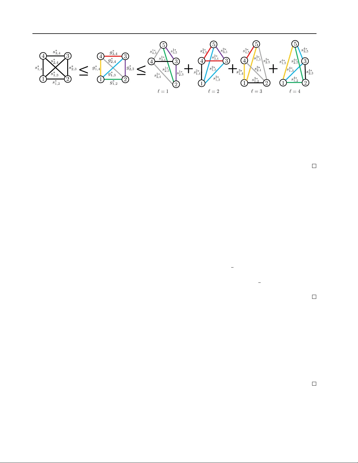
T ractable n -Metrics f or Multiple Graphs Sam Safavi 1 Jos ´ e Bento 1 Abstract Graphs are used in almost every scientiﬁc disci- pline to express relations among a set of objects. Algorithms that compare graphs, and output a closeness score, or a correspondence among their nodes, are thus extremely important. Despite the large amount of work done, many of the scal- able algorithms to compare graphs do not produce closeness scores that satisfy the intuiti ve proper - ties of metrics. This is problematic since non- metrics are known to de grade the performance of algorithms such as distance-based clustering of graphs ( Bento and Ioannidis , 2018 ). On the other hand, the use of metrics increases the performance of sev eral machine learning tasks ( Indyk , 1999 ; Clarkson , 1999 ; Angiulli and Pizzuti , 2002 ; Ack- ermann et al. , 2010 ). In this paper , we introduce a ne w f amily of multi-distances (a distance between more than two elements) that satisﬁes a general- ization of the properties of metrics to multiple elements. In the context of comparing graphs, we are the ﬁrst to show the existence of multi- distances that simultaneously incorporate the use- ful property of alignment consistency ( Nguyen et al. , 2011 ), and a generalized metric property . Furthermore, we sho w that these multi-distances can be relaxed to con vex optimization problems, without losing the generalized metric property . 1. Introduction A canonical way to check if two graphs G 1 and G 2 are similar , is to try to ﬁnd a map P from the nodes of G 2 to the nodes of G 1 such that, for many pairs of nodes in G 2 , their images in G 1 through P hav e the same connectivity relation (connected/disconnected) ( Deza and Deza , 2009 ). For equal-sized graphs, this can be formalized as d p G 1 , G 2 q ﬁ min P t~ A 1 ´ P A 2 P J ~“~ A 1 P ´ P A 2 ~u , (1) where A 1 and A 2 are the adjacency matrices of G 1 and G 2 , P and its transpose P J are permutation matrices, and, here, 1 Department of Computer Science, Boston College, Chestnut Hill, MA, USA. Correspondence to: Jos ´ e Bento < jose.bento@bc.edu > . ~ ¨ ~ is the Frobenius norm. A map P ˚ that minimizes ( 1 ) is called an optimal alignment or matc h between G 1 and G 2 . If d p G 1 , G 2 q is small (resp. large), we say G 1 and G 2 are topologically similar (resp. dissimilar). Computing d , or P ˚ , is hard ( Klau , 2009 ). Determining if d p G 1 , G 2 q “ 0 , which is the graph isomorphism problem, is not kno wn to be in P , or in NP-hard ( Babai , 2016 ). Scalable alignment algorithms, which ﬁnd an approxima- tion P to an optimal alignment P ˚ , or ﬁnd a solution to a tractable v ariant of ( 1 ) , e.g., ( Klau , 2009 ; Bayati et al. , 2013 ; Singh et al. , 2008 ; El-Kebir et al. , 2015 ), have mostly been de veloped with no concern as to whether the closeness score d obtained from the alignment P , e.g., computed via d p G 1 , G 2 q “ } A 1 P ´ P A 2 } , results in a non-metric. An exception is the recent work in ( Bento and Ioannidis , 2018 ). Indeed for the methods in, e.g., ( Klau , 2009 ; Bayati et al. , 2013 ; Singh et al. , 2008 ; El-Kebir et al. , 2015 ), the work of ( Bento and Ioannidis , 2018 ) shows that one can ﬁnd two graphs that are indi vidually similar to a third one, but not similar to each other , according to d . Furthermore, ( Bento and Ioannidis , 2018 ) shows ho w the lack of the metric prop- erties can lead to a degraded performance in a clustering task to automatically classify dif ferent graphs into the cat- egories: Barabasi Albert, Erdos-Renyi, Power Law T ree, Regular graph, and Small W orld. At the same time, the metric properties allo w us to solve se veral machine learning tasks efﬁciently ( Indyk , 1999 ; Clarkson , 1999 ; Angiulli and Pizzuti , 2002 ; Ackermann et al. , 2010 ), as we no w illustrate. Diameter estimation: Giv en a set S with | S | graphs, we can compute the maximum diameter ∆ ﬁ max G 1 ,G 2 P S d p G 1 , G 2 q by computing ` | S | 2 ˘ distances. Howe ver , if d is a metric, we know that there are at least Ω p| S |q pairs of graphs with d ě ∆ { 2 . Indeed, if d p G ˚ , G ˚ q “ ∆ , then, by the triangle inequality , for any G P S , we cannot have both d p G ˚ , G q ă ∆ { 2 and d p G ˚ , G q ă ∆ { 2 . Therefore, if we e valuate d on ran- dom pairs of graphs, we are guaranteed to ﬁnd an 1 { 2 - approximation of ∆ with only O p| S |q distance computa- tions, on av erage. Being able to compare two graphs is important in many ﬁelds such as biology ( Kalaev et al. , 2008 ; Zaslavskiy et al. , 2009a ; Kelle y et al. , 2004 ; W eskamp et al. , 2007 ), object recognition ( Conte et al. , 2004 ), dealing with ontologies T ractable n -Metrics f or Multiple Graphs ( Hu et al. , 2008 ; W ang et al. , 2016 ), computer vision ( Conte et al. , 2004 ), and social networks ( Zhang and S. Y u , 2015 ), and graph clustering ( Ma et al. , 2016 ), to name a few . In many applications, ho wever , one needs to jointly compare multiple graphs. This is t he case, for example, in aligning protein-protein interaction networks ( Singh et al. , 2008 ), recommendation systems, in the collecti ve analysis of net- works, or in the alignment of graphs obtained from brain MRI ( Papo et al. , 2014 ). The problem of jointly comparing n graphs, n ě 3 , is harder , and has been studied far less than when n “ 2 . Examples and applications include ( Pachauri et al. , 2013 ; Douglas et al. , 2018 ; Y an et al. , 2015a ; Gold and Rangarajan , 1996 ; Hu et al. , 2016 ; Park and Y oon , 2016 ; Huang and Guibas , 2013 ; Sol ´ e-Ribalta and Serratosa , 2011 ; W illiams et al. , 1997 ; Hashemifar et al. , 2016 ; Heimann et al. , 2018 ; Nassar and Gleich , 2017 ; Feizi et al. , 2016 ; Chen et al. , 2014 ). Consider the search for a function d p G 1 , ..., G n q that scores how close G 1 , ..., G n are. Ne w questions arise when n ě 3 : 1. If d produces alignments between each pair of graphs in t G 1 , . . . , G n u , should these alignments be related? What properties should they satisfy? 2. Should d satisfy similar properties to that of a metric? What properties? 3. Is it possible to ﬁnd a d that is tractable? Is it possible to impose on d the properties from 1 and 2 abov e without losing tractability? Multi-graph alignment scores, are important in man y ap- plications. F or example, man y problems require clustering using n th order interaction ( Leordeanu and Sminchisescu , 2012 ), i.e., clustering based on the similarity of groups of n elements, not just groups of two elements, as in spectral, or hierarchical clustering. Furthermore, having a score func- tion d p G 1 , . . . , G n q with some form of generalized metric property can have adv antages, similar to what ( Bento and Ioannidis , 2018 ) showed for metrics (cf. Section 4 ). In this paper , we are the ﬁrst to provide a family of similarity scores for jointly comparing multiple graphs that simultane- ously (a) giv e intuitiv e joint alignments between graphs, (b) satisfy similar properties to those of metrics, and (c) can be computed using con vex optimization methods. 2. Related work Consider three graphs G 1 , G 2 , and G 3 , and three permu- tation matrices P 1 , 2 , P 2 , 3 and P 1 , 3 , where the map P i,j is an alignment between the nodes of graphs G i and G j . An intuitiv e property that is often required for these alignments is that if P 1 , 2 maps (the nodes of) G 1 to G 2 , and if P 2 , 3 maps G 2 to G 3 , then P 1 , 3 should map G 1 to G 3 . Mathe- matically , P 1 , 3 “ P 1 , 2 P 2 , 3 . This property is often called alignment consistency . Papers that enforce this constraint, or v ariants of it, include ( Huang and Guibas , 2013 ; Pachauri et al. , 2013 ; Chen et al. , 2014 ; Y an et al. , 2015b ; a ; Zhou et al. , 2015 ; Hu et al. , 2016 ). Most of these papers focus on computer vision, i.e., the task of producing alignments between shapes, or reference points among dif ferent ﬁgures, although most of the ideas can be easily adapted to align- ing graphs. The proposed alignment algorithms are not all equally easy to solve, some in volve con vex problems, oth- ers in volv e non-con ve x or integer-v alued problems. None of these works care about the alignment scores satisfying metric-like properties. There are se veral papers that propose procedures for generat- ing multi-distances from pairwise distances, and prov e that these multi-distances satisfy intuitiv e generalizations of the metric properties to n ě 3 elements. These allo w us to use the existing works on two-graph comparisons to produce distances between multiple graphs. The simplest method is to deﬁne d p G 1 , . . . , G n q “ ř i,j Pr n s d p G i , G j q . The prob- lem with this approach is that if d p G i , G j q also produces an alignment P i,j , e.g., in ( 1 ) , these alignments are unrelated, and hence do not satisfy consistency constrains that are usu- ally desirable. An approach studied by ( Kiss et al. , 2018 ) is to deﬁne d p G 1 , . . . , G n q “ min G ř i Pr n s d p G i , G q . If each d p G i , G q also produces an alignment P i , and if we deﬁne P i,j “ P i P J j , then t P i,j u is a set of alignments that satisfy the aforementioned consistency constraint. The problem with this approach is that it tends to lead to computationally harder problems, e ven after se veral relaxations are applied (cf. Fermat distance in Section 4 ). A few other w orks that study metrics and their generalizations are ( Kiss et al. , 2018 ; Mart ´ ın et al. , 2011 ; Akleman and Chen , 1999 ). The work of ( Bento and Ioannidis , 2018 ) deﬁnes a family of metrics for comparing two graphs. Several metrics in this family are tractable, or can be reduced to solving a con vex optimization problem. Howev er, ( Bento and Ioanni- dis , 2018 ) does not consider comparing n ě 3 graphs. W e refer the reader to ( Khamsi , 2015 ) that surveys generalized metric spaces, and ( Deza and Deza , 2009 ) that provides an extensi ve re view of many distance functions along with their applications in dif ferent ﬁelds, and, in particular , discusses the generalizations of the concept of metrics in different ar - eas such as topology , probability , and algebra. The authors in ( Deza and Deza , 2009 ) also discuss sev eral distances for comparing two graphs, most of which are not tractable. 3. Notation and preliminaries W e focus on comparing graphs of equal size. A canonical way to deal with graphs with dif ferent sizes is to add dummy nodes to make them equal-sized. Many applied papers, e.g., ( Zasla vskiy et al. , 2009a ; b ; Narayanan et al. , 2011 ; Zaslavskiy et al. , 2010 ; Zhou and De la T orre , 2012 ; Gold T ractable n -Metrics f or Multiple Graphs G i i th graph P i,j Alig. of G i and G j A i Adj. mat. of G i P Set of alig. mats. n # of graphs d Dist. among n graphs m # of nodes Ω Set of adj. mats. s Alig. score S Set of sets of alig. mats. P Mat. of t P i,j u }| ¨ }| Mat. norm } ¨ } V ec. norm tr T race T able 1. Summary of main notation used. et al. , 1996 ; Y an et al. , 2015c ; Sol ´ e-Ribalta and Serratosa , 2010 ; Y an et al. , 2015a ), follow this approach. Comparing equal-sized graphs, without adding dummy nodes is still important. One application in computer vi- sion is to establish a correspondence among the nodes of n graphs, each representing a geometrical relation among m special points in n images of the same object. The user (or detection algorithm), by design, ﬁnds the same number , m , of special points in each image. See, e.g., the numer- ical experiments in ( Hu et al. , 2016 ; Shen et al. , 2015 ). Other papers that only consider equal-sized graphs include: ( L yzinski et al. , 2016 ; Pachauri et al. , 2013 ). W e also point the reader to the remark on comparing graphs of unequal size at end of Section 7 . Let r m s “ t 1 , . . . , m u . A graph, G “ p V ” r m s , E q , with node set V and edge set E , is represented by a matrix, A , whose entries are index ed by the nodes in V . W e denote the set that contains all such matrices by Ω Ď R m ˆ m . E.g., Ω can be the set of adjacency matrices, or of the matrices containing hop-distances between all pairs of nodes. Consider a set of n graphs, G “ t G 1 , G 2 , . . . , G n u . Given two graphs, G i “ p V i , E i q and G j “ p V j , E j q , from the set G , we denote a pairwise matching matrix between G i and G j by P i,j . The ro ws and columns of P i,j are indexed by the nodes in V i and V j , respectiv ely . Note that we can extract a relation between E i and E j , from a relation between V i and V j . W e denote the set of all pairwise matching matrices by P “ tt P i,j u i,j Pr n s : P i,j P R m ˆ m u . F or example, P might be all permutation matrices on m elements. Let 1: n denote the sequence 1 , . . . , n . F or A 1 , . . . , A n P Ω , we denote the ordered sequence p A 1 , . . . , A n q by A 1: n . The notation A i 1: n,n ` 1 corresponds to the sequence A 1: n , in which the i th element, A i , is r emoved and replaced by A n ` 1 . If σ is a permutation, i.e., a bijection from 1: n to 1: n such that σ p i q “ j , then A σ p 1: n q represents a sequence, whose i th element is A j . In this paper , we use } ¨ } and ~ ¨ ~ to denote vector norms and matrix norms, respectiv ely . W e now pro vide the following deﬁnitions that will be used in the next sections of the paper . In what follo ws, equality of graphs means that they are isomorphic. Deﬁnition 1. A map d : Ω 2 ÞÑ R , is a metric, if and only if, for all A, B , C P Ω : (i) d p A, B q ě 0 ; (ii) d p A, B q “ 0 , iff A “ B ; (iii) d p A, B q “ d p B , A q ; and (iv) d p A, C q ď d p A, B q ` d p B , C q . Deﬁnition 2. A map d : Ω 2 ÞÑ R is a pseudometric, if and only if it satisﬁes properties (i), (iii) and (iv) in Deﬁnition 1 , and if d p A, A q “ 0 @ A P Ω . Giv en a pseudometric d on two graphs, we deﬁne the equiv alence relation „ d in Ω as A „ d B if and only if d p A, B q “ 0 . Using the fact that d is a pseudometric, it is immediate to verify that the binary relation „ d satis- ﬁes reﬂe xivity , symmetry and transitivity . W e denote by Ω 1 “ Ω z „ d the quotient space Ω modulo „ d , and, for any A P Ω , we let r A s Ď Ω denote the equiv alence class of A . Given A 1: n , we let r A s 1: n denote pr A 1 s , . . . , r A n sq , an ordered set of sets. Deﬁnition 3. A map s : Ω 2 ˆ P ÞÑ R is called a P -scor e, if and only if, P is closed under inver sion, and for any P , P 1 P P , and A, B , C P Ω , s satisﬁes the properties: s p A, B , P q ě 0 , (2) s p A, A, I q “ 0 , (3) s p A, B , P q “ s p B , A, P ´ 1 q , (4) s p A, B , P q ` s p B , C , P 1 q ě s p A, C, P P 1 q . (5) For example, if P is the set of permutation matrices, and ~ ¨ ~ is an element-wise matrix p -norm, then s p A, B , P q “ ~ AP ´ B P ~ is a P -score. Deﬁnition 4 ( ( Bento and Ioannidis , 2018 )) . The SB- distance function induced by the norm ~ ¨ ~ : R m ˆ m ÞÑ R , the matrix D P R m ˆ m , and the set P Ď R m ˆ m is the map d S B : Ω 2 ÞÑ R , such that d S B p A, B q “ min P P P ~ AP ´ P B ~ ` tr p P J D q . The authors in ( Bento and Ioannidis , 2018 ), prove se veral conditions on Ω , P , the norm ~ ¨ ~ , and the matrix D , such that d S B is a metric, or a pseudometric. For example, if ~ ¨ ~ is an arbitrary entry-wise or operator norm, P is the set of n ˆ n doubly stochastic matrices, Ω is the set of symmetric matrices, and D is a distance matrix , then d S B is a pseudometric. 4. n -metrics f or multi-graph alignment One can generalize the notion of a (pseudo) metric to n ě 3 elements. T o this aim, we consider the follo wing deﬁnitions. Deﬁnition 5. A map d : Ω n ÞÑ R , is an n -metric, if and only if, for all A 1 , . . . , A n P Ω , d p A 1: n q ě 0 , (6) d p A 1: n q “ 0 , iff A 1 “ . . . “ A n , (7) d p A 1: n q “ d p A σ p 1: n q q , (8) d p A 1: n q ď ř n i “ 1 d p A i 1: n,n ` 1 q . (9) T ractable n -Metrics f or Multiple Graphs According to Deﬁnition 5 , a 2 -metric is a metric as per Def- inition 1 . In the sequel, we refer to properties ( 6 ) , ( 7 ) , ( 8 ) , and ( 9 ) , as non-negati vity , identity of indiscernibles, sym- metry , and generalized triangle equality (GTI), respectiv ely . Deﬁnition 6. A map d : Ω n ÞÑ R , is a pseudo n -metric, if and only if it satisﬁes pr operties ( 6 ) , ( 8 ) and ( 9 ) , and for any A P Ω , d satisﬁes the property of self-identity d p A, ¨ ¨ ¨ , A q “ 0 . (10) Revisiting diameter estimation: n -metrics have sev eral advanta ges over non- n -metrics. F or n “ 2 , this is sho wn by ( Bento and Ioannidis , 2018 ) and references therein: metrics allow se veral ML algorithms to ﬁnish faster , and improv e the accuracy in tasks such as clustering graphs. Some of these advantages also extend to n ą 2 . For example, it is straightforward to see that, if we generalize the diameter estimation problem in Sec. 1 to n “ 3 , we can compute a 1 { 3 -approximation of max G 1 ,G 2 ,G 3 P S d p G 1 , G 2 , G 3 q in ex- pected time O p n 2 q , compared to O p n 3 q for a non- n -metric. Considering the runtime of distance-based clustering using n th or der interaction ( Purkait et al. , 2017 ), and just like for n “ 2 , n -metrics, n ą 2 , also impro ve runtime, because the GTI lets us av oid dealing with all n -distances. W e no w deﬁne two functions that satisfy the properties of (pseudo) n -metrics. 4.1. A ﬁrst attempt: F ermat distances Deﬁnition 7. Given a map d : Ω 2 ÞÑ R , the F ermat dis- tance function induced by d , is the map d F : Ω n ÞÑ R , deﬁned by d F p A 1: n q “ min B P Ω n ÿ i “ 1 d p A i , B q . (11) In the context of multiple graph alignment, d is an align- ment score between two graphs, and d F aims to ﬁnd a graph, represented by B , that aligns well with all the graphs, rep- resented by A 1: n . Thus, d F p A 1: n q can be interpreted as an alignment score computed as the sum of alignment scores between each A i and B . If we think of A 1: n as a cluster of graphs, we can think of B as its center . Theorem 1. If d is a pseudometric, then the F ermat distance function induced by d is a pseudo n -metric. The proof of Theorem 1 is a direct adaptation of the one in ( Kiss et al. , 2018 ), and is included in Appendix B for completeness. For example, the Fermat distance function induced by an SB-distance function with a distance matrix D “ 0 is d F p A 1: n q “ min B P Ω , t P i uP P n n ÿ i “ 1 ~ A i P i ´ P i B ~ . Despite its simplicity , the abov e optimization problem is not easy to solve in general, even when it is a continuous smooth optimization problem. For example, if P is the set of doubly stochastic matrices, B is the set of real matrices with entries in r 0 , 1 s , and ~ ¨ ~ is the Frobenius norm, the problem is non-con ve x due to the product P B that appears in the objectiv e function. The potential complexity of computing d F motiv ates the following alternati ve deﬁnition. 4.2. A better approach: G -align distances Deﬁnition 8. Given a map s : Ω 2 ˆ P ÞÑ R , the G -align distance function induced by s , is the map d G : Ω n ÞÑ R , deﬁned by d G p A 1: n q “ min P P S 1 2 ÿ i,j Pr n s s p A i , A j , P i,j q , (12) wher e S “ tt P i,j u i,j Pr n s : P i,j P P , @ i, j P r n s , P i,k P k,j “ P i,j , @ i, j, k P r n s , P i,i “ I , @ i P r n su . (13) Remark 1. F r om the deﬁnition of S , it is implied that I P P and that, if P P S , then P i,j P j,i “ P i,i “ I ô p P i,j q “ p P j,i q ´ 1 @ i, j P r n s , hence t P i,j u ar e invertible . Remark 2. In ( 13 ) , we r efer to the pr operty P i,j P j,k “ P i,k , @ i, j, k P r n s , as the alignment consistency of P P S . The follo wing Lemma, provides an alternati ve deﬁnition for the G -align distance function. Lemma 1. If s is a P -scor e, then d G p A 1: n q “ min P P S ÿ i,j Pr n s , i ă j s p A i , A j , P i,j q . (14) Pr oof. ÿ i,j Pr n s s p A i , A j , P i,j q “ ÿ i Pr n s s p A i , A i , P i,i q` ÿ i,j Pr n s : i ă j p s p A i , A j , P i,j q ` s p A j , A i , P j,i qq . (15) If P P S , then P i,i “ I and P j,i “ p P i,j q ´ 1 . Thus, since s is a P -score, s p A i , A i , P i,i q “ s p A i , A i , I q “ 0 , by prop- erty ( 3 ) , and s p A j , A i , P j,i q “ s p A i , A j , P i,j q , by property ( 4 ). Therefore, ÿ i,j Pr n s s p A i , A j , P i,j q “ 2 ÿ i,j Pr n s , i ă j s p A i , A j , P i,j q , and the proof follows. Note that, if s p A, B , P q “ ~ AP ´ P B ~ , for some element- wise matrix norm, n “ 2 , and P is the set of permutations on m elements, then according to Lemma 1 , d G p A, B q “ d S B p A, B q , for D “ 0 . In general, we can deﬁne a gener- alized SB-distance function induced by a matrix D , a set P Ď R m ˆ m and a map s : Ω 2 ˆ P ÞÑ R as d S B p A, B q “ min P P P s p A, B , P q ` tr p P J D q , (16) T ractable n -Metrics f or Multiple Graphs and in vestigate the conditions on s , P and D , under which ( 16 ) represents a (pseudo) metric. The following lemma leads to an equiv alent deﬁnition for the G -align distance function, which, among other things, reduces the optimization problem in ( 12 ) , to ﬁnding n dif fer- ent matrices rather that n 2 ´ n matrices that need to satisfy the alignment consistency . Lemma 2. If S 1 “ tt P i,j u i,j Pr n s : P i,j P P and P i,j “ Q i p Q j q ´ 1 , @ i, j P r n s , for some matrices t Q i u Ď P u , then S 1 “ S . Pr oof. W e ﬁrst prove that S Ď S 1 . Let P P S . Deﬁne Q i “ P i,n P P for all i P r n s . If i, j P r n ´ 1 s , then, by deﬁnition, P i,j “ P i,n P n,j “ P i,n p P j,n q ´ 1 “ Q i p Q j q ´ 1 . This prov es that P P S 1 . W e now prove that S 1 Ď S . Let P P S 1 . For any i, j, k P r n s , we hav e P i,k P k,j “ Q i p Q k q ´ 1 Q k p Q j q ´ 1 “ Q i p Q j q ´ 1 “ P i,j . It also follo ws that P i,j “ Q i p Q j q ´ 1 “ p Q j p Q i q ´ 1 q ´ 1 “ p P j,i q ´ 1 , and P i,i “ Q i p Q i q ´ 1 “ I . Therefore, P P S . W e complete this section with the follo wing theorem, whose detailed proof is provided in Appendix C . Theorem 2. If s is a P -scor e, then the G -align function induced by s is a pseudo n -metric. In Appendix A , we discuss the special case of P being the set of orthogonal matrices. In this case, we can simplify both eq. ( 11 ), and eq. ( 12 ), and compute them efﬁciently . 5. n -metrics on quotient spaces The theorems in Section 4 are stated for pseudometrics. Howe ver , it is easy to obtain an n -metric from a pseudo n -metric for both d F and d G using quotient spaces. In these spaces, ( 7 ) holds almost tri vially (with A i replaced by its equiv alent class r A i s ), and the important question is whether the equi valent classes of graphs are meaningful and useful. The proofs for the theorems in this section are Appendices G and H . Theorem 3. Let d be a pseudometric for two gr aphs, d F be the F ermat distance function for n graphs induced by d , and Ω 1 “ Ω z „ d . Let d 1 F : Ω 1 n ÞÑ R be such that d 1 F pr A s 1: n q “ d F p A 1: n q . (17) Then, d 1 F is an n -metric. Theorem 4. Let s be a P -scor e. Let d G 2 : Ω 2 ÞÑ R be the G -align distance function for two graphs induced by s , and d G : Ω n ÞÑ R be the G -align distance function for n graphs induced by s . Let Ω 1 “ Ω z „ d G 2 , and d 1 G : Ω 1 n ÞÑ R be such that d 1 G pr A s 1: n q “ d G p A 1: n q . (18) Then, d 1 G is an n -metric. 6. The generalized triangle inequality f or d G : an illustrative example While it is straightforward to show that d G satisﬁes the properties of non-negati vity , symmetry and self-identity, the proof for the generalized triangle inequality is more in- volv ed. T o give the reader a ﬂav or of the proof, we now prov e that the G -align function satisﬁes the generalized tri- angle inequality when n “ 4 . W e consider a set of n “ 4 graphs, G “ t G 1 , G 2 , G 3 , G 4 u , and a reference graph G 5 , represented by matrices, A 1 , A 2 , A 3 , A 4 P Ω and A 5 P Ω , respecti vely . W e will show that d G p A 1:4 q ď 4 ÿ ` “ 1 d G p A ` 1:4 , 5 q . (19) Let P ˚ “ t P ˚ i,j u P S be an optimal value for P in the optimization problem corresponding to the left-hand-side (l.h.s) of ( 19 ) . W e deﬁne s ˚ i,j “ s p A i , A j , P ˚ i,j q for all i, j P r 4 s . W e also deﬁne s ` ˚ i,j “ s p A i , A j , P ` ˚ i,j q for all i, j P r 5 s , ` P r 4 szt i, j u , in which P ` ˚ “ t P ` ˚ i,j u P S is an optimal value for P in the optimization problem associated to d G p A ` 1:4 , 5 q on the r .h.s of ( 19 ) . Note that, according to ( 4 ) , and the fact that P ˚ i,j “ p P ˚ j,i q ´ 1 (since P ˚ P S ), we hav e s ˚ i,j “ s ˚ j,i , and s ` ˚ i,j “ s ` ˚ j,i . (20) Moreov er , according to ( 5 ), we hav e s p A i , A j , P ` ˚ i,k P ` 1 ˚ k,j q ď s ` ˚ i,k ` s ` 1 ˚ k,j , (21) and, in the particular case when ` “ ` 1 , we hav e s ` ˚ i,j ď s ` ˚ i,k ` s ` ˚ k,j . (22) From the deﬁnition of d G in Lemma 1 , we hav e ÿ i,j Pr 4 s , i ă j s ˚ i,j ď ÿ i,j Pr 4 s , i ă j s p A i , A j , Γ i,j q , (23) where Γ i,j “ Γ i Γ ´ 1 j , and t Γ i u are any set of in vertible ma- trices in P . Note that from Lemma 2 , t Γ i,j u P S . Consider the following choices for Γ i ’ s : Γ 1 “ P 4 ˚ 1 , 5 ; Γ 2 “ P 1 ˚ 2 , 5 ; Γ 3 “ P 2 ˚ 3 , 5 ; Γ 4 “ P 3 ˚ 4 , 5 . (24) W e deﬁne g ˚ i,j “ s p A i , A j , Γ i Γ ´ 1 j q , in which Γ i ’ s are cho- sen according to ( 24 ). W e can then rewrite ( 23 ) as ÿ i,j Pr 4 s , i ă j s ˚ i,j ď ÿ i,j Pr 4 s , i ă j g ˚ i,j . (25) W e use Fig. 1 to bookkeep all the terms in volv ed in proving ( 19 ) . In particular, the ﬁrst inequality in Fig. 1 provides a pictorial representation of ( 25 ) . In this ﬁgure, each circle represents a graph in G , and a line between G i and G j represents the P -score between A i and A j . In the diagram T ractable n -Metrics f or Multiple Graphs ≤ + + + ≤ Figure 1. Generalized triangle equality of d G for n “ 4 graphs. on the left, each P -score corresponds to the optimal pairwise matching between G i and G j associated to d G p A 1:4 q in ( 19 ) , whereas in the diagram in the middle, each P -score corresponds to the suboptimal matching between G i and G j , where the pairwise matching matrices are chosen according to ( 24 ). Using ( 21 ), follo wed by ( 20 ) we get ÿ i,j Pr 4 s , i ă j g ˚ i,j ď p s 4 ˚ 1 , 5 ` s 1 ˚ 2 , 5 q ` p s 4 ˚ 1 , 5 ` s 2 ˚ 3 , 5 q ` p s 4 ˚ 1 , 5 ` s 3 ˚ 4 , 5 q ` p s 1 ˚ 2 , 5 ` s 2 ˚ 3 , 5 q ` p s 1 ˚ 2 , 5 ` s 3 ˚ 4 , 5 q ` p s 2 ˚ 3 , 5 ` s 3 ˚ 4 , 5 q . The abov e inequality is also depicted in Fig. 1 , where each diagram on the r .h.s of the second inequality represents d G p A ` 1:5 q in ( 19 ) for a different ` P r 4 s . Applying ( 22 ) to the r .h.s. of the abo ve inequality , one can see that each one of the terms in parenthesis, distinguished with a dif ferent color , is upper bounded by the sum of the terms with the same color in the diagram in the r .h.s of the second inequality in Fig. 1 . This completes the proof. 7. Moving towards tractability The follo wing lemmas are the building blocks to wards a relaxation of d G that is also easy to compute for choices of P other than orthonormal matrices. In this section, ~ ¨ ~ ˚ denotes the nuclear norm. Lemma 3. Given t P i,j u i,j Pr n s such that P i,j P R m ˆ m for all i, j P r n s , let P P R nm ˆ nm have n 2 blocks, such that the p i, j q th block is P i,j . Let S 2 “ tt P i,j u i,j Pr n s : rank p P q “ m, P i,j P P , @ i, j P r n s , P i,i “ I , @ i P r n su . (26) W e have that S 2 “ S , wher e S is as deﬁned in ( 13 ) . Pr oof. Let P P R nm ˆ nm , with blocks t P i,j u i,j Pr n s P S 2 . Since rank p P q “ m , from the singular v alue decomposition of P , we can write P “ AB J where A, B P R mn ˆ m . Let A “ r A 1 ; . . . ; A n s , where A i P R m ˆ m and, similarly , let B “ r B 1 ; . . . ; B n s , where B i P R m ˆ m . It follows that P i,j “ A i B J j . Since P i,i “ I , we have A i B J i “ I , which implies that P i,j “ A i A ´ 1 j . By Lemma 2 , this in turn implies that t P i,j u i,j Pr n s satisfy the alignment consistency property . Therefore, t P i,j u i,j Pr n s P S , and thus S 2 Ď S . Let P “ t P i,j u i,j Pr n s P S . By Lemma 2 , P i,j “ Q i Q ´ 1 j for some in vertible matrices t Q i u i Pr n s . Let A, B P R mn ˆ m , with A “ r Q 1 ; . . . ; Q n s and B “ rp Q ´ 1 1 q J , . . . , p Q ´ 1 n q J s . Let P denote the mn ˆ mn block matrix with P i,j as the p i, j q th block. W e have P “ AB J . Thus m ě rank p P q ě rank p A q ě rank p Q 1 q “ m , which implies that t P i,j u i,j Pr n s P S 2 , and therefore S Ď S 2 . Lemma 4. [ ( Huang and Guibas , 2013 ), Proposition 1] Let P be the set of m ˆ m permutation matrices. Given t P i,j u i,j Pr n s such that P i,j P P for all i, j P r n s , let P P R nm ˆ nm have n 2 blocks, such that the p i, j q th block is P i,j . Let S 3 “ tt P i,j u i,j Pr n s : P i,j P P , @ i, j P r n s , P ľ 0 , P i,i “ I , @ i P r n su . (27) W e have that S 3 “ S , wher e S is as deﬁned in ( 13 ) . Lemma 5. F or any P P R nm ˆ nm with P ii “ 1 for all i P r nm s , we have ~ P ~ ˚ ě nm . Pr oof. Let P 1 “ 1 2 p P ` P J q . W e hav e nm “ tr p P q “ tr p P 1 q “ ř i Pr nm s λ i p P 1 q ď ř i Pr nm s | λ i p P 1 q| “ ř i Pr nm s σ i p P 1 q “ ~ P 1 ~ ˚ ď 1 2 p~ P ~ ˚ ` ~ P J ~ ˚ q “ ~ P ~ ˚ , where λ i p¨q and σ i p¨q denote the i th eigen value and the i th singular value of p¨q , respecti vely . Lemma 6. Let P be a subset of the orthogonal matrices. Let t P i,j u i,j Pr n s P S , and P be the mn ˆ nm block matrix with P i,j as the p i, j q th block. W e have ~ P ~ ˚ “ mn . Pr oof. Since t P i,j u i,j Pr n s P S are alignment-consistent, we can write P i,j “ P i,n P ´ 1 j,n for all i, j P r n s . Since P j,n P P , it must be orthogonal. Hence, P i,j “ P i,n P J j,n , and we can write P “ AA J , where A “ r Q 1 ; . . . ; Q n s P R nm ˆ m , and Q i “ P i,n . Since P is positive semi-deﬁnite, its eigenv alues are equal to its singular values, which are non-negati ve, and thus ~ P ~ ˚ “ tr p AA J q “ tr p A J A q “ ř i Pr n s tr p Q J i Q i q “ ř i Pr n s tr p I q “ mn . Inspired by Lemmas 3 , 5 , and 6 , to obtain a continuous relaxation of d G , we relax the rank constraint rank p P q ď m to ~ P ~ ˚ ď mn , use a function s that is a continuous func- tion of P , and use a set P that is compact and contains T ractable n -Metrics f or Multiple Graphs a non-empty ball around I . Alternatively , we can impose that P j,i “ P J i,j , which was the case when P only con- tained orthonormal matrices, and relax the rank constraint to tr p P q ď mn and P ľ 0 , i.e., P is a symmetric matrix with non-negati ve eigen values. Note that since we want P i,i “ I for all i P r n s , we can drop the trace constraint. The relaxation to P ľ 0 can also be justiﬁed by Lemma 4 and relaxing the constraint that P must be the set of permu- tations. Deﬁnition 9. Let P Ď R m ˆ m be compact and contain a non-empty ball ar ound I . Let P i,j P P for all i, j P r n s , and P be the mn ˆ nm block matrix with P i,j as the p i, j q th block. Given a map s : Ω 2 ˆ P ÞÑ R , such that s p¨ , ¨ , P q is continuous for all P P P , the continuous G -align distance function induced by s , is the map d c G : Ω n ÞÑ R , deﬁned by d c G p A 1: n q “ min P i,j P P @ i,j Pr n s , P i,i “ I @ i Pr n s , ~ P ~ ˚ ď mn 1 2 ÿ i,j Pr n s s p A i , A j , P i,j q , (28) and the symmetric continuous G -align distance function induced by s , is the map d sc G : Ω n ÞÑ R , deﬁned by d sc G p A 1: n q “ min P i,j P P @ i,j Pr n s , P i,i “ I @ i Pr n s , P ľ 0 1 2 ÿ i,j Pr n s s p A i , A j , P i,j q . (29) Remark 3. Both optimization problems ar e continuous optimization pr oblems, although the y ar e potentially non- con vex. However , for several natur al choices of s , e.g ., s p A, B , P q “ ~ AP ´ P B ~ , and con vex P , both ( 28 ) and ( 29 ) can be computed via con vex optimization. W e ﬁnish this section, by sho wing that the abo ve continuous distance functions, d c G and d sc G , are pseudo n -metrics. In what follows, we let } ¨ } and ~ ¨ ~ 2 denote the Euclidean norm and matrix operator norm, respectiv ely . W e will use the following deﬁnition. Deﬁnition 10. A map s : Ω 2 ˆ P ÞÑ R is called a modiﬁed P -scor e, if and only if, P is closed under transposition and multiplication, for any P P P , ~ P ~ 2 ď 1 , and for any P , P 1 P P , and A, B , C P Ω , s satisﬁes the properties: s p A, B , P q ě 0 , (30) s p A, A, I q “ 0 , (31) s p A, B , P q “ s p B , A, P J q , (32) s p A, B , P q ` s p B , C , P 1 q ě s p A, C, P P 1 q . (33) For example, if P is the set of doubly stochastic matrices, Ω is a subset of the symmetric matrices, and ~ ¨ ~ is an element- wise matrix p -norm, then s p A, B , P q “ ~ AP ´ B P ~ is a modiﬁed P -score. W e no w provide the main result of this section. Theorem 5. If s is a modiﬁed P -scor e, then the symmet- ric continuous G -align distance function induced by s is a pseudo n -metric. Remark 4. A theor em with slightly differ ent assumptions can be stated and pr oved about the d c G . Under appro- priately deﬁned equivalent classes, we can also obtain n - metrics fr om ( 28 ) and ( 29 ) (cf. Section 5 ). Graphs of different sizes: W e note that in this section, un- like in Sec. 4 , P ij does not need to be inv ertible. Therefore, it is possible to extend the (symmetric) continuous G -align distance function to consider graphs of unequal sizes. W e could, e.g., allow P ij to be rectangular of size m i by m j (resp. the node sizes of graph G i and G j ), which w ould still result in P being square. If P ij ’ s were previously doubly stochastic matrices, no w , the ro w sums (or column sums, but not both) would be allowed to be ď 1 . This would model unmatched nodes, and av oid non-trivial solutions for Eqs. ( 28 ) and ( 29 ), i.e., P i,j “ 0 when i ‰ j . 8. Numerical experiments W e do two experiments comparing our tool against two state-of-the-art non- n -metrics (from computer vision) and one simpler approach. Code for these comparison can be found in http://github.com/bentoayr/ n- metrics . This repository includes code to compute some of our n -metrics, as well as code for the other methods, which is publicly av ailable and that can be found through links in their respecti ve papers, and which was copied into our repository for con venience. The two competing algorithms are matchSync ( Pachauri et al. , 2013 ), and mOpt ( Y an et al. , 2015a ). The simpler ap- proach, P airwise , deﬁnes d p G 1 , ..., G n q “ ř i ą j d p G i , G j q , where each d p G i , G j q , is computed using ( Cho et al. , 2010 ). All of these algorithms output a set of permutation matrices t P i,j u , where P i,j tells ho w the nodes of graph i and j are matched. Both matchSync , and mOpt try to enforce the alignment consistency property on t P i,j u , while P airwise computes each P i,j independently . F or our algorithm, we use ( 28 ) , with P being the set of doubly stochastic matrices, and s p A, B , P q “ ~ AP ´ P B ~ Fro . F or comparison sake, after we compute t P i,j u using our algorithm, we sometimes project each P i,j onto the set of permutation matrices, which amounts to solving a maximum weight matching pr oblem . 8.1. Multiple graph alignment experiment W e generate one Erd ¨ os-–R ´ enyi graph with edge probability 0 . 5 , and 7 other graphs which are a small perturbation of the original graph (we ﬂip edges with 0 . 05 probability), such that we know the joint optimal alignment of these n “ 8 graphs, i.e. P ˚ i,j “ I . W e then randomly permute the labels of these graphs such that the new joint optimal alignment T ractable n -Metrics f or Multiple Graphs is kno wn but non-trivial, i.e. P ˚ i,j ‰ I . W e then use our n -metric, and the other non- n -metrics, to ﬁnd an alignment between the graphs. Finally , we compare the alignments produced by the different methods to the optimal alignment. W e repeat this 30 times, on random instances. For each set of permutations t P i,j u giv en by the different algorithms we compute the alignment quality (A Q) and the alignment consistency (A C). A Q “ 1 ´ ř n ´ 1 i “ 1 ř n j “ i ` 1 ~ P i,j ´ P ˚ i,j ~{ 2 mn p n ´ 1 q{ 2 , A C “ 1 ´ ř n r “ 1 ř n ´ 1 i “ 1 ř n j “ i ` 1 ~ P i,j ´ P i,r P r,j ~{ 2 mn 2 p n ´ 1 q{ 2 , where ~ ¨ ~ is the Frobenius norm. W e obtain the following av erage accuracy (over 30 tests), and standard deviations. Note that, by design, mOpt and matchSync hav e A C = 1. Ours mOpt matchSync P airwise A Q 0 . 94 ˘ 0 . 01 0 . 91 ˘ 0 . 02 0 . 90 ˘ 0 . 02 0 . 88 ˘ 0 . 02 A C 0 . 92 ˘ 0 . 07 1 . 0 ˘ 0 . 0 1 . 0 ˘ 0 . 0 0 . 85 ˘ 0 . 02 In Appendix J , we include an histogram with the distrib ution of values for these tw o quantities. 8.2. Graph clustering via hypergraph cut experiment W e b uild two clusters of graphs, each obtained by generat- ing (i) a Erd ¨ os-–R ´ enyi graph with edge probability 0 . 7 as the cluster center , and (ii) 9 other graphs that are a small perturbation of (i). Graphs in (ii) are generated just like in Section 8.1 . W e then try to recover the true clusters using different n -distances. For each n -distance, we b uild a hypergraph with 20 nodes ( 1 node per graph) and 100 hyperedges. Each hyperedge is built by randomly connecting 3 nodes (out of 20 ), for which the distance between their graphs is belo w a certain threshold. This threshold is later tuned to minimize each algorithm’ s clustering error (deﬁne belo w). Ideally , most h y- peredges should not include graphs in dif f erent clusters. W e then use the algorithm of ( V azquez , 2009b ), whose code can be found in ( V azquez , 2009a ) and which is included in our repositories for con venience, to ﬁnd a minimum cut of the hypergraph that di vides it into two equal-sized parts. These hyper-subgraphs are our predicted clusters. The clustering err or is the fraction of misclassiﬁed graphs times two , such that the worst possible algorithm, a random guess, giv es an avg. error of 1 . W e repeat this 50 times. F or each algorithm, we use the same threshold in all 50 repetitions. This experiment does not require an alignment between graphs but only a distance d . For algorithms that out- put an alignment t P i,j u , this distance is computed as 1 2 ř i,j ~ A i P i,j ´ P i,j A j ~ Fro . For our algorithm, we cal- culate this distance by ﬁrst projecting t P i,j u onto the per- mutation matrices, which we denote as Ours , and we also calculate this distance directly as in ( 28 ) , which we denote as Ours* . W e report the a verage error in the follo wing table. The standard deviation of the mean are all 0 . 04 except for Ours* which is 0 . 05 . Ours* Ours mOpt matchSync P airwise 0 . 40 0 . 44 0 . 44 0 . 49 0 . 46 In Appendix K we include an histogram with the distribution of errors for the different algorithms. 9. Future w ork It is possible to deﬁne the notion of a (pseudo) p C, n q - metric , as a map that satisﬁes the following more strin- gent generalization of the generalized triangle inequality: d p A 1: n q ď C ˆ ř n i “ 1 d p A i 1: n,n ` 1 q . The authors in ( Kiss et al. , 2018 ) prove that the d F is a (pseudo) p C, n q -metric with 1 n ´ 1 ď C ď 1 t n 2 u . Any (pseudo) p C, n q -metric with C ď 1 is also a (pseudo) n - metric. It is an open problem to determine the lar gest con- stant C , for which d G , d c G or d sc G are a (pseudo) p C, n q - metric, and whether C ă 1 ? W e also plan to test if the claim in ( V ijayan et al. , 2017 ), which states that in se veral scenarios calculating and using pairwise alignments is better than calculating and using joint alignments, holds for the n -metrics we introduced. W e plan to de velop fast and scalable solvers to compute our n -metrics. The objecti ve function of our n -metrics in volves a large number of sums, in turn in volving variables that are coupled by the alignment consistenc y constraint, or its relaxed equiv alent. This makes the use of decomposition- coordination methods very attracti ve. In particular, we plan to test solvers based on the Alternating Direction Method of Multipliers (ADMM). Although not strictly a ﬁrst -order method, it is very fast and, with proper tuning, it achiev es a con vergence rate that is as fast as the fastest possible ﬁrst- order method ( Fran c ¸ a and Bento , 2016 ; Nesterov , 2013 ). Furthermore, it has been used as an heuristic to solve many non-con vex, ev en combinatorial, problems ( Bento et al. , 2013 ; 2015 ; Zoran et al. , 2014 ; Mathy et al. , 2015 ), and can be less af fected by the topology of the communication network in a cluster than, e.g. Gradient Descent ( Fran c ¸ a and Bento , 2017b ; a ). Finally , ADMM parallelizes well on share-memory multiprocessor systems, GPUs, and com- puter clusters ( Boyd et al. , 2011 ; Parikh and Boyd , 2014 ; Hao et al. , 2016 ). T ractable n -Metrics f or Multiple Graphs References Marcel R Ackermann, Johannes Bl ¨ omer , and Christian Sohler . Clustering for metric and nonmetric distance measures. ACM T ransactions on Algorithms (T ALG) , 6 (4):59, 2010. E. Akleman and J. Chen. Generalized distance functions. In Shape Modeling and Applications, 1999. Proceedings. Shape Modeling International’99. International Confer - ence on , pages 72–79. IEEE, 1999. Fabrizio Angiulli and Clara Pizzuti. Fast outlier detection in high dimensional spaces. In Eur opean Confer ence on Principles of Data Mining and Knowledge Discovery , pages 15–27. Springer , 2002. L ´ aszl ´ o Babai. Graph isomorphism in quasipolynomial time. In Pr oceedings of the forty-eighth annual A CM sympo- sium on Theory of Computing , pages 684–697. ACM, 2016. Chanderjit Bajaj. Proving geometric algorithm non- solvability: An application of factoring polynomials. Journal of Symbolic Computation , 2(1):99–102, 1986. M. Bayati, D. F . Gleich, A. Saberi, and Y . W ang. Message-passing algorithms for sparse network align- ment. A CM T ransactions on Knowledge Discovery fr om Data (TKDD) , 7(1):3, 2013. Jose Bento and Stratis Ioannidis. A family of tractable graph distances. In Pr oceedings of the 2018 SIAM In- ternational Confer ence on Data Mining , pages 333–341. SIAM, 2018. Jos ´ e Bento, Nate Derbinsky , Javier Alonso-Mora, and Jonathan S Y edidia. A message-passing algorithm for multi-agent trajectory planning. In Advances in neural information pr ocessing systems , pages 521–529, 2013. Jos ´ e Bento, Nate Derbinsky , Charles Mathy , and Jonathan S Y edidia. Proximal operators for multi-agent path planning. In AAAI , pages 3657–3663, 2015. S Boyd, N Parikh, E Chu, B Peleato, and J Eckstein. Dis- tributed optimization and statistical learning via the alter- nating direction method of multipliers. F oundations and T r ends® in Machine Learning , 3(1):1–122, 2011. Y uxin Chen, Leonidas J Guibas, and Qi-Xing Huang. Near- optimal joint object matching via con vex relaxation. arXiv pr eprint arXiv:1402.1473 , 2014. Minsu Cho, Jungmin Lee, and Kyoung Mu Lee. Reweighted random walks for graph matching. In Eur opean confer- ence on Computer vision , pages 492–505. Springer , 2010. Kenneth L Clarkson. Nearest neighbor queries in metric spaces. Discr ete & Computational Geometry , 22(1):63– 93, 1999. Ernest J Cockayne and Zdzislaw A Melzak. Euclidean constructibility in graph-minimization problems. Mathe- matics Magazine , 42(4):206–208, 1969. Michael B Cohen, Y in T at Lee, Gary Miller, Jakub Pachocki, and Aaron Sidford. Geometric median in nearly linear time. In Pr oceedings of the forty-eighth annual A CM symposium on Theory of Computing , pages 9–21. A CM, 2016. D. Conte, P . Foggia, C. Sansone, and M. V ento. Thirty years of graph matching in pattern recognition. International journal of pattern r ecognition and artiﬁcial intelligence , 18(03):265–298, 2004. M. M. Deza and E. Deza. Encyclopedia of distances. In Encyclopedia of Distances , pages 1–583. Springer , 2009. Joel Douglas, Ben Zimmerman, Alexei K opylov , Jiejun Xu, Daniel Sussman, and V ince L yzinski. Metrics for ev aluating network alignment. GT A3 at WSDM , 2018. Mohammed El-Kebir , Jaap Heringa, and Gunnar W Klau. Natalie 2.0: Sparse global netw ork alignment as a special case of quadratic assignment. Algorithms , 8(4):1035– 1051, 2015. S. Feizi, G. Quon, M. Recamonde-Mendoza, M. Medard, M. Kellis, and A. Jadbabaie. Spectral alignment of graphs. arXiv pr eprint arXiv:1602.04181 , 2016. G. Fran c ¸ a and J. Bento. An explicit rate bound for ov er- relaxed admm. In Information Theory (ISIT), 2016 IEEE International Symposium on , pages 2104–2108. IEEE, 2016. Guilherme Fran c ¸ a and Jos ´ e Bento. How is distributed admm affected by network topology? arXiv preprint arXiv:1710.00889 , 2017a. Guilherme Fran c ¸ a and Jos ´ e Bento. Markov chain lifting and distributed ADMM. IEEE Signal Pr ocessing Letters , 24 (3):294–298, 2017b. S. Gold and A. Rangarajan. A graduated assignment algo- rithm for graph matching. IEEE T ransactions on pattern analysis and machine intelligence , 18(4):377–388, 1996. Stev en Gold, Anand Rangarajan, et al. Softmax to sof- tassign: Neural network algorithms for combinatorial optimization. J ournal of Artiﬁcial Neural Networks , 2(4): 381–399, 1996. T ractable n -Metrics f or Multiple Graphs Ning Hao, AmirReza Oghbaee, Mohammad Rostami, Nate Derbinsky , and Jos ´ e Bento. T esting ﬁne-grained par- allelism for the admm on a factor -graph. In P arallel and Distributed Pr ocessing Symposium W orkshops, 2016 IEEE International , pages 835–844. IEEE, 2016. S. Hashemifar , Q. Huang, and J. Xu. Joint alignment of multiple protein–protein interaction networks via con ve x optimization. J ournal of Computational Biology , 23(11): 903–911, 2016. M. Heimann, H. Shen, and D. K outra. Node representa- tion learning for multiple networks: The case of graph alignment. arXiv pr eprint arXiv:1802.06257 , 2018. A. J. Hoffman, H. W . W ielandt, et al. The variation of the spectrum of a normal matrix. Duke Mathematical Journal , 20(1):37–39, 1953. N. Hu, B. Thibert, and L. Guibas. Distributable consistent multi-graph matching. arXiv pr eprint arXiv:1611.07191 , 2016. W . Hu, Y . Qu, and G. Cheng. Matching large ontologies: A divide-and-conquer approach. Data & Knowledge Engineering , 67(1):140–160, 2008. Q. Huang and L. Guibas. Consistent shape maps via semideﬁnite programming. In Computer Graphics F o- rum , volume 32, pages 177–186. W iley Online Library , 2013. P Indyk. Sublinear time algorithms for metric space prob- lems. In Pr oceedings of the thirty-ﬁrst annual A CM sym- posium on Theory of computing , pages 428–434. A CM, 1999. M. Kalae v , M. Smoot, T . Ideker , and R. Sharan. Network- blast: comparative analysis of protein networks. Bioin- formatics , 24(4):594–596, 2008. B. P . Kelle y , B. Y uan, F . Le witter , R. Sharan, B. R. Stock- well, and T . Ideker . Pathblast: a tool for alignment of protein interaction networks. Nucleic acids r esear ch , 32 (suppl 2):W83–W88, 2004. M. A. Khamsi. Generalized metric spaces: a surve y . Journal of F ixed P oint Theory and Applications , 17(3):455–475, 2015. Gergely Kiss, Jean-Luc Marichal, and Bruno T eheux. A generalization of the concept of distance based on the simplex inequality . Beitr ¨ age zur Algebr a und Geome- trie/Contributions to Alg ebra and Geometry , 59(2):247– 266, 2018. Gunnar W Klau. A new graph-based method for pairwise global network alignment. BMC bioinformatics , 10(1): S59, 2009. Marius Leordeanu and Cristian Sminchisescu. Efﬁcient h y- pergraph clustering. In Artiﬁcial Intelligence and Statis- tics , pages 676–684, 2012. V ince L yzinski, Donniell Fishkind, Marcelo Fiori, Joshua V ogelstein, Carey Priebe, and Guillermo Sapiro. Graph matching: Relax at your o wn risk. IEEE T ransactions on P attern Analysis & Mac hine Intelligence , (1):1–1, 2016. Guixiang Ma, Lifang He, Bokai Cao, Jiawei Zhang, S Y u Philip, and Ann B Ragin. Multi-graph clustering based on interior-node topology with applications to brain net- works. In J oint Eur opean Conference on Mac hine Learn- ing and Knowledge Discovery in Databases , pages 476– 492. Springer , 2016. J. Mart ´ ın, G. Mayor , and O. V alero. Functionally expressible multidistances. In EUSFLA T Conf. , pages 41–46, 2011. Charles JM Mathy , Felix Gonda, Dan Schmidt, Nate Derbin- sky , Alexander A Alemi, Jos ´ e Bento, Francesco M Delle Fa ve, and Jonathan S Y edidia. Sparta: Fast global planning of collision-av oiding robot trajectories. In NIPS 2015 W orkshop on Learning, Infer ence, and Control of Multi-agent Systems , 2015. Arvind Narayanan, Elaine Shi, and Benjamin IP Rubinstein. Link prediction by de-anonymization: How we w on the kaggle social network challenge. In Neur al Networks (IJCNN), The 2011 International J oint Confer ence on , pages 1825–1834. IEEE, 2011. H. Nassar and D. F . Gleich. Multimodal network alignment. In Pr oceedings of the 2017 SIAM International Confer- ence on Data Mining , pages 615–623. SIAM, 2017. Y urii Nesterov . Introductory lectur es on conve x optimiza- tion: A basic course , volume 87. Springer Science & Business Media, Berlin/Heidelberg, German y , 2013. Andy Nguyen, Mirela Ben-Chen, Katarzyna W elnicka, Y inyu Y e, and Leonidas Guibas. An optimization ap- proach to improving collections of shape maps. In Com- puter Graphics F orum , volume 30, pages 1481–1491. W iley Online Library , 2011. D. Pachauri, R. K ondor , and V . Singh. Solving the multi- way matching problem by permutation synchronization. In Advances in neural information pr ocessing systems , pages 1860–1868, 2013. D. Papo, J. M. Buld ´ u, S. Boccaletti, and E. T . Bullmore. Complex network theory and the brain, 2014. Neal Parikh and Stephen Boyd. Block splitting for dis- tributed optimization. Mathematical Pr ogramming Com- putation , 6(1):77–102, 2014. T ractable n -Metrics f or Multiple Graphs H. P ark and K. Y oon. Encouraging second-order consis- tency for multiple graph matching. Machine V ision and Applications , 27(7):1021–1034, 2016. P . Purkait, T . Chin, A. Sadri, and D. Suter . Clustering with hypergraphs: The case for large hyperedges. IEEE T rans- actions on P attern Analysis and Machine Intelligence , 39(9):1697–1711, Sep. 2017. ISSN 0162-8828. doi: 10.1109/TP AMI.2016.2614980. Y ang Shen, W eiyao Lin, Junchi Y an, Mingliang Xu, Jianxin W u, and Jingdong W ang. Person re-identiﬁcation with correspondence structure learning. In Pr oceedings of the IEEE International Confer ence on Computer V ision , pages 3200–3208, 2015. R. Singh, J. Xu, and B. Ber ger . Global alignment of multi- ple protein interaction networks with application to func- tional orthology detection. Pr oceedings of the National Academy of Sciences , 105(35):12763–12768, 2008. A. Sol ´ e-Ribalta and F . Serratosa. Graduated assignment algorithm for ﬁnding the common labelling of a set of graphs. In J oint IAPR International W orkshops on Statis- tical T echniques in P attern Recognition (SPR) and Struc- tural and Syntactic P attern Reco gnition (SSPR) , pages 180–190. Springer , 2010. A. Sol ´ e-Ribalta and F . Serratosa. Models and algorithms for computing the common labelling of a set of attributed graphs. Computer V ision and Image Understanding , 115 (7):929–945, 2011. Alex ei V azquez. Hypergraph clustering. http://www. sns.ias.edu/ ˜ vazquez/hgc.html , 2009a. [On- line; accessed 10-May-2019]. Alex ei V azquez. Finding hyper graph communities: a bayesian approach and variational solution. Journal of Statistical Mechanics: Theory and Experiment , 2009(07): P07006, 2009b. V ipin V ijayan, Eric Krebs, Lei Meng, and Tijana Milenkovic. Pairwise versus multiple network alignment. arXiv pr eprint arXiv:1709.04564 , 2017. Xiting W ang, Shixia Liu, Junlin Liu, Jianfei Chen, Jun Zhu, and Baining Guo. T opicpanorama: A full picture of relev ant topics. IEEE tr ansactions on visualization and computer graphics , 22(12):2508–2521, 2016. N. W eskamp, E. Hullermeier , D. Kuhn, and G. Klebe. Mul- tiple graph alignment for the structural analysis of protein activ e sites. IEEE/ACM T r ansactions on Computational Biology and Bioinformatics , 4(2):310–320, 2007. M. L. W illiams, R. C. Wilson, and E. R. Hancock. Mul- tiple graph matching with bayesian inference. P attern Recognition Letters , 18(11-13):1275–1281, 1997. J. Y an, J. W ang, H. Zha, X. Y ang, and S. Chu. Consistenc y- driv en alternating optimization for multigraph matching: A uniﬁed approach. IEEE T ransactions on Image Pro- cessing , 24(3):994–1009, 2015a. J. Y an, H. Xu, H. Zha, X. Y ang, H. Liu, and S. Chu. A matrix decomposition perspectiv e to multiple graph matching. In Pr oceedings of the IEEE International Conference on Computer V ision , pages 199–207, 2015b. Junchi Y an, Minsu Cho, Hongyuan Zha, Xiaokang Y ang, and Stephen Chu. A general multi-graph matching ap- proach via graduated consistenc y-regularized boosting. arXiv pr eprint arXiv:1502.05840 , 2015c. Mikhail Zaslavskiy , Francis Bach, and Jean-Philippe V ert. Global alignment of protein–protein interaction networks by graph matching methods. Bioinformatics , 25(12):i259– 1267, 2009a. Mikhail Zaslavskiy , Francis Bach, and Jean-Philippe V ert. A path following algorithm for the graph matching prob- lem. IEEE T ransactions on P attern Analysis and Machine Intelligence , 31(12):2227–2242, 2009b. Mikhail Zaslavskiy , Francis Bach, and Jean-Philippe V ert. Many-to-man y graph matching: a continuous relaxation approach. In J oint Eur opean Conference on Machine Learning and Knowledge Discovery in Databases , pages 515–530. Springer , 2010. J. Zhang and P . S. Y u. Multiple anon ymized social networks alignment. In Data Mining (ICDM), 2015 IEEE Interna- tional Confer ence on , pages 599–608. IEEE, 2015. Feng Zhou and Fernando De la T orre. Factorized graph matching. In Computer V ision and P attern Recogni- tion (CVPR), 2012 IEEE Confer ence on , pages 127–134. IEEE, 2012. Xiaowe i Zhou, Menglong Zhu, and K ostas Daniilidis. Multi- image matching via fast alternating minimization. In Pr oceedings of the IEEE International Confer ence on Computer V ision , pages 4032–4040, 2015. Daniel Zoran, Dilip Krishnan, Jose Bento, and Bill Freeman. Shape and illumination from shading using the generic vie wpoint assumption. In Advances in Neural Information Pr ocessing Systems , pages 226–234, 2014. T ractable n -Metrics f or Multiple Graphs Supplementary material f or “T ractable n -Metrics f or Multiple Graphs” A. Special case of orthogonal matrices In this section, we discuss the special case, where the pair - wise matching matrices are orthogonal. This will further illustrate why computing d F is harder than computing d G . W e consider the follo wing assumption. Assumption 1. Ω is the set of real symmetric matrices, namely , Ω “ t A P R m ˆ m : A “ A J u . P is the set of or- thogonal matrices, namely , P “ t P P R m ˆ m : P J “ P ´ 1 u . s p A, B , P q “ ~ AP ´ P B ~ @ A, B P Ω , P P P , wher e ~ ¨ ~ is the F r obenius norm or the operator norm, which ar e orthogonal in variant, and d p A, B q “ min P P P s p A, B , P q . W e no w pro vide the main results of this section in the follow- ing theorems, and provide the detailed proofs in Appendix D - F . Theorem 6. Under Assumption 1 , d F induced by d , and d G induced by s , ar e pseudo n -metrics. Theorem 7. Let Λ A i P R m be the vector of eigen values of A i , or dered fr om lar gest to smallest. Then, under Assump- tion 1 , d F p A 1: n q “ min Λ C P R m n ÿ i “ 1 } Λ A i ´ Λ C } . (34) Theorem 8. Let Λ A i P R m be the vector of eig en values of A i , order ed fr om larg est to smallest. Then, under As- sumption 1 , d G p A 1: n q “ 1 2 ÿ i,j Pr n s } Λ A i ´ Λ A j } . (35) Note that d F “ d G “ 0 if and only if A 1: n share the same spectrum. The function d F is related to the geometric median of the spectra of A 1: n . In order to write ( 35 ) as an optimization problem similar to d F in ( 34 ) , it is tempting to deﬁne d G using s 2 instead of s , and take a square root. Let us call the resulting function ¯ d G . A straightforward calculation allo ws us to write p ¯ d G p A 1: n qq 2 “ 1 2 ÿ i,j Pr n s } Λ A i ´ Λ A j } 2 “ n 2 ¨ ˝ 1 n ÿ i Pr n s › › › Λ A i ´ 1 n ÿ j Pr n s Λ A j › › › 2 ˛ ‚ ” n 2 V ar p Λ A 1: n q “ n min Λ C P R m 1 2 ÿ i Pr n s } Λ A i ´ Λ C } 2 , where we use V ar p Λ A 1: n q to denote the geometric sample variance of the vectors t Λ A i u . This leads to a deﬁnition very close to ( 34 ) , and a connection between ¯ d G and the geometric sample variance. At this point it is important to note that sample v ariances can be computed exactly in O p n q steps in volving only sums and products of numbers. Contrastingly , although there are fast approximation algorithms for the geometric median ( Cohen et al. , 2016 ), there are no procedures to compute it exactly in a ﬁnite number of simple algebraic operations ( Bajaj , 1986 ; Cockayne and Melzak , 1969 ). B. Proof of Theor em 1 In the following lemmas, we sho w that the Fermat distance function satisﬁes properties ( 6 ) , ( 8 ) , ( 9 ) , and ( 10 ) , and hence is a pseudo n -metric. Lemma 7. d F is non-ne gative. Pr oof. If d is a pseudo metric, it is non-neg ativ e. Thus, ( 11 ) is the sum of non-negati ve functions, and hence also non- negati ve. Lemma 8. d F satisﬁes the self-identity pr operty . Pr oof. If A 1 “ A 2 “ . . . “ A n , then d F p A 1: n q “ min B n ˆ d p A 1 , B q , which is zero if we choose B “ A 1 P Ω , and ( 10 ) follows. Lemma 9. d F is symmetric. Pr oof. Property ( 8 ) simply follo ws from the commutati ve property of summation. Lemma 10. d F satisﬁes the g eneralized triangle inequality . Pr oof. Note that the follo wing proof is a direct adaptation of the one in ( Kiss et al. , 2018 ), and is included for the sake of completeness. W e show that the Fermat distance satisﬁes ( 9 ), i.e., d F p A 1: n q ď n ÿ i “ 1 d F p A i 1: n,n ` 1 q . (36) Consider B 1: n P Ω such that, d F p A i 1: n,n ` 1 q “ d p A n ` 1 , B i q ` ÿ j Pr n sz i d p A j , B i q . (37) Equation ( 37 ) implies that n ÿ i “ 1 d F p A i 1: n,n ` 1 q ě n ÿ i “ 1 ÿ j Pr n sz i d p A j , B i q ě d p A 1 , B n q ` d p A 2 , B n q ` n ´ 1 ÿ i “ 2 p d p A 1 , B i q ` d p A i ` 1 , B i qq . (38) T ractable n -Metrics f or Multiple Graphs Using triangle inequality , we hav e d p A 1 , B n q ` d p A 2 , B n q ě d p A 1 , A 2 q , and, d p A 1 , B i q ` d p A i ` 1 , B i q ě d p A 1 , A i ` 1 q . Thus, from ( 38 ), n ÿ i “ 1 d F p A i 1: n,n ` 1 q ě n ÿ i “ 2 d p A 1 , A i q “ n ÿ i “ 1 d p A 1 , A i q ě d F p A 1: n q , where we used d p A 1 , A 1 q “ 0 in the equality . The last inequality follo ws from Deﬁnition 7 , and completes the proof. C. Proof of Theor em 2 In the following lemmas, we sho w that the G -align distance function satisﬁes properties ( 6 ) , ( 8 ) , ( 9 ) , and ( 10 ) , and hence is a pseudo n -metric. Lemma 11. d G is non-ne gative. Pr oof. Since s is a P -score, it satisﬁes ( 2 ) , i.e., s ě 0 , which implies d G ě 0 , since it is a sum of P -scores. Lemma 12. d G satisﬁes the self-identity pr operty. Pr oof. If A 1 “ A 2 “ . . . “ A n , then, if we choose P P S such that P i,j “ I for all i, j P r n s , we have s p A i , A j , P i,j q “ 0 by ( 3 ), for all i, j P r n s . Therefore, 0 ď d G p A 1: n q ď 1 2 ÿ i,j Pr n s s p A i , A j , P i,j q “ 0 . Lemma 13. d G is symmetric. Pr oof. The deﬁnition, ( 12 ) , in volves summing s p A i , A j , P i,j q ov er all pairs i, j P r n s , which clearly makes d G in variant to permuting t A i u . Lemma 14. d G satisﬁes the generalized triangle inequality . Pr oof. W e no w show that d G satisﬁes ( 9 ), i.e., d G p A 1: n q ď n ÿ ` “ 1 d G p A i 1: n,n ` 1 q . (39) Let P ˚ “ t P ˚ i,j u P S be an optimal v alue for P in the opti- mization problem corresponding to the l.h.s of ( 39 ) . Hence- forth, just like Section 6 , we use s ˚ i,j “ s p A i , A j , P ˚ i,j q for all i, j P r n s . Note that according to ( 3 ) and ( 4 ) , we hav e s ˚ i,i “ 0 , and s ˚ i,j “ s ˚ j,i , respectiv ely . From ( 14 ) , we hav e, d G p A 1: n q “ ÿ i,j Pr n s , i ă j s p A i , A j , P ˚ i,j q “ ÿ i,j Pr n s , i ă j s ˚ i,j . (40) Let P k ˚ “ t P k ˚ i,j u P S be an optimal v alue for P in the optimization problem associated to d G p A i 1: n,n ` 1 q on the r .h.s of ( 39 ) . Henceforth, just like Section 6 , we use s ` ˚ i,j “ s p A i , A j , P ` ˚ i,j q for all i, j P r n ` 1 s , ` P r n szt i, j u . Note that s ` ˚ i,i “ 0 , and s ` ˚ i,j “ s ` ˚ j,i . From ( 14 ), we can write, n ÿ ` “ 1 d G p A i 1: n,n ` 1 q “ n ÿ ` “ 1 ÿ i,j Pr n ` 1 s , i ă j ` Rt i,j u s ` ˚ i,j . (41) W e will sho w that, ÿ i,j Pr n s , i ă j s ˚ i,j ď n ÿ ` “ 1 ÿ i,j Pr n ` 1 s , i ă j ` Rt i,j u s ` ˚ i,j . (42) From the deﬁnition of d G in Lemma 1 , ÿ i,j Pr n s , i ă j s ˚ i,j ď ÿ i,j Pr n s , i ă j s p A i , A j , Γ i,j q , (43) for any matrices t Γ i,j u i,j Pr n s in S , where S satisﬁes Deﬁni- tion 8 . Hence, from Lemma 2 , we also kno w that ÿ i,j Pr n s , i ă j s ˚ i,j ď ÿ i,j Pr n s , i ă j s p A i , A j , Γ i Γ ´ 1 j q , (44) for any in vertible matrices t Γ i u i Pr n s in P . Consider the following choice for Γ i : Γ i “ P i ´ 1 ˚ i,n ` 1 , 2 ď i ď n, (45) Γ 1 “ P n ˚ 1 ,n ` 1 . (46) Remark 5. T o simplify notation, we will just use Γ i “ P i ´ 1 ˚ i,n ` 1 for all i P r n s . It is assumed that when we writing P ` ˚ i,j , the index in super script satisﬁes ` “ 0 ô ` “ n . Note that since P i ´ 1 ˚ P S , then Γ i “ P i ´ 1 ˚ i,n ` 1 is in vertible and belongs to P . Using ( 45 ) to replace Γ i and Γ j in ( 44 ) , and the fact that p P j ´ 1 ˚ j,n ` 1 q ´ 1 “ P j ´ 1 ˚ n ` 1 ,j , along with property ( 5 ) of the P -score s , we hav e ÿ i,j Pr n s i ă j s p A i , A j , Γ i Γ ´ 1 j q “ ÿ i,j Pr n s i ă j s p A i , A j , P i ´ 1 ˚ i,n ` 1 P j ´ 1 ˚ n ` 1 ,j q ď ÿ i,j Pr n s i ă j s i ´ 1 ˚ i,n ` 1 ` s j ´ 1 ˚ n ` 1 ,j . W e no w show that ÿ i,j Pr n s i ă j s i ´ 1 ˚ i,n ` 1 ` s j ´ 1 ˚ n ` 1 ,j ď n ÿ ` “ 1 ÿ i,j Pr n ` 1 s , i ă j ` Rt i,j u s ` ˚ i,j , (47) which will prov e ( 42 ) and complete the proof of the gener - alized triangle inequality for d G . T ractable n -Metrics f or Multiple Graphs T o this end, let I 1 “ tp i, j q P r n s 2 : i ă j, j ´ 1 “ i u , I 2 “ tp i, j q P r n s 2 : i “ 1 , j “ n u , I 3 “ tp i, j q P r n s 2 : i ă j, j ´ 1 ‰ i and p i, j q ‰ p 1 , n qu . W e will make use of the following three inequalities, which follo w directly from property ( 5 ) of the P -score s . ÿ p i,j qP I 1 s i ´ 1 ˚ i,n ` 1 ď ÿ p i,j qP I 1 s i ´ 1 ˚ i,j ` s i ´ 1 ˚ j,n ` 1 . (48) ÿ p i,j qP I 2 s j ´ 1 ˚ n ` 1 ,j ď ÿ p i,j qP I 2 s j ´ 1 ˚ n ` 1 ,i ` s j ´ 1 ˚ i,j . (49) ÿ p i,j qP I 3 s i ´ 1 ˚ i,n ` 1 ` s j ´ 1 ˚ n ` 1 ,j ď ÿ p i,j qP I 3 ´ s i ´ 1 ˚ i,j ` s i ´ 1 ˚ j,n ` 1 ` s j ´ 1 ˚ n ` 1 ,i ` s j ´ 1 ˚ i,j ¯ . (50) Since I 1 , I 2 and I 3 are pairwise disjoint, we hav e ÿ i,j Pr n s p¨q “ ÿ p i,j qP I 1 p¨q ` ÿ p i,j qP I 2 p¨q ` ÿ p i,j qP I 3 p¨q . (51) Using ( 48 )-( 50 ), and ( 51 ) we hav e ÿ i,j Pr n s , i ă j s i ´ 1 ˚ i,n ` 1 ` s j ´ 1 ˚ n ` 1 ,j ď ÿ p i,j qP I 1 s i ´ 1 ˚ i,j ` s i ´ 1 ˚ j,n ` 1 ` s j ´ 1 ˚ n ` 1 ,j ` ÿ p i,j qP I 2 s i ´ 1 ˚ i,n ` 1 ` s j ´ 1 ˚ n ` 1 ,i ` s j ´ 1 ˚ i,j ` ÿ p i,j qP I 3 s i ´ 1 ˚ i,j ` s i ´ 1 ˚ j,n ` 1 ` s j ´ 1 ˚ n ` 1 ,i ` s j ´ 1 ˚ i,j . (52) T o complete the proof, we sho w that the r .h.s of ( 52 ) is less than, or equal to n ÿ ` “ 1 ÿ i,j Pr n ` 1 s , i ă j ` Rt i,j u s ` ˚ i,j . (53) T o establish this, we sho w that each term on the r .h.s of ( 52 ) is: (i) not repeated; and (ii) is included in ( 53 ). Deﬁnition 11. W e call two P -scores, s c 1 ˚ a 1 ,b 1 and s c 2 ˚ a 2 ,b 2 , co- incident , and denote it by s c 1 ˚ a 1 ,b 1 „ s c 2 ˚ a 2 ,b 2 , if and only if c 1 “ c 2 , and t a 1 , b 1 u “ t a 2 , b 2 u . Checking (i) amounts to v erifying that there are no coinci- dent terms on the r .h.s. of ( 52 ) . Checking (ii) amounts to ver - ifying that for each P -score s c 1 ˚ a 1 ,b 1 on the r .h.s. of ( 52 ) , there exists a P -score s c 2 ˚ a 2 ,b 2 in ( 53 ) such that s c 1 ˚ a 1 ,b 1 „ s c 2 ˚ a 2 ,b 2 . Note that the r .h.s of ( 52 ) consists of three summations. T o verify (i), we ﬁrst compare the terms within each summation, and then compare the terms among different summations. Consider the ﬁrst summation on the r .h.s of ( 52 ) . W e hav e s i ´ 1 ˚ i,j  s i ´ 1 ˚ j,n ` 1 because i P r n s and therefore i ‰ n ` 1 . W e have s i ´ 1 ˚ i,j  s j ´ 1 ˚ n ` 1 ,j because i ´ 1 ‰ j ´ 1 in this case, since i ă j . W e can similarly infer that s i ´ 1 ˚ j,n ` 1  s j ´ 1 ˚ n ` 1 ,j . Now consider the second summation on the r .h.s of ( 52 ) . T aking the deﬁnition of I 2 and ( 46 ) into account, we can rewrite this summation as, s n ˚ 1 ,n ` 1 ` s n ´ 1 ˚ n ` 1 , 1 ` s n ´ 1 ˚ 1 ,n . (54) Since n ‰ n ´ 1 , we ha ve s n ˚ 1 ,n ` 1  s n ´ 1 ˚ n ` 1 , 1 , and s n ˚ 1 ,n ` 1  s n ´ 1 ˚ 1 ,n . Also, since n ‰ n ` 1 we ha ve s n ´ 1 ˚ n ` 1 , 1  s n ´ 1 ˚ 1 ,n . Finally , consider the third summation on the r .h.s of ( 52 ) . Since i ă j , by comparing the superscripts we immediately see that the ﬁrst and second terms in the summation cannot be equal to either the third or the forth term. On the other hand, since n ` 1 ‰ i P r n s and n ` 1 ‰ j P r n s , we ha ve s i ´ 1 ˚ i,j  s i ´ 1 ˚ j,n ` 1 , and s j ´ 1 ˚ n ` 1 ,i  s j ´ 1 ˚ i,j , respectiv ely . W e proceed by sho wing that the summands are not coinci- dent among three summations. W e ﬁrst make the following observations: Observation 1 : since in all summations i, j P r n s , we hav e i ‰ n ` 1 , j ‰ n ` 1 , and therefore each term with n ` 1 in the subscript is not coincident with an y term with t i, j u in the subscript, e.g., on the r .h.s of ( 52 ) , the ﬁrst terms in the ﬁrst and second summations cannot be coincident. Observation 2 : since I 1 , I 2 and I 3 are pairwise disjoint, any two terms from different summations with the same indices cannot be coincident, e.g., on the r .h.s of ( 52 ) , the third term in the second summation cannot be coincident with the third term in third summation. Considering the above observations, the number of pairs we need to compare reduces from 3 ˆ 7 ` 3 ˆ 4 “ 33 (in ( 52 ) ) pairs to only 13 pairs, whose distinction may not seem trivial. T o be speciﬁc, Obs. 1, excludes 16 comparisons and Obs. 2 e xcludes 4 comparisons. W e now re write the r .h.s of ( 52 ) as ÿ p i,j qP I 1 s i ´ 1 ˚ i,j ` s i ´ 1 ˚ j,n ` 1 ` s j ´ 1 ˚ n ` 1 ,j ` s n ˚ 1 ,n ` 1 ` s n ´ 1 ˚ n ` 1 , 1 ` s n ´ 1 ˚ 1 ,n ` ÿ p i 1 ,j 1 qP I 3 s i 1 ´ 1 ˚ i 1 ,j 1 ` s i 1 ´ 1 ˚ j 1 ,n ` 1 ` s j 1 ´ 1 ˚ n ` 1 ,i 1 ` s j 1 ´ 1 ˚ i 1 ,j 1 . (55) In what follows, we discuss the non-trivial comparisons, and refer to the ﬁrst, second and third summations in ( 55 ) as Σ 1 , Σ 2 , and Σ 3 , respectiv ely . 1. s i ´ 1 ˚ i,j in Σ 1 vs. s n ´ 1 ˚ 1 ,n in Σ 2 : for these two terms to be coincident we need i “ n . W e also need t n, j u “ t 1 , n u , i.e., j “ 1 , which cannot be true, since in S 1 we hav e i “ j ´ 1 according to I 1 . 2. s i ´ 1 ˚ i,j in Σ 1 vs. s j 1 ´ 1 ˚ i 1 ,j 1 in Σ 3 : since p i, j q P I 1 “ tp i, j q P r n s 2 : i ă j , j ´ 1 “ i u , we have j “ i ` 1 . Thus, we can write the ﬁrst term as s i ´ 1 ˚ i,i ` 1 . F or the two terms to be coincident, their superscripts must be the T ractable n -Metrics f or Multiple Graphs same so i “ j 1 . On the other hand, for their subscripts to match, we need j “ i ` 1 “ i 1 . The last two equalities imply that i 1 “ j 1 ` 1 , which contradicts p i 1 , j 1 q P I 3 . 3. s i ´ 1 ˚ j,n ` 1 in Σ 1 vs. s n ˚ 1 ,n ` 1 in Σ 2 : for the superscripts to match, we need i “ 1 . W e also need j “ 1 for the equality of subscripts, which cannot be true since i ă j . 4. s i ´ 1 ˚ j,n ` 1 in Σ 1 vs. s n ´ 1 ˚ n ` 1 , 1 in Σ 2 : we need i “ n for the equality of superscripts, and j “ 1 for the equality of subscripts, which cannot be true since p i, j q P I 1 , and therefore i “ j ´ 1 . 5. s i ´ 1 ˚ j,n ` 1 in S 1 vs. s j 1 ´ 1 ˚ n ` 1 ,i 1 in S 3 : we can write the ﬁrst term as s i ´ 1 i ` 1 ,n ` 1 . The equality of superscripts requires i “ j 1 . The equality of subscripts requires i 1 “ i ` 1 . Therefore, i 1 “ j 1 ` 1 , which contradicts p i 1 , j 1 q P I 3 . 6. s j ´ 1 ˚ n ` 1 ,j in Σ 1 vs. s n ˚ 1 ,n ` 1 in Σ 2 : the equality of su- perscripts requires j “ 1 , which is impossible since j ą i P r n s . 7. s j ´ 1 ˚ n ` 1 ,j in Σ 1 vs. s n ´ 1 ˚ n ` 1 , 1 in Σ 2 : for the equality of su- perscripts, we need j “ n , in which case the subscripts will not match, since t n ` 1 , n u ‰ t n ` 1 , 1 u . 8. s j ´ 1 ˚ n ` 1 ,j in Σ 1 vs. s i 1 ´ 1 ˚ j 1 ,n ` 1 in Σ 3 : the equality of super- scripts requires i 1 “ j . The equality of the subscripts requires j 1 “ j . The two equalities imply that i 1 “ j 1 , which contradicts i 1 ă j 1 . 9. s j ´ 1 ˚ n ` 1 ,j in Σ 1 vs. s j 1 ´ 1 ˚ n ` 1 ,i 1 in Σ 3 : the equality of super- scripts requires j 1 “ j . The equality of the subscripts requires i 1 “ j . The two equalities imply that i 1 “ j 1 , which contradicts i 1 ă j 1 . 10. s n ˚ 1 ,n ` 1 in Σ 2 vs. s i 1 ´ 1 ˚ j 1 ,n ` 1 in Σ 3 : for the equality of superscripts, we need i 1 “ 1 , and for the equality of subscripts, we need j 1 “ 1 . This contradicts i 1 ă j 1 . 11. s n ˚ 1 ,n ` 1 in Σ 2 vs. s j 1 ´ 1 ˚ n ` 1 ,i 1 in the Σ 3 : for equality of superscripts, we need j 1 “ 1 . For the equality of subscripts, we need i 1 “ 1 , which contradicts i 1 ‰ j 1 . 12. s n ´ 1 ˚ n ` 1 , 1 in Σ 2 vs. s i 1 ´ 1 ˚ j 1 ,n ` 1 in Σ 3 : for equality of super - scripts, we need i 1 “ n . F or the equality of subscripts, we need j 1 “ 1 , which contradicts i 1 ă j 1 . 13. s n ´ 1 ˚ 1 ,n in Σ 2 vs. s i 1 ´ 1 ˚ i 1 ,j 1 in Σ 3 : for the equality of superscripts, we need i 1 “ n . This in turn requires j 1 “ 1 for the equality of subscripts, which contradicts i 1 ă j 1 . What is left to show is (ii), i.e., that all terms in ( 55 ) are included in the summation in ( 53 ) . T o this aim, we will show that for each s c a,b in ( 55 ), the indices t a, b, c u satisfy c P r n s , a, b P r n ` 1 szt c u and a ‰ b, (56) which is enough to prov e that either s c a,b or s c b,a exist in ( 53 ) . W e ﬁrst note that the superscripts in ( 55 ) are in r n s , see Remark 5 . Moreover , all the subscripts in ( 55 ) are either 1 , n ` 1 , or i, j, i 1 , j 1 P r n s . Thus, for any s c a,b in ( 55 ) , we hav e a, b P r n ` 1 s . Also note that, for an y s c a,b in ( 55 ) , we hav e a ‰ b , since the deﬁnition of I 1 , I 2 and I 3 implies that i ă j , i 1 ă j 1 and i, j, i 1 , j 1 ă n ` 1 . Therefore, all we need to verify is that for an y s c a,b in ( 55 ), a ‰ c and b ‰ c . W e start with the ﬁrst summation, where the ﬁrst term is s i ´ 1 ˚ i,j . Clearly i ‰ i ´ 1 and j ‰ i ´ 1 , from the deﬁnition of I 1 . In the second term, s i ´ 1 ˚ j,n ` 1 , j ‰ i ´ 1 , from the deﬁnition of I 1 , and i ´ 1 ‰ n ` 1 , because otherwise i “ n ` 2 R r n s . In the third term, s j ´ 1 ˚ n ` 1 ,j , we ha ve n ` 1 ‰ j P r n s . Moreo ver , clearly j ‰ j ´ 1 . For an y term s c a,b , in the second summation, we clearly see in ( 55 ) that a ‰ c and b ‰ c . W e now consider the last summation in ( 55 ) . In the ﬁrst term, s i 1 ´ 1 ˚ i 1 ,j 1 , clearly i 1 ‰ i 1 ´ 1 . Moreover , i 1 ´ 1 ă i 1 ă j 1 , since p i 1 , j 1 q P I 3 . In the second term, s i 1 ´ 1 ˚ j 1 ,n ` 1 , j 1 ‰ i 1 ´ 1 , because since i 1 ´ 1 ă i 1 ă j 1 . Moreover , n ` 1 ‰ i 1 ´ 1 because otherwise i 1 “ n ` 2 R r n s . In the third term, s j 1 ´ 1 ˚ n ` 1 ,i 1 , we hav e n ` 1 ‰ j 1 ´ 1 because otherwise j 1 “ n ` 2 R r n s . On the other hand, i 1 ‰ j 1 ´ 1 since p i 1 , j 1 q P I 3 . In the fourth term, s j 1 ´ 1 ˚ i 1 ,j 1 , we ha ve i 1 ‰ j 1 ´ 1 since p i 1 , j 1 q P I 3 . Also, clearly j 1 ‰ j 1 ´ 1 . D. Pr oof of Theorem 6 T o show that d F is a pseudo n -metric, it sufﬁces to show that d is a pseudometric, and evok e Theorem 1 . T o show that d is a pseudometric, we can e voke Theorem 3 in ( Bento and Ioannidis , 2018 ). T o sho w that d G is a pseudo n -metric, it suf ﬁces to sho w that s is a P -score, and ev oke Theorem 2 . Clearly , s is non-negati ve, and also s p A, A, I q “ 0 . Recall that, if P is orthogonal then, for any matrix M , we hav e ~ P M ~ “ ~ M P ~ “ ~ M ~ . Thus, s p A, B , P q “ ~ AP ´ P B ~ “ ~ P ´ 1 p AP ´ P B q P ´ 1 ~ “ ~ P ´ 1 A ´ B P ´ 1 ~ “ s p B , A, P ´ 1 q . Finally , for any P, P 1 P P , s p A, B , P P 1 q “ ~ AP P 1 ´ P P 1 B ~ “ ~ AP P 1 ´ P C P 1 ` P C P 1 ´ P P 1 B ~ ď ~ AP P 1 ´ P C P 1 ~ ` ~ P C P 1 ´ P P 1 B ~ “ ~ AP ´ P C ~ ` ~ C P 1 ´ P 1 B ~ “ s p A, C, P q ` s p C, B , P 1 q . T ractable n -Metrics f or Multiple Graphs E. Proof of Theor em 7 The proof uses the following lemmas by ( Hof fman et al. , 1953 ) and ( Bento and Ioannidis , 2018 ). Lemma 15. F or any matrix M P R m ˆ m , and any orthogo- nal matrix P P R m ˆ m , we have that ~ P M ~ “ ~ M P ~ “ ~ M ~ . Lemma 16. Let ~ ¨ ~ be the F r obenius norm. If A and B ar e Hermitian matrices with eigen values a 1 ď a 2 ď ... ď a m and b 1 ď b 2 ď ... ď b m then ~ A ´ B ~ ě d ÿ i Pr m s p a i ´ b i q 2 . (57) Lemma 17. Let ~¨~ be the operator 2 -norm. If A and B ar e Hermitian matrices with eigen values a 1 ď a 2 ď ... ď a m and b 1 ď b 2 ď ... ď b m then ~ A ´ B ~ ě max i Pr m s | a i ´ b i | . (58) W e also need the follo wing result. Corollary 1. If a P R m , with a 1 ď a 2 ď ¨ ¨ ¨ ď a m , b P R m , with b 1 ď b 2 ď ¨ ¨ ¨ ď b m , and P P R m ˆ m is a permutation matrix, then } a ´ b } ď } a ´ P b } . (59) Pr oof. This follows directly from Lemma 16 and Lemma 17 by letting A and B be diagonal matrices with a and P b in the diagonal, respectiv ely . W e now proceed with the proof of Theorem 7 . Let A i “ U i diag p Λ A i q U ´ 1 i and C “ V diag p Λ C q V ´ 1 be the eigen- decomposition of the real and symmetric matrices A i and C , respecti vely . The eigen values in the vectors Λ A i and Λ C are ordered in increasing order , and U i and V are orthonormal matrices. Using Lemma 15 , we ha ve that ~ A i P i ´ P i C ~ “ ~p A i ´ P i C p P i q ´ 1 q P i ~ (60) “ ~ A i ´ P i C p P i q ´ 1 ~ “ ~ U i p diag p Λ A i q ´ U ´ 1 i P i C p P i q ´ 1 U i q U ´ 1 i ~ “ ~ diag p Λ A i q ´ U ´ 1 i P i C p P i q ´ 1 U i ~ ě } Λ A i ´ Λ C } , where the last inequality follo ws from Lemma 16 or Lemma 17 (depending on the norm). It follows from ( 60 ) that d F p A 1: n q ě min Λ C P R m : p Λ C q i ďp Λ C q i ` 1 ř n i “ 1 } Λ A i ´ Λ C } “ min Λ C P R m ř n i “ 1 } Λ A i ´ Λ C } , where the last equal- ity follows from Corollary 1 . Finally , notice that, by the equalities in ( 60 ), we hav e d F p A 1: n q “ min P P P n ,C P Ω n ÿ i “ 1 ~ diag p Λ A i q ´ U ´ 1 i P i C p P i q ´ 1 U i ~ ď ~ diag p Λ A i q ´ diag p Λ C q~ , (61) where the inequality follows from upper bound- ing min C P Ω p¨q with the particular choice of C “ P J i U i diag p Λ C q U J i P i P Ω . Since ~ diag p Λ A i q ´ diag p Λ C q~ Frobenius “ } Λ A i ´ Λ C } Eucledian and ~ diag p Λ A i q ´ diag p Λ C q~ operator “ } Λ A i ´ Λ C } 8 -norm , the proof follows. F . Proof of Theor em 8 Let A i “ U i diag p Λ A i q U ´ 1 i be the eigendecomposition of the real and symmetric matrix A i . The eigen values in the vector Λ A i are ordered in increasing order , and U i is an orthonormal matrix. Using Lemma 15 , we get ~ A i P i,j ´ P i,j A j ~ “ ~p A i ´ P i,j A j p P i,j q ´ 1 q P i,j ~ (62) “ ~ A i ´ P i,j A j p P i,j q ´ 1 ~ “ ~ U i p diag p Λ A i q ´ U ´ 1 i P i,j A j p P i,j q ´ 1 U i q U ´ 1 i ~ “ ~ diag p Λ A i q ´ U ´ 1 i P i,j A j p P i,j q ´ 1 U i ~ě} Λ A i ´ Λ A j } , where the last inequality follo ws from Lemma 16 or Lemma 17 (depending on the norm). From ( 62 ) we hav e d G p A 1: n q ě 1 2 ř i,j Pr n s } Λ A i ´ Λ A j } . At the same time, d G p A 1: n q “ min P P S 1 2 ÿ i,j Pr n s ~ diag p Λ A i q ´ U ´ 1 i P i,j A j p P i,j q ´ 1 U i ~ ď ~ diag p Λ A i q ´ diag p Λ A j q~ , (63) where the inequality follo ws from upper bounding min P P S p¨q by choosing P “ t P i,j u i,j Pr n s such that P i,j “ U i U ´ 1 j , which by Lemma 2 implies that P P S . Since ~ diag p Λ A i q ´ diag p Λ A j q~ Frobenius “ } Λ A i ´ Λ A j } Eucledian and ~ diag p Λ A i q ´ diag p Λ A j q~ operator “ } Λ A i ´ Λ A j } 8 -norm , the proof follows. G. Proof of Theor em 3 W e ﬁrst sho w that ( 17 ) is well deﬁned. Let A 1 i P r A i s . Since d satisﬁes the triangle inequality we hav e d 1 F pr A 1 s 1: n q “ d F p A 1 1: n q “ min B P Ω ÿ i Pr n s d p A 1 i , B q ď min B P Ω ÿ i Pr n s d p A 1 i , A i q ` d p A i , B q “ min B P Ω ÿ i Pr n s d p A i , B q “ d F p A 1: n q “ d 1 F pr A s 1: n q , where in the last equality we used d p A 1 i , A i q “ 0 , since A 1 i P r A i s . Similarly , we can sho w that d 1 F pr A s 1: n q ď d 1 F pr A 1 s 1: n q . It follows that d 1 F pr A s 1: n q “ d 1 F pr A 1 s 1: n q , and hence ( 17 ) is well deﬁned. T ractable n -Metrics f or Multiple Graphs W e now prov e that d 1 F satisﬁes ( 7 ) . Recall that, by Theorem 1 , d F is a pseudo n -metric. If r A 1 s “ ¨ ¨ ¨ “ r A n s , then d 1 F pr A s 1: n q “ d 1 F pr A 1 s , . . . , r A 1 sq “ d F p A 1 , . . . , A 1 q “ 0 , since, d F is a pseudometric, and hence satisﬁes the property of self-identity ( 10 ). On the other hand, if d 1 F pr A s 1: n q “ d F p A 1: n q “ 0 , then there exists B P Ω , such that d p A i , B q “ 0 for all i P r n s . Since d is non-negati ve and symmetric, and also satisﬁes the triangle inequality , it follo ws that 0 ď d p A i , A j q ď d p A i , B q ` d p B , A j q “ d p A i , B q ` d p A j , B q “ 0 . Hence, r A i s “ r A j s for all i, j P r n s . H. Proof of Theor em 4 In the proof, we let S 2 denote the set S in deﬁnition ( 13 ) for the distance d on two graphs and we let S n denote the set S in deﬁnition ( 13 ) for the distance d G on n graphs. W e ﬁrst v erify that ( 18 ) is well deﬁned. Let A 1 i P r A i s . Let t I , P ˚ i , p P ˚ i q ´ 1 u P S 2 be such that d G 2 p A i , A 1 i q ” 1 2 p s p A i , A i , I q ` s p A 1 i , A 1 i , I q` s p A 1 i , A i , P ˚ i q ` s p A i , A 1 i , p P ˚ i q ´ 1 qq “ 0 . Since s is a P -score, s p A 1 i , A i , P ˚ i q “ 0 . For any ˜ P “ t ˜ P i,j u i,j Pr n s P S we have t P ˚ i ˜ P i,j p P ˚ j q ´ 1 u i,j Pr n s P S . Thus, d 1 G pr A 1 s 1: n q “ d G p A 1 1: n q “ min P P S 1 2 ÿ i,j Pr n s s p A 1 i , A 1 j , P i,j q ď 1 2 ÿ i,j Pr n s s p A 1 i , A 1 j , P ˚ i ˜ P i,j p P ˚ j q ´ 1 q . By property ( 5 ) and the fact that s p A 1 i , A i , P ˚ i q “ s p A i , A 1 i , p P ˚ i q ´ 1 q “ 0 for all i P r n s , we can write 1 2 ÿ i,j Pr n s s p A 1 i , A 1 j , P ˚ i ˜ P i,j p P ˚ j q ´ 1 q ď 1 2 ÿ i,j Pr n s ´ s p A 1 i , A i , P ˚ i q ` s p A i , A j , ˜ P i,j q ` s p A j , A 1 j , p P ˚ j q ´ 1 ¯ “ s p A i , A j , ˜ P i,j q . T aking the minimum of the r .h.s. of the above expression ov er ˜ P we get d 1 G pr A 1 s 1: n q ď d G p A 1: n q “ d 1 G pr A s 1: n q . Similarly , we can prov e d 1 G pr A s 1: n q ď d 1 G pr A 1 s 1: n q . It fol- lows that d 1 G pr A s 1: n q “ d 1 G pr A 1 s 1: n q , and hence ( 18 ) is well deﬁned. Now we sho w that d 1 G satisﬁes ( 7 ) . Recall that, by Thm. 2 , d G is a pseudo n -metric. If r A 1 s “ ¨ ¨ ¨ “ r A n s , then d 1 G pr A s 1: n q “ d 1 G pr A 1 s , . . . , r A 1 sq “ d G p A 1 , . . . , A 1 q “ 0 , since, d G is a pseudometric, and hence satisﬁes the property of self-identity ( 10 ). On the other hand, if d 1 G pr A s 1: n q “ d G p A 1: n q “ 0 , then, for any i, j P r n s , we ha ve that s p A i , A j , P i,j q “ 0 for some P i,j , and hence d p A i , A j q “ 0 . This implies that r A i s “ r A j s for all i, j P r n s . I. Proof of Theor em 5 The following lemma will be used later . Lemma 18. Let Γ i P R m ˆ m , ~ Γ i ~ 2 ď 1 for all i P r n s . Let P P R nm ˆ nm have n 2 blocks such that the p i, j q th block is Γ i Γ J j if i ‰ j , and I otherwise. W e have that P ľ 0 , and that ~ P ~ ˚ ď mn . Pr oof. Let us ﬁrst prove that P ľ 0 . Let v P R nm hav e n blocks, the i th block being v i P R m . Since ~ Γ i Γ J i ~ 2 ď ~ Γ i ~ 2 ~ Γ J i ~ 2 ď 1 , we have that } Γ J i v i } 2 2 “ } v J i Γ i Γ J i v i } 2 ď } v i } 2 2 for all i P r n s . Therefore, we have v J Pv “ } ř i Pr n s Γ J i v i } 2 2 ` ř i Pr n s } v i } 2 2 ´ ř i Pr n s } Γ J i v i } 2 2 ě 0 , for any v , which implies that P ľ 0 . W e no w prove that ~ P ~ ˚ ď mn . Let σ r and λ r be the r th singular v alue and r th eigen value of P respectiv ely . Since P is real-symmetric and positi ve semi-deﬁnite, we have that ~ P ~ ˚ “ ř r σ r “ ř r | λ r | “ ř r λ r “ tr p P q “ mn . Pr oof of Theorem 5 . (Non-negati vity): Since s is a modiﬁed P -score, it satisﬁes ( 30 ) , i.e., s ě 0 , which implies d sc G ě 0 , since the objecti ve function on the r .h.s of ( 29 ) is a sum of modiﬁed P -scores. (Self-identity): If A 1 “ A 2 “ . . . “ A n , then, if we choose P i,j “ I for all i, j P r n s , we hav e s p A i , A j , P i,j q “ 0 by ( 31 ) , for all i, j P r n s . Note that from the deﬁnition of d sc G , we are assuming that I P P . Furthermore, P deﬁned using these P i,j ’ s satisﬁes ~ P ~ ˚ ď mn . Therefore, this choice of P i,j ’ s satisﬁes the constraints in the minimization problem in the deﬁnition of d sc G p A 1: n q . Therefore, d sc G p A 1: n q is upper-bounded by 0 , which along with its non-negati vity leads to d sc G p A 1: n q “ 0 . (Symmetry): The optimization problem in ( 29 ) , in volves summing s p A i , A j , P i,j q ov er all pairs i, j P r n s . Thus, permuting the matrices t A i u is the same as solving ( 29 ) with P i,j replaced by P σ p i q ,σ p j q for some permutation σ . Thus, all that we need to sho w is that P ľ 0 if and only if P 1 ľ 0 , where P 1 is just like P but with its blocks’ index es permuted. T o see this, note that the eigen values of a matrix M do not change if M is then permuted under some permutation matrix T . (Generalized triangle inequality): W e will follo w e xactly the same argument as in the proof of the generalized triangle inequality for Theorem 2 , which is provided in Appendix C . T ractable n -Metrics f or Multiple Graphs The only modiﬁcation is in equation ( 44 ) , and in a couple of steps afterwards. Equation ( 44 ) should be replaced with ÿ i ‰ j s p A i , A j , P ˚ i,j q ď ÿ i ‰ j s p A i , A j , Γ i Γ J j q , (64) where t Γ i u i Pr n s are matrices in P . This inequality holds be- cause P i,j deﬁned by P i,j “ Γ i Γ J j @ i ‰ j , and P i,i “ I @ i , satisﬁes the constraints in ( 28 ) , and hence the r .h.s. of ( 64 ) upper bounds the optimal objecti ve value for ( 28 ) . Indeed, since Γ i P P , and since, by assumption, P is closed under multiplication and transposition, it follo ws that Γ i Γ J j P P . Furthermore, if we deﬁne P to have as the p i, j q th block, i ‰ j , Γ i Γ J j , and ha ve as the p i, i q th block the identity I , then, by Lemma 18 , we know that P ľ 0 . Starting from ( 64 ) , we use ( 33 ) and ( 32 ) from the modiﬁed P -score properties and obtain ÿ i ‰ j s p A i , A j , Γ i Γ J j q ď ÿ i ‰ j s p A i , A n ` 1 , Γ i q` ÿ i ‰ j s p A n ` 1 , A j , Γ J j q “ s p A i , A n ` 1 , Γ i q (65) ` ÿ i ‰ j s p A j , A n ` 1 , Γ j q . (66) The rest of the proof follows by choosing Γ i has in ( 45 ) and ( 46 ) , and noting that the ne w deﬁnition of s ˚ i,j and s ` ˚ i,j satisﬁes the same properties as in the proof of Theorem 2 . In particular , we have that s ˚ i,j “ s ˚ j,i and s ` ˚ i,j “ s ` ˚ j,i , because P in ( 29 ) is symmetric, and because we are assuming that ( 32 ) holds. J. Distrib ution of A Q and A C for the alignment experiment K. Distribution of clustering err ors for the clustering experiment 0.8 0.85 0.9 0.95 1 0 2 4 6 8 10 Ours 0.4 0.6 0.8 1 0 5 10 15 mOpt 0.4 0.6 0.8 1 0 5 10 15 20 matchSync 0.6 0.7 0.8 0.9 1 0 2 4 6 8 10 Pairwise Mean =0.91 Std = 0.02 Mean =0.94 Std = 0.01 Mean =0.90 Std = 0.02 Mean =0.88 Std = 0.02 Figure 2. Distribution of alignment quality (A Q) for the 30 tests in Section 8.1 . 0.7 0.8 0.9 1 0 2 4 6 8 10 Ours 0.6 0.7 0.8 0.9 1 0 2 4 6 8 10 Pairwise Mean =0.85 Std = 0.02 Mean =0.92 Std = 0.07 Figure 3. Distribution of alignment consistency (AC) for the 30 tests in Section 8.1 . Note that, by construction, mOpt and match- Sync always ha ve A C = 1. T ractable n -Metrics f or Multiple Graphs 0 0.2 0.4 0.6 0.8 1 0 5 10 15 20 Ours and Ours* 0 0.2 0.4 0.6 0.8 0 2 4 6 8 mOpt 0 0.2 0.4 0.6 0.8 1 0 2 4 6 8 10 matchSync 0 0.2 0.4 0.6 0.8 1 0 2 4 6 8 10 Pairwise Mean = 0.44 Std = 0.04 Mean* = 0.40 Std* = 0.05 Mean = 0.44 Std = 0.04 Mean = 0.49 Std = 0.04 Mean = 0.46 Std = 0.04 Ours Ours* Figure 4. Distribution of errors for clustering for the 50 tests in Section 8.2 . Recall that the error is the fraction of misclassiﬁed graphs times the number of clusters, which is 2 in our case. A random guess giv es an av erage clustering error of 1 .

Tractable $n$-Metrics for Multiple Graphs

Original Paper

Comments & Academic Discussion

Leave a Comment

Original Paper

Related Papers

Comments & Academic Discussion

Leave a Comment