The complexity of finding and enumerating optimal subgraphs to represent spatial correlation

Understanding spatial correlation is vital in many fields including epidemiology and social science. Lee, Meeks and Pettersson (Stat. Comput. 2021) recently demonstrated that improved inference for areal unit count data can be achieved by carrying out modifications to a graph representing spatial correlations; specifically, they delete edges of the planar graph derived from border-sharing between geographic regions in order to maximise a specific objective function. In this paper we address the computational complexity of the associated graph optimisation problem. We demonstrate that this problem cannot be solved in polynomial time unless P = NP; we further show intractability for two simpler variants of the problem. We follow these results with two parameterised algorithms that exactly solve the problem. Both of these solve not only the decision problem, but also enumerate all solutions with polynomial time precalculation, delay, and postcalculation time in respective restricted settings. For this problem, efficient enumeration allows the uncertainty in the spatial correlation to be utilised in the modelling. The first enumeration algorithm utilises dynamic programming on a tree decomposition, and has polynomial time precalculation and linear delay if both the treewidth and maximum degree are bounded. The second algorithm is restricted to problem instances with maximum degree three, as may arise from triangulations of planar surfaces, but can output all solutions with FPT precalculation time and linear delay when the maximum number of edges that can be removed is taken as the parameter.

💡 Research Summary

The paper investigates the computational complexity of a graph‑based optimisation problem that arises in modelling spatial correlation for areal unit count data. In the setting introduced by Lee, Meeks and Pettersson (2021), a planar graph is constructed from geographic adjacency (regions sharing a border). The goal is to delete a subset of edges so that the resulting spanning subgraph (with no isolated vertices) maximises a highly non‑linear objective function. This objective, called the “score”, consists of two parts: (i) the sum of logarithms of the vertex degrees in the subgraph, and (ii) a penalty term that measures, for each vertex, the squared deviation between its weight f(v) and the average weight of its neighbours, summed over all vertices and then taken inside a logarithm. The optimisation problem is to find a spanning subgraph H of the input graph G that maximises

 score(H,f) = Σ_{v∈V} ln d_H(v) – n·ln ( Σ_{v∈V} d_H(v)·ND_H(v,f)^2 ),

where ND_H(v,f) = f(v) – ( Σ_{u∈N_H(v)} f(u) ) / d_H(v).

The authors first demonstrate that naïve algorithmic ideas fail. Because the penalty term aggregates neighbour‑discrepancy values over the whole graph, the contribution of a vertex depends on the global structure; thus, solving each connected component independently or applying a greedy edge‑removal strategy does not guarantee optimality. Two illustrative examples (a disconnected graph with a heavy weight vertex, and a path where removing two non‑adjacent edges yields a higher score than any single‑edge removal) underscore this point.

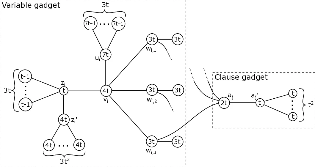
NP‑hardness on planar graphs
The core hardness result is proved by a polynomial‑time reduction from Cubic Planar Monotone 1‑in‑3 SAT, a known NP‑complete problem. For each variable and clause the construction introduces a “variable gadget” and a “clause gadget”, parameterised by an integer t ≥ 1. The gadgets contain many auxiliary vertices (leaves) with carefully chosen weights that force any feasible subgraph to retain certain edges (to avoid isolated vertices) while allowing a controlled choice that corresponds to setting a variable true or false. Lemmas establish tight bounds on the contribution of leaves to the penalty term, on the minimum possible sum of logarithms of degrees, and on the maximum possible sum when all edges are kept. By selecting t appropriately, the authors ensure that a satisfying assignment of the SAT instance exists if and only if there is a feasible subgraph whose score exceeds a specific threshold. Consequently, even when the input graph is planar, the optimisation problem cannot be solved in polynomial time unless P = NP.

Two simplified variants
The paper also analyses two restricted versions of the problem.

1. Zero‑penalty variant: The task is to find a spanning subgraph with ND_H(v,f) = 0 for every vertex (i.e., the penalty term vanishes). The authors completely characterise such subgraphs and present a linear‑time algorithm (O(|E|)) that constructs an optimal solution by simply preserving all edges incident to leaves and ensuring each internal vertex’s neighbours have matching average weight.
2. Zero‑penalty on high‑degree vertices: When the requirement that ND_H(v,f) = 0 is imposed only on vertices of degree at least two, the problem remains NP‑complete. This demonstrates that even modest relaxations do not reduce the inherent difficulty.

Exact parameterised algorithms
Despite the hardness, the authors provide two exact algorithms that are efficient under realistic restrictions often met in spatial applications.

1. Tree‑decomposition based dynamic programming

   • Parameters: treewidth tw(G) and maximum degree Δ(G).
   • Pre‑computation: f(tw,Δ)·n^{O(Δ)} time, where f is exponential only in the parameters.
   • Delay: linear in n between successive outputs.
   • Post‑processing: linear time.
     The algorithm builds a nice tree decomposition of G, then processes bags bottom‑up, storing for each bag a table of partial solutions that respect degree constraints and keep track of the penalty contributions. Because the degree bound limits the number of possible neighbour‑sets per vertex, the table size remains polynomial when Δ is constant. This yields both a decision procedure (does a subgraph with score ≥ K exist?) and an enumeration of all optimal subgraphs.

2. Maximum‑degree‑three, edge‑deletion‑budget parameterisation

   • Assumption: the input graph has Δ(G) ≤ 3, which is typical for triangulations of planar regions.
   • Parameter: k, the maximum number of edges that may be removed.
   • Pre‑computation: f(k)·n·log n time (fixed‑parameter tractable).
   • Delay: O(1) (linear) between outputs.
     The method enumerates all subsets of at most k edges, but prunes aggressively using structural properties of degree‑three graphs (e.g., each removal creates a small “defect” that can be propagated locally). It then checks feasibility (no isolated vertices) and computes the score. Because k is often small in practice (only a few edges need to be removed to improve model fit), the algorithm is practical and, crucially, returns every optimal subgraph.

Both algorithms output not just a single optimal configuration but the entire solution space. This is valuable for Bayesian spatial modelling: the set of optimal graphs can be treated as a discrete prior or used to quantify uncertainty about the neighbourhood structure, leading to more robust inference for conditional autoregressive (CAR) models.

Broader implications and future work
The paper highlights that estimating the neighbourhood matrix (graph) should be treated as a genuine statistical parameter rather than a fixed design choice. By providing exact enumeration tools, the authors enable practitioners to propagate graph‑selection uncertainty through downstream analyses. Open directions include: (i) designing approximation schemes for graphs with large treewidth or high degree, (ii) extending the framework to dynamic settings where vertex weights evolve over time, and (iii) integrating the optimisation into hierarchical Bayesian models where the score function appears as a log‑likelihood component. Overall, the work bridges a gap between theoretical computer science (complexity, parameterised algorithms) and spatial statistics, offering both hardness insights and practical algorithms for a problem that previously relied on heuristics.