Bio-Inspired Hashing for Unsupervised Similarity Search

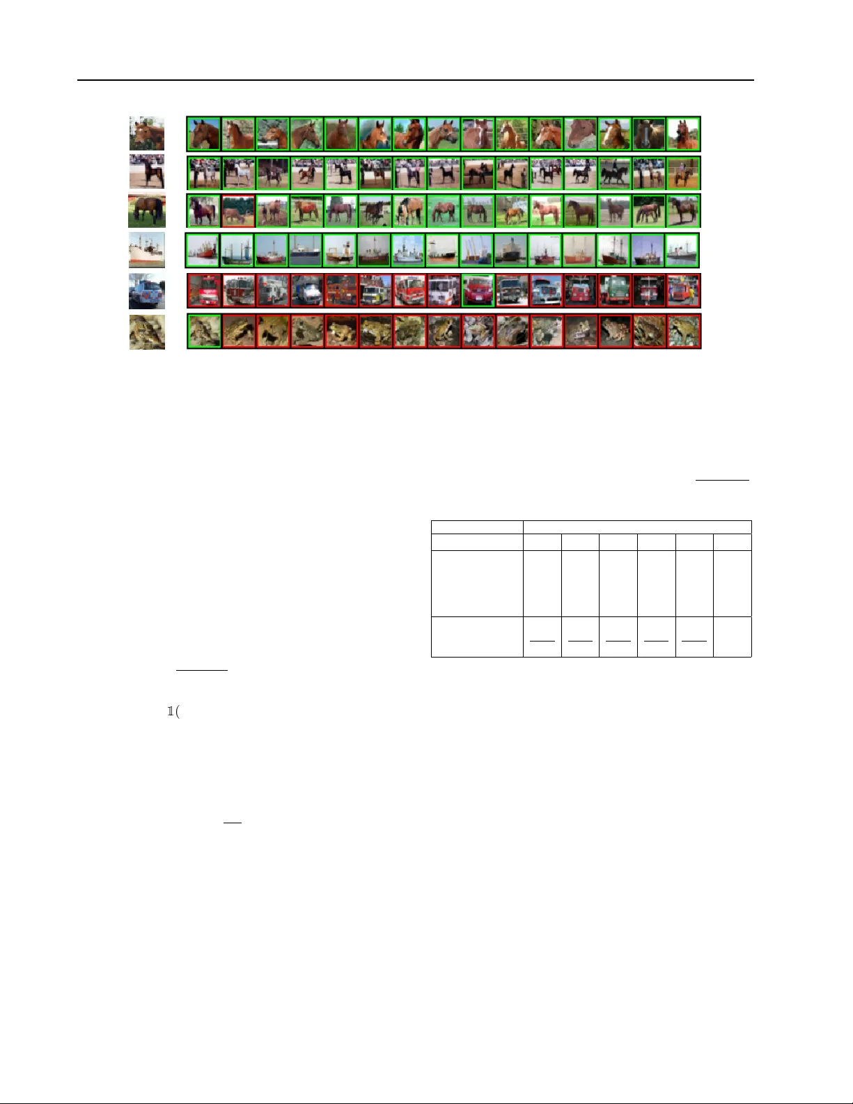
Bio-Inspir ed Hashing f or Unsupervised Similarity Sear ch Chaitanya K. Ryali 1 2 John J . Hopﬁeld 3 Leopold Grinberg 4 Dmitry Kroto v 2 4 Abstract The fruit ﬂy Drosophila’ s olfactory circuit has inspired a new locality sensitive hashing (LSH) algorithm, FlyHash . In contrast with classical LSH algorithms that produce low dimensional hash codes, FlyHash produces sparse high- dimensional hash codes and has also been shown to ha ve superior empirical performance compared to classical LSH algorithms in similarity search. Ho wev er , FlyHash uses random projections and cannot learn from data. Building on inspiration from FlyHash and the ubiquity of sparse e xpan- siv e representations in neurobiology , our work proposes a nov el hashing algorithm BioHash that produces sparse high dimensional hash codes in a data-driven manner . W e sho w that BioHash outperforms previously published benchmarks for various hashing methods. Since our learn- ing algorithm is based on a local and biologically plausible synaptic plasticity rule, our work pro- vides e vidence for the proposal that LSH might be a computational reason for the abundance of sparse expansi ve motifs in a variety of biological systems. W e also propose a conv olutional v ari- ant BioConvHash that further improv es perfor - mance. From the perspecti ve of computer science, BioHash and BioConvHash are fast, scalable and yield compressed binary representations that are useful for similarity search. 1. Introduction Sparse expansi ve representations are ubiquitous in neuro- biology . Expansion means that a high-dimensional input is mapped to an ev en higher dimensional secondary rep- resentation. Such expansion is often accompanied by a sparsiﬁcation of the activ ations: dense input data is mapped 1 Department of CS and Engineering, UC San Diego 2 MIT - IBM W atson AI Lab 3 Princeton Neuroscience Institute, Princeton Univ ersity 4 IBM Research. Correspondence to: C.K. Ryali , D. Krotov . Pr oceedings of the 37 th International Conference on Machine Learning , V ienna, Austria, PMLR 119, 2020. Cop yright 2020 by the author(s). into a sparse code, where only a small number of secondary neurons respond to a giv en stimulus. A classical example of the sparse expansi ve motif is the Drosophila fruit ﬂy olfactory system. In this case, approxi- mately 50 projection neurons send their acti vities to about 2500 Ken yon cells ( T urner et al. , 2008 ), thus accomplishing an approximately 50 x expansion. An input stimulus typ- ically activ ates approximately 50% of projection neurons, and less than 10% Ken yon cells ( T urner et al. , 2008 ), provid- ing an example of signiﬁcant sparsiﬁcation of the expanded codes. Another example is the rodent olfactory circuit. In this system, dense input from the olfactory b ulb is projected into piriform cortex, which has 1000 x more neurons than the number of glomeruli in the olfactory bulb . Only about 10% of those neurons respond to a giv en stimulus ( Mombaerts et al. , 1996 ). A similar motif is found in rat’ s cerebellum and hippocampus ( Dasgupta et al. , 2017 ). From the computational perspectiv e, expansion is helpful for increasing the number of classiﬁcation decision bound- aries by a simple perceptron ( Cov er , 1965 ) or increasing memory storage capacity in models of associati ve memory ( Hopﬁeld , 1982 ). Additionally , sparse expansi ve represen- tations hav e been shown to reduce intrastimulus v ariability and the overlaps between representations induced by dis- tinct stimuli ( Sompolinsk y , 2014 ). Sparseness has also been shown to increase the capacity of models of associative memory ( Tsodyks & Feigelman , 1988 ). The goal of our work is to use this “biological” inspiration about sparse expansiv e motifs, as well as local Hebbian learning, for designing a nov el hashing algorithm BioHash that can be used in similarity search. W e describe the task, the algorithm, and demonstrate that BioHash improv es retriev al performance on common benchmarks. Similarity search and LSH. In similarity search, gi ven a query q ∈ R d , a similarity measure sim ( q , x ) , and a database X ∈ R n × d containing n items, the objectiv e is to retriev e a ranked list of R items from the database most similar to q . When data is high-dimensional (e.g. im- ages/documents) and the databases are lar ge (millions or bil- lions items), this is a computationally challenging problem. Howe ver , approximate solutions are generally acceptable, with Locality Sensiti ve Hashing (LSH) being one such ap- proach ( W ang et al. , 2014 ). Similarity search approaches Bio-Inspired Hashing f or Unsupervised Similarity Search m ⌧ d AAAB7XicbVDLSgNBEOyNrxhfUY9eBoPgKeyKoMegF48RzAOSJczOziZj5rHMzAphyT948aCIV//Hm3/jJNmDJhY0FFXddHdFKWfG+v63V1pb39jcKm9Xdnb39g+qh0dtozJNaIsornQ3woZyJmnLMstpN9UUi4jTTjS+nfmdJ6oNU/LBTlIaCjyULGEEWye1RZ9zFA+qNb/uz4FWSVCQGhRoDqpf/ViRTFBpCcfG9AI/tWGOtWWE02mlnxmaYjLGQ9pzVGJBTZjPr52iM6fEKFHalbRorv6eyLEwZiIi1ymwHZllbyb+5/Uym1yHOZNpZqkki0VJxpFVaPY6ipmmxPKJI5ho5m5FZIQ1JtYFVHEhBMsvr5L2RT3w68H9Za1xU8RRhhM4hXMI4AoacAdNaAGBR3iGV3jzlPfivXsfi9aSV8wcwx94nz8u/o7b AAAB7XicbVDLSgNBEOyNrxhfUY9eBoPgKeyKoMegF48RzAOSJczOziZj5rHMzAphyT948aCIV//Hm3/jJNmDJhY0FFXddHdFKWfG+v63V1pb39jcKm9Xdnb39g+qh0dtozJNaIsornQ3woZyJmnLMstpN9UUi4jTTjS+nfmdJ6oNU/LBTlIaCjyULGEEWye1RZ9zFA+qNb/uz4FWSVCQGhRoDqpf/ViRTFBpCcfG9AI/tWGOtWWE02mlnxmaYjLGQ9pzVGJBTZjPr52iM6fEKFHalbRorv6eyLEwZiIi1ymwHZllbyb+5/Uym1yHOZNpZqkki0VJxpFVaPY6ipmmxPKJI5ho5m5FZIQ1JtYFVHEhBMsvr5L2RT3w68H9Za1xU8RRhhM4hXMI4AoacAdNaAGBR3iGV3jzlPfivXsfi9aSV8wcwx94nz8u/o7b AAAB7XicbVDLSgNBEOyNrxhfUY9eBoPgKeyKoMegF48RzAOSJczOziZj5rHMzAphyT948aCIV//Hm3/jJNmDJhY0FFXddHdFKWfG+v63V1pb39jcKm9Xdnb39g+qh0dtozJNaIsornQ3woZyJmnLMstpN9UUi4jTTjS+nfmdJ6oNU/LBTlIaCjyULGEEWye1RZ9zFA+qNb/uz4FWSVCQGhRoDqpf/ViRTFBpCcfG9AI/tWGOtWWE02mlnxmaYjLGQ9pzVGJBTZjPr52iM6fEKFHalbRorv6eyLEwZiIi1ymwHZllbyb+5/Uym1yHOZNpZqkki0VJxpFVaPY6ipmmxPKJI5ho5m5FZIQ1JtYFVHEhBMsvr5L2RT3w68H9Za1xU8RRhhM4hXMI4AoacAdNaAGBR3iGV3jzlPfivXsfi9aSV8wcwx94nz8u/o7b AAAB7XicbVDLSgNBEOyNrxhfUY9eBoPgKeyKoMegF48RzAOSJczOziZj5rHMzAphyT948aCIV//Hm3/jJNmDJhY0FFXddHdFKWfG+v63V1pb39jcKm9Xdnb39g+qh0dtozJNaIsornQ3woZyJmnLMstpN9UUi4jTTjS+nfmdJ6oNU/LBTlIaCjyULGEEWye1RZ9zFA+qNb/uz4FWSVCQGhRoDqpf/ViRTFBpCcfG9AI/tWGOtWWE02mlnxmaYjLGQ9pzVGJBTZjPr52iM6fEKFHalbRorv6eyLEwZiIi1ymwHZllbyb+5/Uym1yHOZNpZqkki0VJxpFVaPY6ipmmxPKJI5ho5m5FZIQ1JtYFVHEhBMsvr5L2RT3w68H9Za1xU8RRhhM4hXMI4AoacAdNaAGBR3iGV3jzlPfivXsfi9aSV8wcwx94nz8u/o7b m  d AAAB7XicbVDLSgNBEOyNrxhfUY9eBoPgKeyKoMegF48RzAOSJczOzm7GzGOZmRVCyD948aCIV//Hm3/jJNmDJhY0FFXddHdFGWfG+v63V1pb39jcKm9Xdnb39g+qh0dto3JNaIsornQ3woZyJmnLMstpN9MUi4jTTjS6nfmdJ6oNU/LBjjMaCpxKljCCrZPaop+mKB5Ua37dnwOtkqAgNSjQHFS/+rEiuaDSEo6N6QV+ZsMJ1pYRTqeVfm5ohskIp7TnqMSCmnAyv3aKzpwSo0RpV9Kiufp7YoKFMWMRuU6B7dAsezPxP6+X2+Q6nDCZ5ZZKsliU5BxZhWavo5hpSiwfO4KJZu5WRIZYY2JdQBUXQrD88ippX9QDvx7cX9YaN0UcZTiBUziHAK6gAXfQhBYQeIRneIU3T3kv3rv3sWgtecXMMfyB9/kDH72O0Q== AAAB7XicbVDLSgNBEOyNrxhfUY9eBoPgKeyKoMegF48RzAOSJczOzm7GzGOZmRVCyD948aCIV//Hm3/jJNmDJhY0FFXddHdFGWfG+v63V1pb39jcKm9Xdnb39g+qh0dto3JNaIsornQ3woZyJmnLMstpN9MUi4jTTjS6nfmdJ6oNU/LBjjMaCpxKljCCrZPaop+mKB5Ua37dnwOtkqAgNSjQHFS/+rEiuaDSEo6N6QV+ZsMJ1pYRTqeVfm5ohskIp7TnqMSCmnAyv3aKzpwSo0RpV9Kiufp7YoKFMWMRuU6B7dAsezPxP6+X2+Q6nDCZ5ZZKsliU5BxZhWavo5hpSiwfO4KJZu5WRIZYY2JdQBUXQrD88ippX9QDvx7cX9YaN0UcZTiBUziHAK6gAXfQhBYQeIRneIU3T3kv3rv3sWgtecXMMfyB9/kDH72O0Q== AAAB7XicbVDLSgNBEOyNrxhfUY9eBoPgKeyKoMegF48RzAOSJczOzm7GzGOZmRVCyD948aCIV//Hm3/jJNmDJhY0FFXddHdFGWfG+v63V1pb39jcKm9Xdnb39g+qh0dto3JNaIsornQ3woZyJmnLMstpN9MUi4jTTjS6nfmdJ6oNU/LBjjMaCpxKljCCrZPaop+mKB5Ua37dnwOtkqAgNSjQHFS/+rEiuaDSEo6N6QV+ZsMJ1pYRTqeVfm5ohskIp7TnqMSCmnAyv3aKzpwSo0RpV9Kiufp7YoKFMWMRuU6B7dAsezPxP6+X2+Q6nDCZ5ZZKsliU5BxZhWavo5hpSiwfO4KJZu5WRIZYY2JdQBUXQrD88ippX9QDvx7cX9YaN0UcZTiBUziHAK6gAXfQhBYQeIRneIU3T3kv3rv3sWgtecXMMfyB9/kDH72O0Q== AAAB7XicbVDLSgNBEOyNrxhfUY9eBoPgKeyKoMegF48RzAOSJczOzm7GzGOZmRVCyD948aCIV//Hm3/jJNmDJhY0FFXddHdFGWfG+v63V1pb39jcKm9Xdnb39g+qh0dto3JNaIsornQ3woZyJmnLMstpN9MUi4jTTjS6nfmdJ6oNU/LBjjMaCpxKljCCrZPaop+mKB5Ua37dnwOtkqAgNSjQHFS/+rEiuaDSEo6N6QV+ZsMJ1pYRTqeVfm5ohskIp7TnqMSCmnAyv3aKzpwSo0RpV9Kiufp7YoKFMWMRuU6B7dAsezPxP6+X2+Q6nDCZ5ZZKsliU5BxZhWavo5hpSiwfO4KJZu5WRIZYY2JdQBUXQrD88ippX9QDvx7cX9YaN0UcZTiBUziHAK6gAXfQhBYQeIRneIU3T3kv3rv3sWgtecXMMfyB9/kDH72O0Q== W AAAB8XicbVDLSsNAFL2pr1pfVZduBovgqiQi6LLoxmUF+8A2lMl00g6dTMLMjVBC/8KNC0Xc+jfu/BsnbRbaemDgcM69zLknSKQw6LrfTmltfWNzq7xd2dnd2z+oHh61TZxqxlsslrHuBtRwKRRvoUDJu4nmNAok7wST29zvPHFtRKwecJpwP6IjJULBKFrpsR9RHAdh1pkNqjW37s5BVolXkBoUaA6qX/1hzNKIK2SSGtPz3AT9jGoUTPJZpZ8anlA2oSPes1TRiBs/myeekTOrDEkYa/sUkrn6eyOjkTHTKLCTeUKz7OXif14vxfDaz4RKUuSKLT4KU0kwJvn5ZCg0ZyinllCmhc1K2JhqytCWVLEleMsnr5L2Rd1z6979Za1xU9RRhhM4hXPw4AoacAdNaAEDBc/wCm+OcV6cd+djMVpyip1j+APn8wfLFJD7 AAAB8XicbVDLSsNAFL2pr1pfVZduBovgqiQi6LLoxmUF+8A2lMl00g6dTMLMjVBC/8KNC0Xc+jfu/BsnbRbaemDgcM69zLknSKQw6LrfTmltfWNzq7xd2dnd2z+oHh61TZxqxlsslrHuBtRwKRRvoUDJu4nmNAok7wST29zvPHFtRKwecJpwP6IjJULBKFrpsR9RHAdh1pkNqjW37s5BVolXkBoUaA6qX/1hzNKIK2SSGtPz3AT9jGoUTPJZpZ8anlA2oSPes1TRiBs/myeekTOrDEkYa/sUkrn6eyOjkTHTKLCTeUKz7OXif14vxfDaz4RKUuSKLT4KU0kwJvn5ZCg0ZyinllCmhc1K2JhqytCWVLEleMsnr5L2Rd1z6979Za1xU9RRhhM4hXPw4AoacAdNaAEDBc/wCm+OcV6cd+djMVpyip1j+APn8wfLFJD7 AAAB8XicbVDLSsNAFL2pr1pfVZduBovgqiQi6LLoxmUF+8A2lMl00g6dTMLMjVBC/8KNC0Xc+jfu/BsnbRbaemDgcM69zLknSKQw6LrfTmltfWNzq7xd2dnd2z+oHh61TZxqxlsslrHuBtRwKRRvoUDJu4nmNAok7wST29zvPHFtRKwecJpwP6IjJULBKFrpsR9RHAdh1pkNqjW37s5BVolXkBoUaA6qX/1hzNKIK2SSGtPz3AT9jGoUTPJZpZ8anlA2oSPes1TRiBs/myeekTOrDEkYa/sUkrn6eyOjkTHTKLCTeUKz7OXif14vxfDaz4RKUuSKLT4KU0kwJvn5ZCg0ZyinllCmhc1K2JhqytCWVLEleMsnr5L2Rd1z6979Za1xU9RRhhM4hXPw4AoacAdNaAEDBc/wCm+OcV6cd+djMVpyip1j+APn8wfLFJD7 AAAB8XicbVDLSsNAFL2pr1pfVZduBovgqiQi6LLoxmUF+8A2lMl00g6dTMLMjVBC/8KNC0Xc+jfu/BsnbRbaemDgcM69zLknSKQw6LrfTmltfWNzq7xd2dnd2z+oHh61TZxqxlsslrHuBtRwKRRvoUDJu4nmNAok7wST29zvPHFtRKwecJpwP6IjJULBKFrpsR9RHAdh1pkNqjW37s5BVolXkBoUaA6qX/1hzNKIK2SSGtPz3AT9jGoUTPJZpZ8anlA2oSPes1TRiBs/myeekTOrDEkYa/sUkrn6eyOjkTHTKLCTeUKz7OXif14vxfDaz4RKUuSKLT4KU0kwJvn5ZCg0ZyinllCmhc1K2JhqytCWVLEleMsnr5L2Rd1z6979Za1xU9RRhhM4hXPw4AoacAdNaAEDBc/wCm+OcV6cd+djMVpyip1j+APn8wfLFJD7 W AAAB8XicbVDLSsNAFL2pr1pfVZduBovgqiQi6LLoxmUF+8A2lMl00g6dTMLMjVBC/8KNC0Xc+jfu/BsnbRbaemDgcM69zLknSKQw6LrfTmltfWNzq7xd2dnd2z+oHh61TZxqxlsslrHuBtRwKRRvoUDJu4nmNAok7wST29zvPHFtRKwecJpwP6IjJULBKFrpsR9RHAdh1pkNqjW37s5BVolXkBoUaA6qX/1hzNKIK2SSGtPz3AT9jGoUTPJZpZ8anlA2oSPes1TRiBs/myeekTOrDEkYa/sUkrn6eyOjkTHTKLCTeUKz7OXif14vxfDaz4RKUuSKLT4KU0kwJvn5ZCg0ZyinllCmhc1K2JhqytCWVLEleMsnr5L2Rd1z6979Za1xU9RRhhM4hXPw4AoacAdNaAEDBc/wCm+OcV6cd+djMVpyip1j+APn8wfLFJD7 AAAB8XicbVDLSsNAFL2pr1pfVZduBovgqiQi6LLoxmUF+8A2lMl00g6dTMLMjVBC/8KNC0Xc+jfu/BsnbRbaemDgcM69zLknSKQw6LrfTmltfWNzq7xd2dnd2z+oHh61TZxqxlsslrHuBtRwKRRvoUDJu4nmNAok7wST29zvPHFtRKwecJpwP6IjJULBKFrpsR9RHAdh1pkNqjW37s5BVolXkBoUaA6qX/1hzNKIK2SSGtPz3AT9jGoUTPJZpZ8anlA2oSPes1TRiBs/myeekTOrDEkYa/sUkrn6eyOjkTHTKLCTeUKz7OXif14vxfDaz4RKUuSKLT4KU0kwJvn5ZCg0ZyinllCmhc1K2JhqytCWVLEleMsnr5L2Rd1z6979Za1xU9RRhhM4hXPw4AoacAdNaAEDBc/wCm+OcV6cd+djMVpyip1j+APn8wfLFJD7 AAAB8XicbVDLSsNAFL2pr1pfVZduBovgqiQi6LLoxmUF+8A2lMl00g6dTMLMjVBC/8KNC0Xc+jfu/BsnbRbaemDgcM69zLknSKQw6LrfTmltfWNzq7xd2dnd2z+oHh61TZxqxlsslrHuBtRwKRRvoUDJu4nmNAok7wST29zvPHFtRKwecJpwP6IjJULBKFrpsR9RHAdh1pkNqjW37s5BVolXkBoUaA6qX/1hzNKIK2SSGtPz3AT9jGoUTPJZpZ8anlA2oSPes1TRiBs/myeekTOrDEkYa/sUkrn6eyOjkTHTKLCTeUKz7OXif14vxfDaz4RKUuSKLT4KU0kwJvn5ZCg0ZyinllCmhc1K2JhqytCWVLEleMsnr5L2Rd1z6979Za1xU9RRhhM4hXPw4AoacAdNaAEDBc/wCm+OcV6cd+djMVpyip1j+APn8wfLFJD7 AAAB8XicbVDLSsNAFL2pr1pfVZduBovgqiQi6LLoxmUF+8A2lMl00g6dTMLMjVBC/8KNC0Xc+jfu/BsnbRbaemDgcM69zLknSKQw6LrfTmltfWNzq7xd2dnd2z+oHh61TZxqxlsslrHuBtRwKRRvoUDJu4nmNAok7wST29zvPHFtRKwecJpwP6IjJULBKFrpsR9RHAdh1pkNqjW37s5BVolXkBoUaA6qX/1hzNKIK2SSGtPz3AT9jGoUTPJZpZ8anlA2oSPes1TRiBs/myeekTOrDEkYa/sUkrn6eyOjkTHTKLCTeUKz7OXif14vxfDaz4RKUuSKLT4KU0kwJvn5ZCg0ZyinllCmhc1K2JhqytCWVLEleMsnr5L2Rd1z6979Za1xU9RRhhM4hXPw4AoacAdNaAEDBc/wCm+OcV6cd+djMVpyip1j+APn8wfLFJD7 k active neurons AAACAXicbVDLSgNBEJyNrxhfUS+Cl8EgeAq7Iugx6MVjBPOA7BJmJ51kyOzsMtMbDEu8+CtePCji1b/w5t84eRw0saChqOqmuytMpDDout9ObmV1bX0jv1nY2t7Z3SvuH9RNnGoONR7LWDdDZkAKBTUUKKGZaGBRKKERDm4mfmMI2ohY3eMogSBiPSW6gjO0Urt4NPARHjDzKeMohkAVpDpWZtwultyyOwVdJt6clMgc1Xbxy+/EPI1AIZfMmJbnJhhkTKPgEsYFPzWQMD5gPWhZqlgEJsimH4zpqVU6tBtrWwrpVP09kbHImFEU2s6IYd8sehPxP6+VYvcqyIRKUgTFZ4u6qaQY00kctCM0cJQjSxjXwt5KeZ9pG4YNrWBD8BZfXib187Lnlr27i1Lleh5HnhyTE3JGPHJJKuSWVEmNcPJInskreXOenBfn3fmYteac+cwh+QPn8wcJlpdB AAACAXicbVDLSgNBEJyNrxhfUS+Cl8EgeAq7Iugx6MVjBPOA7BJmJ51kyOzsMtMbDEu8+CtePCji1b/w5t84eRw0saChqOqmuytMpDDout9ObmV1bX0jv1nY2t7Z3SvuH9RNnGoONR7LWDdDZkAKBTUUKKGZaGBRKKERDm4mfmMI2ohY3eMogSBiPSW6gjO0Urt4NPARHjDzKeMohkAVpDpWZtwultyyOwVdJt6clMgc1Xbxy+/EPI1AIZfMmJbnJhhkTKPgEsYFPzWQMD5gPWhZqlgEJsimH4zpqVU6tBtrWwrpVP09kbHImFEU2s6IYd8sehPxP6+VYvcqyIRKUgTFZ4u6qaQY00kctCM0cJQjSxjXwt5KeZ9pG4YNrWBD8BZfXib187Lnlr27i1Lleh5HnhyTE3JGPHJJKuSWVEmNcPJInskreXOenBfn3fmYteac+cwh+QPn8wcJlpdB AAACAXicbVDLSgNBEJyNrxhfUS+Cl8EgeAq7Iugx6MVjBPOA7BJmJ51kyOzsMtMbDEu8+CtePCji1b/w5t84eRw0saChqOqmuytMpDDout9ObmV1bX0jv1nY2t7Z3SvuH9RNnGoONR7LWDdDZkAKBTUUKKGZaGBRKKERDm4mfmMI2ohY3eMogSBiPSW6gjO0Urt4NPARHjDzKeMohkAVpDpWZtwultyyOwVdJt6clMgc1Xbxy+/EPI1AIZfMmJbnJhhkTKPgEsYFPzWQMD5gPWhZqlgEJsimH4zpqVU6tBtrWwrpVP09kbHImFEU2s6IYd8sehPxP6+VYvcqyIRKUgTFZ4u6qaQY00kctCM0cJQjSxjXwt5KeZ9pG4YNrWBD8BZfXib187Lnlr27i1Lleh5HnhyTE3JGPHJJKuSWVEmNcPJInskreXOenBfn3fmYteac+cwh+QPn8wcJlpdB AAACAXicbVDLSgNBEJyNrxhfUS+Cl8EgeAq7Iugx6MVjBPOA7BJmJ51kyOzsMtMbDEu8+CtePCji1b/w5t84eRw0saChqOqmuytMpDDout9ObmV1bX0jv1nY2t7Z3SvuH9RNnGoONR7LWDdDZkAKBTUUKKGZaGBRKKERDm4mfmMI2ohY3eMogSBiPSW6gjO0Urt4NPARHjDzKeMohkAVpDpWZtwultyyOwVdJt6clMgc1Xbxy+/EPI1AIZfMmJbnJhhkTKPgEsYFPzWQMD5gPWhZqlgEJsimH4zpqVU6tBtrWwrpVP09kbHImFEU2s6IYd8sehPxP6+VYvcqyIRKUgTFZ4u6qaQY00kctCM0cJQjSxjXwt5KeZ9pG4YNrWBD8BZfXib187Lnlr27i1Lleh5HnhyTE3JGPHJJKuSWVEmNcPJInskreXOenBfn3fmYteac+cwh+QPn8wcJlpdB Figure 1. Hashing algorithms use either representational contraction (large dimension of input is mapped into a smaller dimensional latent space), or expansion (lar ge dimensional input is mapped into an ev en larger dimensional latent space). The projections can be random or data driv en. maybe unsupervised or supervised. Since labelled informa- tion for extremely lar ge datasets is infeasible to obtain, our work focuses on the unsupervised setting. In LSH ( Indyk & Motwani , 1998 ; Charikar , 2002 ), the idea is to encode each database entry x (and query q ) with a binary representation h ( x ) ( h ( q ) respecti vely) and to retrieve R entries with small- est Hamming distances d H ( h ( x ) , h ( q )) . Intuitiv ely , (see ( Charikar , 2002 ), for a formal deﬁnition), a hash function h : R d − → {− 1 , 1 } m is said to be locality sensitive , if simi- lar (dissimilar) items x 1 and x 2 are close by (far apart) in Hamming distance d H ( h ( x 1 ) , h ( x 2 )) . LSH algorithms are of fundamental importance in computer science, with appli- cations in similarity search, data compression and machine learning ( Andoni & Indyk , 2008 ). In the similarity search literature, two distinct settings are generally considered: a) descriptors (e.g. SIFT , GIST) are assumed to be given and the ground truth is based on a measure of similarity in descriptor space ( W eiss et al. , 2009 ; Sharma & Navlakha , 2018 ; Jégou et al. , 2011 ) and b) descriptors are learned and the similarity measure is based on semantic labels ( Lin et al. , 2013 ; Jin et al. , 2019 ; Do et al. , 2017b ; Su et al. , 2018 ). This current work is closer to the latter setting. Our approach is unsupervised, the labels are only used for ev aluation. Drosophila olfactory circuit and FlyHash. In classical LSH approaches, the data dimensionality d is much larger than the embedding space dimension m , resulting in low- dimensional hash codes ( W ang et al. , 2014 ; Indyk & Mot- wani , 1998 ; Charikar , 2002 ). In contrast, a new family of hashing algorithms has been proposed ( Dasgupta et al. , 2017 ) where m  d , but the secondary representation is highly sparse with only a small number k of m units being activ e, see Figure 1 . W e call this algorithm FlyHash in this paper , since it is motiv ated by the computation carried out by the ﬂy’ s olfactory circuit. The expansion from the d dimensional input space into an m dimensional secondary representation is carried out using a random set of weights W ( Dasgupta et al. , 2017 ; Caron et al. , 2013 ). The resulting high dimensional representation is sparsiﬁed by k -W inner- T ake-All ( k -WT A) feedback inhibition in the hidden layer resulting in top ∼ 5% of units staying activ e ( Lin et al. , 2014 ; Stev ens , 2016 ). While FlyHash uses random synaptic weights, sparse ex- pansiv e representations are not necessarily random ( Som- polinsky , 2014 ), perhaps not e ven in the case of Drosophila ( Gruntman & T urner , 2013 ; Zheng et al. , 2018 ). More- ov er, using synaptic weights that are learned from data might help to further impro ve the locality sensiti vity prop- erty of FlyHash . Thus, it is important to in vestigate the role of learned synapses on the hashing performance. A recent work SOLHash ( Li et al. , 2018 ), takes inspira- tion from FlyHash and attempts to adapt the synapses to data, demonstrating improved performance o ver FlyHash . Howe ver , ev ery learning update step in SOLHash in vokes a constrained linear program and also requires computing pairwise inner-products between all training points, making it very time consuming and limiting its scalability to datasets of ev en modest size. These limitations restrict SOLHash to training only on a small fraction of the data ( Li et al. , 2018 ). Additionally , SOLHash is biologically implausible (an ex- tended discussion is included in the supplementary informa- tion). BioHash also takes inspiration from FlyHash and demonstrates improv ed performance compared to random weights used in FlyHash , but it is fast, online, scalable and, importantly , BioHash is neurobiologically plausible. Not only "biological" inspiration can lead to improving hash- ing techniques, but the opposite might also be true. One of the statements of the present paper is that BioHash satisﬁes locality sensitiv e property , and, at the same time, utilizes a biologically plausible learning rule for synaptic weights ( Krotov & Hopﬁeld , 2019 ). This provides e vidence tow ard the proposal that the reason why sparse expansiv e representations are so common in biological or ganisms is because they perform locality sensitiv e hashing. In other words, they cluster similar stimuli together and push distinct stimuli far apart. Thus, our work provides e vidence tow ard the proposal that LSH might be a fundamental computa- tional principle utilized by the sparse expansiv e circuits Fig. 1 (right). Importantly , learning of synapses must be biologi- cally plausible (the synaptic plasticity rule should be local). Contributions. Building on inspiration from FlyHash and more broadly the ubiquity of sparse, expansiv e rep- resentations in neurobiology , our work proposes a novel hashing algorithm BioHash , that in contrast with previ- ous work ( Dasgupta et al. , 2017 ; Li et al. , 2018 ), produces Bio-Inspired Hashing f or Unsupervised Similarity Search sparse high dimensional hash codes in a data-driven manner and with learning of synapses in a neur obiologically plau- sible way . W e provide an existence proof for the proposal that LSH maybe a fundamental computational principle in neural circuits ( Dasgupta et al. , 2017 ) in the context of learned synapses. W e incorporate con volutional structure into BioHash , resulting in improv ed performance and ro- bustness to v ariations in intensity . From the perspecti ve of computer science, we sho w that BioHash is simple, scal- able to large datasets and demonstrates good performance for similarity search. Interestingly , BioHash outperforms a number of recent state-of-the-art deep hashing methods trained via backpropogation. 2. A pproximate Similarity Search via BioHashing Formally , if we denote a data point as x ∈ R d , we seek a binary hash code y ∈ {− 1 , 1 } m . W e deﬁne the hash length of a binary code as k , if the exact Hamming distance computation is O ( k ) . Below we present our bio-inspired hashing algorithm. 2.1. Bio-inspired Hashing (BioHash) W e adopt a biologically plausible unsupervised algorithm for representation learning from ( Krotov & Hopﬁeld , 2019 ). Denote the synapses from the input layer to the hash layer as W ∈ R m × d . The learning dynamics for the synapses of an individual neuron µ , denoted by W µi , is giv en by τ dW µi dt = g h Rank  h W µ , x i µ  i x i − h W µ , x i µ W µi  , (1) where W µ = ( W µ 1 , W µ 2 ...W µd ) , and g [ µ ] =      1 , µ = 1 − ∆ , µ = r 0 , otherwise (2) and h x, y i µ = P i,j η µ i,j x i y j , with η µ i,j = | W µi | p − 2 δ ij , where δ ij is Kronecker delta and τ is the time scale of the learning dynamics. The Rank operation in equation ( 1 ) sorts the inner products from the largest ( µ = 1 ) to the smallest ( µ = m ). The training dynamics can be shown to minimize the following ener gy function 1 E = − X A m X µ =1 g h Rank  h W µ , x A i µ  i h W µ , x A i µ h W µ , W µ i p − 1 p µ , (3) 1 Note that while ( Krotov & Hopﬁeld , 2019 ) analyzed a simi- lar energy function, it does not characterize the energy function corresponding to these learning dynamics ( 1 ) where A index es the training example. It can be shown that the synapses con ver ge to a unit ( p − norm) sphere ( Kroto v & Hopﬁeld , 2019 ). Note that the training dynamics do not perform gradient descent, i.e ˙ W µ 6 = ∇ W µ E . Howe ver , time deri vati ve of the ener gy function under dynamics ( 1 ) is always ne gativ e (we sho w this for the case ∆ = 0 belo w), τ dE dt = − X A τ ( p − 1) h W ˆ µ , W ˆ µ i p − 1 p +1 ˆ µ h h dW ˆ µ dt , x A i ˆ µ h W ˆ µ , W ˆ µ i ˆ µ −h W ˆ µ , x A i ˆ µ h dW ˆ µ dt , W ˆ µ i ˆ µ i = − X A τ ( p − 1) h W ˆ µ , W ˆ µ i p − 1 p +1 ˆ µ h h x A , x A i ˆ µ h W ˆ µ , W ˆ µ i ˆ µ −h W ˆ µ , x A i 2 ˆ µ i ≤ 0 , (4) where Cauchy-Schwartz inequality is used. For ev ery train- ing example A the index of the acti v ated hidden unit is deﬁned as ˆ µ = arg max µ  h W µ , x A i µ  . (5) Thus, the energy function decreases during learning. A similar result can be shown for ∆ 6 = 0 . For p = 2 and ∆ = 0 , the ener gy function ( 3 ) reduces to an online version of the familiar spherical K -means cluster- ing algorithm ( Dhillon & Modha , 2001 ). In this limit, our learning rule can be considered an online and biologically plausible realization of this commonly used method. The hyperparameters p and ∆ provide additional ﬂexibility to our learning rule, compared to spherical K -means, while retaining biological plausibility . For instance, p = 1 can be set to induce sparsity in the synapses, as this would enforce || W µ || 1 = 1 . Empirically , we ﬁnd that general (non-zero) values of ∆ improv e the performance of our algorithm. After the learning-phase is complete, the hash code is gener - ated, as in FlyHash , via WT A sparsiﬁcation: for a given query x we generate a hash code y ∈ {− 1 , 1 } m as y µ = ( 1 , h W µ , x i µ is in top k − 1 , otherwise . (6) Thus, the hyperparameters of the method are p, r , m and ∆ . Note that the synapses are updated based only on pre- and post-synaptic activ ations resulting in Hebbian or anti- Hebbian updates. Many "unsupervised" learning to hash approaches provide a sort of "weak supervision" in the form of similarities ev aluated in the feature space of deep Con vo- lutional Neural Networks (CNNs) trained on ImageNet ( Jin et al. , 2019 ) to achiev e good performance. BioHash does not assume such information is provided and is completely unsupervised. Bio-Inspired Hashing f or Unsupervised Similarity Search - data point - inactive unit (-1) - active unit (+1) data probability density of the data A B x AAAB6HicbVDLTgJBEOzFF+IL9ehlIjHxRHbRRI9ELx4hkUcCGzI79MLI7OxmZtZICF/gxYPGePWTvPk3DrAHBSvppFLVne6uIBFcG9f9dnJr6xubW/ntws7u3v5B8fCoqeNUMWywWMSqHVCNgktsGG4EthOFNAoEtoLR7cxvPaLSPJb3ZpygH9GB5CFn1Fip/tQrltyyOwdZJV5GSpCh1it+dfsxSyOUhgmqdcdzE+NPqDKcCZwWuqnGhLIRHWDHUkkj1P5kfuiUnFmlT8JY2ZKGzNXfExMaaT2OAtsZUTPUy95M/M/rpCa89idcJqlByRaLwlQQE5PZ16TPFTIjxpZQpri9lbAhVZQZm03BhuAtv7xKmpWyd1Gu1C9L1ZssjjycwCmcgwdXUIU7qEEDGCA8wyu8OQ/Oi/PufCxac042cwx/4Hz+AOeHjQA= y 1 AAAB6nicbVBNS8NAEJ3Ur1q/qh69LBbBU0mqoMeiF48V7Qe0oWy2m3bpZhN2J0Io/QlePCji1V/kzX/jts1BWx8MPN6bYWZekEhh0HW/ncLa+sbmVnG7tLO7t39QPjxqmTjVjDdZLGPdCajhUijeRIGSdxLNaRRI3g7GtzO//cS1EbF6xCzhfkSHSoSCUbTSQ9b3+uWKW3XnIKvEy0kFcjT65a/eIGZpxBUySY3pem6C/oRqFEzyaamXGp5QNqZD3rVU0YgbfzI/dUrOrDIgYaxtKSRz9ffEhEbGZFFgOyOKI7PszcT/vG6K4bU/ESpJkSu2WBSmkmBMZn+TgdCcocwsoUwLeythI6opQ5tOyYbgLb+8Slq1qndRrd1fVuo3eRxFOIFTOAcPrqAOd9CAJjAYwjO8wpsjnRfn3flYtBacfOYY/sD5/AEOhI2l y 2 AAAB6nicbVBNS8NAEJ3Ur1q/qh69LBbBU0mqoMeiF48V7Qe0oWy2m3bpZhN2J0Io/QlePCji1V/kzX/jts1BWx8MPN6bYWZekEhh0HW/ncLa+sbmVnG7tLO7t39QPjxqmTjVjDdZLGPdCajhUijeRIGSdxLNaRRI3g7GtzO//cS1EbF6xCzhfkSHSoSCUbTSQ9av9csVt+rOQVaJl5MK5Gj0y1+9QczSiCtkkhrT9dwE/QnVKJjk01IvNTyhbEyHvGupohE3/mR+6pScWWVAwljbUkjm6u+JCY2MyaLAdkYUR2bZm4n/ed0Uw2t/IlSSIldssShMJcGYzP4mA6E5Q5lZQpkW9lbCRlRThjadkg3BW355lbRqVe+iWru/rNRv8jiKcAKncA4eXEEd7qABTWAwhGd4hTdHOi/Ou/OxaC04+cwx/IHz+QMQCI2m y 3 AAAB6nicbVBNS8NAEJ3Ur1q/qh69LBbBU0laQY9FLx4r2lpoQ9lsJ+3SzSbsboQS+hO8eFDEq7/Im//GbZuDtj4YeLw3w8y8IBFcG9f9dgpr6xubW8Xt0s7u3v5B+fCoreNUMWyxWMSqE1CNgktsGW4EdhKFNAoEPgbjm5n/+IRK81g+mEmCfkSHkoecUWOl+0m/3i9X3Ko7B1klXk4qkKPZL3/1BjFLI5SGCap113MT42dUGc4ETku9VGNC2ZgOsWuppBFqP5ufOiVnVhmQMFa2pCFz9fdERiOtJ1FgOyNqRnrZm4n/ed3UhFd+xmWSGpRssShMBTExmf1NBlwhM2JiCWWK21sJG1FFmbHplGwI3vLLq6Rdq3r1au3uotK4zuMowgmcwjl4cAkNuIUmtIDBEJ7hFd4c4bw4787HorXg5DPH8AfO5w8RjI2n Figure 2. (Panel A) Distribution of the hidden units (red circles) for a given distrib ution of the data (in one dimension). (Panel B) Arrangement of hidden units for the case of homogeneous distribution of the training data ρ = 1 / (2 π ) . For hash length k = 2 only two hidden units are acti vated (ﬁlled circles). If two data points are close to each other ( x and y 1 ) they elicit similar hash codes, if the tw o data points are far aw ay from each other ( x and y 3 ) - the hash codes are different. 2.2. Intuition An intuitiv e way to think about the learning algorithm is to view the hidden units as particles that are attracted to local peaks of the density of the data, and that simultaneously repel each other . T o demonstrate this, it is con venient to think about input data as randomly sampled points from a continuous distribution. Consider the case when p = 2 and ∆ = 0 . In this case, the energy function can be written as (since for p = 2 the inner product does not depend on the weights, we drop the subscript µ of the inner product) E = − 1 n X A h W ˆ µ , x A i h W ˆ µ , W ˆ µ i 1 2 = − Z Y i dv i 1 n X A δ ( v i − x A i ) h W ˆ µ , v i h W ˆ µ , W ˆ µ i 1 2 = − Z Y i dv i ρ ( v ) h W ˆ µ , v i h W ˆ µ , W ˆ µ i 1 2 , (7) where we introduced a continuous density of data ρ ( v ) . Furthermore, consider the case of d = 2 , and imagine that the data lies on a unit circle. In this case the density of data can be parametrized by a single angle ϕ . Thus, the energy function can be written as E = − π Z − π dϕρ ( ϕ ) cos( ϕ − ϕ ˆ µ ) , where ˆ µ = arg max µ  cos( ϕ − ϕ µ )  . (8) It is instructiv e to solve a simple case when the data follows an exponential distrib ution concentrated around zero angle with the decay length σ ( α is a normalization constant), ρ ( ϕ ) = αe − | ϕ | σ . (9) In this case, the energy ( 8 ) can be calculated exactly for any number of hidden units m . Howe ver , minimizing over the position of hidden units cannot be done analytically for general m . T o further simplify the problem consider the case when the number of hidden units m is small. For m = 2 the energy is equal to E = − α σ (1 + e − π σ ) 1 + σ 2  cos( ϕ 1 ) + σ sin( ϕ 1 )+ cos( ϕ 2 ) − σ sin( ϕ 2 )  . (10) Thus, in this simple case the energy is minimized when ϕ 1 , 2 = ± arctan( σ ) . (11) In the limit when the density of data is concentrated around zero angle ( σ → 0 ) the hidden units are attracted to the ori- gin and | ϕ 1 , 2 | ≈ σ . In the opposite limit ( σ → ∞ ) the data points are uniformly distributed on the circle. The resulting hidden units are then org anized to be on the opposite sides of the circle | ϕ 1 , 2 | = π 2 , due to mutual repulsion. Another limit when the problem can be solv ed analytically is the uniform density of the data ρ = 1 / (2 π ) for arbitrary number m of hidden units. In this case the hidden units span the entire circle homogeneously - the angle between two consecuti ve hidden units is ∆ ϕ = 2 π /m . These results are summarized in an intuitiv e cartoon in Fig- ure 2 , panel A. After learning is complete, the hidden units, denoted by circles, are localized in the vicinity of local max- ima of the probability density of the data. At the same time, repulsi ve force between the hidden units pre vents them from collapsing onto the exact position of the local maximum. Thus, the concentration of the hidden units near the local maxima becomes high, but, at the same time, they span the entire support (area where there is non-zero density) of the data distribution. For hashing purposes, trying to ﬁnd a data point x “closest” to some new query q requires a deﬁnition of “distance”. Since this measure is wanted only for nearby locations q and x , it need not be accurate for long distances. If we pick a set of m reference points in the space, then the loca- tion of point x can be speciﬁed by noting the few reference Bio-Inspired Hashing f or Unsupervised Similarity Search points it is closest to, producing a sparse and useful local representation. Uniformly tiling a high dimensional space is not a computationally useful approach. Reference points are needed only where there is data, and high resolution is needed only where there is high data density . The learning dynamics in ( 1 ) distributes m reference vectors by an itera- tiv e procedure such that their density is high where the data density is high, and low where the data density is lo w . This is exactly what is needed for a good hash code. The case of uniform density on a circle is illustrated in Figure 2 , panel B. After learning is complete the hidden units homogeneously span the entire circle. For hash length k = 2 , any giv en data point activ ates two closest hidden units. If two data points are located between two neigh- boring hidden units (like x and y 1 ) they produce exactly identical hash codes with hamming distance zero between them (black and red active units). If two data points are slightly f arther apart, like x and y 2 , the y produce hash codes that are slightly different (black and green circles, hamming distance is equal to 2 in this case). If the two data points are ev en farther , like x and y 3 , their hash codes are not overlap- ping at all (black and magenta circles, hamming distance is equal to 4 ). Thus, intuiti vely similar data acti vate similar hidden units, resulting in similar representations, while dis- similar data result in very dif f erent hash codes. As such, this intuition suggests that BioHash preferentially allocates representational capacity/resolution for local distances over global distances. W e verify this empirically in section 3.4 . 2.3. Computational Complexity and Metabolic Cost In classical LSH algorithms ( Charikar , 2002 ; Indyk & Mot- wani , 1998 ), typically , k = m and m  d , entailing a storage cost of k bits per database entry and O ( k ) compu- tational cost to compute Hamming distance. In BioHash (and in FlyHash ), typically m  k and m > d entailing storage cost of k log 2 m bits per database entry and O ( k ) 2 computational cost to compute Hamming distance. Note that while there is additional storage/lookup ov erhead over classical LSH in maintaining pointers, this is not unlike the storage/lookup ov erhead incurred by quantization methods like Product Quantization (PQ) ( Jégou et al. , 2011 ), which stores a lookup table of distances between ev ery pair of codew ords for each product space. From a neurobiologi- cal perspectiv e, a highly sparse representation such as the one produced by BioHash keeps the same metabolic cost ( Le vy & Baxter , 1996 ) as a dense low-dimensional ( m  d ) representation, such as in classical LSH methods. At the same time, as we empirically sho w belo w , it better preserv es similarity information. 2 If we maintain sorted pointers to the locations of 1 s, we hav e to compute the intersection between 2 ordered lists of length k , which is O ( k ) . T able 1. mAP@All (%) on MNIST (higher is better). Best re- sults (second best) for each hash length are in bold ( underlined ). BioHash demonstrates the best retriev al performance, substan- tially outperforming other methods including deep hashing meth- ods DH and UH-BNN , especially at small k . Performance for DH and UH-BNN is unav ailable for some k , since it is not reported in the literature. Hash Length ( k ) Method 2 4 8 16 32 64 LSH 12.45 13.77 18.07 20.30 26.20 32.30 PCAHash 19.59 23.02 29.62 26.88 24.35 21.04 FlyHash 18.94 20.02 24.24 26.29 32.30 38.41 SH 20.17 23.40 29.76 28.98 27.37 24.06 ITQ 21.94 28.45 38.44 41.23 43.55 44.92 DH - - - 43.14 44.97 46.74 UH-BNN - - - 45.38 47.21 - NaiveBioHash 25.85 29.83 28.18 31.69 36.48 38.50 BioHash 44.38 49.32 53.42 54.92 55.48 - BioConvHash 64.49 70.54 77.25 80.34 81.23 - 2.4. Con volutional BioHash In order to take adv antage of the spatial statistical structure present in images, we use the dynamics in ( 1 ) to learn con vo- lutional ﬁlters by training on image patches as in ( Grinber g et al. , 2019 ). Con volutions in this case are unusual since the patches of the images are normalized to be unit vectors before calculating the inner product with the ﬁlters. Dif- ferently from ( Grinberg et al. , 2019 ), we use cr oss channel inhibition to suppress the acti vities of the hidden units that are weakly activ ated. Speciﬁcally , if there are F con vo- lutional ﬁlters, then only the top k CI of F activ ations are kept acti ve per spatial location. W e ﬁnd that the cross chan- nel inhibition is important for a good hashing performance. Post cross-channel inhibition, we use a max-pooling layer , followed by a BioHash layer as in Sec. 2.1 . It is worth observing that patch normalization is reminis- cent of the canonical computation of divisi ve normalization ( Carandini & Heeger , 2011 ) and performs local intensity normalization. This is not unlike divisi ve normalization in the fruit ﬂy’ s projection neurons. As we show below , patch normalization improv es robustness to local intensity variability or "shado ws". Di visiv e normalization has also been found to be beneﬁcial ( Ren et al. , 2016 ) in Deep CNNs trained end-to-end by the backpropogation algorithm on a supervised task. 3. Similarity Search In this section, we empirically e valuate BioHash , in vesti- gate the role of sparsity in the latent space, and compare our results with previously published benchmarks. W e consider two settings for ev aluation: a) the training set contains unla- beled data, and the labels are only used for the e valuation of the performance of the hashing algorithm and b) where Bio-Inspired Hashing f or Unsupervised Similarity Search T op Retrievals Query Figure 3. Examples of queries and top 15 retrie vals using BioHash ( k = 16 ) on VGG16 fc7 features of CIF AR-10. Retrie vals hav e a green (red) border if the image is in the same (dif ferent) semantic class as the query image. W e show some success (top 4) and failure (bottom 2) cases. Ho wever , it can be seen that ev en the failure cases are reasonable. supervised pretraining on a dif ferent dataset is permissible. Features extracted from this pretraining are then used for hashing. In both settings BioHash outperforms previously published benchmarks for various hashing methods. 3.1. Evaluation Metric Follo wing pre vious work ( Dasgupta et al. , 2017 ; Li et al. , 2018 ; Su et al. , 2018 ), we use Mean A verage Precision (mAP) as the ev aluation metric. For a query q and a ranked list of R retrie vals, the A verage Precision metric (AP ( q )@ R ) av erages precision over dif ferent recall. Concretely , AP ( q )@ R def = 1 P Rel ( l ) R X l =1 Precision ( l ) Rel ( l ) , (12) where Rel ( l ) = 1 ( document l is relev ant ) (i.e. equal to 1 if retriev al l is rele vant, 0 otherwise) and Precision ( l ) is the fraction of relev ant retriev als in the top l retriev als. For a query set Q , mAP @ R is simply the mean of AP ( q )@ R ov er all the queries in Q , mAP @ R def = 1 | Q | | Q | X q =1 AP ( q )@ R. (13) Notation: when R is equal to size of the entire database, i.e a ranking of the entire database is desired, we use the notation mAP@All or simply mAP , dropping the reference to R . 3.2. Datasets and Protocol T o make our work comparable with recent related work, we used common benchmark datasets: a) MNIST ( Lecun T able 2. mAP@1000 (%) on CIF AR-10 (higher is better). Best results (second best) for each hash length are in bold ( underlined ). BioHash demonstrates the best retriev al performance, especially at small k . Hash Length ( k ) Method 2 4 8 16 32 64 LSH 11.73 12.49 13.44 16.12 18.07 19.41 PCAHash 12.73 14.31 16.20 16.81 17.19 16.67 FlyHash 14.62 16.48 18.01 19.32 21.40 23.35 SH 12.77 14.29 16.12 16.79 16.88 16.44 ITQ 12.64 14.51 17.05 18.67 20.55 21.60 NaiveBioHash 11.79 12.43 14.54 16.62 17.75 18.65 BioHash 20.47 21.61 22.61 23.35 24.02 - BioConvHash 26.94 27.82 29.34 29.74 30.10 - et al. , 1998 ), a dataset of 70k grey-scale images (size 28 x 28) of hand-written digits with 10 classes of digits ranging from "0" to "9", b) CIF AR-10 ( Krizhe vsky , 2009 ), a dataset containing 60k images (size 32x32x3) from 10 classes (e.g: car , bird). Follo wing the protocol in ( Lu et al. , 2017 ; Chen et al. , 2018 ), on MNIST we randomly sample 100 images from each class to form a query set of 1000 images. W e use the rest of the 69k images as the training set for BioHash as well as the database for retriev al post training. Similarly , on CIF AR-10, following pre vious work ( Su et al. , 2018 ; Chen et al. , 2018 ; Jin , 2018 ), we randomly sampled 1000 images per class to create a query set containing 10k images. The remaining 50k images were used for both training as well as the database for retriev al as in the case of MNIST . Ground truth relev ance for both dataset is based on class labels. Follo wing previous work ( Chen et al. , 2018 ; Lin et al. , 2015 ; Jin et al. , 2019 ), we use mAP@1000 for CIF AR-10 and mAP@All for MNIST . It is common to benchmark the performance of hashing Bio-Inspired Hashing f or Unsupervised Similarity Search 0.25 0.5 1.0 5.0 10.0 20.0 Sparsity (%) 16 18 20 22 24 mAP@1000 (%) k =2 k =4 k =8 k =16 k =32 CIF AR -10 1 5 10 20 Sparsity (%) 30 35 40 45 50 55 mAP@All (%) k =2 k =4 k =8 k =16 k =32 MNIST A ctivity (% ) A ctivity (% ) Figure 4. Effect of varying sparsity (activity): optimal activity % for MNIST and CIF AR-10 are 5% and 0.25%. Since the improv e- ment in performance is small from 0.5 % to 0.25 %, we use 0.5% for CIF AR-10 experiments. The change of activity is accomplished by changing m at ﬁxed k . methods at hash lengths k ∈ { 16 , 32 , 64 } . Ho wever , it was observed in ( Dasgupta et al. , 2017 ) that the regime in which FlyHash outperformed LSH was for small hash lengths k ∈ { 2 , 4 , 8 , 16 , 32 } . Accordingly , we ev aluate performance for k ∈ { 2 , 4 , 8 , 16 , 32 , 64 } . 3.3. Baselines As baselines we include random hashing methods FlyHash ( Dasgupta et al. , 2017 ), classical LSH ( LSH ( Charikar , 2002 )), and data-driven hashing methods PCAHash ( Gong & Lazebnik , 2011 ), Spectral Hashing ( SH ( W eiss et al. , 2009 )), Iterativ e Quantization ( ITQ ( Gong & Lazebnik , 2011 )). As in ( Dasgupta et al. , 2017 ), for FlyHash we set the sampling rate from PNs to KCs to be 0 . 1 and m = 10 d . Additionally , where appropriate, we also compare performance of BioHash to deep hashing methods: DeepBit ( Lin et al. , 2015 ), DH ( Lu et al. , 2017 ), USDH ( Jin et al. , 2019 ), UH-BNN ( Do et al. , 2016 ), SAH ( Do et al. , 2017a ) and GreedyHash ( Su et al. , 2018 ). As previous ly discussed, in nearly all similarity search methods, a hash length of k entails a dense representation using k units. In order to clearly demonstrate the utility of sparse expansion in BioHash , we include a baseline (termed " NaiveBioHash "), which uses the learning dynamics in ( 1 ) but without sparse expansion, i.e the input data is pro- jected into a dense latent representation with k hidden units. The activ ations of those hidden units are then binarized based on their sign to generate a hash code of length k . 3.4. Results and Discussion The performance of BioHash on MNIST is sho wn in T a- ble 1 . BioHash demonstrates the best retriev al perfor- mance, substantially outperforming other methods, includ- ing deep hashing methods DH and UH-BNN , especially at small k . Indeed, ev en at a v ery short hash length of k = 2 , T able 3. Functional Smoothness. Pearson’ s r (%) between cosine similarities in input space and hash space for top 10 % of similari- ties (in the input space) and bottom 10%. MNIST Hash Length ( k ) BioHash 2 4 8 16 32 T op 10% 57.5 66.3 73.6 77.9 81.3 Bottom 10% 0.8 1.2 2.0 2.0 3.1 LSH T op 10% 20.1 27.3 37.6 49.7 62.4 Bottom 10% 4.6 6.6 9.9 13.6 19.4 the performance of BioHash is comparable to or better than DH for k ∈ { 16 , 32 } , while at k = 4 , the perfor- mance of BioHash is better than the DH and UH-BNN for k ∈ { 16 , 32 , 64 } . The performance of BioHash saturates around k = 16 , showing only a small improvement from k = 8 to k = 16 and an ev en smaller improvement from k = 16 to k = 32 ; accordingly , we do not ev aluate per- formance at k = 64 . W e note that while SOLHash also ev aluated retriev al performance on MNIST and is a data- driv en hashing method inspired by Drosophila’ s olfactory circuit, the ground truth in their experiment was top 100 nearest neighbors of a query in the database, based on Eu- clidean distance between pairs of images in pixel space and thus cannot be directly compared 3 . Ne vertheless, we adopt that protocol ( Li et al. , 2018 ) and sho w that BioHash substantially outperforms SOLHash in T able 6 . The performance of BioHash on CIF AR-10 is sho wn in T able 2 . Similar to the case of MNIST , BioHash demon- strates the best retrie val performance, substantially outper - forming other methods, especially at small k . Even at k ∈ { 2 , 4 } , the performance of BioHash is comparable to other methods with k ∈ { 16 , 32 , 64 } . This suggests that BioHash is a particularly good choice when short hash lengths are required. Functional Smoothness As previously discussed, intuition suggests that BioHash better preserves local distances over global distances. W e quantify (see T able 3 ) this by com- puting the functional smoothness ( Guest & Love , 2017 ) for local and global distances. It can be seen that there is high functional smoothness for local distances but lo w functional smoothness for global distances - this ef fect is larger for BioHash than for LSH . Effect of sparsity For a given hash length k , we parametrize the total number of neurons m in the hash layer as m × a = k , where a is the acti vity i.e the fraction of acti ve neurons. For each hash length k , we v aried % of active neurons and ev aluated the performance on a validation set (see appendix for details), see Figure 4 . There is an optimal lev el of activ- 3 Due to missing v alues of the hyperparameters we are unable to reproduce the performance of SOLHash to enable a direct comparison. Bio-Inspired Hashing f or Unsupervised Similarity Search Activity (%): 1.0 Activity (%): 5.0 Activity (%): 20.0 Activity (%): 70.0 Figure 5. tSNE embedding of MNIST as the acti vity is varied for a ﬁx ed m = 160 (the change of acti vity is accomplished by changing k at ﬁxed m ). When the sparsity of activ ations decreases (activity increases), some clusters merge together , though highly dissimilar clusters (e.g. orange and blue in the lo wer left) stay separated. T able 4. Effect of Channel Inhibition. T op : mAP@All (%) on MNIST , Bottom : mAP@1000 (%) on CIF AR-10. The number of active channels per spatial location is denoted by k CI . It can seen that channel inhibition (high sparsity) is critical for good performance. T otal number of a vailable channels for each kernel size was 500 and 400 for MNIST and CIF AR-10 respectiv ely . MNIST Hash Length ( k ) k CI 2 4 8 16 1 56.16 66.23 71.20 73.41 5 58.13 70.88 75.92 79.33 10 64.49 70.54 77.25 80.34 25 56.52 64.65 68.95 74.52 100 23.83 32.28 39.14 46.12 CIF AR-10 Hash Length ( k ) k CI 2 4 8 16 1 26.94 27.82 29.34 29.74 5 24.92 25.94 27.76 28.90 10 23.06 25.25 27.18 27.69 25 20.30 22.73 24.73 26.20 100 17.84 18.82 20.51 23.57 ity for each dataset. For MNIST and CIF AR-10, a was set to 0 . 05 and 0 . 005 respectiv ely for all experiments. W e visual- ize the geometry of the hash codes as the activity lev els are vari ed, in Figure 5 , using t -Stochastic Neighbor Embedding (tSNE) ( v an der Maaten & Hinton , 2008 ). Interestingly , at lower sparsity le vels, dissimilar images may become nearest neighbors though highly dissimilar images stay apart. This is reminiscent of an experimental ﬁnding ( Lin et al. , 2014 ) in Drosophila. Sparsiﬁcation of K enyon cells in Drosophila is controlled by feedback inhibition from the anterior paired lateral neuron. Disrupting this feedback inhibition leads to denser representations, resulting in fruit ﬂies being able to discriminate between dissimilar odors but not similar odors. Con volutional BioHash In the case of MNIST , we trained 500 con volutional ﬁlters (as described in Sec. 2.4 ) of kernel sizes K = 3 , 4 . In the case of CIF AR-10, we trained 400 con volutional ﬁlters of kernel sizes K = 3 , 4 and 10 . The con volutional variant of BioHash , which we call BioConvHash shows further improvement ov er BioHash on MNIST as well as CIF AR-10, with ev en small hash lengths k ∈ { 2 , 4 } substantially outperforming other methods at larger hash lengths. Channel Inhibition is critical for performance of BioConvHash across both datasets, see T able 4 . A high amount of sparsity is essential for good performance. As discussed previously , con volutions in our network are atypical in yet another way , due to patch normalization. W e ﬁnd that patch normalization results in robustness of BioConvHash to "shadows", a robust- ness also characteristic of biological vision, see T able 9 . More broadly , our results suggest that it maybe beneﬁcial to incorporate divisi ve normalization like computations into learning to hash approaches that use backpropogation to learn synaptic weights. Hashing using deep CNN features State-of-the-art hash- ing methods generally adapt deep CNNs trained on Ima- geNet ( Su et al. , 2018 ; Jin et al. , 2019 ; Chen et al. , 2018 ; Lin et al. , 2017 ). These approaches deriv e large perfor- mance beneﬁts from the semantic information learned in pursuit of the classiﬁcation goal on ImageNet ( Deng et al. , 2009 ). T o make a fair comparison with our work, we trained BioHash on features extracted from fc7 layer of V GG16 ( Simonyan & Zisserman , 2014 ), since previous work ( Su et al. , 2018 ; Lin et al. , 2015 ; Chen et al. , 2018 ) has often adapted this pre-trained network. BioHash demonstrates substantially improved performance ov er recent deep un- supervised hashing methods with mAP @ 1000 of 63.47 for k = 16 ; example retrie vals are shown in Figure 3 . Even at very small hash lengths of k ∈ { 2 , 4 } , BioHash outper- forms other methods at k ∈ { 16 , 32 , 64 } . For performance of other methods and performance at v arying hash lengths see T able 5 . It is worth remembering that while exact Hamming distance computation is O ( k ) for all the methods under consider- ation, unlike classical hashing methods, BioHash (and also FlyHash ) incurs a storage cost of k log 2 m instead of k per database entry . In the case of MNIST (CIF AR-10), BioHash at k = 2 corresponds to m = 40 ( m = 400 ) entailing a storage cost of 12 ( 18 ) bits respectively . Even in scenarios where storage is a limiting factor , BioHash at k = 2 compares fa vorably to other methods at k = 16 , Bio-Inspired Hashing f or Unsupervised Similarity Search T able 5. mAP@1000 (%) on CIF AR-10CNN. Best results (second best) for each hash length are in bold ( underlined ). BioHash demonstrates the best retriev al performance, substantially out- performing other methods including deep hashing methods GreedyHash , SAH , DeepBit and USDH , especially at small k . Performance for DeepBit , SAH and USDH is unav ailable for some k , since it is not reported in the literature. ∗ denotes the corresponding hashing method using representations from V GG16 fc7. Hash Length ( k ) Method 2 4 8 16 32 64 LSH ∗ 13.25 17.52 25.00 30.78 35.95 44.49 PCAHash ∗ 21.89 31.03 36.23 37.91 36.19 35.06 FlyHash ∗ 25.67 32.97 39.46 44.42 50.92 54.68 SH ∗ 22.27 31.33 36.96 38.78 39.66 37.55 ITQ ∗ 23.28 32.28 41.52 47.81 51.90 55.84 DeepBit - - - 19.4 24.9 27.7 USDH - - - 26.13 36.56 39.27 SAH - - - 41.75 45.56 47.36 GreedyHash 10.56 23.94 34.32 44.8 47.2 50.1 NaiveBioHash ∗ 18.24 26.60 31.72 35.40 40.88 44.12 BioHash ∗ 57.33 59.66 61.87 63.47 64.61 - yet Hamming distance computation remains cheaper for BioHash . 4. Conclusions, Discussion, and Future W ork Inspired by the recurring motif of sparse expansi ve represen- tations in neural circuits, we introduced a new hashing algo- rithm, BioHash . In contrast with pre vious work ( Dasgupta et al. , 2017 ; Li et al. , 2018 ), BioHash is both a data-driven algorithm and has a reasonable degree of biological plausi- bility . From the perspecti ve of computer science, BioHash demonstrates strong empirical results outperforming recent unsupervised deep hashing methods. Moreover , BioHash is faster and more scalable than pre vious work ( Li et al. , 2018 ), also inspired by the fruit ﬂy’ s olfactory circuit. Our work also suggests that incorporating di visi ve normalization into learning to hash methods improv es robustness to local intensity variations. The biological plausibility of our work provides support tow ard the proposal ( Dasgupta et al. , 2017 ) that LSH might be a general computational function ( V aliant , 2014 ) of the neural circuits featuring sparse expansi ve representations. Such expansion produces representations that capture sim- ilarity information for do wnstream tasks and, at the same time, are highly sparse and thus more ener gy efﬁcient. More- ov er, our work suggests that such a sparse expansion en- ables non-linear functions f ( x ) to be approximated as lin- ear functions of the binary hashcodes y 4 . Speciﬁcally , f ( x ) ≈ P µ ∈T k ( x ) γ µ = P y µ γ µ can be approximated by learning appropriate values of γ µ , where T k ( x ) is the set of 4 Here we use the notation y ∈ { 0 , 1 } m , since biological neu- rons hav e non-negativ e ﬁring rates top k acti ve neurons for input x . Compressed sensing/sparse coding hav e also been suggested as computational roles of sparse expansi ve representations in biology ( Ganguli & Sompolinsky , 2012 ). These ideas, howe ver , require that the input be reconstructable from the sparse latent code. This is a much stronger assumption than LSH - downstream tasks might not require such detailed in- formation about the inputs, e.g: nov elty detection ( Dasgupta et al. , 2018 ). Y et another idea of modelling the fruit ﬂy’ s olfactory circuit as a form of k-means clustering algorithm has been recently discussed in ( Pehlev an et al. , 2017 ). In this work, we limited ourselves to linear scan using fast Hamming distance computation for image retriev al, like much of the rele vant literature ( Dasgupta et al. , 2017 ; Su et al. , 2018 ; Lin et al. , 2015 ; Jin , 2018 ). Y et, there is poten- tial for improv ement. One line of future inquiry would be to speed up retriev al using multi-probe methods, perhaps via psuedo-hashes ( Sharma & Navlakha , 2018 ). Another line of inquiry would be to adapt BioHash for Maximum Inner Product Search ( Shri vasta va & Li , 2014 ; Neyshab ur & Srebro , 2015 ). Acknowledgments The authors are thankful to: D. Chklovskii, S. Dasgupta, H. Kuehne, S. Navlakha, C. Pehle van, and D. Rinberg for useful discussions during the course of this work. CKR was an intern at the MIT -IBM W atson AI Lab, IBM Research, when the work was done. The authors are also grateful to the revie wers and A C for their feedback. References Andoni, A. and Indyk, P . Near-optimal Hashing Algorithms for Approximate Nearest Neighbor in High Dimensions. Commun. A CM , 51(1):117–122, January 2008. ISSN 0001-0782. doi: 10.1145/1327452.1327494. Carandini, M. and Heeger , D. J. Normalization as a canon- ical neural computation. Natur e r eviews. Neur oscience , 13(1):51–62, Nov ember 2011. ISSN 1471-003X. doi: 10.1038/nrn3136. Caron, S. J. C., Ruta, V ., Abbott, L. F ., and Axel, R. Ran- dom conv ergence of olfactory inputs in the Dr osophila mushroom body . Natur e , 497(7447):113–117, May 2013. ISSN 1476-4687. doi: 10.1038/nature12063. Charikar , M. S. Similarity Estimation T echniques from Rounding Algorithms. In Pr oceedings of the Thiry-F ourth Annual A CM Symposium on Theory of Computing , STOC ’02, pp. 380–388, Ne w Y ork, NY , USA, 2002. ACM. ISBN 978-1-58113-495-7. doi: 10.1145/509907.509965. Chen, B. and Shriv astav a, A. Densiﬁed winner take all Bio-Inspired Hashing f or Unsupervised Similarity Search (WT A) hashing for sparse datasets. In Uncertainty in artiﬁcial intelligence , 2018. Chen, J., Cheung, W . K., and W ang, A. Learning Deep Un- supervised Binary Codes for Image Retriev al. In Pr oceed- ings of the T wenty-Seventh International Joint Confer ence on Artiﬁcial Intelligence , pp. 613–619, Stockholm, Swe- den, July 2018. International Joint Conferences on Artiﬁ- cial Intelligence Organization. ISBN 978-0-9992411-2-7. doi: 10.24963/ijcai.2018/85. Cov er, T . M. Geometrical and statistical properties of sys- tems of linear inequalities with applications in pattern recognition. IEEE transactions on electr onic computers , (3):326–334, 1965. Dasgupta, S., Stevens, C. F ., and Navlakha, S. A neural algorithm for a fundamental computing problem. Science , pp. 5, 2017. Dasgupta, S., Sheehan, T . C., Stevens, C. F ., and Navlakha, S. A neural data structure for novelty detection. Pr o- ceedings of the National Academy of Sciences , 115(51): 13093–13098, December 2018. ISSN 0027-8424, 1091- 6490. doi: 10.1073/pnas.1814448115. Deng, J., Dong, W ., Socher , R., Li, L.-j., Li, K., and Fei-fei, L. Imagenet: A large-scale hierarchical image database. In In CVPR , 2009. Dhillon, I. S. and Modha, D. S. Concept decompositions for large sparse te xt data using clustering. Machine learning , 42(1-2):143–175, 2001. Do, T ., T an, D. L., Pham, T . T ., and Cheung, N. Simulta- neous Feature Aggregating and Hashing for Lar ge-Scale Image Search. In 2017 IEEE Confer ence on Computer V ision and P attern Recognition (CVPR) , pp. 4217–4226, July 2017a. doi: 10.1109/CVPR.2017.449. Do, T .-T ., Doan, A.-D., and Cheung, N.-M. Learning to hash with binary deep neural network. In Eur opean Conference on Computer V ision , pp. 219–234. Springer, 2016. Do, T .-T ., T an, D.-K. L., Hoang, T ., and Cheung, N.-M. Compact Hash Code Learning with Binary Deep Neural Network. arXiv:1712.02956 [cs] , December 2017b. Ganguli, S. and Sompolinsky , H. Compressed sens- ing, sparsity , and dimensionality in neuronal infor- mation processing and data analysis. Annual r eview of neur oscience , 35:485–508, 2012. doi: 10.1146/ annurev-neuro- 062111- 150410. Garg, S., Rish, I., Cecchi, G., Goyal, P ., Ghazarian, S., Gao, S., Steeg, G. V ., and Galstyan, A. Modeling psychother- apy dialogues with k ernelized hashcode representations: A nonparametric information-theoretic approach. arXiv pr eprint arXiv:1804.10188 , 2018. Gong, Y . and Lazebnik, S. Iterati ve quantization: A pro- crustean approach to learning binary codes. In CVPR 2011 , pp. 817–824, Colorado Springs, CO, USA, June 2011. IEEE. ISBN 978-1-4577-0394-2. doi: 10.1109/ CVPR.2011.5995432. Grinberg, L., Hopﬁeld, J., and Kroto v , D. Local Unsuper - vised Learning for Image Analysis. [cs, q-bio, stat] , August 2019. Gruntman, E. and T urner, G. C. Integration of the olfactory code across dendritic claws of single mushroom body neurons. Nature Neur oscience , 16(12):1821–1829, De- cember 2013. ISSN 1546-1726. doi: 10.1038/nn.3547. Guest, O. and Lo ve, B. C. What the success of brain imaging implies about the neural code. eLife , 6:e21397, January 2017. ISSN 2050-084X. doi: 10.7554/eLife.21397. Pub- lisher: eLife Sciences Publications, Ltd. Hopﬁeld, J. J. Neural networks and physical systems with emergent collecti ve computational abilities. Pr oceedings of the National Academy of Sciences , 79(8):2554–2558, April 1982. ISSN 0027-8424, 1091-6490. doi: 10.1073/ pnas.79.8.2554. Indyk, P . and Motwani, R. Approximate nearest neighbors: T ow ards removing the curse of dimensionality . In Pro- ceedings of the Thirtieth Annual A CM Symposium on Theory of Computing - STOC ’98 , pp. 604–613, Dallas, T exas, United States, 1998. A CM Press. ISBN 978-0- 89791-962-3. doi: 10.1145/276698.276876. Ioffe, S. and Szegedy , C. Batch Normalization: Accelerating Deep Network T raining by Reducing Internal Cov ariate Shift. arXiv:1502.03167 [cs] , February 2015. Jégou, H., Douze, M., and Schmid, C. Product Quantization for Nearest Neighbor Search. IEEE T ransactions on P attern Analysis and Machine Intelligence , 33(1):117– 128, January 2011. ISSN 0162-8828. doi: 10.1109/ TP AMI.2010.57. Jin, S. Unsupervised Semantic Deep Hashing. arXiv:1803.06911 [cs] , March 2018. Jin, S., Y ao, H., Sun, X., and Zhou, S. Unsupervised seman- tic deep hashing. Neurocomputing , 351:19–25, July 2019. ISSN 0925-2312. doi: 10.1016/j.neucom.2019.01.020. Krizhevsk y , A. Learning Multiple Layers of Features from T iny Images. T echnical report, 2009. Krizhevsk y , A., Sutske ver , I., and Hinton, G. E. ImageNet Classiﬁcation with Deep Conv olutional Neural Networks. In Pereira, F ., Burges, C. J. C., Bottou, L., and W einberger , K. Q. (eds.), Advances in Neural Information Pr ocess- ing Systems 25 , pp. 1097–1105. Curran Associates, Inc., 2012. Bio-Inspired Hashing f or Unsupervised Similarity Search Krotov , D. and Hopﬁeld, J. J. Unsupervised learning by com- peting hidden units. Pr oceedings of the National Academy of Sciences , 116(16):7723–7731, April 2019. ISSN 0027- 8424, 1091-6490. doi: 10.1073/pnas.1820458116. Lecun, Y ., Bottou, L., Bengio, Y ., and Haffner , P . Gradient- based learning applied to document recognition. Pr oceed- ings of the IEEE , 86(11):2278–2324, November 1998. ISSN 0018-9219. doi: 10.1109/5.726791. Levy , W . B. and Baxter , R. A. Energy ef ﬁcient neural codes. Neural Computation , 8(3):531–543, April 1996. ISSN 0899-7667. Li, W ., Mao, J., Zhang, Y ., and Cui, S. Fast Similarity Search via Optimal Sparse Lifting. In Bengio, S., W al- lach, H., Larochelle, H., Grauman, K., Cesa-Bianchi, N., and Garnett, R. (eds.), Advances in Neural Information Pr ocessing Systems 31 , pp. 176–184. Curran Associates, Inc., 2018. Lin, A. C., Bygrave, A. M., de Calignon, A., Lee, T ., and Miesenböck, G. Sparse, decorrelated odor coding in the mushroom body enhances learned odor discrimination. Natur e Neur oscience , 17(4):559–568, April 2014. ISSN 1097-6256, 1546-1726. doi: 10.1038/nn.3660. Lin, J., Li, Z., and T ang, J. Discriminati ve Deep Hashing for Scalable Face Image Retrie val. In Pr oceedings of the T wenty-Sixth International Joint Confer ence on Artiﬁcial Intelligence , pp. 2266–2272, Melbourne, Australia, Au- gust 2017. International Joint Conferences on Artiﬁcial Intelligence Organization. ISBN 978-0-9992411-0-3. doi: 10.24963/ijcai.2017/315. Lin, K., Y ang, H.-F ., Hsiao, J.-H., and Chen, C.-S. Deep learning of binary hash codes for fast image retrie val. In 2015 IEEE Confer ence on Computer V ision and P attern Recognition W orkshops (CVPRW) , pp. 27–35, Boston, MA, USA, June 2015. IEEE. ISBN 978-1-4673-6759-2. doi: 10.1109/CVPR W .2015.7301269. Lin, Y ., Jin, R., Cai, D., Y an, S., and Li, X. Compressed Hashing. In 2013 IEEE Confer ence on Computer V ision and P attern Recognition , pp. 446–451, Portland, OR, USA, June 2013. IEEE. ISBN 978-0-7695-4989-7. doi: 10.1109/CVPR.2013.64. Lu, J., Liong, V . E., and Zhou, J. Deep hashing for scalable image search. IEEE transactions on image processing , 26(5):2352–2367, 2017. Mombaerts, P ., W ang, F ., Dulac, C., Chao, S. K., Nemes, A., Mendelsohn, M., Edmondson, J., and Axel, R. V i- sualizing an Olfactory Sensory Map. Cell , 87(4):675– 686, Nov ember 1996. ISSN 0092-8674. doi: 10.1016/ S0092- 8674(00)81387- 2. Neyshab ur, B. and Srebro, N. On Symmetric and Asymmet- ric LSHs for Inner Product Search. pp. 9, 2015. Pehlev an, C., Genkin, A., and Chklovskii, D. B. A cluster - ing neural network model of insect olfaction. In 2017 51st Asilomar Confer ence on Signals, Systems, and Com- puters , pp. 593–600, Oct 2017. Pennington, J., Socher , R., and Manning, C. Glov e: Global V ectors for W ord Representation. In Pr oceedings of the 2014 Conference on Empirical Methods in Natur al Language Pr ocessing (EMNLP) , pp. 1532–1543, Doha, Qatar, 2014. Association for Computational Linguistics. doi: 10.3115/v1/D14- 1162. Ren, M., Liao, R., Urtasun, R., Sinz, F . H., and Zemel, R. S. Normalizing the Normalizers: Comparing and Ex- tending Network Normalization Schemes. International Confer ence on Learning Representations , 2016. Sharma, J. and Navlakha, S. Improving Similarity Search with High-dimensional Locality-sensiti ve Hash- ing. arXiv:1812.01844 [cs, stat] , December 2018. Shriv astav a, A. and Li, P . Asymmetric LSH (ALSH) for Sublinear T ime Maximum Inner Product Search (MIPS). In Ghahramani, Z., W elling, M., Cortes, C., Lawrence, N. D., and W einberger , K. Q. (eds.), Advances in Neu- ral Information Pr ocessing Systems 27 , pp. 2321–2329. Curran Associates, Inc., 2014. Simonyan, K. and Zisserman, A. V ery deep conv olu- tional networks for lar ge-scale image recognition. arXiv pr eprint arXiv:1409.1556 , 2014. Sompolinsky , B. Sparseness and Expansion in Sensory Representations. Neuron , 83(5):1213–1226, September 2014. ISSN 08966273. doi: 10.1016/j.neuron.2014.07. 035. Stev ens, C. F . A statistical property of ﬂy odor responses is conserved across odors. Proceedings of the Na- tional Academy of Sciences , 113(24):6737–6742, June 2016. ISSN 0027-8424, 1091-6490. doi: 10.1073/pnas. 1606339113. Su, S., Zhang, C., Han, K., and Tian, Y . Greedy hash: T ow ards fast optimization for accurate hash coding in CNN. In Advances in Neural Information Pr ocessing Systems , pp. 798–807, 2018. Tsodyks, M. V . and Feigelman, M. V . The enhanced storage capacity in neural networks with lo w activity le vel. EPL (Eur ophysics Letters) , 6(2):101, 1988. T urner , G. C., Bazhenov , M., and Laurent, G. Olfactory representations by Drosophila mushroom body neurons. Journal of neur ophysiology , 99(2):734–746, 2008. Bio-Inspired Hashing f or Unsupervised Similarity Search V aliant, L. G. What must a global theory of cortex e xplain? Curr ent Opinion in Neur obiology , 25:15–19, April 2014. ISSN 09594388. doi: 10.1016/j.conb.2013.10.006. van der Maaten, L. and Hinton, G. V isualizing data using t-sne. Journal of Machine Learning Resear ch , 9(9):2579– 2605, April 2008. W ang, J., Shen, H. T ., Song, J., and Ji, J. Hashing for Simi- larity Search: A Survey . arXiv:1408.2927 [cs] , August 2014. W eiss, Y ., T orralba, A., and Fergus, R. Spectral Hashing. In K oller, D., Schuurmans, D., Bengio, Y ., and Bottou, L. (eds.), Advances in Neural Information Pr ocessing Sys- tems 21 , pp. 1753–1760. Curran Associates, Inc., 2009. Y agnik, J., Strelow , D., Ross, D. A., and Lin, R.-s. The power of comparative reasoning. In 2011 Interna- tional Confer ence on Computer V ision , pp. 2431–2438, Barcelona, Spain, November 2011. IEEE. ISBN 978- 1-4577-1102-2 978-1-4577-1101-5 978-1-4577-1100-8. doi: 10.1109/ICCV .2011.6126527. Y ang, E., Deng, C., Liu, T ., Liu, W ., and T ao, D. Se- mantic Structure-based Unsupervised Deep Hashing. In Pr oceedings of the T wenty-Seventh International J oint Confer ence on Artiﬁcial Intelligence , pp. 1064–1070, Stockholm, Sweden, July 2018. International Joint Con- ferences on Artiﬁcial Intelligence Organization. ISBN 978-0-9992411-2-7. doi: 10.24963/ijcai.2018/148. Zheng, Z., Lauritzen, J. S., Perlman, E., Robinson, C. G., Nichols, M., Milkie, D., T orrens, O., Price, J., Fisher, C. B., Shariﬁ, N., Calle-Schuler, S. A., Kmecova, L., Ali, I. J., Karsh, B., Trautman, E. T ., Bogovic, J. A., Hanslovsk y , P ., Jefferis, G. S., Kazhdan, M., Khairy , K., Saalfeld, S., Fetter, R. D., and Bock, D. D. A Com- plete Electron Microscopy V olume of the Brain of Adult Drosophila melanogaster . Cell , 174(3):730–743.e22, July 2018. ISSN 00928674. doi: 10.1016/j.cell.2018.06.019. Bio-Inspired Hashing f or Unsupervised Similarity Search Supplementary Inf ormation W e expand on the discussion of related work in section 5 . W e also include here some additional results. Speciﬁcally , ev aluation on GloV e dataset is included in section 6 , demon- strating strong performance of BioHash . In section 7 , it is shown that BioConvHash enjoys rob ustness to intensity vari ations. In section 8 , we show that the strong performance of BioHash is not speciﬁc to the particular choice of the architecture (in the main paper only V GG16 was used). In section 9 , we include technical details about implementation and architecture. In section 10 , the KL diver gence is calcu- lated between the distribution of the data and the induced distribution of the hash codes for the small-dimensional models discussed in section 2.2 . Finally , training time is discussed in section 11 . 5. Additional Discussion of Related W ork Sparse High-Dimensional Representations in Neuro- science. Previous work has explored the nature of sparse high-dimensional representations through the lens of sparse coding and compressed sensing ( Ganguli & Sompolinsk y , 2012 ). Additionally , ( Sompolinsky , 2014 ) has examined the computational role of sparse expansi ve representations in the context of categorization of stimuli as appetiti ve or av ersive. The y studied the case of random projections as well as learned/"structured" projections. Ho wever , struc- tured synapses were formed by a Hebbian-like associa- tion between each cluster center and a corresponding ﬁxed, randomly selected pattern from the cortical layer; knowl- edge of cluster centers provides a strong form a "super- vision"/additional information, while BioHash does not assume access to such information. T o the best of our kno wl- edge no pre vious work has systematically examined the pro- posal that LSH maybe a computational principle in the brain in the context of structured synapses learned in a biologi- cally plausible manner . Classical LSH. A classic LSH algorithm for angular simi- larity is SimHash ( Charikar , 2002 ), which produces hash codes by h ( x ) = sign ( W | x ) , where entries of W ∈ R m × d are i.i.d from a standard normal distrib ution and sign () is element-wise. While LSH is a property and consequently is sometimes used to refer to hashing methods in general, when the context is clear we refer to SimHash as LSH following pre vious literature. Fruit Fly inspir ed LSH. The fruit ﬂy’ s olf actory circuit has inspired research into ne w families ( Dasgupta et al. , 2018 ; Sharma & Navlakha , 2018 ; Li et al. , 2018 ) of Locality Sen- siti ve Hashing (LSH) algorithms. Of these, FlyHash ( Das- gupta et al. , 2017 ) and DenseFly ( Sharma & Na vlakha , 2018 ) are based on random projections and cannot learn from data. Sparse Optimal Lifting ( SOLHash ) ( Li et al. , 2018 ) is based on learned projections and results in improv e- ments in hashing performance. SOLHash attempts to learn a sparse binary representation Y ∈ R n × m , by optimizing arg min Y ∈ [ − 1 , 1] n × m Y e d =( − m +2 k ) e m || X X | − Y Y | || 2 F + γ || Y || p , (14) e m is an all 1 ’ s vector of size m . Note the relaxation from a binary Y ∈ {− 1 , 1 } n × m to continuous Y ∈ [ − 1 , 1] n × m . After obtaining a Y , queries are hashed by learning a linear map from X to Y by minimizing arg min W ∈ [ − 1 , 1] d × m W e d =( − m +2 c ) e m || Y − X W || 2 F + β || W || p , (15) Here, c is the # of synapses with weight 1 ; the rest are − 1 . T o optimize this objecti ve, ( Li et al. , 2018 ) resorts to Franke-W olfe optimization, wherein every learning update in volves solving a constrained linear program in volving all of the training data, which is biologically unrealistic. In contrast, BioHash is neurobiologically plausible in volving only Hebbian/Anti-Hebbian updates and inhibition. From a computer science perspectiv e, the scalability of SOLHash is highly limited; not only does every update step inv oke a constrained linear program but the program in volves pairwise similarity matrices, which can become intractably lar ge for datasets of e ven modest size. This issue is further exacerbated by the fact that m  d and Y Y | is recomputed at e very step ( Li et al. , 2018 ). Indeed, though ( Li et al. , 2018 ) uses the SIFT1M dataset, the discussed limitations limit training to only 5% of the training data. Nev ertheless, we make a comparison to SOLHash in T able 6 and see that BioHash results in substantially impro ved performance. In the present work, we took the biological plausibility as a primary since one of the goals of our work w as to better understand the computational role of sparse expansi ve bio- logical circuits. Y et from a practical perspecti ve, our work suggests that this constraint of biological plausibility may be relaxed while k eeping or even improving the performance beneﬁts - potentially by explicitly training a hashing method end-to-end using k WT A in lieu of using it post-hoc or by relaxing the online learning constraint. Other WT A approaches Previous hashing approaches ( Y agnik et al. , 2011 ; Chen & Shri vasta va , 2018 ) ha ve used WT A (like BioHash and FlyHash ) b ut do not use dimen- sionality expansion and do not learn to adapt to the data manifold. Deep LSH. A number of state-of-the-art approaches ( Su et al. , 2018 ; Jin , 2018 ; Do et al. , 2017a ; Lin et al. , 2015 ) to unsupervised hashing for image retriev al are perhaps unsurprisingly , based on deep CNNs trained on ImageNet ( Deng et al. , 2009 ); A common approach ( Su et al. , 2018 ) Bio-Inspired Hashing f or Unsupervised Similarity Search T able 6. mAP@100 (%) on MNIST , using Euclidean distance in pixel space as the ground truth, following protocol in ( Li et al. , 2018 ). BioHash demonstrates the best retrieval performance, substantially outperforming SOLHash . Hash Length ( k ) Method 2 4 8 16 32 64 BioHash 39.57 54.40 65.53 73.07 77.70 80.75 SOLHash 11.59 20.03 30.44 41.50 51.30 - T able 7. mAP@100 (%) on GloV e ( d = 300 ), ground truth based on Euclidean distance . Best results (second best) for each hash length are in bold ( underlined ). BioHash demonstrates the best retriev al performance, especially at small k . Hash Length ( k ) Method 2 4 8 16 32 64 LSH 0.37 0.51 1.93 12.91 18.23 26.83 PCAHash 0.74 1.45 4.86 19.57 28.52 37.49 FlyHash 13.95 15.78 21.15 28.12 39.72 54.24 SH 0.81 1.31 4.81 19.16 27.44 35.65 ITQ 0.59 1.42 4.57 19.81 31.50 43.08 BioHash 23.06 34.42 43.21 50.32 56.94 62.87 is to adopt a pretrained DCNN as a backbone, replace the last layer with a custom hash layer and objecti ve function and to train the network by backpropogation. Some other approaches ( Y ang et al. , 2018 ), use DCNNs as feature ex- tractors or to compute a measure of similarity in it’ s feature space, which is then used as a training signal. While deep hashing methods are not the purpose of our work, we include them here for completeness. Discrete locality sensiti ve hash codes ha ve also been used for modelling dialogues in ( Garg et al. , 2018 ). 6. Evaluation on GloV e W e include e valuation on GloV e embeddings ( Pennington et al. , 2014 ). W e use the top 50,000 most frequent words. As in previous work ( Dasgupta et al. , 2017 ), we selected a random subset of 10,000 w ords as the database and each word in turn was used as a query; ground truth was based on nearest neighbors in the database. Methods that are trainable (e.g. BioHash , ITQ ), are trained on the remaining 40,000 words. Results sho wn are av erages over 10 random parti- tions; Activity a = 0 . 01 . Results are shown for Euclidean distance in T able 7 and cosine distance in T able 8 . 7. Robustness of BioCon vHash to variations in intensity Patch normalization is reminiscent of the canonical neural computation of di visiv e normalization ( Carandini & Heeger , 2011 ) and performs local intensity normalization. This makes BioConvHash robust to v ariations in light intensity . T o test this idea, we modiﬁed the intensities in the query T able 8. mAP@100 (%) on GloV e ( d = 300 ), ground truth based on cosine distance . Best results (second best) for each hash length are in bold ( underlined ). BioHash demonstrates the best retriev al performance, especially at small k . Hash Length ( k ) Method 2 4 8 16 32 64 LSH 0.41 0.65 2.23 13.91 30.30 32.60 PCAHash 0.65 1.71 7.18 25.87 40.07 53.13 FlyHash 15.06 17.09 24.64 34.12 50.96 72.37 SH 0.79 1.74 7.01 25.39 37.68 49.39 ITQ 0.76 1.84 6.84 27.64 44.47 61.15 BioHash 38.13 54.22 66.85 76.30 84.05 89.78 T able 9. Robustness to shado ws. mAP@1000 (%) on CIF AR-10 (higher is better), when query set has "shadows". Performance of other hashing methods drops substantially , while the perfor- mance of BioConvHash remains lar gely unchanged due to patch normalization. For small k , BioConvHash substantially outper- forms all the other methods, while still being competiti ve at higher hash lengths. Best results (second best) for each hash length are in bold (underlined). Hash Length ( k ) Method 2 4 8 16 32 64 LSH 10.62 11.82 11.71 11.25 11.32 11.90 PCAHash 10.61 10.60 10.88 11.33 11.79 11.83 FlyHash 11.44 11.09 11.86 11.89 11.45 11.44 SH 10.64 10.45 10.45 11.70 11.26 11.30 ITQ 10.54 10.68 11.65 11.00 10.95 10.94 BioHash 11.05 11.50 11.57 11.33 11.59 - BioConvHash 26.84 27.60 29.31 29.57 29.95 - GreedyHash 10.56 21.47 25.21 30.74 30.16 37.63 set of CIF AR-10 by multiplying 80% of each image by a factor of 0.3; such images largely remain discriminable to human perception, see Figure 6 . W e ev aluated the retrie val performance of this query set with "shadows", while the database (and synapses) remain unmodiﬁed. W e ﬁnd that BioConvHash performs best at small hash lengths, while the performance of other methods except GreedyHash is almost at chance. These results suggest that it maybe beneﬁcial to incorporate divisi ve normalization into DCNNs architectures to increase robustness to intensity v ariations. T able 10. mAP@1000 (%) on CIF AR-10CNN, VGG16BN. Best results (second best) for each hash length are in bold ( underlined ). BioHash demonstrates the best retriev al performance, especially at small k . Hash Length ( k ) Method 2 4 8 16 32 64 LSH 13.16 15.86 20.85 27.59 38.26 47.97 PCAHash 21.72 34.05 38.64 40.81 38.75 36.87 FlyHash 27.07 34.68 39.94 46.17 52.65 57.26 SH 21.76 34.19 38.85 41.80 42.44 39.69 ITQ 23.02 34.04 44.57 51.23 55.51 58.74 BioHash 60.56 62.76 65.08 66.75 67.53 - Bio-Inspired Hashing f or Unsupervised Similarity Search Figure 6. Examples of images with and without a "shado w". W e modiﬁed the intensities in the query set of CIF AR-10 by multiplying 80% of each image by a factor of 0.3; such images lar gely remain discriminable to human perception. T able 11. mAP@1000 (%) on CIF AR-10CNN, AlexNet. Best re- sults (second best) for each hash length are in bold ( underlined ). BioHash demonstrates the best retriev al performance, especially at small k . Hash Length ( k ) Method 2 4 8 16 32 64 LSH 13.25 12.94 18.06 23.28 25.79 32.99 PCAHash 17.19 22.89 27.76 29.21 28.22 26.73 FlyHash 18.52 23.48 27.70 30.58 35.54 38.41 SH 16.66 22.28 27.72 28.60 29.27 27.50 ITQ 17.56 23.94 31.30 36.25 39.34 42.56 BioHash 44.17 45.98 47.66 49.32 50.13 - 8. Evaluation using V GG16BN and AlexNet The strong empirical performance of BioHash using fea- tures extracted from V GG16 fc7 is not speciﬁc to choice of VGG16. T o demonstrate this, we e valuated the performance of BioHash using VGG16 with batch normalization (BN) ( Ioffe & Szegedy , 2015 ) as well as AlexNet ( Krizhe vsky et al. , 2012 ). Consistent with the e valuation using V GG16 reported in the main paper , BioHash consistently demon- strates the best retriev al performance, especially at small k . 9. Implementation details • BioHash : The training /retriev al database was cen- tered. Queries were also centered using mean com- puted on the training set. W eights were initialized by sampling from the standard normal distrib ution. For simplicity we used p = 2 , ∆ = 0 . W e set initial learning rate  0 = 2 × 10 − 2 , which was decayed as  t =  0 (1 − t T max ) , where t is epoch number and T max is maximum number of epochs. W e used T max = 100 and a mini-batch size of 100. The criterion for con- ver gence was average norm of synapses was < 1 . 06 . Con vergence usually took < 20 epochs. In order to set the activity le vel, we performed cross- validation. In the case of MNIST , we separated 1 k ran- dom samples ( 100 from each class) from the training set, to create a training set of size 68 k and validation set of 1 k images. Activity lev el with highest mAP@All on the validation set was determined to be 5% , see Figure 4 (main text). W e then retrained BioHash on the whole training data of size 69k and reported the performance on the query set. Similarly for CIF AR- 10, we separated 1 k samples ( 100 images per class) to create a training set of size 49 k and validation set of 1 k. W e set the activity le vel to be 0 . 5% , see Figure 4 (main text). W e then retrained BioHash on the whole training data of size 50 k and reported the performance on the query set. • BioConvHash A con volutional ﬁlter of kernel size K is learned by di viding the training set into patches of sizes K × K and applying the learning dynamics. In the case of MNIST , we trained 500 ﬁlters of kernel sizes K = 3 , 4 . The ﬁlters were trained with p = 2 , r = 2 , ∆ = 0 . 1 ;  0 = 10 − 3 . In the case of CIF AR- 10, we trained 400 ﬁlters of kernel sizes K = 3 , 4 , 10 (corresponding ∆ = 0 . 1 , 0 . 2 , 0 . 2 ; for all ﬁlters p = 2 , r = 2 ;  0 = 10 − 4 ). For both datasets, we used a stride of 1 in the con volutional layers. W e set k CI = 10 for MNIST and k CI = 1 for CIF AR-10 during hashing. Hyperparameters were set cross-validation. The effect of channel inhibition is sho wn in T able 3 (main text) for the query set. k CI = 1 means that only the lar gest acti vation across channels per spatial location was k ept, while the rest are set to 0. This was followed by 2 d max- pooling with a stride of 2 and kernel size of 7 . This was followed by a fully connected layer (the "hash" layer). • FlyHash Follo wing ( Dasgupta et al. , 2017 ), we set m = 10 d for all hash lengths k and each neuron in the hashing layer ("Kenyon" cell) sampled from 0 . 1 dimensions of input data (Projection neurons). Fol- lowing ( Gong & Lazebnik , 2011 ), ITQ employed 50 iterations. • T o extract representations from VGG16 fc7, CIF AR-10 images were resized to Bio-Inspired Hashing f or Unsupervised Similarity Search 224 × 224 and normalized using default values: [0 . 485 , 0 . 456 , 0 . 406] , [0 . 229 , 0 . 224 , 0 . 225] . T o make a fair comparison we used the pre-trained VGG16 model (without BN), since this model is frequently employed by deep hashing methods. W e also ev aluated the performance using V GG16 with BN and also using AlexNet ( Krizhe vsky et al. , 2012 ), see T ables 10 , 11 . • GreedyHash replaces the softmax layer of V GG16 with a hash layer and is trained end-to-end via back- propogation using a custom objectiv e function, see ( Su et al. , 2018 ) for more details. W e use the code 5 provided by the authors to measure performance at k = 2 , 4 , 8 , since these numbers were not reported in ( Su et al. , 2018 ). W e used the default parameters: mini-batch size of 32, learning rate of 1 × 10 − 4 and trained for 60 epochs. 10. Distribution of the data in the hash space A distribution of the data in the input space induces a dis- tribution ov er all possible hash codes. In this section the analysis of the small dimensional toy model examples from section ( 2.2 ) is expanded to compare the properties of these two distributions. Speciﬁcally , consider a data distribu- tion ρ ( ϕ ) described by equation ( 9 ), and assume that only m = 3 hidden units are av ailable. Similarly to the case of m = 2 , considered in the main te xt, an explicit e xpression for the energy function can be deri ved and the three angles corresponding to the positions of the hidden units can be calculated (see Figure 7 ). The angle ψ is determined as a solution to the following equation  σ cos ψ − sin ψ  e − π σ +  σ cos ψ 2 − sin ψ 2  e − ψ 2 σ = 0 . (16) It can be easily solved in the limiting cases: σ → 0 with ψ → 2 σ , and σ → ∞ with ψ = 2 π 3 . Notice an extra factor of 2 in the former case compared with ψ = | ϕ 1 , 2 | ≈ σ in the case of m = 2 (see the main te xt). This extra factor of 2 reﬂects an additional force of repulsion from the middle hidden unit exerted onto the ﬂanking hidden units. As a result of this additional force the ﬂanking hidden units are positioned (twice) further a way from the mean of the data distribution than in the case of m = 2 , which does not have a hidden unit in the middle. For m = 3 , two possible choices of the hash lengths can be made: a) k = 1 , for every data point a nearest hidden unit is activ ated, and b) k = 2 , two nearest hidden units are activ ated. The corresponding distributions ov er the hash codes are denoted as P k =1 and P k =2 . It is possible to calcu- late a KL di vergence between the original distrib ution and the induced distrib utions in the hash space. For k = 1 , we 5 https://github .com/ssppp/GreedyHash ! AAAB63icbVBNSwMxEJ31s9avqkcvwSJ4KrtV0GPRi8cK9gPapWTTbBuaZEOSFcrSv+DFgyJe/UPe/Ddm2z1o64OBx3szzMyLFGfG+v63t7a+sbm1Xdop7+7tHxxWjo7bJkk1oS2S8ER3I2woZ5K2LLOcdpWmWEScdqLJXe53nqg2LJGPdqpoKPBIspgRbHOprwwbVKp+zZ8DrZKgIFUo0BxUvvrDhKSCSks4NqYX+MqGGdaWEU5n5X5qqMJkgke056jEgpowm986Q+dOGaI40a6kRXP190SGhTFTEblOge3YLHu5+J/XS218E2ZMqtRSSRaL4pQjm6D8cTRkmhLLp45gopm7FZEx1phYF0/ZhRAsv7xK2vVacFmrP1xVG7dFHCU4hTO4gACuoQH30IQWEBjDM7zCmye8F+/d+1i0rnnFzAn8gff5AyWNjk4= Figure 7. Positions of the m = 3 hidden units (shown in red) relativ e to the density of the data described by ( 9 ) (shown in blue). The angle between the middle hidden unit and one of the ﬂanking hidden units is denoted by ψ . obtained: D ( ρ || P k=1 ) = − σ − ( π + σ ) e − π /σ σ (1 − e − π /σ ) − 1 − e − ψ / 2 σ 1 − e − π /σ ln h 2 σ (1 − e − ψ / 2 σ ) ψ i − e − ψ / 2 σ − e − π /σ 1 − e − π /σ ln h σ  e − ψ / 2 σ − e − π /σ  π − ψ / 2 i . (17) For k = 2 , the following e xpression holds: D ( ρ || P k=2 ) = − σ − ( π + σ ) e − π /σ σ (1 − e − π /σ ) − e − π /σ  − 1 + e ψ / 2 σ  1 − e − π /σ ln h 2 σ e − π /σ  − 1 + e ψ / 2 σ  ψ i − 1 − e ψ / 2 σ − π /σ 1 − e − π /σ ln h σ  1 − e ψ / 2 σ − π /σ  π − ψ / 2 i . (18) For suf ﬁciently smooth distributions of the data σ → ∞ , both div ergences approach zero. Thus, in this limiting case the original and the induced distrib utions match e xactly . For ﬁnite values of σ the div ergence of the original and induced distributions is quantiﬁed by the e xpressions above. As with almost any representation learning algorithm (e.g. deep neural nets) it is difﬁcult to provide theoretical guar- antees in generality . It is possible, howe ver , to calculate the probability of false ne gativ es (probability that similar data points are assigned different hash codes) for our hashing algorithm analytically on the circle in the limit σ → ∞ . Assuming hash length k = 1 and a gi ven cosine similarity Bio-Inspired Hashing f or Unsupervised Similarity Search T able 12. T raining time for the best variant of BioHash , and the next best method for MNIST . Hash Length ( k ) Method 2 4 8 16 32 BioHash ∼ 1.7 s ∼ 1.7 s ∼ 1.7 s ∼ 3.4 s ∼ 5 s BioConvHash ∼ 3.5 m ∼ 3.5 m ∼ 3.5 m ∼ 5 m ∼ 5 m T able 13. T raining time for the best variant of BioHash and the next best method for CIF AR-10. Both models are based on VGG16. Hash Length ( k ) CIF AR-10 2 4 8 16 32 BioHash ∼ 4.2 s ∼ 7.6 s ∼ 11.5 s ∼ 22 s ∼ 35 s GreedyHash ∼ 1.2 hrs ∼ 1.2 hr s ∼ 1.3 hrs ∼ 1.4 hrs ∼ 1.45 hrs between two data points θ = arccos( x, y ) , the probability that they ha ve different hash codes is equal to P = ( mθ 2 π , for θ ≥ 2 π m 1 , for θ > 2 π m . 11. T raining time Here we report the training times for the best performing (having the highest corresponding mAP@R) v ariant of our algorithm: BioHash , BioConvHash , or BioHash on top of VGG16 representations. For the case of MNIST , the best performing variant is BioConvHash , and for CIF AR- 10 it is BioHash on top of VGG16 representations. W e also report the training time of the next best method for each dataset. This is GreedyHash in the case of CIF AR- 10, and BioHash in the case of MNIST . In the case of MNIST , the best method that is not a v ariant of BioHash is UH-BNN . T raining time for UH-BNN is una vailable, since it is not reported in literature. All experiments were run on a single V100 GPU to make a fair comparison.

Bio-Inspired Hashing for Unsupervised Similarity Search

Original Paper

Comments & Academic Discussion

Leave a Comment

Original Paper

Related Papers

Comments & Academic Discussion

Leave a Comment