Generalized gradient optimization over lossy networks for partition-based estimation

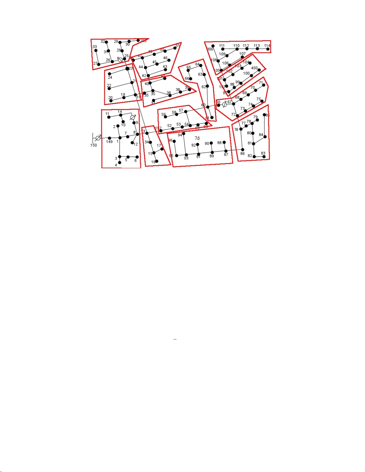
Generaliz ed gradient optimizati o n ov er lossy networks fo r partition-b ased estimation M. T odescato, N. Bof, G. Cavraro, R. Carli, L. Schenato October 31, 2017 Abstract W e address the problem of distributed con vex unconstrained optimization ov er networks characterized by asynchronous and possibly lossy communications. W e analyze t he case where the global cost function is the sum of locally coupled local strictly con ve x cost functions. As discussed in detail i n a motiv ating example, this class of optimization objecti ves is, for examp le, typical in loca lization problems and in partition-based state estimation. Inspired by a generalized gradient descen t strategy , namely t he block Jaco bi it eration, we propo se a novel solution which is amenable f or a distributed implementation and which , under a suitable condition on the step si ze, is prov ably locally resilient t o communication failures. The theoretical analysis relies on th e separation of time scales and L yapunov theory . In addition, to sho w the flexibility of the proposed algorithm, we deriv e a resilient gradient desce nt iteration and a resilient generalized gradient for quadratic p rogramming as two natural particularizations of our strategy . In this second case, global robustness is provided. Finally , t he proposed algorithm is numerically tested on the IE EE 123 nodes distribution feeder in the context of partition-based smart grid r obu st state estimati on in the presence of measurements outliers. 1 Introd uction The widesprea d of smart wireless elec tronic devices with the consequ ent creation of large-scale cyber-physical networked sys- tems pr omises a n ew rev olution in many field s. Howe ver , the se novel eng ineering systems and the ad vent of the “Big-Data” era requ ire the development of new compu ta tio nal paradigm s, d u e to the incr easing amo unt of devices and data to be consis- tently man a g ed. For example, many p roblems c a n b e cast as optimization prob lems. As so, in the last years the r e ha s b een a growing attention to d istributed op timization tools which have b ecome so impor tan t for two different reasons: first, the ad vent of Big Data asks fo r p arallelisation of the comp utational burden am ong m any pr ocessing un its since it is inconceivable to run o p timization algor ith ms o n one single (sup er)-comp uter . Sec o nd, many o p timization problems are sparse by nature since correlation between data is local. Nevertheless, one of the major hurdle to effecti vely deal with d istributed op timization u sing multiple proc e ssing un its is to guar antee synch ronou s a n d reliable commu nication. Ind eed, communica tio n can be wir eless and CPU execution times m ight not be kn own in advance as in the co ntext of clou d-comp uting. F or this reason , althoug h distributed o ptimization has a lo ng history in th e parallel and d istributed com putation liter ature, see, e.g. , [1], it has mainly focused on synchron ous algor ithms. However , to suitably fit with the upcom ing large-scale system scenario , in the last years it has been reconside r ed from a new peer-to-peer perspective. The first class of algorithm s appear in g in this new literature relies on pr imal sub-grad ient or d escent iterations, as in [2, 3, 4], which h av e the advantage to be ea sy to implemen t a n d suitable for asyn chrono us comp utation. In order to in duce robustness in the co mputation and improve con vergence speed, aug mented lagrangian algorith ms such as the Alternating Direction Method s of Multipliers (ADMM) have b een recently proposed . A first distributed ADMM algor ithm was propo sed in [5, 6 , 7], while a survey on this techniq ue is [ 8]. Howe ver, for a distributed implementatio n, ADMM usually r equires problem s with very specific structures. In fact, most of the ADMM d istributed algorithm s are b ased o n a con sensus iteratio n [9]. Thus, a comm on drawback of th is tech nique is that each node must stor e in its local me mory a co py o f the e n tire state vector . T o a void this problem, a recen t p artition-b a sed and scalab le appr o ach applied to the ADMM algor ithm is presen ted in [10], wh ile to comp ly with asyn chrono us comp utation, suitable m odification of the ADMM alg orithm have been prop osed in [1 1, 12]. Finally , distributed algorithm s based on Newton me th ods have been propo sed to speed-u p the com p utation [1 3, 14]. 1 M. T odescato, N. Bof, R. Carli and L. Schenat o are with the Departme nt of Information Engineeri ng, Univ ersity of Padov a, Italy , 35031. E-mail: [todesca t,bofnicol,ca rlirug,schenato]@dei.unipd.it. 2 G. Cavraro is with the V irginia Polytech nic Institut e ans State Univ ersity , V A, USA. E-mail: cavraro@vt.e du. 1 In this pap er , we ad dress the pr oblem of d istrib uted conv ex unco nstrained optimization over n etworks character ized by asyn - chrono us and possibly lossy co mmunicatio n s. W e analyze the case where the global co st f unction is the sum of loca lly cou pled local co sts. More spec ifically , by “lo cally coupled” and “d istributed” we mean the following Definition 1 (Local co upling and distributed algo rithm) Consid e r a set of N pr o cessing u nits, { 1 , . . . , N } , which ar e in - ter connected ac cor ding to a certain commu nication network. T o e a ch u nit i ∈ { 1 , . . . , N } a loc al cost J i is assigned . W e say tha t J i is lo cally coup led acco rding to the co mmunication network, if J i depend s only on quantities which are r elated to unit i and to un its dir ectly con nected to it. In this case, a distributed algorith m is a pr ocedu r e ru nning over the commun ica- tion network a n d amon g th e pr ocessing u nits, which on ly requir es the e xchange of lo c al info rmation amo ng con nected u nits. Differ ently said, with a slight abuse o f no m e n clatur e, a d istrib uted a lgorithm is defi ned as a locally co upled pr o cedur e.  Giv en Defin ition 1, this study is m o tiv a ted mainly by two facts. T he first is its practical en g ineering relevance. Indeed , as d iscu ssed in detail in a motiv ating example we p rovide in Section 3 , the structure o f the class of co nvex optimization problem s we analy ze, ch a racterizes a large variety of ap plications such as m ulti-area electric grid state estimation [1 5, 7], localization in mu lti-robo ts for mation [16] an d sensors networks [ 17] and Network Utility Maximization [ 18]. The second is d ue to the class of gradien t-based alg orithms (e.g., [2, 3, 4]) we co nsider to solve our op timization p roblem. In particular, while it has the advantage to be e a sy to im plement an d suitable for asynch ronou s implem e ntations, this class usually does not le a d to “distributed” solutio ns as inten ded in Definition 1. Ind eed, the derivati ves of costs obtained as the sum o f loca lly coupled costs are , usually , n ot locally coup led, yet th ey depe nd on info rmation related to multi-hop processing units. Hen ce, the lo cal func tional d ependan ce can not be dir e ctly exploited. T o overcome this issue, in so m e cases ([2, 3]) the algorithms require the lo cal exchange o f g lobal inform a tio n, hen ce all the proc e ssor s eventually reach consen sus to an optimal solution. In oth ers, the alg orithms requ ire mu ltiple comm unication r ounds within the same algor ithmic iter ation ([4]). Howev er, this solution imp licitly asks fo r synchr o nicity . Hen ce, to deal with th e case of lossy com munication s, a natu ral a p proach is to make the processing u nits store th e last successfu lly rec ei ved info rmation fro m the neighb oring un its in or der to leverage the vast existing b o dy of literature on the so called partially a syn chr ono us iterative method s [1]. However , as later describe d in Section 3, in this scen ario, because o f packet d rops and commu nication failures, the same state variables happen to app e ar in multiple delayed version. Th us, it is no t possible to write the ev olution o f the state variables as a partially asynchr on ous iterative metho ds . Finally , regarding the p roblem o f co mputing no n-locally coup led d eriv ati ves, anothe r used ap proach is to exploit hype r-comm unication g r aphs which differs f rom the grap h stru cture ind uced by the local coupling characteriz in g the cost fu nction, thus a r tificially bypa ssing th e limitations du e to a “truly” distributed p rocedur e. As a p articular example of th is fact, consider, for instan ce, the case wh ere the processors commun icate through a co mmunicatio n ne twork with star topo logy . According to Definitio n 1, eac h periph eral no de can commun icate only with the centr a l node, while the ce ntral pro cessor can commun icate with everyone else. Conv ersely , if a two-ho p commu nication is exploited , then the co mmunica tio n network turns ou t to be described by an all-to- all topology . In this regard, the main con tribution of the paper is a truly d istributed algo rithm, b ased on a mod ified gene ralized gradient descent itera tion which, under suitable assumption s on the step size, is pr ovably co nvergent a n d which is r e silient to th e presence of packet losses in the com m unication ch annel. T o the best of the au thors’ knowledge, this is one of the first provably conv ergent algorithm s in the p resence of packet losses, since even if bo th ADMM algorithm s and distributed sub- gradient method s (DSM) can hand le asynch ronou s comp utations, they still requir e reliable commun ication a n d usu a lly do not satisfy Definitio n 1. I nterestingly , the p roposed algorith m is also suitable f or fully parallel comp utation, i. e ., mu ltiple ag ents can commun icate and upda te th eir lo cal variable simultaneously , and for br oadcast commu nication, i.e., no d es do n ot need to en force a b idirectional commun ication such as in go ssip a lg orithms, an d theref o re is very attractiv e f rom a p ractical poin t of v iew . I t is anticipated that we presen ted the proposed alg o rithm in two p reliminary versions. In [19] for the specific case of qua d ratic pro grammin g , while in [1 7] for the specific application of sensors networks lo cations. The algor ithm is inspired on and resembles the block Jacob i iter ation a p peared in [1, 20]. Howev er , in [1], sin c e th e autho r s are majorly interested in parallel compu tation rather than implemen ting a distributed p rocedur e suitable fo r tod ay’ s sensors networks, th ey im p licitly assume to exploit an hy p er-communication graph. Conversely , in [2 0] th e particular local dependen cy considere d in the cost function en sures that first and suc c essi ve de riv ati ves are locally co upled. T o show th e flexibility of th e proposed pr ocedure , we deriv e a resilient gradie n t descent iteration and a resilient gen eralized gradient for q uadratic p rogramm ing as two natural particular izations o f our strategy . In this second case, we are able to provide global r o bustness. Finally , we nu merically study our a lgorithm on the standard I EEE 123 -nodes test feeder f or robust state estimation in the presence o f measure m ents outlier s. The rest of the pa per is organiz e d as follows: th e rest o f this section is devoted to th e necessary notatio n and prelimina ries. In Section 2 we for mulate the p roblem. In Section 3 we provide a motiv ating examp le fo r th e pr oposed set- u p. I n Section 4 we analyze the case of synchr onous an d id eal com munication s. In Section 5 we analyze the case o f asyn chrono us and possibly unreliable com munication s. In Section 6 we test o u r algor ithm. Fin ally , we p resent some con cluding remark s in Section 7. 2 1.1 Mathematical Preliminaries In th is p a p er , G ( V , E ) denotes a d ir ected grap h where V = { 1 , . . . , N } is the set of vertices and E ⊆ V × V is the set o f dir ected edges. Mo re precisely the edge ( i, j ) is incident on node i an d nod e j and is assumed to be directed away from i and directed tow ard j . The graph G is said to b e b idirected if ( i, j ) ∈ E imp lies ( j, i ) ∈ E . Given a d irected graph G ( V , E ) , a dir e cted path in G consists of a sequen ce o f vertices ( i 1 , i 2 , . . . , i r ) such that ( i j , i j + 1) ∈ E fo r every j ∈ { 1 , . . . , r − 1 } . The length of a path is th e number of dir ected ed ges wh ic h it consists of. The directed graph G is said to be str on gly connected if fo r any pair of vertices ( i, j ) th ere exists a dir ected path connec tin g i to j . G iven th e dir e c ted graph G , the set of neighb o rs o f nod e i , denoted by N i , is given by N i = { j ∈ V | ( i, j ) ∈ E } . Moreover, N + i = N i ∪ { i } . Let u s de note the car d inality o f N + i by µ i , while the j -th neighb or of i by N + i ( j ) . Given a dir ected graph G ( V , E ) with |E | = M , let the in cidence ma trix A ∈ R M × N of G be defined as A = [ a ei ] , whe r e a ei = 1 , − 1 , 0 , if edge e is in cident on node i a n d d irected away from it, is incident on node i and directed toward it, or is no t in cident on n ode i , respectively . Given a vector or a m atrix, with ( · ) ⊤ we denote its transpose, while with ℜ ( · ) and ℑ ( · ) its real a n d imagin ary parts, respectively . Given a vector v , with diag( v ) we denote the diagona l matrix wh ose diagona l elements are eq ual to the ele m ents of v . Given a matrix V , with diag ( V ) we den ote th e vecto r obtained with the d iagonal elemen ts of V . Gi ven a gr o up of m atrices V 1 , . . . , V n , with blkdiag ( V 1 , . . . , V n ) we deno te th e block diag onal m atrix whose i - th block diagon a l element is e qual to V i . Moreover , we de n ote with A d := A ⊤ A the a djacency matrix or laplacia n matrix of G which has the prop erty that [ A d ] ij 6 = 0 if and on ly if ( i, j ) ∈ E . If we associate to each edge a weight different fro m one, then it is possible to defin e the weighted lap lacian ma trix a s L = A ⊤ W A , wh ere W ∈ R M × M represents the diagonal matrix containin g in its i -th e le m ent the weight associated to the i -th edg e . W e will also con sider strictly co n vex fun ctions f ( x ) : R n → R , i. e., ∀ x 1 6 = x 2 and η ∈ (0 , 1) then f ( η x 1 + (1 − η ) x 2 ) < η f ( x 1 ) + (1 − η ) f ( x 2 ) and radially unb ounded , i.e. k x k → + ∞ ⇒ f ( x ) → ∞ . Finally , with the symb ols E and P we deno te, re sp ectiv ely , the expectation opera tor and the pr obability of an ev ent. 2 Pr oblem Formulation Consider a set o f N agents V = { 1 , . . . , N } , wher e each agent i ∈ V is describe d by its state vector x i ∈ R n i . Assum e the agents can co mmunicate among themselves throu g h a bidirected strongly conn ected communication graph G ( V , E ) . In this paper, we are interested in exten d ing to the mo re gen eral case of conve x costs the algor ithm first presented in [19] for the case of quadra tic progr amming an d in [1 7] for the specific applicatio n of sen sors network s localization. I n p articular, we examine a p articular class of separ a b le strictly con vex cost functio ns which exhib it local an d po ssibly non linear depe n dence among th e states o f ne ig hborin g nodes. By defin ing the overall state vector as x = [ x ⊤ 1 , . . . , x ⊤ N ] ⊤ ∈ R n ( n = P i n i ), we consider the following o ptimization problem min x J ( x ) ≡ min x 1 ,...,x N N X i =1 J i ( x i , { x j } j ∈N i ) . (1) Observe that th e lo cal d ependen ce coin cides with the comm unication g r aph G , i.e., each co st fu nction J i depend s o n in forma- tion regard in g on ly agent j ∈ N + i . W e will c o nsider the fo llowing assumptio n on the cost fucntion s: Assumption 2 (Strict c o n vexity and r adial unboundedness) The fun ction J ( x ) is assumed to be strictly conve x an d radi- ally u nboun ded.  Observe that un der the pr evious a ssumption the minimizer x ∗ of Prob lem (1) exists and is uniq u e x ∗ := a r gmin x J ( x ) , (2) but the local costs function J i do no t need to be strictly co n vex and r a dially unb ound e d . Indee d in many estimation prob lems the local cost functio ns J i are just strictly conv ex but not rad ia lly u nboun ded. The stan d ard appr o ach to so lve the previous optimization p roblem is to resor t to some c e ntralized iterativ e algo rithm acting on J , e.g., Newton-Raphson, which m akes use of g lo bal kn owledge of the network ’ states, costs an d topolo g y . On the contrar y , by leveraging the par ticular local depen dence characterizin g each cost f unction J i , we want to solve Problem (1) b y developing a procedu re wh ich is distributed , i.e. , exploiting o nly local exchan ge of inform ation amon g n eighbor s, a n d r esilient , i.e., resilient to co mmunica tio n limitations and non id ealities. W e will a lso use th e following simplified notation fo r local co mponen ts of g r adients and he ssians: ∇ i J j = ∂ J j ∂ x i , ∇ 2 iℓ J j = ∂ 2 J j ∂ x i ∂ x ℓ . 3 Remark 3 (On the class of separable cost functions) The class of functions co n sider ed can arise in diverse ap plications such as state estimation in smart electric grids [1 9] and senso r networks lo calization [17], ju st to mentio n some of them. In the particular case of qua d ratic co st, th e op timizatio n p r oblem falls onto the standa r d linear least-squa r es framework. Nevertheless, as it will be shown in the simula tion Sectio n 6, th e class is much mo r e general and co mprises pena lty fu nctions used, e.g., to perform r obust statistics and general non linear least-squ ar es optimization . Of particular inter est is the mor e general framework of parallel c o mputation in o ptimization. F or bo th priva c y and efficiency reasons, th e c omputatio n al bur den can be sp lit amon g several distributed machines. T o each of th e m only information ab o ut J i is assigned . Thank s to local exc hange of info rmation, the machine s must distributely c o mpute a solutio n of ( 1) .  Remark 4 (Partition-ba sed modular communication architecture) Note that the p articular c ommunicatio n a r chitectur e consid er ed, seamlessly d escribes the case of commun ications amo ng single pee r agents as well as among large areas co nsisting of a collection o f p e ers. The o nly differ ence r elies on the particular definition of the set V and of th e agents’ state x i . F or instance, in the case o f sensor localizatio n , each sensor migh t repr esent an agent of V while x i might describe its absolu te position in a n inertial global r efer ence frame. Conver sely , in the case of smart grids state estimation, one agent mig ht d e scribe an en tire electric feeder; then , x i would be either voltages or cu rr e n ts at a ll the electric buses of the co rr esp o nding feeder .  3 Motivating example: State es t imation in Smart Power Distribu tion Grids In steady state th e voltages and c u rrents in a p ower distribution gr id are regulated by the Kirchho ff ’ s laws which c a n be written as follow: Lv = i c , where L is the admittanc e matrix , a nd v an d i c are the vector collectin g all th e N voltages an d curren ts of the nodes in the g r id, respectively . The admittance matrix is a sp arse matrix, in the sense that the curren t at a specific node i , namely i c i , depen ds only o n its own voltage and the voltages o f its p hysically co nnected neig hbour n odes N i , i.e. i c i = X j ∈N + i L ij v j . In futu re smart distribution grid s, it is expe cted that each node i would b e able to take n o isy me a surements of its voltage and current, i.e. y v i = v i + w v i , y i c i = i c i + w i c i = X j ∈N + i L ij v j + w i c i , where w v i , w i c i represent the measuremen t n oise for the voltage and curren t measurements, respectively . It is also expected that these node s are embedd ed with commun ication c apabilities, such as p ower lin e co mmunica tion (PL C), wh ic h allow them to comm unicate with their phy sically conn ected neig hbour s. As so the comm u nication network and the physical n etwork will coincide. The (centralized ) state estimation p roblem is the proce ss that, given all the measurem ents { y v i , y i c i } N i =1 , shou ld return the b est estimate of all the voltages and cu rrents { v i , i c i } N i =1 . The standard ap proach is to cast this problem as a least-square estimation problem , wh ere the u nknown qu antities to be estimated a re th e voltages v ∗ , since th e cu r rents can be estimated directly from the voltages v ia the Kir chhoff ’ s law i c ∗ = Lv ∗ . In this work, we are in terested in solving this problem in a distributed fashion v ia a partition -based co mmunicatio n architecture. For th e sake o f clarity , let us assume that the g rid is divided into N partitions each corr espondin g to a nod e. T o ea ch p artition, we a ssoc ia te the cor respond ing voltage, which we collect in the vector x i ∈ R 1 . Let us also define with y i = [ y v i y i c i ] ⊤ ∈ R 2 and w i = [ w v i w i c i ] ⊤ ∈ R 2 the measur e m ent vector and the measu r ement noise co rrespon d ing to the measurem ents of the voltage and cur r ent at node i . Let us also de fine the vectors x = [ x 1 , . . . , x N ] ⊤ ∈ R N , y = [ y ⊤ 1 , . . . , y ⊤ N ] ⊤ ∈ R 2 N , w = [ w ⊤ 1 , . . . , w ⊤ N ] ⊤ ∈ R 2 N . As so the measur ement mo del can be written a s: y i = N X j =1 A ij x j + w i = X j ∈N + i A ij x j + w i ( A ij = 0 if j / ∈ N + i ) , where A ij can be e asily be ob tained from the elements of the matrix L , or equivalently in vector form y = Ax + w , 1 In reality , the voltages and currents in steady state are phasors, i.e., should be represented as complex numbers. Howe ver , the discussion in this section can be extended w .l.o.g. also to the more realistic scenario, which is indeed considered in the Simulation section below . 4 where A = [ A ⊤ 1 , . . . , A ⊤ N ] ⊤ ∈ R 2 N × N and A i = [ A i 1 , . . . , A iN ] ∈ R 2 × N . If we define J i ( x i , { x j } j ∈N i ) = 1 2 k y i − A i x k 2 , J ( x ) = N X i =1 J i ( x i , { x j } j ∈N i ) = 1 2 k y − Ax k 2 , with ∇ J ( x ) = A ⊤ ( Ax − y ) , ∇ 2 J ( x ) = H = A ⊤ A , H ij = N X ℓ =1 A ⊤ ℓi A ℓj = X ℓ ∈N + i A ⊤ ℓi A ℓj = X ℓ ∈ ( N + i ∩N + j ) A ⊤ ℓi A ℓj the o ptimal (centralized ) least squares solutio n 2 is given by : x ∗ = arg min x J ( x ) = ( A ⊤ A ) − 1 A ⊤ y . A stand ard approac h to asymptotically o btain the op tim al so lution is to employ an iterative algorith m based on the generalize d gradient descen t: x + = x − ǫD − 1 A ⊤ ( Ax − y ) = x − ǫD − 1 ∇ J ( x ) = x − ǫD − 1 ( H x − A ⊤ y ) , where ǫ is a su itab le stepsize and D is a strictly po siti ve definite matrix, i.e. D > 0 . A typical way to solve th e previous up d ate in a distributed fashion is to pick a bloc k -diagon al matrix D , i.e. D = blkdiag( D 1 , . . . , D N ) , so that the pr evious centr alized update c a n be written as x + i = x i − ǫD − 1 i ( N X j =1 H ij x j − N X j =1 A ⊤ j i y j ) = x i − ǫD − 1 i ( N X j =1 N X ℓ =1 A ⊤ ℓi A ℓj x j − N X j =1 A ⊤ j i y j ) = x i − ǫD − 1 i ( X j ∈N + ℓ , ∀ ℓ ∈N + i A ⊤ ℓi A ℓj x j − X j ∈N + i A ⊤ j i y j ) , (3) where we exploited th e p roperty tha t A ij = 0 if j / ∈ N + i . While the second summation in volves only measu rements that belongs to the neig hbour s o f no de i , th e first summatio n requir e s the nod e i to co llect the state variables x j that belong s to the neig hbour s of the neigh b ours. As so, this imp lementation is not really distributed, since two-hop commun ic a tion is required . Althoug h this is no t imp ossible from a practical perspective, it requ ir es substantial add itional c ommun ica tion and synchro n ization e fforts. An alter nativ e appro ach which allows the implem entation of a truly d istributed algor ithm is to cr eate the ad ditional local variable at each node i : z i = A i x i = X j ∈N + i A ij x j , ∀ i , which can be co llected in the vector z = [ z ⊤ 1 , . . . , z ⊤ N ] ⊤ , so that in matrix form the p revious expression can be written as z = Ax . W ith this notation the generalized grad ient descent can be written as: z + i = X j ∈N + i A ij x j x + i = x i − ǫD − 1 i ( N X ℓ =1 A ⊤ ℓi N X j =1 A ℓj x j | {z } z ℓ − N X j =1 A ⊤ j i y j ) = x i − ǫD − 1 i X j ∈N + i A ⊤ j i ( z + i − y i ) . 2 The formulation can be extended to the weighed least square solutions if noise with diffe rent varian ces R are included which would lead to the s olutio n x ∗ = ( A ⊤ R − 1 A ) − 1 A ⊤ R − 1 y , but for the sake of clarity in the notation of this section, it is om itted. 5 This alterna ti ve solution req u ires two commu nication round s to comp ute x + i , since first it is necessary to send the x i to compute z + i , and then to transmit z i to the neighb ours 3 . In pr actical scena r ios, such as using PLC pro tocols, synchro nization of tr ansmissions an d u pdates ca n be difficult. Mor eover packet losses mig ht occ ur , i.e. some messages fr om the neigh bours might not be received. A naive solution to this prob lem, is to use local registers that keep in memory the latest message received from the neigh bours, and then use the se values when ever an update of the lo cal variables x i , z i is neede d . It ca n be shown that this is equiv alent to a scenario where ev ery n ode j ∈ N i use a d elayed version of the local variables x i , z i . Since the variables z i are function of the (possibly delayed ) state variables x i , the variables x i are themselves f u nctions of the delayed version of variables x i of the network. M o re specifically , it c a n be shown that the p revious upd ate equation s c an be written as z i ( t + 1) = X j ∈N + i A ij x j ( τ ′ ij ( t )) , (4) x i ( t + 1) = x i ( t ) − ǫD − 1 i  N X ℓ =1 A ⊤ ℓi N X j =1 A ℓj x j ( τ ℓj ( t )) − N X j =1 A ⊤ j i y j  . (5) where 0 ≤ τ ij ( t ) , τ ′ ij ( t ) ≤ k repr esent the delay of each variable which d epends on the specific sequen c e of packet losses and variable up dates, and explicitly in cluded the tim e dep endency of each variable. No te that in th e last equation the variable x j might ap pear with multiple instance s with different delay s into the upd a te of the variable x i , i.e. it is n ot p o ssible to write the evolution o f variables o f the origina l ge n eralized gradient descen t algorithm given in Eq n. (3) as a partially asynchr o nous iterative methods ( see chapter 7 of [ 1]), for wh ich en extensive body of liter ature exists, since the cited fr amew ork would require the algor ithm to be wr itten as: x i ( t + 1) = x i ( t ) − ǫD − 1 i  N X j =1 H ij x j ( τ ij ( t )) − N X j =1 A ⊤ j i y j  . (6) Motiv ated by this observation, in this work we will p ropose an altern ativ e math ematical machine ry based on L yapunov theory and the sepa r ation of time scale principle to p rove convergence o f the asy n chron o us algor ithm (5) f or a sufficiently small stepsize ǫ . Note that this mac h inery can also be app lied to mo re g e neral convex problem s. This is useful, for example , in the presence o f outliers or sensor faults in order to d ev elop m ore ro bust estimators tha n least squ ares. In fact, a comm on way to enforce robustness in the e stima tio n is to rep lace the quadratic cost function d efined above with th e 1-nor m o f the residuals, that is J i ( x i , { x j } j ∈N i ) = k y i − A i x k 1 . (7) Howe ver , since (7) is not differentiable, it cannot be directly u sed with our algo rithm. T o deal with th is issue, in the Simu lation section 6, we will exploit the following modificatio n of the 1-n orm [21] k · k 1 ,ν : R n → R , x 7→ k x k 1 ,ν := N X i =1 q x 2 i + ν , (8) where ν > 0 is suc h th at th e smaller the selected value o f ν is, the better the ap proxima tion o f th e 1 -norm is. In particu lar , the approx imation of each term in the summa tio n of the cost f u nction is quad ratic when x i belongs to a small neighb orhoo d o f 0 . The n ext Sections will then provide a fully distributed g eneralized grad ie n t descent alg orithm which is resilient to lossy commun ication. 4 Synchr onous update and rel iable com m unication In th is section we analyze the case of syn chrono us and id eal, i.e., reliable, co mmunica tio ns amon g n eighbor s, leaving the extension to th e more realistic case of u nreliable comm unication to Section 5 . Consider the op timization Problem (1). In the id eal com munication case, on e possible ch oice to iteratively solve Problem (1) is to exploit the so called generalized gradient descent iteration x + = x − ǫD − 1 ( x ) ∇ J ( x ) , x (0) = x 0 , (9) 3 It is necessary to transmit the measurements y i only at the initial izatio n phase since they do not change during the course of the evol ution of the algorithm. 6 where ∇ J ( x ) := h ∂ J ( x ) ∂ x | x i ⊤ is th e gr adient of J ev aluated at the cur r ent value x , D ( x ) is a g eneric po siti ve definite matrix, possibly function of x itself, and ǫ a suitable positive co nstant, r eferred to a s step size . Ob serve that depend ing on th e par ticu lar choice o f D ( x ) , Eq. (9) describes various types of algor ithms. Ind eed, if D ( x ) = I , the standard gr adient descen t iteration is obtained; if D ( x ) is cho sen to be diagon a l with diagona l elem e nts equal to those of the Hessian matrix, then a Jacobi descen t iteration is retrieved; wh ile, if D ( x ) is eq ual to the en tire Hessian, then Eq. (9) return s th e classical Newton-Raphson iteration . The algorithm we prop ose (and describe in Section 5) is inspire d by the pa rticular case o f ( 9), refer red to as block Jacobi , where we choo se D ( t ) to be the b lock diago nal ma trix such th at D ( x ) = blk dia g( D 1 ( x ) , . . . , D N ( x )) , D i ( x ) := ∇ 2 ii J ( x ) , i ∈ V , (10) i.e., where each diagon al block coincides with the second orde r derivati ve of J w . r .t. x i . Th a nks to this choice for the matrix D , Eq . (9) can be split into par tial state up dates e a c h of wh ich equa l to x + i = x i − ǫD − 1 i ( x ) ∇ i J ( x ) , i ∈ V . (11) Now , it is con venient to explicitly take into a ccount the separab le structure of the cost f unction J in ord e r to show that each gradient block ∇ i J as well as ea ch D i block can be com p uted exploiting only local inf ormation comin g fro m age n t’ s i two-steps n e ighbors , i.e., agents con n ected to agen t i by a directed path of len gth two. In deed, for the gradient we h av e that ∇ i J ( x ) = X j ∈N + i ∇ i J j ( { x k } k ∈N + j ) = ∇ i J i ( x i , { x j } j ∈N i ) + X j ∈N i ∇ i J j ( x j , { x k } k ∈N j ) , (12) and it can be seen that the first term on the RHS of Eq. ( 1 2) depends o n ly on inform ation coming from j ∈ N + i ; while, the second term depend s o n infor mation co ming from neighbor s of n ode i a nd fro m the neigh b ors o f its neig hbors, k ∈ N + j . A similar re asoning applies to D i indeed, D i ( x ) := X j ∈N + i ∇ 2 ii J j ( { x k } k ∈N + j ) = ∇ 2 ii J i ( x i , { x j } j ∈N i ) + X j ∈N i ∇ 2 ii J j ( x j , { x k } k ∈N j ) . (13) Again, the first term in the RHS of Eq. ( 13) depen ds only on nod e i d irect neighbo rs, j ∈ N + i , while the secon d term req uires informa tio n comin g f r om the neigh bors of its neighb ors. I n view of a distributed com putation, we assume each agent i ∈ V , once gathered the neighb ors states { x j } j ∈N i , c a n com pute and store in its local m emory , in additio n to the state x i , th e following variables ρ ( j ) i ( x ) := ∇ j J i ( x i , { x j } j ∈N i ) , ξ ( j ) i ( x ) := ∇ 2 j j J i ( x i , { x j } j ∈N i ) , (14) which rep resent the p artial compo nents of the first an d seco nd deriv atives of its local cost J i ev aluated at the curre nt state value. Ob ser ve that, since in a distributed framework eac h ag ent is assumed to h av e in formatio n only regarding its local c o st J i , th e ρ ’ s and ξ ’ s variables rep resents the q uantities which agent i mu st compu te a nd send to its neigh bors in orde r to let them compute their cor respondin g gr a dient and hessian b lo cks. Likewise, agent i needs to rece ive similar variables from ea c h one of its neigh bors. In deed, thank s to Eqs. ( 12)–(13), it ho lds that ∇ i J ( x ) = X j ∈N + i ρ ( i ) j ( x ) , D i ( x ) = X j ∈N + i ξ ( i ) j ( x ) . (15) As above stressed, each agent i ∈ V , to iter ati vely co m pute (11), can perfo rm its compu tations auto nomou sly assuming it h as at its disposal info rmation coming fr om its two-steps neigh bors. Howe ver , this p resents two major drawbacks: 1. it clashes with a tru ly distributed setting which exploits the exchan g e of inform a tion only among on e-step neighbo rs; 2. within successiv e iterations, to ensure con sistency and thu s co n vergence of the proc edure to a minimizer o f Problem (1), all the commun ications mu st be synch ronou s an d reliable. T o workaro und the fir st issue one possible solu tion would be, at each iteratio n, to p e rform two comm unication r o unds amon g one-step neighbo rs as illustrativ ely sh own in Figu re 1. Th e first r ound is u sed to exchange th e state values am ong neig h boring agents in o rder them to com pute all th e partial infor mation term s acco rding to Eqs. (1 4)–(15); wh ile the second ro und is 7 Agent i : 1st comm. round compute n ρ ( j ) i ( t ) , ξ ( j ) i ( t ) o j ∈ N + i to j ∈ N i from j ∈ N i x i x j 2nd comm. round update x i ( t ) single iteration to j ∈ N i from j ∈ N i { ρ ( j ) i , ξ ( j ) i } { ρ ( i ) j , ξ ( i ) j } Figure 1: Communicati on scheme to perform one single block Jacobi itera tion (11) in a distribute d settin g which assumes only information exch ange among one-step neighbors. used to co mmunicate the comp uted variables in ord er to perfo r m the state u pdate as in Eq . (11). Re garding the secon d issue, it necessarily enf orces the use of suitab le syn chroniza tion algorithm s as well as re-transmission pro tocols in case o f packet failures. What above d escribed has been compac tly written in algorith mic form as repo rted in Algor ithm 1 in wh ich flag transmission denotes a variable to c ontrol c o mmunica tio n an d upd ate amon g the ag ents. Note th a t, ev en if these might provide possible answers, it is under sto o d th ey do no t re p resent satisfactory solutions for real-world applications. Conversely , in the next sectio n we pro pose a truly distributed and resilient iter ativ e proc e dure wh ic h , by natur a lly exploitin g in f ormation coming fro m one-step neigh bors an d being resilient to packet losses an d commu nication non idea lities, is much more a ppealing from an engin eering per spectiv e. Algorithm 1 Distributed Block Jacobi a lg orithm (no de i ) . Require: x o i , ǫ 1: x i ← x o i 2: if fla g transmission = 1 then 3: Broadcast : x i 4: Receive : x j , ∀ j ∈ N i 5: ρ ( j ) i ← ∇ j J i ( { x k } k ∈N + j ) , ∀ j ∈ N + i 6: ξ ( j ) i ← ∇ 2 j j J i ( { x k } k ∈N + j ) , ∀ j ∈ N + i 7: Broadcast : ρ ( j ) i , ξ ( j ) i , ∀ j ∈ N i 8: Receive : { ρ ( i ) j , ξ ( i ) j } , ∀ j ∈ N j 9: x i ← x i − ǫ  P j ∈N + i ξ ( i ) j  − 1  P j ∈N + i ρ ( i ) j  10: end if 5 Asynchr onous updates and unre liable comm unication: the Resilient Block Ja- cobi (RBJ) algorithm In this section we conside r the m ore realistic case of asynchro nous and un r eliable comm unications wh ere eac h agent might either receive asynch ronou s in formation coming fr om its neigh b ors, or not r eceiv e it. I n particular, we present a mo dified iteration an d analyze its correspo nding iterative algo rithm, which we re f er to as r esilient block J acobi , which (i) exploits only informa tio n coming from one-step n eighbo r s; (ii) r e quires on ly one com m unication roun d per algorithm ic iteration; (iii) is based o n an asynchr onous co mmunicatio n proto c ol; (iv) is resilien t to commu nication failures. First, w e present ou r algorithm for the gen eral case of separab le conve x costs. Later , we particular ize th e algorithm to suit two special ca ses an d showing its flexibility . Consider th e standard blo ck Jacobi iteratio n (11). As analyze d in Section 4 , th e proced ure exhibits some fu ndamenta l crit- icisms which deeply compro mise its distributed an d asynchron ous im plementation an d yet its ro bustness p roperties. Th us, to develop our algorithm , we nee d to suitably modify iteration (11). Th e modification we propo se is app arently na ive since the idea is to simply equip each agent with an additional amount of memory stor age to keep track of the last received and av ailable inf ormation cor respond ing to each neig hbor . This ad ditional memo r y is then used to perfo rm Eq. (11). Indeed note that, if a gent i does no t receive some of the inf ormation comin g fro m its neighb o rs, it does n ot have the necessary infor mation to syn chrono usly compu te neither (14) n o r (15) and thus it is not able to u pdate its state acco rding to (11). 8 x i ( t ) , n ρ ( j ) i ( t ) , ξ ( j ) i ( t ) o j ∈ N i n b x ( i ) j ( t ) , b ρ ( i ) j ( t ) , b ξ ( i ) j ( t ) o j ∈ N i Agent i Agent j ∈ N i x i ( t ) , ρ ( j ) i ( t ) , ξ ( j ) i ( t ) γ ( j ) i x j ( t ) , ρ ( i ) j ( t ) , ξ ( i ) j ( t ) γ ( i ) j Figure 2: Memory storage and communication scheme between pairs of neighbors agents for the RBJ algorithm. T o mod el ra n domly occurr ing pa cket losses is co n venient to introdu ce the in dicator fun ction γ ( i ) j ( t ) =  1 if i received th e infor mation sen t by j at iter ation t 0 otherwise. with the assumption that γ ( i ) i ( t ) = 1 , since node i has always access to its lo cal variables. The n , as suggested above, th e main idea is to equ ip each agent i with au xiliary variables n b x ( i ) j , b ρ ( i ) j , b ξ ( i ) j o j ∈N i , u sed to keep tr ack of the last available info rmation received from each neigh b ors. Specifically , the dy namic for th e j -th set of ad ditional variables is given by n b x ( i ) j ( t ) , b ρ ( i ) j ( t ) , b ξ ( i ) j ( t ) o =        n x j ( t ) , ρ ( i ) j ( t ) , ξ ( i ) j ( t ) o , if γ ( i ) j ( t ) = 1 ; n b x ( i ) j ( t − 1 ) , b ρ ( i ) j ( t − 1 ) , b ξ ( i ) j ( t − 1 ) o , if γ ( i ) j ( t ) = 0 . (16) Thanks to this addition al mem o ry at every algo rithmic iteratio n, each agent can per form its lo cal update which, inspired on Eq. (1 1), becomes equ al to x i ( t + 1) = x i ( t ) − ǫ   X j ∈N + i b ξ ( i ) j ( t )   − 1   X j ∈N + i b ρ ( i ) j ( t )   . (17) Observe that the differences between Eqs. (1 1) and (1 7) are main ly two: 1. the variables in agent i ’ s m emory , used to stor e the first an d second pa r tial d eriv ati ves of J i w .r .t. j ∈ N i , are necessarily computed as ρ ( j ) i ( t ) = ∇ j J i ( x i ( t ) , { b x ( i ) k ( t ) } k ∈N i ) , ξ ( j ) i ( t ) = ∇ 2 j j J i ( x i ( t ) , { b x ( i ) k ( t ) } k ∈N i ) , (18) that is, they are ev aluated at the last stored states’ values; likewise, the values o f the addition al variables { b ρ ( i ) j , b ξ ( i ) j } j ∈N i correspo n d to those last received from each neig hbor a n d com puted by each of th em using the last av ailable info rmation on their neighb ors’ states; 2. con versely to the synchr onous impleme n tation of th e algorithm, at ea c h iteration only on e com munication roun d is perfor med. Th is m eans the ag e n ts send only one packet p e r iteratio n, con sisting of the state and the partial deriv ativ es. See Figu re 2 for an illustrative re p resentation. Thanks to this simple modification the agents can p erform their updates asynch r onously and in d ependen tly . Moreover, since only o ne comm unication ro und per iteration is re q uired, both th e commu nication burden and the nu m ber of po ssible commu - nication failures are reduced . Nevertheless, it is worth stressing th at, even if no packet losses occu r, the classical block Jacobi and ou r resilient b lock Jacobi iteration do es not exactly coincide. Indeed , in th e resilient case, b y sending only one packet p e r iteration, the state and the p artial derivati ve informatio n would be “d elayed” one from each other of on e iteration if co m pared with the synchr onous implem e ntation. The res ilient block Jacobi a lg orithm (her e after r eferred to as RBJ algorithm) for sep- arable con vex fun ctions is formally described in Algorith m 2 wh e r e it is presented in an ev ent-based up date perf ormed by a generic n ode i . The variables fla g transmission , fl ag reception , fl ag update are flag variables which d e termines which specific action a node is p e rformin g, name ly transmission, r eception or u pdate. Wh e n each action is perfor med it can not be inter- rupted, howe ver the specific ord er o r consecu ti ve calls of an action d o not im p air th e conv ergence of the propo sed algorith m and ther efore can be used in depend e n tly of the specific comm unication p rotocol or CPU multitaskin g sch eduling. 9 Algorithm 2 Resilient Block Jacobi (RBJ) Algorithm (n ode i ) Require: x o i , ǫ Initialization (atomic) 1: x i ← x o i 2: b x ( i ) j ← 0 , ∀ j ∈ N i 3: ρ ( j ) i ← 0 , ∀ j ∈ N i 4: b ρ ( i ) j ← 0 , ∀ j ∈ N i 5: ξ ( j ) i ← I , ∀ j ∈ N i 6: b ξ ( i ) j ← I , ∀ j ∈ N i 7: flag transmission ← 1 ( optional) T ra nsmission (atomic) 8: if fla g transmission = 1 then 9: transm itter node ID ← i 10: ρ ( j ) i ← ∇ j J i ( x i , { b x ( i ) k } k ∈N i ) , ∀ j ∈ N i 11: ξ ( j ) i ← ∇ 2 j j J i ( x i , { b x ( i ) k } k ∈N i ) , ∀ j ∈ N i 12: Broadcast : transmi tter node ID , x i , { ρ ( j ) i , ξ ( j ) i } j ∈N i 13: flag transmission ← 0 14: flag reception ← 1 ( optional) 15: end if Reception (atomic) 16: if flag reception = 1 then 17: j ← t ransmi tter node ID 18: b x ( i ) j ← x j 19: b ρ ( i ) j ← ρ ( i ) j 20: b ξ ( i ) j ← ξ ( i ) j 21: flag reception ← 0 22: flag update ← 1 (op tio nal) 23: end if Estimate update (ato mic) 24: if flag update = 1 then 25: b ρ ( i ) i ← ∇ i J i ( x i , { b x ( i ) k } k ∈N i ) 26: b ξ ( i ) i ← ∇ 2 ii J i ( x i , { b x ( i ) k } k ∈N i ) 27: x i ← x i − ǫ  P j ∈N + i b ξ ( i ) j  − 1  P j ∈N + i b ρ ( i ) j  28: flag update ← 0 29: flag transmission ← 1 ( optional) 30: end if 10 Remark 5 (Resilient gra dient descent ( R G D) Algorithm) If memory , co mmunication and computation al complexity ar e a concern, it is possible to modify the pr oposed algorithm mimicking the standard gradient descent a lgorithm. In this framework, the seco nd order in formation is not neede d a nd therefor e the variables ξ ( i ) j , b ξ ( i ) j ( lines 5, 6, 17, 21 in Algorithm 2) do no t need to be compu ted a nd the upd ate for the local variable x i ( line 22 in Alg o rithm 2) sho u ld b e replaced with the following: x i ← x i − ǫ X j ∈N + i b ρ ( i ) j . Obviously , the price to pa y for this choice is a likely decr ease in co n ver gence speed . Remark 6 (Resilient W eig hted Least Squares (RWLS) Algo rithm) If the lo c a l cost functio ns ar e qua dratic, i.e: J i ( x i , { x j } j ∈N i ) = 1 2 k y i − A i x k 2 W i = 1 2 ( y i − X j ∈N + i A ij x j ) ⊤ W i ( y i − X j ∈N + i A ij x j ) , wher e W i > 0 are the lo c a l weigh ts, th en th e pr o blem to be solved becomes a W eigh ted Least Squ ar es pr oblem. F or this special case, the gradient and the hessian co mponents simplify to: ρ ( j ) i ( x ) := A ⊤ ij W i ( X j ∈N + i A ij x j − y i ) , ξ ( j ) i ( x ) := A ⊤ ij W i A ij , (19) ther efor e the RBJ Alg o rithm c an be simplified by substituting lines 10 a nd 11 with the fo llowing upda tes: ρ ( j ) i ← A ⊤ ij W i ( A ii x i + X j ∈N i A ij b x ( i ) j − y i ) , ∀ j ∈ N i , (20) ξ ( j ) i ← A ⊤ ij W i A ij . (21) It is clear fr om the pr evious expr ession, that the a lgorithm cou ld be modifi e d by havin g a preliminary pha se when the ξ ( j ) i ar e transmitted r eliably to the n eighbou rs so that eventually b ξ ( j ) i = ξ ( j ) i , and then the algorithm co uld simply transmit the variables x i , ρ ( j ) i and u pdate th e variab les x i , b x ( i ) j , b ρ ( i ) j which are the only variables that evolve over time, thus c onsiderably r educing the co mmunicatio n comp lexity which corr espond s with that o f the RGD algo rithm . 5.1 Theor etical analys i s of RBJ Algorithm Before presentin g the major theor etical result characterizin g the co n vergence pro perties o f the prop osed RBJ algorithm, we introdu c e th e fo llowing assumptio n o n the natur e of lossy comm unication we co nsider . It m ainly states th at each agent i ∈ V receives infor mation coming from ea ch agent j ∈ N i at least once within a ny wind ow of T iterations of the a lg orithm. Assumption 7 (Persistent communication) Ther e exists a constan t T such that, for all t ≥ 0 , for all i ∈ V and for all j ∈ N i , P h { γ ( i ) j ( t ) , . . . , γ ( i ) j ( t + T ) } = { 0 , . . . , 0 } i = 0 .  Theorem 8 (Lo c al c o n vergence of the RBJ algorithm) Let Assumptions 2 a nd 7 hold. Moreover assume that the co st func- tions J i ar e thr ee-time differ en tiable and contin uous. Consider Pr oblem (1) an d th e RBJ algo rithm. Let x ∗ be the minimizer of (1) . There exists ¯ ǫ > 0 an d δ > 0 , such that, if 0 < ǫ < ¯ ǫ and k x (0) − x ∗ k < δ , then th e trajectory x ( t ) , generated by the RBJ a lgorithm, conver ges exponentially fast to x ∗ , i.e., k x ( t ) − x ∗ k ≤ C ρ t for some constants C > 0 and 0 < ρ < 1 .  The pro of of The o rem 8 c an be fo und in App endix A, and b asically relies on separa tion o f time scales princip le between the dynamics of the states x i ’ s and those of th e auxiliary variables b x ( i ) j ’ s, ρ ( i ) j ’ s, b ρ ( j ) i ’ s, ξ ( i ) j ’ s and b ξ ( j ) i ’ s. L o osely speaking , the result builds on the idea th at if th e step- size ǫ is small enou gh, the variation o f the true states x i ’ s is sufficiently slow and , despite the lossy co m munication , the values of the auxiliary variables stored in memo ry eq ual the tru e values. 11 Remark 9 (Local co n vergence of the RGD a lg orithm) Th e same a r gument used in the pre vious theor em can be app lied to the R o bust Gradient Descent Algorithm p r esented in Remark 5 ab ove under th e weaker assumption th at the cost function s J i ar e two-time differ en tiable, thus pr ovidin g the same local exponential conver genc e. T ypica lly , th e critica l value ¯ ǫ for th e R GD algorithm is smaller th an that of the R B J algorithm, an d consequen tly also th e rate of co n ver gence is slower .  Lemma 10 (Global conver gence R WLS a lgorithm) Let Assump tions 2 and 7 h old. Consider Pr o b lem (1) with a qua dratic cost function J ( x ) and th e RWLS algorithm. Ther e exists ¯ ǫ such that, if 0 < ǫ < ¯ ǫ , then, for any x (0) ∈ R n , the trajectory x ( t ) , generated by th e RWLS algorithm, conver ges exponentially fast to th e minimizer x ∗ of the co rr esp o nding pr oblem, i.e., k x ( t ) − x ∗ k ≤ C ρ t for some constants C > 0 and 0 < ρ < 1 .  6 Simulations In this section we pr esent som e simulative r esults o btained u sing th e RBJ algorith m. The simulations in volve the IEEE 123 nodes distribution g r id bench mark ( see [7]). The pr oblem we ad dress is the robust estimation of the voltage level at each node of th e gr id (excep t the PCC node wh ich is assumed fixed and known) f rom voltage and cu rrent me a surements in the presence o f measure m ents outlier s. W e recall that voltages an d curr ents in an A C power distribution g rid are com p lex values. Howe ver , in view o f th e state estimation pro blem we con sider , it is conv enient to exploit an equ ivalent standard reformu lation in rectan gular coo rdinates. In par ticular , given the complex vectors of voltages and currents, den oted as v ∈ C 122 and i c ∈ C 122 respectively , and th e weig hted Laplac ian matrix L ∈ C 122 × 122 describing the electric gr id, th anks to Kirchh o ff ’ s voltage and cur rent laws, it hold s tha t i c = L v . (22) Howe ver , by r ewriting voltage and cur rents in rec ta n gular coordin ates as v := [ ℜ ( v ) ⊤ ℑ ( v ) ⊤ ] ⊤ ∈ R 244 , i c := [ ℜ ( i c ) ⊤ ℑ ( i c ) ⊤ ] ⊤ ∈ R 244 . and, similarly , by splitting L into its real a nd imagin ary p arts as L =  ℜ ( L ) −ℑ ( L ) ℑ ( L ) ℜ ( L )  , Eq. (2 2) is equivalent to i c = Lv . Thus, by assuming to collect bo th current and voltage measure m ents directly in rec ta n gular coordin ates 4 , our measur ement model r e ads as  y v y i c  =  I L  v +  w v w i c  +  o v o i c  ,  w v w i c  ∼ N  0 0  ,  σ 2 v diag( | v | ) σ 2 i c diag( | i c | )  , where I ∈ R 244 is th e identity m atrix, y v , y i c ∈ R 244 are the measurem ents, which we co llect in vecto r y ∈ R 488 , w v , w i c ∈ R 244 are the measuremen ts’ no ise, and o v , o i c ∈ R 244 are sparse vectors which c ontain possible measur ement ou tliers. W e choose 5 σ v = 1 0 − 3 [p.u.] and σ i c = 1 0 − 1 [p.u.] . Finally , conc e r ning the outliers, 1 0% of the measu rements are corru pted, and the distribution of the outliers is uniform between 1 / 10 0 and 1 / 80 of the respective me a surement fo r voltages and between 1 / 2 an d 1 o f the respe cti ve c urrent measur e ment. As suggested at th e end of Section 3, to perf orm robust state estimation in the p resence either of measurem e nts faults or outliers, on e interesting cho ice for the c ost fu n ction is the mo dified 1-no r m defined is Eq . (8) as k r k 1 ,ν where r = y − Av are the m easurements r esiduals with A = [ I L ⊤ ] ⊤ . T o ru n th e RBJ algo rithm we need to ide ntify some partition of the grid. T o d o so, the feed er is d i vided into N n on overlapping areas, and a co mputing unit, which can collect 4 Accordin g to future smart grids paradigm, it is assumed each node of the grid to be equipped with a smart m easuremen t units, e.g., a P hasor Measurement Unit (PMU), which can return m easurement s of current and voltage . Usually , electric quantities are measured in polar coordinat es. Howe ver , for the s ake of simplicit y , we assume to hav e at our disposal measurements direct ly in recta ngular coordina tes, stressing that, thanks to a suitable lineariza tion, it is al ways possible to pass from polar to rectangula r coordinat es. 5 The choice for the m easurement s error standard de viations is dictated by the fact that the de facto standard for m odern PMUs require s at most a 0 . 1% error in the volta ge m easuremen ts. This translate s in a current error of more or less 10% . 12 PCC Figure 3: Di vision in N = 13 areas of the IE EE 123 nodes distributio n grid. the m easurements of the nod es be lo nging to the area an d can run the algo rithm, is associated to each area. An example of th e division in ar e as is given in Figu re 3. Th e commun ication gra p h G can be obtain ed fr om the division in areas, an d in particular, two u n its ca n commun icate with each other if the two ar eas are ph ysically conn ected (that is if there exists two nodes, each one belong ing to one of the areas, which are co nnected by an electric wir e). Th e vector s y , x an d r a n d matrix A are di vided accordin g to the par tition of the n odes in a r eas. Given the cost fun ction, th e values o f ρ ( i ) j and ξ ( i ) j are comp uted as: ρ ( i ) j = A ⊤ j i  (diag( r j ( t ))) 2 + ν I  − 1 / 2 r j ( t ) , ∀ j ∈ N + i ξ ( i ) j = ν H ⊤ j i  (diag( r j ( t ))) 2 + ν I  − 3 / 2 H j i , ∀ j ∈ N + i . W e tested the RBJ algo rithm unde r two d ifferent scen arios to ev aluate the influence o f different param e te r s inv olved in the algorithm . All the re sults showed a re obtaine d a veraging over 1 00 Monte Carlo runs (MCR). In the first considere d scenario we study the in fluence of the n umber N o f areas on th e perfor mance of th e algorithm . Observe tha t, fo r the case N = 1 the propo sed RBJ algorithm resembles a Newton-Raphson iteration. Thus, in general and as shown in Figure 4, the fewer the num b er of areas, the faster the conver gence rate. In the second scenario we analyze the influence of th e step size ǫ on th e conv ergence rate . As can be seen from Figure 5, we can infer that the conver gence rate improves for bigg er values of ǫ . Nevertheless, it is importan t to high light the fact that that the algor ithm m ay diver ge if the selected ǫ is a to o large. Finally , we have considered a th ird scenario, not rep orted r e ported here, in wh ich the robustness of the algorith m is tested for incr easing values of the packet loss prob ability . The re sults show that th e algo rithm is really robust to packet losses as can be seen both fro m Figures 4 – 5 whe r e the algorith m h a s been tested con sidering a 30% packet loss p robability . In particu lar , since the cu rves o btained are re a lly close to each o ther, we decide d n o t to show the results of the simu lations. A s last re m ark regard ing the pa c ket loss scenario, it is nu merically observed that the h igher th e pa c ket loss pro bability , the sm aller the value o f the step size to ensure convergence of the algo r ithm. Therefo r e, in the c h oice of the step size of the algor ithm, which is still an open problem, the degree of r eliability of the co mmunica tio n network must b e considered . 7 Conclusions Considering the emerging area of large-scale multi- a g ent systems, this paper addressed the always m o re timely pro blem of unconstra ined robust distributed conve x optimization in the presence o f co mmunicatio n n o n idealities. In particular, we analyzed a particular c lass of locally cou pled cost function s wh ich ar ise in d i verse interesting engin eering prob lems such as multi-area state estimation of smart electric grids an d m ulti-robo t loc alization, just to men tio n two possible application s. W e considered a particularly flexible partition -based commun ication architectu re which seamlessly accou n ts for peer-to-peer and 13 Figure 4: Normalize d cost function as a function of the iterati on, for diff erent numbers of areas N . In all simulations there is a pack et loss probability of 30% and ǫ = 0 . 0004 . The results are obtaine d ave raging ove r 100 MCR. Figure 5: Normalize d cost function as a function of the iteration , for dif ferent values of the parameter ǫ . The number of areas used is N = 13 and the results are obtained ave raging over 100 MCR. In all simulations there is a packet loss probabilit y of 30% . 14 wide-area commu nications. W e prop osed a gene ralized g radient alg orithm b a sed on the well-known Jacobi iteratio n. By lev eraging L yapu nov theory an d separation of time scale p rinciple, we p roved r obustness of the algorithm to packet drops and commun ication failures. Finally , we extensively tested the p roposed solution for robust state e stima tio n in the presen ce of measuremen ts ou tliers using as bench mark the standard IEEE 123 no des distribution feeder . A Proof of Theorem 8 The proof of Theor em 8 relies on th e time scale sep a r ation of th e dy namic of th e x i ’ s a nd of the auxiliary variables b x ( i ) j ’ s, b ρ ( i ) j ’ s an d b ξ ( i ) j ’ s, and fu lly exp lo its the following Lemma Lemma 11 (Time sca le separa tion principle for discrete time dynamical systems) Consider th e dyn amical system  x ( t + 1) y ( t + 1)  =  I − ǫB C ( t ) F ( t )   x ( t ) y ( t )  . (23) Let the following assump tions hold 1. Ther e exists a matrix G such that y = Gx satisfies the expr ession y = C ( t ) x + F ( t ) y , ∀ t, ∀ x 2. the system z ( t + 1) = F ( t ) z ( t ) (24) is exponentially stable; 3. the system ˙ x ( t ) = − B Gx ( t ) (25) is exponentially stable. 4. The matrices C ( t ) a nd F ( t ) ar e bo u nded, i.e. ther e exists m > 0 such that k C ( t ) k < m, k F ( t ) k < m, ∀ t ≥ 0 . Then, there exists ¯ ǫ , with 0 < ǫ < ¯ ǫ such that the origin is an exponentially stable equ ilibrium for the system (23) .  Proof 12 (Proo f of Lemma 11) Let u s fi rst consider the following chan ge of variable: z ( t ) = y ( t ) − Gx ( t ) The d ynamics of the system in the variab les x, z can be written after some straightforwar d ma nipulation s as follows:  x ( t + 1) z ( t + 1)  =       I − ǫB G 0 0 F ( t )  | {z } Σ( t ) + ǫ  0 − B G GB G GB  | {z } Γ       x ( t ) z ( t )  | {z } µ ( t ) (26) wher e we used Assump tion 1. F r om Assump tion 2, 3 and 3 , u sing conver se Lyapunov theorems [22], it follows that there exist positive defi n ite matrices P x > 0 and P z ( t ) > 0 such that − P x B G − G T B T P x ≤ − aI , F ( t ) T P z ( t + 1) F ( t ) − P z ( t ) ≤ − aI , ∀ t wher e a is a positive sca lar and P z ( t ) is bound ed, i. e. k P z ( t ) k ≤ m . W e will use the fo llowing positive d e finite Lyapunov function to pr ove exponential stability of the whole system: U ( x, z , t ) = x T P x x + z T P z ( t ) z =  x T z T   P x 0 0 P z ( t )  | {z } P ( t )  x z  If we d efine time differ ence o f the Lyapunov function as ∆ U ( x, z , t ) = U ( x ( t + 1 ) , z ( t + 1) , t + 1) − U ( x ( t, ) z ( t ) , t ) we get: ∆ U ( x, z , t ) = x T  − ǫ ( P x B G + G T B T P x ) + ǫ 2 G T B T P x B G  x + + z T  F ( t ) T P z ( t + 1) F ( t ) − P z ( t )  z + 2 ǫµ T Σ T ( t ) P ( t + 1 )Γ µ + ǫ 2 µ T Γ T P ( t + 1)Γ µ ≤ − ǫa k x k 2 − a k z k 2 + ǫ 2 k P 1 2 x B G k 2 | {z } b k x k 2 + 2 ǫµ T Σ T ( t ) P ( t + 1 )Γ µ + ǫ 2 k P 1 2 ( t + 1)Γ k 2 k µ k 2 15 Note that the top left block of Γ is zer o a nd that Σ ( t ) and P ( t ) are diagona l and bound ed for all times. F r o m this it follows that Σ T ( t ) P ( t + 1 )Γ =  0 ⋆ ⋆ ⋆  = ⇒ 2 µ T Σ T ( t ) P ( t + 1 )Γ µ ≤ c (2 k x kk z k + k z k 2 ) for some positive scalar c . Bo undedn ess of P ( t ) also implies tha t k P 1 2 ( t + 1)Γ k 2 k µ k 2 ≤ d ( k x k 2 + k z k 2 ) for some positive scalar d . Puttin g all together we get ∆ U ( x, z , t ) ≤   k x k k z k    − ǫa + bǫ 2 ǫc ǫc − a + ǫc + ǫ 2 d   k x k k z k  It follows immediate ly tha t the r e exists a critical ǫ such that for 0 < ǫ < ǫ the matrix in the ab ove equ ation is strictly negative definite a nd ther efor e the system is exponen tia lly stab le. W e a r e now ready to state the formal pro of o f Theor em 8. Proof 13 (Proo f of Theorem 8) The pr oof relies on Lemma 11. In order to imp r ove r eadability , this pr oof is br oken into few steps. Th e first step is to write the evolution of the RBJ algorithm as the evolution of a dynamical system. The secon d step is to find its equilibrium point and to linearize it ar o und this p oint. The thir d step is sh ow that the linerized dynamical system satisfies the thr ee a ssumptions listed in Lemma 11. RBJ as a d ynamical system: F irst of all, note th at thanks to Assumption 2 the second order deriva tives and in p articular all the v ariables ξ ( i ) j , b ξ ( i ) j ar e always well defi ned and invertible. Now , let the v e c tors b e ( i ) j be the vectorizatio n of b ξ ( i ) j , b e ( i ) j = vec( b ξ ( i ) j ) , and the un - vectorization o perator vec − 1 as the in verse of the ve c to rization operator , i.e. vec − 1 ( b e ( i ) j ) = b ξ ( i ) j . Let b x i , b ρ i and b e i be the vectors in which all th e b x ( i ) j ’ s, the b ρ ( i ) j ’ s, and the b e ( i ) j ’ s are stacked, r espectively , i.e. b x i = ( b x ( i ) j 1 · · · b x ( i ) j N i ) and similarly for b ρ i and b e i . Let x , b x , b ρ , b e be the vectors collecting a ll the x i , b x i ’ s, b ρ i ’ s an d b e i ’ s, res pectively , i. e. x = ( x 1 · · · x N ) and similarly for b x , b ρ and b e . F or every agent i and n eighbou rs j ∈ N i , the dynamic of th e local va riables are given by the following eq u ations: x i ( t + 1) = f i 1 ( x ( t ) , b ρ ( t ) , b e ( t )) (27a) b x ( i ) j ( t + 1) = f ij 2 ( x ( t ) , b x ( t ) , t ) (27b) b ρ ( i ) j ( t + 1) = f ij 3 ( x ( t ) , b x ( t ) , b ρ ( t ) , t ) (27c) b e ( i ) j ( t + 1) = f ij 4 ( x ( t ) , b x ( t ) , b e ( t ) , t ) (27 d) wher e f i 1 ( x, b ρ, b e ) = x i − ǫ  X j ∈N + i vec − 1 ( b e ( i ) j ) | {z } f i e ( b e )  − 1  X j ∈N + i b ρ ( i ) j | {z } f i ρ ( b ρ )  (28a) f ij 2 ( x, b x, t ) = ( b x ( i ) j if γ ( i ) j ( t ) = 0 x j if γ ( i ) j ( t ) = 1 (28b) f ij 3 ( x, b x, b ρ, t ) = ( b ρ ( i ) j if γ ( i ) j ( t ) = 0 ∇ i J j ( x j , { b x ( j ) k } k ∈N j ) if γ ( i ) j ( t ) = 1 (28c) f ij 4 ( x, b x, b e, t ) = ( b e ( i ) j if γ ( i ) j ( t ) = 0 vec  ∇ 2 ii J j ( x j , { b x ( j ) k } k ∈N j )  if γ ( i ) j ( t ) = 1 . (28d) Note that the variables ρ ( i ) j and ξ ( i ) j do not appear in th e d y n amics since they ar e deterministic fu nctions of the variables x and b x , and therefor e ca n be o mitted. 16 Equilibriu m p oint and lin e arization: Let x ∗ be the min imizer of the optimization pr oblem a nd let us defin e H hk = ∇ 2 hk J ( x ∗ ) = N X j =1 ∇ 2 hk J j ( x ∗ j , { x ∗ k } k ∈N j ) | {z } H j hk = N X j =1 H j hk b x ( i ) ∗ j = x ∗ j b ρ ( i ) ∗ j = ∇ i J j ( x ∗ j , { x ∗ k } k ∈N j ) b e ( i ) ∗ j = vec  ∇ 2 ii J j ( x ∗ j , { x ∗ k } k ∈N j )  = vec( H j ii ) Notice that P N j =1 b ρ ( i ) ∗ j = ∇ i J ( x ∗ ) = 0 , since th e gradient computed at the minimizer is zer o. It is now simple to verify by dir ect inspectio n tha t ( x ∗ , b x ∗ , b ρ ∗ , b e ∗ ) is an equilibriu m poin t fo r th e d ynamical system described by (2 7) . Next, we will analyze the b ehaviou r of system ( 27) in the neigh borhoo d of the eq uilibrium point ( x ∗ , b x ∗ , b ρ ∗ , b e ∗ ) . Con sid e r the change of variab les ψ = x − x ∗ b ψ = b x − b x ∗ b η = b ρ − b ρ ∗ b ζ = b e − b e ∗ (29) If we linearize equ ations (27) ar ound ( x ∗ , b x ∗ , b ρ ∗ , b e ∗ ) , we obtain ψ i ( t + 1 ) ≃ ψ i ( t ) − ǫH − 1 ii X j ∈N + i b η ( i ) j (30) b ψ ( i ) j ( t + 1 ) ≃ ( b ψ ( i ) j ( t ) if γ ( i ) j ( t ) = 0 ψ j ( t ) if γ ( i ) j ( t ) = 1 (31) b η ( i ) j ( t + 1 ) ≃ ( b η ( i ) j ( t ) if γ ( i ) j ( t ) = 0 H j ij ψ j ( t ) + P k ∈N j H j ik b ψ ( i ) k ( t ) if γ ( i ) j ( t ) = 1 (32) b ζ ( i ) j ( t + 1 ) ≃ ( b ζ ( i ) j ( t ) if γ ( i ) j ( t ) = 0 K j ij ψ j ( t ) + P k ∈N j K j ik b ψ ( i ) k ( t ) if γ ( i ) j ( t ) = 1 . . (33) wher e in Eqn. (30) we used the fact that ∂ f i 1 ∂ b e    x ∗ , b ρ ∗ , b e ∗ = − ǫ ∂ ( f i e ) − 1 ∂ b e f i ρ    x ∗ , b ρ ∗ , b e ∗ = 0 since f i ρ   x ∗ , b ρ ∗ , b e ∗ = ∇ i J ( x ∗ ) = 0 , and the fa ct that f i e ( b e ∗ ) = H ii . In Eqn. (32) we used the fact that H j ik = ∇ 2 ik J j ( x ∗ j , { x ∗ k } k ∈N j ) . F inally , in Eqn . (33) the matrices K j ik depend s o n th ir d order derivatives of J ( x ) wh o se va lues a r e u nimportant for the ana lysis of the stability o f th e dy n amics. By co llecting all the variables together , we obta in the system     ψ ( t + 1) b ψ ( t + 1) b η ( t + 1) b ζ ( t + 1)     =     I 0 − ǫB 0 C 1 ( t ) F 1 ( t ) 0 0 C 2 ( t ) F 2 ( t ) F 3 ( t ) 0 C 3 ( t ) F 4 ( t ) 0 F 5 ( t )         ψ ( t ) b ψ ( t ) b η ( t ) b ζ ( t )      ψ ( t + 1) y ( t + 1)  =  I − ǫB C ( t ) F ( t )   ψ ( t ) y ( t )  . (34) wher e y = ( b ψ , b ξ , b ζ ) co llects the fast dynam ic variab les. Notice that F 1 ( t ) , F 3 ( t ) a nd F 5 ( t ) ar e d iagonal ma trices whose entries ar e eith er 1 or 0, dep e nding on the commu nication be tween agent success, a nd, as a co nsequence, F ( t ) is a lower triangular ma trix, ∀ t . Assumption 1 of L e m ma 11: W e now start pr oving tha t th e linea rized dy n amics a bove satisfies the three assumptions of Lemma 11 where ψ play s the r ole of x in the Lemma. It is simple to verify b y dir ect inspec tion that for a fixed ψ , the following ma ps satisfy Assumption 1 of 17 Lemma 1 1: b ψ ( i ) j = ψ j (35) b η ( i ) j = H j ij ψ j + X k ∈N j H j ik ψ k (36) b ζ ( i ) j = K j ij ψ j + X k ∈N j K j ik ψ k (37) in fact, th is is equiva lent o f sa ying that ther e exists a matrix G such tha t y = Gψ satisfies the eq uality y = C ( t ) ψ + F ( t ) y for all ψ a nd t . Assumption 2 of L e m ma 11: Let us now co n sider the fast dyna m ic s of th e system given by the following system: z ( t ) = F ( t − 1) · · · F (0) z (0) = Ω( t ) z (0) Assumption 7, on the persistent communica tion a mong the agents, assures that F 1 ( T − 1) · · · F 1 (0) = Ω 1 ( T ) = 0 F 3 ( T − 1) · · · F 3 (0) = Ω 3 ( T ) = 0 F 5 ( T − 1) · · · F 5 (0) = Ω 5 ( T ) = 0 in fact when γ ( i ) j ( t ) = 1 , th e corr esponding raws in the matrices F 1 ( t ) , F 3 ( t ) , F 5 ( t ) b ecome zer o, and th is pr o perty will be inherited also by the pr o duct matrices Ω 1 ( T ) , Ω 3 ( T ) , Ω 3 ( T ) since all F 1 ( t ) , F 2 ( t ) , F 3 ( t ) a r e diagonal. Since all γ ( i ) j ( t ) will be equa l to one at least once within the windo w t ∈ [0 , · · · , T − 1 ] , th en the matrices Ω 1 ( T ) , Ω 3 ( T ) , Ω 3 ( T ) must be all zer o. F in ally , since th e matrix F ( t ) is lower triangula r , we have tha t after a ma ximum of (2 T + 1 ) iterations the pr odu c t ma trix Ω(2 T + 1) will be zer o a nd thus z (2 T + 1) = 0 . Tha t is, the fast va riable dyna mic is e xpon e ntially stable, sinc e it r eaches the eq uilibrium in a fi nite numb er of iteration. Assumption 3 of L e m ma 11: F in ally , con sider the slow dynamica l system ˙ ψ ( t ) = − B Gψ ( t ) . (38) which by direct su bstitution fr o m the pr evious a nalysis can b e locally written as: ˙ ψ i ( t ) = − H − 1 ii   X j ∈N + i H j ij ψ j + X k ∈N i H j ik ψ k !   = − H − 1 ii H i ψ wher e H was defi ned above an d corres pon ds to the Hessian of the glo b al cost J computed at x ∗ , i.e. H = ∇ 2 J ( x ∗ ) and H i is its i -th blo ck-r o w , i.e., H i = [ ∇ 2 i 1 J ( x ∗ ) · · · ∇ 2 iN J ( x ∗ )] . This imp lies that B G = (diag ( H )) − 1 H , ther efor e, if we choose V ( ψ ) = 1 2 ψ ⊤ H ψ , as a Lyapunov fu n ction, it is straightforwar d to see that system (3 8) is asymptotica lly stable sinc e ˙ V ( ψ ( t )) = − ψ ⊤ ( t ) H (diag ( H )) − 1 H ψ ( t ) < 0 , x 6 = 0 being H > 0 b y assumption. Assumption 4 of L e m ma 11: This comes fr om the observation tha t th e time- variance of the state matrices depen ds on the specific sequence o f packet lo sses that can occur . Since there a re only a finite numbe r of possible d iffer ent seq uences, the assump tion is clearly satisfie d. Concluding, system (34) satisfies the h y pothesis o f Lemma 11, an d th us there exists ¯ ǫ , with 0 < ǫ < ¯ ǫ such that, b y using the resilient blo ck Jacobi Algorithm 2, lim t →∞ x ( t ) = x ∗ . locally exponentially fast. 18 Refer ences [1] D. P . Bertsekas and J. N. Tsitsiklis, P arallel a nd Distributed Computatio n : Numerical Methods . Upper Saddle River , NJ, USA: Prentice-Hall, In c ., 1 989. [2] A. N e d ic and A. Ozdaglar, “Distributed sub gradien t meth ods for multi-ag ent optimization, ” Automatic Contr ol, IEEE T ransactions on , vol. 54 , no. 1, pp. 48 –61, 2009 . [3] A. Nedic, A. Ozdaglar, and P . A. Parrilo, “Constrain ed consensus and optimization in multi-agen t n etworks, ” Automatic Contr o l, IEEE T ransactions on , vol. 55, n o. 4, pp . 922– 938, 20 10. [4] D. E. Marelli an d M. Fu, “Distributed weighted lea st-sq uares estimation with fast conv ergence fo r large-scale systems, ” Automatica , vol. 5 1 , pp. 27 –39, 2015. [5] I. D. Schizas, A. Ribeiro, and G. B. Giannakis, “Consensus in ad hoc wsns with no isy lin k spart i: Distributed estimatio n of deter ministic sig n als, ” Sig nal Pr o c essing, IEEE T ransactions on , vol. 5 6, no. 1, pp. 3 50–36 4, 2008 . [6] V . Kekatos and G. B. Giannakis, “Distributed ro bust power system state estimation, ” P ower S ystems, IEEE T ransactions on , vol. 28, no . 2, p p. 1617– 1626, 201 3. [7] S. Bologn ani, R. Carli, and M. T odescato, “State estimation in power distribution networks with po orly synch r onized measuremen ts, ” in De cision and Con tr ol (CDC), 20 1 4 IEEE 53 r d A nnual Conference on , Dec 201 4, pp. 257 9–258 4. [8] S. Boyd, N. Parikh , E. Chu, B. Peleato, and J. Eckstein, “Distributed op timization and statistical learnin g v ia the al- ternating directio n m ethod o f multipliers, ” F o unda tio ns and T rends R  in Machine Learnin g , vol. 3, no. 1, pp . 1 –122, 2011. [9] E. W ei an d A. Ozd aglar, “On the o (1= k ) conv ergence of asynchro nous distributed altern a tin g direction m ethod of multipliers, ” in Glob al Confer ence on Signal and Info rmation Pr ocessing (G lo balSIP ) , 20 13 IEEE . IEEE, 2013, p p . 551–5 54. [10] T . Er seghe, “ A d istributed and scalable proce ssing metho d based upon admm, ” Signal Pr o cessing Letters, IEEE , vol. 19, no. 9, pp. 563 –566, 2 012. [11] F . Iu tzeler , P . Bianch i, P . Cibla t, an d W . Hachem, “ Asynchr o nous distributed optimization using a r a ndomized altern ating direction me thod of mu ltipliers, ” in Decision a nd Contr ol (CDC), 2013 IEE E 52nd Annu al Con fe rence o n . IEEE, 20 13, pp. 36 71–3 6 76. [12] P . Bianc h i, W . Hache m , a nd F . Iutzele r, “ A stochastic coo rdinate descent p rimal-dua l algorith m and app lica tio ns to large-scale composite optimiza tion, ” arXiv preprint a rXiv : 1407. 0898 , 2014. [13] M. Zargham , A. Ribeiro, A. Ozdaglar, and A. Jadba b aie, “ Accelerated dual descen t for network flow op tim ization, ” Automatic Contr o l, IEEE T ransaction s o n , vol. 59, no . 4 , pp . 905–9 20, 201 4. [14] F . Zanella, D. V aragn olo, A . Cened ese, G. Pillonetto, and L . Schenato , “Newton-raphson c o nsensus fo r distributed con- vex op tim ization, ” in Decision an d Contr o l and E ur o p ean Contr o l Conference (CDC-ECC), 2 011 50th IEE E Confer ence on . IEEE, 2011 , p p. 5917 –5922 . [15] A. J. Conejo, S. de la T o rre, a n d M. Canas, “ An o ptimization app roach to multiarea state estimatio n , ” I EEE T ransactio ns on P ower Systems , vol. 1 , no. 22, pp. 2 13–2 2 1, 200 7 . [16] A. Carro n, M. T odescato, R. Carli, an d L. Schen ato, “ An asynchr onous co nsensus-based algorith m fo r estimatio n from noisy relative measur ements, ” IEEE T ransactions o n Contr ol of Network Systems , vol. 1, no. 3, pp. 28 3 – 29 5, 2014 . [17] N. Bof, M. T ode scato , R. Carli, and L. Schenato , “Robust distributed estimation for loca liza tio n in lossy sensor net- works, ” in 6 th I F AC W orkshop on Distributed E stimation and co ntr o l in Networked Systems (NecS ys16) . IF A C, 2016, pp. 25 0–25 5 . [18] D. P . Palomar an d M. Chiang, “ A tutorial on de composition method s for network utility max imization, ” Selected Areas in Commu nications, IEEE Journal on , vol. 24, no . 8, pp . 1439– 1451, 2 006. [19] M. T odescato, G. Cavraro, R. Carli, an d L. Sche n ato, “ A robust block- jacobi a lg orithm for quadratic pro g ramming under lossy com m unications, ” in I F AC W orkshop on Distrib uted Estimation a nd Contr o l in Networked Systems (NecS ys) , 2015. 19 [20] S.-Y . Bin and C.-H. Lin, “ An im plementab le d istributed state estimato r and distributed bad data processing schemes for electric power systems, ” IEEE transactions on power systems , vol. 9, n o . 3, pp. 1277 –1284 , 19 94. [21] M. Argaez, C. Ramirez, and R. San chez, “ An ℓ 1 -algorithm fo r un derdeter mined systems and applicatio n s, ” in Fuzzy Information Pr ocessing S ociety (NAFIPS), 20 1 1 Annua l Meeting of the North Ame rica n . IEEE, 2011, pp. 1 –6. [22] H. K. Kh alil, Nonlinea r Systems . Upper Saddle River , NJ, USA: Prentice- Hall, I nc., 19 96. 20