Toward Optimal Adversarial Policies in the Multiplicative Learning System with a Malicious Expert

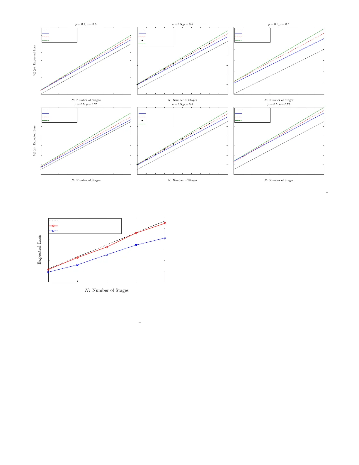
1 Optimal Adv ersarial Policies in the Multiplicati v e Learning System with a Malicious Expert S. Rasoul Etesami, Negar Kiya v ash, V incent Leon, and H. V incent Poor Abstract —W e consider a lear ning system based on the con ven- tional multiplicative weight (MW) rule that combines experts’ advice to predict a sequence of true outcomes. It is assumed that one of the experts is malicious and aims to impose the maximum loss on the system. The loss of the system is naturally defined to be the aggregate absolute differ ence between the sequence of predicted outcomes and the true outcomes. W e consider this problem under both offline and online settings. In the offline setting where the malicious expert must choose its entire sequence of decisions a priori, we show somewhat surprisingly that a simple greedy policy of always reporting false prediction is asymptotically optimal with an approximation ratio of 1 + O ( q ln N N ) , where N is the total number of prediction stages. In particular , we describe a policy that closely resembles the structure of the optimal offline policy . For the online setting where the malicious expert can adaptively make its decisions, we show that the optimal online policy can be efficiently computed by solving a dynamic program in O ( N 3 ) . Our results provide a new direction for vulnerability assessment of commonly-used learning algorithms to adversarial attacks where the threat is an integral part of the system. I . I N T R O D U C T I O N The focus of the vast literature on learning with e xpert advice is coming up with good prediction rules for the learning system even for the worst possible outcome sequence [1]–[6]. Howe ver , the proposed algorithms are not designed to be robust against malicious strategic experts. Given the prev alence of machine learning algorithms and as a result, automated decision making in distributed settings in many real-world applications, the effect of malicious experts whose goal is to destroy the performance of the system by injecting false predictions cannot be ignored. In this paper, we address this issue by analyzing the performance of the multiplicative weighted (MW) learning algorithm [3], widely used in collab- orativ e filtering, in the presence of malicious experts injecting false recommendations. There are many moti vating examples for considering the effect of malicious experts in real-world learning systems. T o name a few , one can consider movie recommendation systems such as IMDB or Netflix where the system relies on the users’ feedback (e xperts) to rate the quality of the movies. Howe ver , the users do not always report the true ratings due to various S. Rasoul Etesami and V incent Leon are with Department of Industrial and Enterprise Systems Engineering, Univ ersity of Illinois at Urbana-Champaign, Urbana, IL, 61801 email: (etesami1,jliang38)@illinois.edu. Negar Kiyavash is with College of Management of T echnology , Ecole polytechnique fdrale de Lausanne (EPFL), Lausanne, Switzerland (email: negar .kiyav ash@epfl.ch). H. V incent Poor is with Department of Electrical Engineering, Princeton Univ ersity , Princeton, NJ, 08540 (email: poor@princeton.edu). reasons such as manipulating the outcome of the system tow ard their preferences [6], [7]. As another e xample, one can consider sensor fusion in networks where a malicious sensor can attempt to attack the system by injecting false signals and cause the central decision-maker to reach incorrect decisions [8]. Moreover , almost all cases of collaborativ e filtering or distributed decision making are vulnerable to such internal threats. In this paper , we study the performance of the MW learning algorithm against adversarial attacks where the adversary’ s goal is to attack the system without ha ving control ov er the system’ s prediction rule. The MW update rule is one of the most commonly used schemes for learning from e xpert advice [1], [9], [10], in which after each stage of prediction, when the true outcome is re vealed, depending on whether the e xperts were correct or wrong on that stage, the system punishes or rew ards the experts, respectiv ely , by decreasing or increas- ing their relativ e weights by a multiplicativ e factor . Thus, learning with expert advice can be modeled in a multistage sequential decision-making framework where at each stage, the recommendation system combines the predictions of a set of experts about an unknown outcome with the aim of accurately predicting that outcome. The problem that we consider here was originally proposed in [11] and subsequently studied in [8], where it was shown that in the case of logarithmic loss function the optimal online policy for the malicious expert is a simple greedy policy . This, howe ver , is not quite surprising as the malicious expert’ s gain by reporting false predictions substantially dominates his credibility loss due to the logarithmic nature of the loss function. As it w as sho wn using numerical analysis in [8], [11], characterizing the optimal policy for the absolute loss function (which is the more interesting case and commonly used in MW learning systems) is much more challenging due to the strong coupling between the gain in reporting false prediction and the loss in credibility . In this work, we answer this question by sho wing that the same simple greedy algorithm is asymptotically optimal in the offline setting. Moreov er , we show that although the optimal online policy can hav e a complicated structure, it can still be computed efficiently using a reduced-size dynamic program. The problem that we study in this paper also belongs to the general family of many problems such as target tracking, distributed detection under the byzantine attacks, Sybil attack, and causati ve attack from the taxonomy of adversarial machine learning where the attacker can modify the data in the training or during the operation in order to degrade the performance of a machine learning algorithm [12]–[15]. Our work is also 2 related to [16]–[18] in which a learner plays against an adver - sary such that at each step the learner has to choose an expert from a pool of experts to follo w while the adversary adaptiv ely sets the gains for the experts with the aim of maximizing the overall regret incurred by the learner . The authors in [17] fully characterize the optimal online policies for the learner and the adversary in the case of 2 and 3 experts and provide some general insights into how to design an optimal algorithm for the learner and the adversary for an arbitrary number of experts. Ho wev er , our work is different from those in the sense that the experts in our setting are themselves malicious and can act strategically . Moreover , the performance guarantee in our setting is in terms of the approximation factor rather than the con ventional notion of re gret . W e consider the problem of learning with a malicious strategic expert under both of fline and online settings. More specifically , we consider a system with two experts; one honest and the other malicious. At each round, the honest expert predicts the true outcome with some accuracy , while the malicious expert strate gically provides a prediction with the goal of maximizing the loss incurred by the system. W e assume that the adversary kno ws the true outcome and prediction rule of the learning system. For the offline setting, we assume that the adversary reports his entire sequence of predictions at the beginning of the horizon, while for the online setting, the adversary is allowed to look at the past information up to the current stage and then reports his ne xt prediction. The problem that we address in this paper is two-fold: From the malicious expert’ s point of view , we are interested in knowing the optimal policy which imposes the maximum loss on the learning system, while from the system designer’ s point of view we are interested in knowing how the widely- applied MW learning algorithm performs in the presence of a malicious expert. As one of our main results we show that for the case of absolute loss function, the optimal offline policy can be approximated within a factor 1 + O ( q ln N N ) of the one which reports false predictions at all the stages, where N is the total number of prediction stages. This can be viewed as a counterpart for the con ventional regret minimization bounds obtained for the MW update rule. Here it is worth noting that obtaining such an approximation ratio is more challenging than obtaining regret bounds commonly used in expert advice settings. This is because the space of feasible policies is exponentially larger than the set of feasible actions. Therefore, for the of fline setting, we approximate the of fline policy rather than the action . One implication of our analysis under the of fline setting is that the commonly used MW learning algorithm is not robust with respect to adversarial attacks as a naiv e malicious expert can impose almost the same loss as an optimally strategic malicious expert. W e then extend our results to the online setting and formulate the optimal policy of an online adaptiv e adversary using a dynamic program (DP). In particular , we show that the number of states of this dynamic program grows only linearly in terms of the number of stages which allows us to compute the optimal online policy for the malicious expert efficiently in O ( N 3 ) . The paper is organized as follows: In Section II, we in- troduce the model formally and discuss some of its salient properties. In Section III, we provide our main results for the case of offline malicious expert and absolute loss function. In Section IV, we pro vide an efficient algorithm for computing the optimal online policy for the case of two experts, with an extension for the case of multiple honest experts. Simulation results for of fline and online adversaries are pro vided in Section V. W e conclude the paper by identifying some future directions of research in Section VI. I I . P RO B L E M F O R M U L A T I O N In this section, we first introduce the mathematical model formally as in [11], and then pro vide some of its salient properties which will be used in our later analysis. In the remainder of this paper , we shall refer to the ill-intent expert as a malicious expert or an adversary , interchangeably . Consider a learning system with two experts. At each round k = 0 , 1 , 2 , . . . , expert i ∈ { 1 , 2 } has a nonnegati ve weight denoted by p i k ∈ [0 , 1] . W e assume that both e xperts start with equal initial weight p 1 0 = p 2 0 = 1 . W e denote the prediction of the i th expert at stage k by x i k ∈ { 0 , 1 } , and the true outcome by y k ∈ { 0 , 1 } . At stage k , the relativ e weight of expert i ∈ { 1 , 2 } is defined to be ˜ p i k := p i k p 1 k + p 2 k . (1) In the k th stage, the learning system predicts the true outcome y k using a weighted av erage rule gi ven by ˆ y k = ˜ p 1 k x 1 k + ˜ p 2 k x 2 k , (2) and updates the experts’ weights in the next time step depending on whether they were correct or wrong in the previous instance using the following multiplicativ e weight (MW) update rule: p i k +1 = ( p i k  if x i k 6 = y k , p i k if x i k = y k . (3) Here  ∈ (0 , 1) is a fixed constant parameter set the learning system and reflects its aggressiv eness on punishing/rewarding the experts. W e note that the MW update rule (3) has been extensi vely used in the past literature [3], [10], [19], [20]. In particular , the MW learning system serves as an independent forecaster (e xecutor). Unlik e the adv ersary , the learning system is neither strategic nor has access to the information of the true outcomes: it merely tak es the e xperts’ advice and computes the prediction in each round using (2). After the true outcome y k is re vealed, the system incurs a loss l ( ˆ y k , y k ) = Q ( | ˆ y k − y k | ) , where Q ( · ) : [0 , 1] → R ≥ 0 can be some general nondecreasing function. In this paper , we shall only focus on the absolute loss function Q ( y ) := y , as it is the most common loss function used in the literature for the expert advice setting [3], [10]. W e assume that expert 2 is the honest e xpert who makes a correct prediction with accuracy µ , i.e., the one that agrees with the true outcome with probability µ : x 2 k = ( y k w .p. µ, 1 − y k w .p. 1 − µ. 3 Remark 1. F or asymmetric accuracies { µ k } k ∈ [ N ] , one can partition the horizon into epochs of a small constant length. As predictions of the honest expert ar e independent, one may assume that the honest expert’ s expected accuracy within each epoch is close to its expected value denoted by µ . Ther efor e, our analysis can be viewed as a constant appr oximation of the heter ogeneous model in the stationary r egime . Expert 1 is the malicious expert (adv ersary) who aims to impose the maximum loss on the system by taking the best adversarial action at each stage. W e assume that expert 1 knows the true outcome y k at time k ∈ [ N ] := { 1 , . . . , N } , as well as the distribution of x 2 k , the prediction of expert 2. 1 One of our main objectiv es in this paper is to e valuate the robustness of the MW learning algorithm in the presence of a malicious expert. For that reason, we ev aluate the system’ s performance against the most adverse scenario where the adversary has full information about the sequence of outcomes. W e refer to Proposition 3 for a weaker adversary with no information about an arbitrary sequence of true outcomes. Definition 1. A malicious expert is called an offline adversary if he c hooses his entir e of sequence of pr edictions { x 1 k } N k =1 at the be ginning of the horizon and then commits to it. A malicious expert is called an online adversary if the entir e history of pr edictions and true outcomes { ˜ p 1 ` , x 1 ` , x 2 ` , y ` } k − 1 ` =1 ar e available to him, and then he decides x 1 k . Finally , the goal of the malicious e xpert (either offline or online) is to produce a sequence of predictions { x 1 k } N k =1 ov er a fixed finite horizon N in order to maximize the expected aggregate loss on the system giv en by: E x 2 1 ,...,x 2 N [ N X k =1 l ( ˆ y k , y k )] = N X k =1 E x 2 1 ,...,x 2 k [ l ( ˆ y k , y k )] , (4) where the second e xpectation is taken o ver the past and current actions of the honest agent x 2 1 , . . . , x 2 k . In particu- lar , an optimal policy for the of fline/online malicious ex- pert is a sequence of decisions which maximizes the ob- jectiv e function (4) with respect to its corresponding in- formation set, i.e., a solution to the maximization problem max x 1 1 ,...,x 1 N P N k =1 E x 2 1 ,...,x 2 k [ l ( ˆ y k , y k )] . It is worth noting that one of the major dif ferences between the above model and the con ventional expert advice problem is that in the latter one assumes that all the experts are honest and simply report their true recommendations. In particular , the goal is to devise a learning scheme which combines the experts’ recommendations in an intelligent manner to accurately predict the unknown outcomes, where it can be shown that the well-known MW learning rule achieves the minimum regret bound. Howe ver , the above adversarial model can be viewed as a dual to the expert advice problem where the MW rule is fixed as the underlying learning process and the goal to ev aluate how well this learning rule will perform in the presence of a malicious expert who strate gically aims to maximize the loss of the system. 1 Note that the assumption that the adversary knows the prediction accuracy µ is not very restrictive as the adversary can always learn this distribution using the empirical history of observed actions taken by the honest expert. A. Pr eliminary Results Here, we describe some of the important properties of the aforementioned adversarial model which will be used later to establish our main results. First we note that using the update rule (3) and the definition of relative weights (1), we have ˜ p 1 k +1 =            1 1+  1 ˜ p 1 k − 1  1  if x 1 k = 1 − y k , x 2 k = y k , 1 1+  1 ˜ p 1 k − 1   if x 1 k = y k , x 2 k = 1 − y k , ˜ p 1 k if x 1 k = x 2 k , (5) In particular , from (5) one can easily see that the adversary’ s relativ e weight changes only when his prediction is at odds with the prediction of the honest agent (when both experts predict the same, the adversary’ s relati ve weight remains unchanged). As the update rule in (5) plays an important role in our analysis, we define a weight update function g : (0 , 1] → (0 , 1] and its in verse g ( − 1) : (0 , 1] → (0 , 1] by g ( ρ ) := 1 1 +  1 ρ − 1  1  , g ( − 1) ( ρ ) := 1 1 +  1 ρ − 1   . (6) In fact, both g ( ρ ) and its inv erse g ( − 1) ( ρ ) are strictly increas- ing functions and we have g ( ρ ) ≤ ρ ≤ g − 1 ( ρ ) , ∀ ρ ∈ (0 , 1] . An important feature of the functions g ( ρ ) and g ( − 1) ( ρ ) is that for any integer j ∈ Z + , we have g ( j ) ( ρ ) : = g ( . . . ( g ( ρ )) | {z } j times = 1 1 +  1 ρ − 1  1  j , g ( − j ) ( ρ ) : = g ( − 1) ( . . . ( g ( − 1) ( ρ )) | {z } j times = 1 1 +  1 ρ − 1   j , (7) where g ( j ) ( ρ ) and g ( − j ) ( ρ ) denote the composition of g ( ρ ) and g ( − 1) ( ρ ) by themselves j times, respecti vely . In particular , we note that g (0) ( ρ ) ≡ ρ . I I I . O P T I M A L O FFL I N E P O L I C Y F O R T H E A B S O L U T E L O S S F U C T I O N In this section, we analyze the optimal policy for the of fline adversary and postpone our analysis for the case of the online adversary to Section IV. W e recall that the offline adversary is the one who chooses his entire sequence of decisions (predictions) at the beginning of the horizon. More precisely , the of fline adv ersary aims to maximize the e xpected loss of the learning system given by (4) ov er all the 2 N feasible sequences of the form { 0 , 1 } N . Note that although the space of feasible solutions is exponentially lar ge, howe ver we are only interested in obtaining polynomial-time computable policies. Therefore, our goal here is to approximate the optimal offline policy within only a ne gligible additiv e error term in the ov erall objecti ve cost. T oward this end, we first establish a sequence of lemmas to prov e our main approximation result (Theorem 1). In fact, many of these lemmas do not make an y use of the specific 4 structure of the functions g ( ρ ) and Q ( · ) , and we state them in a more general form. Later , in order to provide more closed- form approximation results, we specialize these lemmas to the specific choice of g ( ρ ) gi ven in (6) and linear loss function Q ( y ) = y . It is worth noting that although we assumed that the learning algorithm starts with equal initial weight for both experts (i.e., the initial relati ve weight of the adversary is 0 . 5 ), howe ver , we state our results for an offline adversary with generic initial relativ e weight ρ . The reason for this choice would become apparent subsequently . Next, we state the following lemma from [8, Lemma 1] whose proof is by induction on the horizon length N . Lemma 1. F or a loss function l ( ˆ y , y ) = Q ( | ˆ y − y | ) , with Q : [0 , 1] → R ≥ 0 , the expected loss given in (4) is fully determined by the initial relative weight of the adversary ρ , his policy Ψ := ( x 1 1 , . . . , x 1 N ) ∈ { 0 , 1 } N , and the horizon length N . From Lemma 1 one can see that the adversary can tak e his optimal actions by only adjusting them relative to the honest expert’ s actions. Henceforth, the expected loss in (4) for a giv en policy Ψ = ( x 1 1 , x 1 2 , . . . , x 1 n ) of the offline adversary can be represented by V Ψ n ( ρ ) := P n k =1 E x 2 1 ,...,x 2 k [ l ( ˆ y k , y k )] , where ρ denotes the initial relati ve weight of the adversary . Definition 2. Assume the adversary’ s initial weight is ρ and the number of stages is n . An adver sary’ s policy is called a false policy if he lies in all the stages, i.e ., x 1 k = 1 − y k , ∀ k ∈ [ n ] . It is called a true policy if the adversary tells the truth in all the stages, i.e., x 1 k = y k , ∀ k ∈ [ n ] . W e let V f n ( ρ ) and V t n ( ρ ) denote the expected loss of the system if the adversary follows the false policy and the true policy , respectively . Using the above definition we can obtain closed-form rela- tions for the expected loss of the f alse/true policies as giv en in the follo wing lemma. W e will use these expressions as black- boxes in our approximation analysis. Lemma 2. F or a loss function l ( ˆ y , y ) := Q ( | ˆ y − y | ) , initial adversary’ s weight ρ , and n stages, we have V f n ( ρ ) = n (1 − µ ) Q (1) + n X j =0 P ( Z > j ) Q ( g ( j ) ( ρ )) , V t n ( ρ ) = nµQ (0) + n X j =0 P ( W > j ) Q (1 − g ( − j ) ( ρ )) , wher e Z ∼ B in ( n, µ ) and W ∼ B in ( n, 1 − µ ) ar e Binomial distributions with parameter s µ and 1 − µ , respectively . Pr oof. Let us fix the adversary’ s policy to the false policy , and we look at all the possible sample paths which can be realized by predictions of the honest expert. An y sample-path in which the honest e xpert predicts correctly i times and makes a mistake n − i times will occur with the same probability of µ i (1 − µ ) n − i . There are exactly  n i  of such sample paths, and for any of such sample paths, independent of what positions the honest expert predicts correctly or wrongly , the incurred loss giv en the fixed adversary’ s false policy equals to ( n − i ) Q (1) + P i − 1 j =0 Q ( g ( j ) ( ρ )) . This is because, for any of n − i false predictions of the honest agent in this sample-path, the system incurs a loss of Q (1) and by (5) the relati ve weight of the adv ersary does not change. Moreov er , for the remaining i correct predictions and regardless of their order , the system incurs a loss of P i − 1 j =0 Q ( g ( j ) ( ρ )) (note that for i = 0 this term equals to 0). Therefore, by taking an expectation ov er all possible sample paths we hav e, V f n ( ρ ) = n X i =0  n i  µ i (1 − µ ) n − i ( n − i ) Q (1) + n X i =0  n i  µ i (1 − µ ) n − i i − 1 X j =0 Q ( g ( j ) ( ρ )) = n (1 − µ ) Q (1) + n X i =0 i − 1 X j =0  n i  µ i (1 − µ ) n − i Q ( g ( j ) ( ρ )) = n (1 − µ ) Q (1) + n − 1 X j =0 n X i = j +1  n i  µ i (1 − µ ) n − i Q ( g ( j ) ( ρ )) = n (1 − µ ) Q (1) + n X j =0 P ( Z > j ) Q ( g ( j ) ( ρ )) , where in the last equality we have used the fact that Z ∼ B in ( n, µ ) and P ( Z > n ) = 0 . Similarly , to compute V t n ( ρ ) we can fix the adv ersary’ s policy to the true policy . Now for any sample-path realized by the hon est expert with i correct predictions, the system incurs a loss of i · Q (0) + P n − i − 1 j =0 Q (1 − g ( − j ) ( ρ )) . Finally , taking an expectation ov er all sample paths we get V t n ( ρ ) = n X i =0  n i  µ i (1 − µ ) n − i i · Q (0) + n X i =0  n i  µ i (1 − µ ) n − i n − i − 1 X j =0 Q (1 − g ( − j ) ( ρ )) = nµQ (0) + n − 1 X j =0 n − j − 1 X i =0  n i  µ i (1 − µ ) n − i Q (1 − g ( − j ) ( ρ )) = nµQ (0) + n X j =0 P ( W > j ) Q (1 − g ( − j ) ( ρ )) , where the second equality is by switching the order of sum- mations, and the last equality is by W ∼ B in ( n, 1 − µ ) . Next, we note that ev ery offline policy can be parti- tioned into sev eral blocks such that within each block the adversary follows either false or true policies. Thus we can characterize any offline policy by simply determining the length of each of its sub-blocks. For this purpose, let n 1 , m 1 , n 2 , m 2 , . . . , n k , m k , denote the partition of the entire horizon N into some sub-horizons of integer length for some positiv e integer k such that N = P k i =1 ( n i + m i ) , and m i , n i ∈ Z + (note that n 1 or m k can also be zero). W e assume that the adversary follows the false policy within each block of length n i , and the true policy within each block of length m i . Therefore, finding the optimal offline policy reduces to maximizing the expected loss (4) over all such partitions. Lemma 3. Given an adversary’ s initial relative weight ρ , the r elative weight of the adversary after lying n times and telling truth m times (in any arbitrary or der) equals to 5 g ( X − Y ) ( ρ ) , wher e X ∼ B in ( n, µ ) and Y ∼ B in ( m, 1 − µ ) ar e independent Binomial random variables. Pr oof. Let ¯ X i ∼ B er ( µ ) and ¯ Y i ∼ B er (1 − µ ) , i = 1 , 2 , . . . be independent Bernoulli random v ariables, and ρ be the initial weight of the adversary . Since at each stage the honest expert predicts independently from the earlier stages, a simple induction shows that if the adversary’ s weight at the beginning of the k th stage equals to g ( U ) ( ρ ) for some random v ariable U , then after the k th stage depending on whether he lies or tells the truth, his weight will change to g ( U + ¯ X k ) ( ρ ) or g ( U − ¯ Y k ) ( ρ ) , respectiv ely . Therefore, if we know that the adversary lies exactly n times and tells the truth m times, his relativ e weight at the end of this process will be equal to g ( X − Y ) ( ρ ) , where X is the sum of n independent Bernoulli random variables of type ¯ X i ∼ B er ( µ ) , and Y is the sum of m independent Bernoulli random variables of type ¯ Y i ∼ B er (1 − µ ) . This implies that X ∼ B in ( n, µ ) and Y ∼ B in ( m, 1 − µ ) , and that X and Y are independent. Lemma 3 indicates that the distribution of the adversary’ s relativ e weight, induced by following an offline policy Ψ , only depends on the total number of times that the adversary lies or tells the truth, and not on the specific order of them. Note that this property only holds for the relativ e weight distribution, b ut not for the distribution of the accumulated loss at different stages. In fact, it can be sho wn that the distribution of loss depends critically on the order of the adversary’ s actions, and that is the main difficulty in the analysis of the optimal offline policy . W e circumvent this issue in the follo wing theorem by providing an approximation scheme that is asymptotically optimal as the number of stages approaches infinity . Theorem 1. F or any  ∈ (0 , 1) , and the absolute loss function l ( ˆ y , y ) = | ˆ y − y | , we have V Ψ ∗ N (0 . 5) V f N (0 . 5) = 1 + O ( q log 1 / N N ) , wher e V Ψ ∗ N (0 . 5) and V f N (0 . 5) denote the expected loss by following the optimal policy and the false policy , r espectively . Pr oof. For simplicity and without any loss of generality we set  = 1 e . For general  ∈ (0 , 1) , the only dif ference in our analysis would be that the base of the natural logarithm will change to 1  . Using Lemma 2 specialized for the absolute loss function Q ( y ) = y , we can write V f n ( ρ ) = (1 − µ ) n + n X j =0 P ( Z > j ) g ( j ) ( ρ ) , V t n ( ρ ) = (1 − µ ) n − n X j =0 P ( W > j ) g ( − j ) ( ρ ) , (8) where Z ∼ B in ( n, µ ) and W ∼ B in ( n, 1 − µ ) . For any arbitrary b ut fixed ρ ∈ (0 , 1) , let us define f ( r ) := r − ln(1 + ae r ) ,  ( r ) := f ( r + 1) − f ( r ) − g ( r ) ( ρ ) , where a := 1 ρ − 1 and r ∈ [0 , ∞ ) . Now we can write, V f n ( ρ ) = (1 − µ ) n + n X j =0 P ( Z > j )[ f ( j + 1) − f ( j ) −  ( j )] = (1 − µ ) n − n X j =0 P ( Z > j )  ( j ) + n X j =0 [ P ( Z > j − 1) − P ( Z > j )] f ( j ) − f (0) = (1 − µ ) n − n X j =0 P ( Z > j )  ( j ) + E [ f ( Z )] − f (0) (a) ≤ (1 − µ ) n + E [ f ( Z )] − f (0) − n X j =0 P ( Z > j )  1 1 + ae j +1 − 1 1 + ae j  (b) = (1 − µ ) n + E [ f ( Z )] − f (0) + g (0) ( ρ ) − E [ g ( Z ) ( ρ )] (c) = n − E [ln(1 + ( 1 ρ − 1) e Z )] − ln( ρ ) + ρ − E [ 1 1 + ( 1 ρ − 1) e Z ] , (9) where ( a ) is due to Lemma 4 (Appendix A) which shows that  ( r ) ≥ 1 1+ ae r +1 − 1 1+ ae r , and ( b ) follows from (7) and the definition of e xpectation. Finally , ( c ) follows by substituting the expressions for f ( Z ) and g ( Z ) ( ρ ) . Similarly , to obtain an upper bound for V t n ( ρ ) , let us define h ( r ) := ln( a + e r ) , δ ( r ) := h ( r + 1) − h ( r ) − g ( − r ) ( ρ ) . Using identical steps as in the deriv ation of (9) and since by Lemma 4, δ ( r ) ≤ 1 1+ ae − ( r +1) − 1 1+ ae − r , we get V t n ( ρ ) ≤ (1 − µ ) n − E [ln(( 1 ρ − 1) + e W )] − ln( ρ ) − ρ + E [ 1 1 + ( 1 ρ − 1) e − W ] . (10) Next let us consider an arbitrary offline polic y Ψ character- ized by its false/true sub-block, i.e., Ψ := n 1 , m 1 , . . . , n k , m k . Denote the expected loss under policy Ψ when the initial weight of the adversary w as 0 . 5 by V Ψ N (0 . 5) . Moreover , for ` = 1 , . . . , k , let ¯ X ` ∼ B in ( n ` , µ ) and ¯ Y ` ∼ B in ( m ` , 1 − µ ) be pairwise independent Binomial distributions (i.e., for ev- ery i and every j , ¯ X i and ¯ Y j are independent) and define X ` = P ` i =1 ¯ X i , and Y ` = P ` i =1 ¯ Y i . Note that the pair X ` and Y ` are independent Binomial distributions. By linearity of expectation, and using Lemma 3 we can write, V Ψ N (0 . 5) = V f n 1 (0 . 5) + E h V t m 1  g ( X 1 ) (0 . 5)  i + E h V f n 2  g ( X 1 − Y 1 ) (0 . 5)  i + E h V t m 2  g ( X 2 − Y 1 ) (0 . 5) i + . . . + E h V t m k  g ( X k − Y k − 1 ) (0 . 5)  i . (11) 6 Replacing g ( X ` − 1 − Y ` − 1 ) (0 . 5) (or for bre vity g ( X ` − 1 − Y ` − 1 ) ) from (7) instead of ρ in (9), and taking expectation we hav e E h V f n `  g ( X ` − 1 − Y ` − 1 ) i ≤ E  n ` − E h ln  1 + ( 1 g ( X ` − 1 − Y ` − 1 ) − 1) e Z  i  − E h ln  g ( X ` − 1 − Y ` − 1 ) i + E h g ( X ` − 1 − Y ` − 1 ) − E h 1 1 + ( 1 g ( X ` − 1 − Y ` − 1 ) − 1) e Z ii = n ` − E  ln  1 + e X ` − Y ` − 1 1 + e X ` − 1 − Y ` − 1  + E h 1 1 + e X ` − 1 − Y ` − 1 − 1 1 + e X ` − Y ` − 1 i , (12) where the equality follows by simplifying the terms and noting that for the ` -the false block Z := ¯ X ` ∼ B in ( n ` , µ ) , which is independent of X ` − 1 and Y ` − 1 . Similarly , since for the ` -th true block W := ¯ Y ` ∼ B in ( m ` , 1 − µ ) , which is independent of X ` and Y ` − 1 , by replacing g X ` − Y ` − 1 (0 . 5) instead of ρ into (10) and taking expectation we get E h V t m `  g ( X ` − Y ` − 1 ) (0 . 5) i ≤ (1 − µ ) m ` − E h ln  e X ` − Y ` − 1 + e ¯ Y ` 1 + e X ` − Y ` − 1 i + E h 1 1 + e X ` − Y ` − 1 1 + e X ` − Y ` − 1 i . (13) Finally , substituting (12) and (13) into (11), we can write V Ψ N (0 . 5) ≤ k X ` =1 ( n ` + (1 − µ ) m ` ) − E h k X ` =1  ln  e X ` − Y ` − 1 + e ¯ Y ` 1 + e X ` − Y ` − 1  + ln  1 + e X ` − Y ` − 1 1 + e X ` − 1 − Y ` − 1  i + 2 k X ` =1 E h 1 1 + e X ` − Y ` − 1 1 + e X ` − Y ` − 1 i = µM + (1 − µ ) N − E " ln k Y ` =1 e X ` − Y ` − 1 + e ¯ Y ` 1 + e X ` − 1 − Y ` − 1 !# + O ( √ N ln N ) = (1 − µ ) N − E  ln  1 + e Y k − X k 2   + O ( √ N ln N ) = (1 − µ ) N + O ( √ N ln N ) , (14) where the first equality is due to Lemma 8 (Appendix A) and noting that P k ` =1 n ` = M and P k ` =1 m ` = N − M . Moreov er , the second equality holds because ¯ Y ` = Y ` − Y ` − 1 (which causes telescopic cancellation of the product terms inside of the natural logarithm) and noting that X 0 = Y 0 = 0 , E [ X k ] = µM . Using (8), the expected loss of the false policy is at least, V f N (0 . 5) = (1 − µ ) N + N X j =0 P ( Z > j ) g ( j ) (0 . 5) ≥ (1 − µ ) N . (Note that all the terms P ( Z > j ) g ( j ) (0 . 5) are nonnegati ve.) This in vie w of (14) sho ws that V Ψ ∗ N (0 . 5) V f N (0 . 5) = 1 + O ( q ln N N ) . Remark 2. It is important to distinguish the differ ence be- tween the appr oximation ratio obtained in Theor em 1 and the sub-linear r e gr et bounds commonly derived in re gr et minimization analysis. Her e we allow the offline malicious expert to choose his offline policy over the entire horizon (i.e., an arbitrary sequence of false/true pr edictions) and do not restrict him to his action (i.e., only select one action and commit to it at all the stages). Surprisingly , Theor em 1 shows that giving such an extr a power to the malicious expert does not bring him much gain other than a ne gligible additive term. Finally , we note that Theorem 1 suggests that the MW learning algorithm with absolute loss function is not very robust against malicious attacks. This is because the malicious expert does not to be very intelligent or hav e access to many computational resources to destroy the outcomes of the MW learning system; ev en following a simple false polic y can nearly impose the same loss as any other complex policy . A. Beyond Asymptotic Optimality for the Offline P olicy Theorem 1 shows that the false policy asymptotically achiev es the same performance as the optimal offline policy . Howe ver , the exact structure of the optimal offline policy for a finite horizon N can be quite complex. Therefore, our goal in this section is to take one step further and provide a polic y that closely resembles the structural patterns of the optimal offline policy . As it was sho wn in the proof of Theorem 1 one of the main reasons that there is a gap between the expected loss of the optimal offline policy and that of the false policy is the term: B := k X ` =1 E  1 1 + e X ` − Y ` − 1 1 + e X ` − Y ` − 1  henceforth referred to as the bonus term. Here, X ` ∼ B in ( N ` , µ ) and Y ` ∼ B in ( M ` , 1 − µ ) are independent Bino- mial distributions where N ` = P ` i =1 n i and M ` = P ` i =1 m i . Therefore, it seems reasonable to expect the optimal of fline policy (or a policy close to optimal), to maximize B in order to gain as much as possible from the bonus term. As such, we search the optimal offline policy Ψ ∗ among policies Ψ that satisfy the following two criteria: • i ) Ψ imposes at least as much loss as the false policy on the learning system, i.e., at least (1 − µ ) N − o (1) , • ii ) Ψ maximizes the bonus gain B . T o maximize the bonus term, using Lemma 8 (Appendix A), it is enough to maximize k X ` =1 h Φ( − µ 2 ` σ 2 ` ) − Φ( − µ 2 ` − 1 σ 2 ` − 1 ) i , (15) where Φ( · ) is the CDF of the standard normal distrib ution and µ 2 ` = N ` µ − M ` (1 − µ ) , σ 2 2 ` = µ (1 − µ )( N ` + M ` ) , µ 2 ` − 1 = N ` µ − M ` − 1 (1 − µ ) , σ 2 2 ` − 1 = µ (1 − µ )( N ` + M ` − 1 ) . Now by adjusting the ar gument of Φ( · ) in (15) to period- ically switch around 0 (see Figure 1), we obtain a positiv e gain from each of the summands in (15). This suggests that 7 Fig. 1. Mean and standard de viation adjustment for maximizing the bonus term B using CDF of the standard normal distribution. a policy in which − µ 2 ` σ 2 ` = 1 , and − µ 2 ` − 1 σ 2 ` − 1 = − 1 , would be a good candidate for maximizing the bonus term. Note that here the choice of 1 or − 1 is not strict and it can be replaced by any two points close to zero such that the difference of the normal CDF ev aluated at those points giv es a sufficiently large gain. Solving − µ 2 ` σ 2 ` = 1 and − µ 2 ` − 1 σ 2 ` − 1 = − 1 , by substituting the abov e expressions for µ 2 ` , σ 2 ` , σ 2 ` , σ 2 ` − 1 , we obtain a ratio type policy in which the ratio of the false/true block lengths n ` m ` , ` = 1 , 2 , . . . , is proportional to 1 − µ µ . Therefore, to fulfill both criteria ( i ) and ( ii ) , we introduce the following offline ratio policy: Definition 3. Let a and b be the smallest positive integ ers such that a b = µ 1 − µ . 2 W e say that ˆ Ψ is a ratio policy if its block r epr esentation is of the form ( n 1 , m 1 , . . . , m k − 1 , n k , m k ) = ( b, a, b, a, b, . . . , a, N 2 , 0) , wher e for ` = 1 , 2 , . . . , k , the adver- sary lies in n ` -blocks and tells the truth in m ` -blocks. T o verify why the ratio policy is indeed a good offline policy , let us denote the number of lies and truths in ˆ Ψ by M and N − M , respecti vely . Due to Definition 3, ˆ Ψ has many more lies than the truth in its structure (note that n k = N 2 ). Thus a similar analysis as in Lemma 2 for the false policy rev eals that the expected loss in ˆ Ψ which is obtained from its last block n k = N 2 is almost the same as the false policy minus a negligible constant which does not depend on N . As a result, the expected loss of ˆ Ψ which is obtained due to its heavy tail of false predictions is at least (1 − µ ) N − o (1) . On the other hand, the ratio polic y ˆ Ψ gains e xtra bonus due to its first N 2 stages. T o e valuate the bonus term B for the ration policy ˆ Ψ , we observe that due to Definition 3, µ 2 ` = 0 , and µ 2 ` − 1 = µb , for all ` ∈ [ k ] . Thus, for each ` ∈ [ k ] , we hav e Φ( − µ 2 ` σ 2 ` ) − Φ( − µ 2 ` − 1 σ 2 ` − 1 ) = Φ(0) − Φ( − µb σ 2 ` − 1 ) > 0 . In other words, each of these terms contributes positiv ely with some constant amount to the bonus B . Since we chose a and b as the smallest positi ve integers such that a b = µ 1 − µ , this assures that the number of summands k in the bonus term B (which equals the number of switching between false/true 2 Here for simplicity we have assumed that µ 1 − µ is a rational number , otherwise, we can always find positive integers such that a b ∼ = µ 1 − µ . blocks) is maximized. This is exactly why we defined our ratio policy the way we did in Definition 3. This shows that the expected loss of the ratio policy is at least as high as that for the false policy (satisfying criterion ( i ) ) with an additional bonus term B (satisfying criterion ( ii ) ). I V . O P T I M A L O N L I N E P O L I C Y F O R T H E A B S O L U T E L O S S F U N C T I O N In this section, we consider the problem of finding the optimal online policy for the malicious expert, where we recall that the online adv ersary is the one who chooses his next action adaptiv ely based on all the past rev ealed information up to the current stage. In order to be able to find the optimal online policy we first cast it as a dynamic program and then sho w that it can be solved efficiently in O ( N 3 ) . For this purpose, let us assume again that the malicious expert is expert 1 and the other expert is the honest one who makes a correct prediction with probability µ . W e assume that at stage k , expert 1 knows the true outcome y k , the accuracy µ of the honest expert, and the entire history of predictions up to stage k − 1 , i.e., { ˜ p 1 ` , ˜ p 2 ` , x 1 ` , x 2 ` , y ` : ∀ ` ∈ [ k − 1] } . Giv en this information set, the goal of the online malicious expert is to produce a sequence of predictions { x 1 k } N k =1 ov er a fixed finite horizon N to maximize the expected accumulated loss of the system gi ven by (4). Now let us define the state of the system at stage k to be the relati ve weight of the adversary at that stage, i.e., ˜ p 1 k . Note that as ˜ p 1 k + ˜ p 2 k = 1 , ∀ k , knowing ˜ p 1 k is sufficient to determine the relati ve weight of the honest expert ˜ p 2 k . Next let us define c x 1 k ( ˜ p 1 k ) to be the curr ent loss that the online adversary can impose on the system at stage k by taking the action x 1 k , i.e., c x 1 k ( ˜ p 1 k ) = E x 2 k [ | ˆ y k − y k || x 1 1 ] = ( 1 − µ + µ ˜ p 1 k if x 1 k = 1 − y k , (1 − µ )(1 − ˜ p 1 k ) if x 1 k = y k , (16) where the second equality is by Lemma 1 specialized to the absolute loss function Q ( y ) = y . W e can then cast the adversary’ s online optimal policy as a solution to an MDP in which the malicious expert’ s action at stage k imposes a current loss of c x 1 k ( ˜ p 1 k ) on the system and changes the state from ˜ p 1 k to the next state ˜ p 1 k +1 . In particular , the state transition of this MDP is giv en by the update rule (5), that is, ˜ p 1 k +1 =      g ( ˜ p 1 k ) if x 1 k = 1 − y k , x 2 k = y k , g ( − 1) ( ˜ p 1 k ) if x 1 k = y k , x 2 k = 1 − y k , ˜ p 1 k if x 1 k = x 2 k . (17) Now the solution to this MDP can be obtained using dynamic programming as shown in Algorithm 1. In this algorithm V ∗ k +1 ( · ) denotes the optimal value function, i.e., the optimally accumulated loss from time step k + 1 onward. In particular, from Lemma 1, one can easily see that the optimal v alue function does not depend on the sequence of true outcomes and is only a function of the state and the number of remaining stages. No w by substituting the closed form expressions of the current cost (16) and the state transition 8 Algorithm 1 DP Algorithm Initialize: V N ( · ) = c N ( · ) = 0 . For each step k = N − 1 do wnto 0 , find the optimal action x ∗ k := arg max x 1 k  c x 1 k ( ˜ p 1 k ) + E [ V ∗ k +1 ( ˜ p 1 k +1 )]  , and the optimal value function, V ∗ k ( ˜ p 1 k ) = max x 1 k  c x 1 k ( ˜ p 1 k ) + E [ V ∗ k +1 ( ˜ p 1 k +1 )]  . (19) Output: sequence x ∗ N − 1 , V ∗ N − 1 ( · ) , ..., x ∗ 0 , V ∗ 0 ( · ) . (17) into the DP Algorithm 1, and letting ρ := ˜ p 1 k for brevity , we obtain the following closed-form recursion for computing the optimal value function: V ∗ k ( ρ ) = max n 1 − µ + µρ + µV ∗ k +1 ( g ( ρ )) + (1 − µ ) V ∗ k +1 ( ρ ) , (1 − µ )(1 − ρ ) + (1 − µ ) V ∗ ( g ( − 1) ( ρ )) + µV ∗ k +1 ( ρ ) o , (18) where the first term in the maximization (18) corresponds to the adversary’ s action at stage k being x 1 k = 1 − y k , and the second term corresponds to the adversary’ s action being x 1 k = y k . Unfortunately , due to the nonlinear structure of the transition functions g ( ρ ) and g ( − 1) ( ρ ) , as well as their joint con vex/conca ve structure, solving the recursion (18) in a closed-form seems to be a tedious task. Although at each stage of the above recursion one needs to consider the maximum of two alternatives (so that the number of alternati ves will grow exponentially in terms of the number of stages), howe ver , in the following theorem we show that most of these alternativ es collapse on each other so that the optimal v alue function in (18) can be computed efficiently in polynomial time. Theorem 2. The optimal policy for the online malicious e xpert can be found in O ( N 3 ) , wher e N is the number of stages. Pr oof. Let us consider a decision tree with a root node representing the initial relati ve weight of the adversary (i.e., ρ = 0 . 5 ) and such that the nodes in the k -th level of the tree that are at distance k from the root represent all the possible relativ e weights of the adversary after k stages (Figure 2). The ke y observ ation is that due to the property of g ( · ) and its in verse g ( − 1) ( · ) , the size of this decision tree does not grow exponentially such as a binary tree. In fact, a simple induction shows that the nodes in the k -th lev el of the tree can be grouped to form exactly 2 k − 1 nodes representing all possible relativ e weights of the adversary up to stage k , given by g ( − k ) (0 . 5) , g ( − k +1) (0 . 5) , . . . , g ( k − 1) (0 . 5) , g ( k ) (0 . 5) . 3 There- fore, the total number of tree nodes by such grouping (states in the DP) after N stages is at most P N k =1 (2 k − 1) = O ( N 2 ) . As a result, solving the dynamic recursion (18) backward by moving from the tree lea ves toward the root, the number of computations to find the optimal online policy using the DP recursion (18) is at most O ( N × N 2 ) . 3 Using Lemma 3, one can e ven compute the distrib ution of the weights on the reduced nodes efficiently using Binomial distributions. Fig. 2. Illustration of the first le vel (root) and the second level of the decision tree. The top actions connecting the root to the intermediate black circles correspond to the honest expert’ s decisions. The bottom actions connecting the black circles to the second level of the tree correspond to the malicious expert’ s decisions. Although the second level originally has four nodes, howe ver , two of them can be grouped and be reduced to only three states. The weights on the dashed paths simply denote the loss of the system by following that path. Finally , in a recent work [21], the authors hav e analyzed the DP (18) in more detail by providing upper and lower bounds on the optimal value function using the approximated dynamic program’ s viscosity solution. More precisely , it was shown in [21] that for any online policy Ψ for the malicious expert: lim sup N →∞ V ∗ 0 (0 . 5) N ≤ 1 − µ 2 , lim inf N →∞ V ∗ 0 (0 . 5) N > 1 − µ. A. A Generalization to Multiple Experts Here we provide a generalization of the problem to the case of many honest experts and one adversary . W ithout loss of generality , we again assume that the malicious expert is expert 1 and that all the other experts i ∈ { 2 , . . . , K } are honest who make a correct prediction with different probabilities µ i (the accuracy of expert i ). That is, x i k =  y k w .p. µ i , 1 − y k w .p. 1 − µ i . W e assume that at round k , expert 1 kno ws the true outcome y k , the accuracy of the honest experts, and the whole history of predictions up to round k − 1 , i.e., { ˜ p j ` , x j ` , y ` : ∀ ` ∈ [ k − 1] , j ∈ [ K ] } . Giv en this information set, the goal of the online malicious expert is to produce a sequence of predictions { x 1 k } N k =1 ov er a fixed finite horizon N in order to maximize the expected accumulated loss of the system, max x 1 1 ,...,x 1 K E x i k ,k ∈ [ N ] ,i 6 =1  N X k =1 l ( ˆ y k , y k )  , where the expectation is taken over the randomization of all the honest e xperts’ predictions { x i k , k ∈ [ N ] , i 6 = 1 } . W e let ~ p k = ( p 1 k , p 2 k , ..., p K k ) be the state or weight vector of all e x- perts at round k and ~ ˜ p k = ( ˜ p 1 k , . . . , ˜ p K k ) be the corresponding normalized weight vector where ˜ p i k = p i k P i ∈ [ K ] p i k , i ∈ [ K ] is the normalized weight of expert i . Note that we always have 9 P i ∈ [ K ] ˜ p i k = 1 , ∀ k . Moreover , we let φ x 1 k ( ~ p k ) be the state transition at stage k giv en that the online malicious expert takes the action x 1 k ∈ { 0 , 1 } , i.e., φ x 1 k ( ~ p k ) =  p 1 k +1 , . . . , p K k +1  , where p i k +1 = p i k  l ( x i k ,y k ) . In addition, the learning algorithm predicts ˆ y k at time k by ˆ y k = P i ∈ [ K ] p i k x i k P i ∈ [ K ] p i k = X i ∈ [ K ] ˜ p i k x i k . W e note that for K = 2 , this generalized setting coincides with that giv en in Section II. Although characterizing the structure of the optimal online policy in the generalized setting can be very complicated, in the next section we provide some numerical experiments to study the beha vior of the optimal policy with multiple honest experts. V . S I M U L A T I O N S Performance of the false, ratio, and optimal online policies has been simulated numerically and compared in Figure 3. In addition to offline and online policies, the case of no adversary with two identical honest experts has also been simulated in order to show the effect of an adversary in the system. As can be seen in all plots, an adversary simply adopting the false policy incurs extra loss compared to a system where a malicious expert is not present. The ratio polic y imposes more loss than the false policy when the number of stages is lar ge. The optimal online policy imposes a strictly greater loss than the optimal offline policy . Moreov er , as the number of stages increases, the gap between the loss of the optimal online polic y and either of the offline policies also increases. Similarly , the gain of the bonus term B , which is the difference between the curves of the false policy and the ratio polic y , increases as the number of stages increases. In fact, it can be observed that the ratio policy closely mimics the structure of the optimal offline policy . F or instance, in the middle subfigures of Figure 3, the optimal of fline expected loss for sev eral values of N = 10 , 12 , 14 , 16 , 18 , 20 , 22 , 24 , 26 are plotted using black dots. As these values are very close to the expected loss of the ratio policy and ev en coincide in certain cases (e.g., N = 10 , 14 , 16 ), we believ e that the optimal of fline policy for finite N belongs to the class of ratio policies, giv en that one could properly round the block lengths using the CDF of normal distribution. Finally , using the generalization to multiple experts in Sec- tion IV, a system with four honest experts and one adversary is simulated and compared to a system with one honest expert and one malicious expert. In the 5-expert model, all experts hav e identical initial weights. In the 2-expert model, the adversary’ s initial relativ e weight is ρ = 0 . 2 , which is the same as that in the 5-e xpert model. The accuracy of the honest expert in the 2-expert model is the mean of the four honest experts’ accuracy in the 5-e xpert model. T wo cases are considered: the homogeneous case (accuracies of all honest experts are identical, µ 2 = µ 3 = µ 2 = µ 5 = 0 . 5 ) and the heterogeneous case (accuracies of honest experts are distinct, µ 2 = 0 . 3 , µ 3 = 0 . 4 , µ 4 = 0 . 6 , µ 5 = 0 . 7 ). The mean of the accuracies of honest experts is the same for the two cases. Expected loss for the 5-expert model is estimated as follows. In each play , a sequence of actions { 0 , 1 } N is randomly generated for each honest expert i ∈ { 2 , 3 , 4 , 5 } according to his accuracy µ i , and the adversary chooses his optimal policy against the honest experts’ strategies. This process is repeated 100 times, and the expected loss is approximated by the empirical mean of the losses for all the 100 plays. Numerical results are shown in Figure 4. As the curve for the homogeneous 5-expert model is very close to that for the 2-expert model, it suggests that the 2-expert model can well approximate the system with multiple homogeneous honest experts by replacing all honest experts with a single one of combined relati ve weight and the same accuracy . The difference between the curves for the 2-expert model and the heterogeneous 5-expert model is greater , probably because the optimal online policy in the generalized heterogeneous setting is dif ficult to be approximated by only 2-experts. V I . C O N C L U S I O N S A N D F U T U R E D I R E C T I O N S In this paper , we considered an adversarial learning system with two experts of whom one is malicious. The malicious expert aims to impose the maximum loss on the system by strategically reporting f alse predictions. W e analyzed the optimal policy for the malicious e xpert under both offline and online settings. In the of fline setting, we showed that finding the optimal policy for the adversary is essentially a hard discrete optimization problem whose solution can be approximated within a negligible (sub-linear) additive term. In particular , we provided a more refined polic y that closely mimics the behavior of the optimal of fline policy . W e then considered the optimal policy for the online malicious expert and sho wed that it can be ef ficiently computed using a dynamic program, and generalized the setting to multiple experts. This work opens many interesting directions for future research. It would be interesting to see whether the structure of the optimal policy for the online adversary can be charac- terized in a closed-form. One possible direction is to lev erage the dynamic recursion (18) to show that the optimal value function possesses some nice properties such as conv exity , which allo ws us to prove a class of optimal threshold policies for the online adversary [22]. Another interesting direction is to use learning schemes other than the MW algorithm (e.g., upper confidence bound algorithm) as the underlying learning scheme and study their robustness against adversarial attacks. When there are man y e xperts in the system can we use mean- field approximation as an effecti ve tool to approximate the optimal policies? Finally , it is interesting to study the game- theoretic v ersion of this work in which the MW learning system can be strategic and not only penalizes the malicious expert but also detects and eliminates it from the system. R E F E R E N C E S [1] V . G. V ovk, “ Aggregating strategies, ” in Proc. Third W orkshop on Computational Learning Theory . Morgan Kaufmann, 1990, pp. 371– 383. [2] R. Kleinberg, A. Niculescu-Mizil, and Y . Sharma, “Regret bounds for sleeping experts and bandits, ” Machine Learning , vol. 80, no. 2-3, pp. 245–272, 2010. 10 10 12 14 16 18 20 22 24 26 28 30 6 8 10 12 14 16 18 20 22 No Adversary False Policy Ratio Policy Optimal Online Policy 10 12 14 16 18 20 22 24 26 28 30 4 6 8 10 12 14 16 18 No Adversary False Policy Ratio Policy Optimal Offline Policy Optimal Online Policy 10 12 14 16 18 20 22 24 26 28 30 2 3 4 5 6 7 8 No Adversary False Policy Ratio Policy Optimal Online Policy 10 12 14 16 18 20 22 24 26 28 30 4 6 8 10 12 14 16 18 No Adversary False Policy Ratio Policy Optimal Online Policy 10 12 14 16 18 20 22 24 26 28 30 4 6 8 10 12 14 16 18 No Adversary False Policy Ratio Policy Optimal Offline Policy Optimal Online Policy 10 12 14 16 18 20 22 24 26 28 30 4 6 8 10 12 14 16 18 No Adversary False Policy Ratio Policy Optimal Online Policy Fig. 3. Performance comparison of the false, ratio and optimal online policies for different accuracies and initial relativ e weights. In all figures we set  = 1 e . 8 12 16 20 24 2 4 6 8 10 12 14 1 Honest Expert 4 Homogeneous Honest Experts 4 Heterogeneous Honest Experts Fig. 4. Comparison of the online policies for 2-expert and 5-expert models. In the 2-expert model, µ = 0 . 5 , ρ = 0 . 2 . In the homogeneous 5-e xpert model, µ 2 = µ 3 = µ 2 = µ 5 = 0 . 5 , ρ = 0 . 2 ; in the heterogeneous 5-expert model, µ 2 = 0 . 3 , µ 3 = 0 . 4 , µ 4 = 0 . 6 , µ 5 = 0 . 7 , ρ = 0 . 2 .  = 1 e . [3] N. Cesa-Bianchi, Y . Freund, D. Haussler, D. P . Helmbold, R. E. Schapire, and M. K. W armuth, “How to use e xpert advice, ” Journal of the ACM (J ACM) , vol. 44, no. 3, pp. 427–485, 1997. [4] D. Haussler, J. Kivinen, and M. K. W armuth, “Tight worst-case loss bounds for predicting with expert advice, ” in Computational Learning Theory . Springer , 1995, pp. 69–83. [5] W . M. K oolen, “The pareto re gret frontier , ” in Advances in Neural Information Pr ocessing Systems , 2013, pp. 863–871. [6] H. Y u, C. Shi, M. Kaminsk y , P . B. Gibbons, and F . Xiao, “Dsybil: Optimal sybil-resistance for recommendation systems, ” in 30th IEEE Symposium on Security and Privacy . IEEE, 2009, pp. 283–298. [7] S. R. Etesami, S. Bolouki, A. Nedi ´ c, T . Bas ¸ar, and H. V . Poor , “Influence of conformist and manipulative behaviors on public opinion, ” IEEE T ransactions on Contr ol of Network Systems , vol. 6, no. 1, pp. 202– 214, 2018. [8] A. T ruong, S. R. Etesami, J. Etesami, and N. Kiyav ash, “Optimal attack strategies against predictors-Learning from expert advice, ” IEEE T ransactions on Information F or ensics and Security , vol. 13, no. 1, pp. 6–19, 2018. [9] N. Littlestone and M. K. W armuth, “The weighted majority algorithm, ” Information and Computation , vol. 108, no. 2, pp. 212–261, 1994. [10] N. Cesa-Bianchi and G. Lugosi, Prediction, Learning, and Games . Cambridge Univ ersity Press, 2006. [11] A. Truong and N. Kiyavash, “Optimal adversarial strategies in learning with expert advice, ” in 52nd Annual Conference on Decision and Contr ol (CDC) . IEEE, 2013, pp. 7315–7320. [12] L. Huang, A. D. Joseph, B. Nelson, B. I. Rubinstein, and J. T ygar, “ Ad- versarial machine learning, ” in Pr oceedings of the 4th ACM W orkshop on Security and Artificial Intelligence . A CM, 2011, pp. 43–58. [13] D. N. T ran, B. Min, J. Li, and L. Subramanian, “Sybil-resilient online content voting, ” in NSDI , vol. 9, no. 1, 2009, pp. 15–28. [14] J. News ome, B. Karp, and D. Song, “Paragraph: Thwarting signature learning by training maliciously , ” in International W orkshop on Recent Advances in Intrusion Detection . Springer , 2006, pp. 81–105. [15] J. R. Douceur , “The sybil attack, ” in International W orkshop on P eer- to-P eer Systems . Springer , 2002, pp. 251–260. [16] T . M. Cover , “Behavior of sequential predictors of binary sequences, ” In Proceedings of the 4th Prague Conference on Information Theory , Statistical Decesion Fundation, Random Pr ocesses , pp. 263–272, 1965. [17] N. Gravin, Y . Peres, and B. Siv an, “T ow ards optimal algorithms for prediction with expert advice, ” in Proceedings of the T wenty-Seventh Annual ACM-SIAM Symposium on Discr ete Algorithms . SIAM, 2016, pp. 528–547. [18] ——, “Tight lower bounds for multiplicative weights algorithmic fami- lies, ” in LIPIcs-Leibniz International Pr oceedings in Informatics , v ol. 80. Schloss Dagstuhl-Leibniz-Zentrum fuer Informatik, 2017. [19] P . Auer, N. Cesa-Bianchi, Y . Freund, and R. E. Schapire, “The non- stochastic multiarmed bandit problem, ” SIAM Journal on Computing , vol. 32, no. 1, pp. 48–77, 2002. [20] T . Lattimore and C. Szepesvri, Bandit Algorithms . Cambridge Univer - sity Press, 2020. [21] E. Bayraktar, H. V . Poor, and X. Zhang, “Malicious experts versus the multiplicative weights algorithm in online prediction, ” arXiv:2003.08457 , 2020. [22] D. P . Bertsekas, Dynamic Pro gramming and Optimal Contr ol . Belmont, MA: Athena Scientific, 1995, vol. 1, no. 2. [23] A. C. Berry , “The accuracy of the Gaussian approximation to the sum of independent variates, ” T ransactions of the American Mathematical Society , vol. 49, no. 1, pp. 122–136, 1941. 11 A P P E N D I X A A U X I L I A RY L E M M A S Proposition 3. The optimal online strate gy for an adversary with no information about an arbitrary sequence of true outcomes { y k } is to choose x 1 k ∈ { 0 , 1 } with pr obability 1 2 and independently for every k ∈ [ N ] . Pr oof. Let us fix an arbitrary stage k . The expected loss incurred in stage k is the conditional expectation giv en the entire history of outcomes and predictions up to stage k − 1 taken over the past and current actions of the honest expert: E x 2 1 ,...,x 2 k [ l ( ˆ y k , y k )] ≡ E x 2 1 ,...,x 2 k [ l ( ˆ y k , y k ) |{ ˜ p 1 l , x 1 l , x 2 l , y l } k − 1 l =1 ] . As y k can be chosen arbitrarily , and the honest expert’ s prediction at stage k is independent of the pre vious stages, the history of predictions up to stage k − 1 cannot giv e any information to the adversary about y k . As a result, we ha ve E x 2 1 ,...,x 2 k [ l ( ˆ y k , y k )] = E x 2 k [ l ( ˆ y k , y k )] . (20) Therefore, in this case, the adversary becomes memoryless and treats ev ery stage as a ne w restart. Now for the absolute loss function l ( ˆ y , y ) = | ˆ y − y | , one can compute the expected loss in a closed form for stage k using (20). Let us assume that the adversary chooses x 1 k = 0 with probability q and chooses x 1 k = 1 with probability 1 − q . Depending on the true outcome y k , the expected loss equals one of the following terms: E x 2 k [ l ( ˆ y k , y k ) | y k = 0] = 1 − µ + µρ − q ρ, E x 2 k [ l ( ˆ y k , y k ) | y k = 1] = 1 − µ + µρ − (1 − q ) ρ, where ρ denotes the relativ e weight of the adversary at the beginning of stage k . Since the adversary has no information about whether y k = 0 or y k = 1 , it must choose q to maximize the minimum of the above two expressions. Now an easy calculation sho ws that for q = 1 2 , the above two equations coincide, which sho ws that predicting with probability 1 2 at each stage is the optimal online strategy . Lemma 4. Let f ( r ) := r − ln(1 + ae r ) , h ( r ) := ln( a + e r ) ,  ( r ) := f ( r + 1) − f ( r ) − g ( r ) ( ρ ) , δ ( r ) := h ( r + 1) − h ( r ) − g ( − r ) ( ρ ) . Then for any r ≥ 0 we have, 0 ≥  ( r ) ≥ 1 1 + ae r +1 − 1 1 + ae r , 0 ≤ δ ( r ) ≤ 1 1 + ae − ( r +1) − 1 1 + ae − r , wher e we recall that a = 1 ρ − 1 , for some ρ ∈ (0 , 1) . Pr oof. Since d dr  ( r ) = ae r ( ae r − e +2) (1+ ae r ) 2 (1+ ae r +1 ) has only one root giv en by e r = e − 2 a , by ev aluating  ( r ) in the root of its deriv ative as well as the boundary of its domain we get,  ( r ) =      e − 2 e − 1 − ln( e − 1) < 0 if e r = e − 2 a , 1 + ln( 1+ a 1+ ae ) − 1 a +1 ≤ 0 if , r = 0 , 0 if a =0 , or r →∞ , or a →∞ . This shows that  ( r ) ≤ 0 , ∀ r, a ∈ [0 , ∞ ) . On the other hand, for ev ery r > 0 , using the Mean-value Theorem we have f ( r + 1) − f ( r ) = f 0 ( η r ) , for some η r ∈ [ r, r + 1] . Since f 0 ( η r ) = 1 1+ ae η r > 1 1+ ae r +1 , using (7) we can write,  ( r ) = f ( r + 1) − f ( r ) − g ( r ) ( ρ ) ≥ 1 1 + ae r +1 − g ( r ) ( ρ ) = 1 1 + ae r +1 − 1 1 + ae r . Similarly , d dr δ ( r ) = − ae r ( e r − ( e − 2) a ) ( a + e r ) 2 ( a + e r +1 ) , which has only one root at e r = ( e − 2) a . Therefore, by ev aluating δ ( r ) in the root of its deri vati ve as well as the boundary points one can easily see that δ ( r ) ≥ 0 . Again, using the Mean-v alue Theorem, there exists ζ r ∈ [ r, r + 1] such that h ( r + 1) − h ( r ) = h 0 ( ζ r ) = 1 1+ ae − ζ r ≤ 1 1+ ae − ( r +1) . This shows that, δ ( r ) ≤ 1 1 + ae − ( r +1) − g ( − r ) ( ρ ) = 1 1 + ae − ( r +1) − 1 1 + ae − r . Lemma 5. Let m 1 , m 2 , . . . , m k be positive inte gers and define M ` := P ` j =1 m j , ` ∈ [ k ] , (by con vention we let M 0 = 0 ). Then P k ` =1 m ` √ M ` = O ( √ M k ln M k ) . Pr oof. Starting from the left-hand side and using Cauchy- Schwarz inequality , we hav e, k X ` =1 m ` √ M ` = k X ` =1 √ m ` × r m ` M ` ≤ p M k v u u t k X ` =1 m ` M ` . (21) Next for ev ery ` , we can write m ` M ` = 1 m ` + M ` − 1 + 1 m ` + M ` − 1 + . . . + 1 m ` + M ` − 1 | {z } m ` times ≤ 1 1 + M ` − 1 + 1 2 + M ` − 1 + . . . + 1 m ` + M ` − 1 . Summing the above relation for all ` = 1 , . . . , k , we get k X ` =1 m ` M ` ≤ k X ` =1 1 1 + M ` − 1 + 1 2 + M ` − 1 + . . . + 1 m ` + M ` − 1 = M k X j =1 1 j ≤ 1 + ln M k . Using this relation into (21) we get the desired bound. Lemma 6 ( Berry-Esseen Theorem [23]). Let V i be inde- pendent r andom variables with mean a i and variance s 2 i , and define S t := P t i =1 V i . Then ther e exists an absolute constant c 0 such that for all t the CDF of S t , denoted by F t ( x ) , satisfies sup x    F t ( x ) − Φ  x − P t i =1 a i q P t i =1 s 2 i     ≤ c 0 max i { E | X i − a i | 3 s 2 i } q P t i =1 s 2 i . Lemma 7. Let X ∼ B in ( n, µ ) and Y ∼ B in ( m, (1 − µ )) be two independent Binomial distributions. Then, ther e exists a constant c such that    E  1 1+ e X − Y  − Φ( − ν σ )    ≤ c σ , where 12 ν = nµ − (1 − µ ) m , σ 2 = µ (1 − µ )( n + m ) , and Φ( · ) is the CDF of the standar d normal distrib ution. Pr oof. Let p ( γ ) and F ( γ ) denote the pmf and CDF of the random v ariable X − Y , respectively . Then,    F (0) − E [ 1 1 + e X − Y ]    =    P ( X − Y ≤ 0) − E [ 1 1 + e X − Y ]    =    0 X i = −∞ p ( i ) − ∞ X i = −∞ p ( i ) 1 + e i    =    ∞ X i =0 p ( − i ) 1 + e i − ∞ X i =1 p ( i ) 1 + e i    ≤ ∞ X i =0 p ( − i ) 1 + e i + ∞ X i =0 p ( i ) 1 + e i ≤ ∞ X i =0 p ( − i ) e − i + ∞ X i =0 p ( i ) e − i ≤ 2 p max ∞ X i =0 e − i = 2 e e − 1 p max , (22) where p max = max i { p ( i ) } . Next, using Berry-Esseen The- orem (Lemma 6), and noting that X and Y can be written as sum of n and m independent Bernoulli random v ariables B er ( µ ) and B er (1 − µ ) , respectiv ely , we get sup γ    F ( γ ) − Φ  γ − ν σ     ≤ c 0 ( µ 2 + (1 − µ ) 2 ) σ . (23) Now for e very i we can write, p ( i ) = F ( i ) − F ( i − 1) ≤ Φ( i − ν σ ) − Φ( i − 1 − ν σ ) + 2 c 0 ( µ 2 + (1 − µ ) 2 ) σ ≤ Φ 0 ( η ) ×  i − ν σ − i − 1 − ν σ  + 2 c 0 ( µ 2 + (1 − µ ) 2 ) σ = 1 √ 2 π e − η 2 2 × 1 σ + 2 c 0 ( µ 2 + (1 − µ ) 2 ) σ ≤ 1 √ 2 π σ + 2 c 0 ( µ 2 + (1 − µ ) 2 ) σ = c 1 σ (24) where c 1 := 1 √ 2 π + 2 c 0 ( µ 2 + (1 − µ ) 2 ) . The first inequality is due to (23) and the second inequality is by Mean-value Theorem for some η ∈ [ i − 1 − ν σ , i − ν σ ] . As a result, p max ≤ c 1 σ . Substituting (24) into (22), we ha ve    F (0) − E [ 1 1 + e X − Y ]    ≤ 2 ec 1 ( e − 1) σ . (25) Finally , adding (25) with (23) when γ = 0 , and using the triangle inequality , we get    E [ 1 1 + e X − Y ] − Φ( − ν σ )    ≤ 2 ec 1 ( e − 1) σ + c 0 ( µ 2 + (1 − µ ) 2 ) σ = c σ , where c := 2 ec 1 e − 1 + c 0 ( µ 2 + (1 − µ ) 2 ) is a positiv e constant. Lemma 8. Let X ` ∼ B in ( N ` , µ ) , Y ` ∼ B in ( M ` , 1 − µ ) , ` ∈ [ k ] , be mutually independent (i.e., for every i 6 = j , X i and Y j ar e independent). Mor eover , assume N ` = P ` i =1 n i and M ` = P ` i =1 m i , wher e n i , m i ∈ Z + , and N k + M k = N . Then B := P k ` =1 E h 1 1+ e X ` − Y ` − 1 1+ e X ` − Y ` − 1 i = O ( √ N ln N ) . Pr oof. For any ` = 1 , . . . , k , define µ 2 ` := N ` µ − M ` (1 − µ ) , σ 2 2 ` := µ (1 − µ )( N ` + M ` ) , µ 2 ` − 1 := N ` µ − M ` − 1 (1 − µ ) , σ 2 2 ` − 1 := µ (1 − µ )( N ` + M ` − 1 ) , (26) where M ` = P ` i =1 m i and N ` = P ` i =1 n i (recall that m i and n i denote, respecti vely , the lengths of the i th true and false blocks in an offline policy Ψ ). Using Lemma 7 we can write B (a) ≤ 2 k X ` =1  Φ( − µ 2 ` σ 2 ` ) − Φ( − µ 2 ` − 1 σ 2 ` − 1 ) + c  1 σ 2 ` + 1 σ 2 ` − 1  (b) ≤ 2 k X ` =1 h Φ( − µ 2 ` σ 2 ` ) − Φ( − µ 2 ` − 1 σ 2 ` − 1 ) i + 2 c p µ (1 − µ ) k X ` =1  1 √ 2 ` + 1 √ 2 ` − 1  ≤ 2 k X ` =1 h Φ( − µ 2 ` σ 2 ` ) − Φ( − µ 2 ` − 1 σ 2 ` − 1 ) i + 2 c p µ (1 − µ ) Z 2 k 0 1 √ x dx (c) ≤ 2 k X ` =1 h Φ( − µ 2 ` σ 2 ` ) − Φ( − µ 2 ` − 1 σ 2 ` − 1 ) i + 4 c s N µ (1 − µ ) , (27) where ( a ) is due to Lemma 7, and ( b ) holds because N ` + M ` = P ` i =1 ( n i + m i ) is the sum of 2 ` positiv e integers, and thus σ 2 ` ≥ p 2 µ (1 − µ ) ` (similarly σ 2 ` − 1 ≥ p µ (1 − µ )(2 ` − 1) ). Finally ( c ) holds because 2 k ≤ N . W e proceed by showing a sub-linear upper bound on P k ` =1  Φ( − µ 2 ` σ 2 ` ) − Φ( − µ 2 ` − 1 σ 2 ` − 1 )  . Let β be a constant defined by β := 1 √ 2 π µ (1 − µ ) . Using the Mean-V alue Theorem and since Φ 0 ( x ) = 1 √ 2 π e − x 2 2 ≤ 1 √ 2 π , ∀ x , we can write, k X ` =1 h Φ( − µ 2 ` σ 2 ` ) − Φ( − µ 2 ` − 1 σ 2 ` − 1 ) i ≤ k X ` =1 1 √ 2 π  µ 2 ` − 1 σ 2 ` − 1 − µ 2 ` σ 2 `  = β k X ` =1 N ` µ − M ` − 1 (1 − µ ) p N ` + M ` − 1 − N ` µ − M ` (1 − µ ) √ N ` + M ` ! ≤ β k X ` =1 − M ` − 1 p N ` + M ` − 1 + M ` √ N ` + M ` ! ≤ β k X ` =1 M ` − M ` − 1 √ N ` + M ` = β k X ` =1 m ` √ N ` + M ` ≤ β k X ` =1 m ` √ M ` . Finally , using Lemma 5 and noting that P k ` =1 m ` ≤ N , we obtain k X ` =1 h Φ( − µ 2 ` σ 2 ` ) − Φ( − µ 2 ` − 1 σ 2 ` − 1 ) i = O ( √ N ln N ) . (28) This together with (27) completes the proof.