Explicit solution simulation method for the 3/2 model

An explicit weak solution for the 3/2 stochastic volatility model is obtained and used to develop a simulation algorithm for option pricing purposes. The 3/2 model is a non-affine stochastic volatility model whose variance process is the inverse of a CIR process. This property is exploited here to obtain an explicit weak solution, similarly to Kouritzin (2018). A simulation algorithm based on this solution is proposed and tested via numerical examples. The performance of the resulting pricing algorithm is comparable to that of other popular simulation algorithms.

💡 Research Summary

The paper addresses the challenge of efficiently simulating the 3/2 stochastic volatility model, a non‑affine model whose variance process is the reciprocal of a Cox‑Ingersoll‑Ross (CIR) process. By exploiting this reciprocal relationship, the authors derive an explicit weak solution for the two‑dimensional stochastic differential system governing the asset price (S_t) and variance (V_t).

Starting from the risk‑neutral dynamics
(dS_t = r S_t dt + \sqrt{V_t} S_t (\rho dW^{(1)}_t + \sqrt{1-\rho^2}, dW^{(2)}_t))
(dV_t = \kappa V_t (\theta - V_t) dt + \varepsilon V_t^{3/2} dW^{(1)}_t),
they introduce the inverse variance (U_t = 1/V_t). Under the Feller condition (\kappa > -\varepsilon^2/2), (U_t) satisfies a square‑root SDE
(dU_t = \tilde\kappa(\tilde\theta - U_t) dt + \tilde\varepsilon \sqrt{U_t} dW^{(1)}_t)
with (\tilde\kappa = \kappa\theta), (\tilde\theta = \kappa + \varepsilon^2/2), (\tilde\varepsilon = -\varepsilon).

If the quantity (n = 4\tilde\kappa\tilde\theta/\tilde\varepsilon^2) is a positive integer, classic results (e.g., Hanson 2010) allow one to represent (U_t) as the sum of squares of (n) independent Ornstein‑Uhlenbeck processes. This representation yields a closed‑form expression for (U_t) and, after integrating the SDE for (S_t), an explicit formula for the asset price (equations (2.4)–(2.5) in the paper).

When (n) is not an integer, the authors round it up to the nearest integer and define a surrogate long‑run mean (\tilde\theta_n = n\tilde\varepsilon^2/(4\tilde\kappa)). Under a “reference” probability measure built on this surrogate parameter, the explicit solution is still valid. To recover the original risk‑neutral dynamics, they perform a Girsanov change of measure. A Radon‑Nikodym density (L^{(\delta)}t) (equation (2.7)) is constructed, and a stopping time (\tau\delta = \inf{t: U_t \le \delta}) is introduced to keep the process away from the singularity at zero. Theorem 1 proves that under the new measure (\mathbb{P}\delta), the pair ((S,U)) follows the original 3/2 SDE up to (\tau\delta), and the density process is a true martingale, ensuring that (\mathbb{P}_\delta) is a probability measure.

The resulting simulation algorithm proceeds as follows:

1. Compute (\tilde\theta_n) and the integer (n).
2. Simulate (n) independent Ornstein‑Uhlenbeck processes (Y^{(i)}) exactly (their transition densities are Gaussian).
3. Form (U_t = \sum_{i=1}^n (Y^{(i)}_t)^2) and evaluate the explicit expression for (S_t).
4. Compute the likelihood weight (L^{(\delta)}_T) and use it to form an importance‑sampling estimator of the option payoff.

Because the variance path is sampled exactly (no discretisation bias) and the importance‑sampling weight is a deterministic functional of the simulated variance, the estimator enjoys low variance and fast computation.

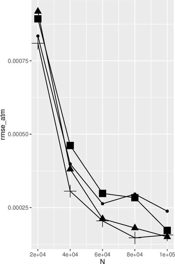
The authors test the method on several derivatives: European calls, Asian options, and variance swaps. They compare against the exact Broadie‑Kaya scheme (adapted by Baldeaux 2012), Andersen’s semi‑explicit scheme, and other popular algorithms. Numerical results show that the proposed method matches or slightly outperforms competitors in terms of root‑mean‑square error and CPU time. The performance improves when model parameters satisfy the Feller condition strongly, as the likelihood correction term becomes small. Sensitivity to the threshold (\delta) is also examined; choosing (\delta) modestly (e.g., (10^{-6})) prevents pathological blow‑up without affecting accuracy.

In conclusion, the paper successfully extends Kouritzin’s explicit weak‑solution technique from the Heston model to the 3/2 model, providing a practically efficient Monte‑Carlo framework for pricing exotic options under a non‑affine volatility dynamics. The approach bridges the gap between exact simulation (which is often computationally heavy) and discretisation‑based schemes (which introduce bias), offering a valuable tool for both researchers and practitioners dealing with 3/2‑type models.