Filling the gaps: Gaussian mixture models from noisy, truncated or incomplete samples

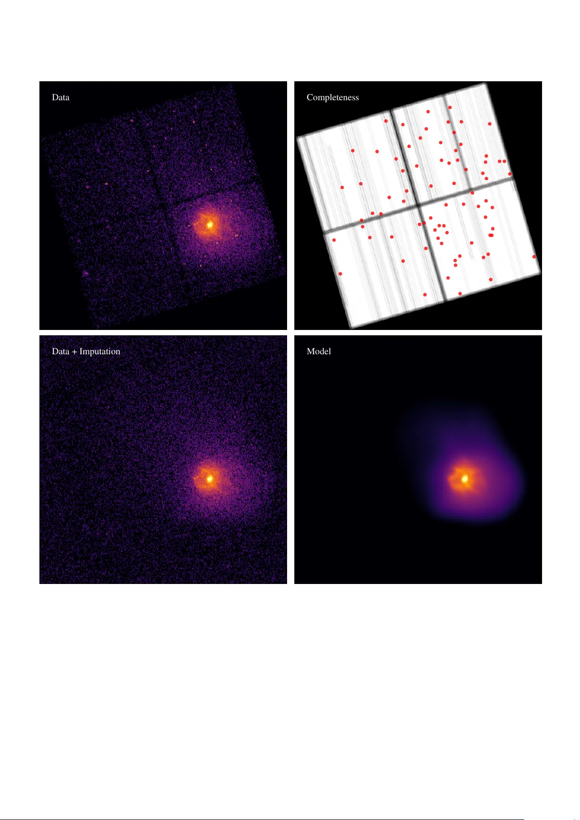
Filling the gaps: Gaussian mixture models from noisy , truncated or incomplete samples Peter Melchior a , Andy D. Goulding a a Department of Astr ophysical Sciences, Princeton University , Princeton, NJ 08544, USA Abstract Astronomical data often su ff er from noise and incompleteness. W e extend the common mixtures-of-Gaussians density estimation approach to account for situations with a known sample incompleteness by simultaneous imputation from the current model. The method, called GMMis , generalizes existing Expectation-Maximization techniques for truncated data to arbitrary truncation geometries and probabilistic rejection processes, as long as the y can be specified and do not depend on the density itself. The method accounts for independent multi v ariate normal measurement errors for each of the observ ed samples and reco vers an estimate of the error-free distrib ution from which both observed and unobserved samples are drawn. It can perform a separation of a mixtures-of- Gaussian signal from a specified background distribution whose amplitude may be unknown. W e compare GMMis to the standard Gaussian mixture model for simple test cases with di ff erent types of incompleteness, and apply it to observational data from the N ASA Chandra X-ray telescope. The python code is released as an open-source package at https://github.com/pmelchior/ pyGMMis . K e ywor ds: density estimation; multiv ariate Gaussian mixture model; truncated data; missing at random 1. Introduction The Gaussian mixture model (GMM) is an important tool for many data analysis tasks, usually employed to approximate a potentially complex density distribution for which there is no suitable parametric form, or to perform a clustering analysis. Its importance is reflected in the wide range of applications and the number of extensions it has received (e.g. McLachlan & Peel , 2000 ; Mengersen et al. , 2011 ). In this work, we will employ the Expectation-Maximization (EM) algorithm to account for “incomplete” samples, i.e. a generalization of truncated sam- ples where data from arbitrarily shaped regions of the feature space hav e a specified probability of not being reported. Also known as “sample selection bias”, it constitutes a long-standing problem for robust inference of population statistics in many scientific disciplines. In observational astronomy , sample incompleteness occurs frequently , caused e.g. by gaps between sensors or by prox- imity to bright objects that render a portion of the observ ation useless. As a milder form of incomplete data, long-running sur- ve ys routinely encounter variations in how well the sky can be observed, for instance when the transparency of the atmosphere or the brightness of the moon changes. As a consequence, sur- ve ys exhibit complicated completeness functions for the density of observed samples and deriv ed data products (e.g. Leistedt et al. , 2016 ). Sev eral approaches for dealing with truncated data within the context of Gaussian mixtures ha ve been presented. Gi ven a simple truncation boundary , one can analytically inte grate the Gaussian density distribution ov er the unobserved regions (e.g. Email addr ess: peter.melchior@princeton.edu (Peter Melchior) W olynetz , 1979 ; Lee & Scott , 2012 , and references therein). McLachlan & Jones ( 1988 ) and Cadez et al. ( 2002 ) developed a method for binned data, which requires integration of the Gaus- sian distribution within bins, and realized that any truncated data can be thought to belong to one extra bin, for which the moments of the GMM are already fully specified by the values in the observed bins. Provided the binning is su ffi ciently fine, this approach allows for arbitrarily shaped truncation bound- aries at the cost of introducing, and integrating ov er , bins for the entire observed re gion. Our approach instead follo ws a proposal by Dempster et al. ( 1977 ) that an estimate of the missing data be drawn from the current model and the EM be run on the combined (observed and estimated missing) data until con ver gence. This approach does not require binning and provides flexibility and compu- tational e ffi ciency . The method we develop here is similar to Multiple Imputation ( Rubin , 1987 ) and Stochastic EM ( Diebolt & Ip , 1996 ) schemes for samples with missing features, and we will draw from the terminology dev eloped in that context to clarify what kind of incompleteness our density-estimation method can account for . While inspired by these earlier works, our contribution enables the treatment of missing samples, not just missing features, an e xtension that renders the GMM ap- plicable to a wide range of observ ational cases. W e also incor- porate the ”Extreme Decon volution” approach of Bovy et al. ( 2011 ) to account for errors of the observed samples and clarify the interplay between noise and missingness. The outline of the paper is as follows: In Section 2 we de- scribe the EM algorithm for GMM optimization, sho w ho w it can accommodate noisy samples, and generalize it for incom- plete and potentially noisy samples. W e discuss sev eral prac- tical extensions of the algorithm in Section 3 and demonstrate Pr eprint submitted to Astr onomy & Computing September 17, 2020 the performance of the proposed algorithm on a variety of test cases in Section 4 . W e present an example application with data from the N ASA Chandra X-ray telescope, exhibiting spatially varying completeness and positional errors, in Section 5 and conclude in Section 6 . The method is implemented in pure python , scalable to mil- lions of samples and thousands of GMM components, and pub- licly released at https://github.com/pmelchior/pyGMMis . 2. GMM from noisy , incomplete samples For a general mixture model o ver a d -dimensional feature space R d , the probability density function (PDF) is p ( x | θ ) = 1 Z ( θ ) K X k = 1 α k p ( x | θ k ), (1) with mixing weights that obey P k α k = 1. The component density functions p ( x | θ k ) with parameters θ k , the list of which { θ 1 , θ 2 , . . . } we simply write as θ , are assumed to be normalized, so that the overall normalization constant Z ( θ ) = 1 and can be dropped. W e will, for the sake of brevity , abbreviate p ( x | θ k ) as p k ( x ). For a GMM, p k is giv en by a multiv ariate normal distribution function, p k ( x ) = N ( x | µ k , Σ k ) ≡ exp  – 1 2 ( x – µ k ) > Σ –1 k ( x – µ k )  p (2 π ) d det( Σ k ) , (2) the complete set of parameters per component is thus α k , µ k , and Σ k . The corresponding mixture log-likelihood for noise- free observ ations D = { x i } with i ∈ { 1, . . . , N } given fixed pa- rameters is ln L ( D | θ ) ≡ N X i ln K X k α k p k ( x i ). (3) This form is also called uncate gorized log-likelihood ( Titter - ington et al. , 1985 ) because there is no information about which component k generated sample i . W e introduce the discrete in- dicator S = ( S 1 , . . . , S N ) with S i = k if (and only if) x i is gener- ated by component k . By rewriting α k p k ( x i ) = q ik p ( x i | α , µ , Σ ) with the conditional probability q ik that x i is generated by com- ponent k , i.e. q ik ≡ Pr( S i = k | x i , α , µ , Σ ), we can form the complete-data log-likelihood p ( x , S | α , µ , Σ ) = p ( x | α , µ , Σ ) + N X i K X k I S i = k ln Pr( S i = k | x i , α , µ , Σ ), (4) the sampling distribution of the complete data ( x , S ) giv en the parameters of the model ( α , µ , Σ ). The second term of the RHS describes the additional information from knowing the alloca- tion S of samples to components ( Fr ¨ uhwirth-Schnatter , 2006 ). 2.1. Standar d EM algorithm As the indicator S is not known or directly observ able, we need to estimate it by classifying each observation. W ith Bayes’ rule, and dropping the conditional dependence on the full set of model parameters ( α , µ , Σ ) in all terms, the classification is giv en by Pr( S i = k | x i ) = Pr( X = x i | S i = k ) Pr( S i = k ) P K j Pr( X = x i | S i = j ) Pr( S i = j ) . (5) W ith it one can re-estimate the parameters of the model from the weighted moments of x giv en the estimate of S . That is the central idea of the EM procedure, which first estimates the classification (the E-step) and then updates the model parame- ters (the M-step). Assuming flat prior distributions Pr( S i = k ) and using the definition of q ik from abov e, we get E-step: q ik ← α k p k ( x i ) P j α j p j ( x i ) M-step: α k ← 1 N X i q ik ≡ 1 N q k µ k ← 1 q k X i q ik x i Σ k ← 1 q k X i q ik h ( µ k – x i )( µ k – x i ) > i . (6) Dempster et al. ( 1977 ), later corrected by W u ( 1983 ), showed that repeated iterations of these tw o steps monotonically con- ver ge to a local maximum of L . 2.2. EM algorithm with noisy samples Observed data often exhibit measurement uncertainties, which we assume to be additiv e and Gaussian: y i ≡ x i + e i , (7) where e i ∼ N ( 0 , S i ). W e want to emphasize that we do not assume that errors are identically distributed, only that they are independent, Gaussian, and that their co variance matrices are known. Bovy et al. ( 2011 ) derived an extended EM algorithm that maximizes the likelihood of the noise-free density p ( x ) from noisy samples y i . The key insight is that one can marginal- ize over the unknown v alues x i and still obtain a GMM. W ith T ik ≡ Σ k + S i the EM procedure amounts to E-step: q ik ← α k p k ( y i | µ k , T ik ) P j α j p j ( y i | µ j , T ij ) b ik ← µ k + Σ k T –1 ik ( y i – µ k ) B ik ← Σ k – Σ k T –1 ik Σ k M-step: α k ← 1 N X i q ik ≡ 1 N q k µ k ← 1 q k X i q ik b ik Σ k ← 1 q k X i q ik h ( µ k – b ik )( µ k – b ik ) > + B ik i , (8) 2 By including measurement uncertainties in the definition of q ik , the M-step is almost unchanged: the role of x i , which is not directly observable, is played by b ik , and the cov ariances get extra contrib utions B ik . All of those modifications vanish when S i → 0 . The resulting EM algorithm still con verges monotoni- cally to a local maximum of L . 2.3. EM algorithm with incomplete samples W e will now account for sample incompleteness, by which we mean the following: the probability of a sample x being observed at all is determined by a completeness function, Ω ( x ) : R d → [0, 1], which means that in any region R ⊂ R d the density of observed samples can systematically deviate from the true density in that region. Formally , p o ( x | θ , Ω ) = 1 Z ( θ , Ω ) Ω ( x ) p ( x | θ ), (9) with Z ( θ , Ω ) ≡ Z d x Ω ( x ) p ( x | θ ). (10) The corresponding log-likelihood is ln L o ( D | θ , Ω ) = N X i ln p o ( x i | θ , Ω ). (11) Such a situation may arise if a measurement de vice is incapable of recording samples from R , so that Ω ( x ) = 0 ∀ x ∈ R . This is the typical situation of truncated samples. A softer version is giv en by Ω ( x ) < 1, which occurs when observ ations su ff er from under-reporting. 1 Before we adapt the EM algorithm to incorporate Ω , it is in- structiv e to clarify how our concept of completeness relates to the terminology of “missingness” introduced by Rubin ( 1976 ) for missing features. In Appendix A we argue that the situa- tion we find here is equiv alent to “missing at random” (MAR), which allows for an arbitrary dependence of Ω on x . This in- cludes Ω ( x ) = const., a case called “missing completely at ran- dom” (MCAR), which is irrele vant for density estimation be- cause it is cancelled from Equation 9 . Thus, MCAR data have the same expectation value of p ( x ) as completely observ ed data, the estimate is merely constrained by fewer samples. On the other hand, the data are not allowed to conform to the most general case called “missing not at random” (MN AR), which would arise from a relation between the missing data and the density itself, Ω ( x ) → Ω ( x , p ( x ) ) (see e.g. Schafer & Gra- ham , 2002 ). A generalization, which cannot use the factoriza- tion p o ( x ) ∝ Ω ( x ) p ( x ) of Equation 9 , goes beyond the scope of this work. As the form of the likelihood function L under MAR is un- changed up to a normalization constant, the E-step remains un- changed as well, and all corrections appear in the M-step. Lee 1 W ithout a loss in generality , we will assume that o ver-reporting has been properly corrected, so that Ω ( x ) ≤ 1, e.g. by Ω ( x ) → Ω ( x )  max x { Ω ( x ) } . W e implicitly assume that there are not false positi ves in the data. & Scott ( 2012 ) demonstrated that the e ff ects of simple trunca- tion of a GMM can be addressed by computing the zeroth, first, and second moments of each Gaussian component when trun- cated in the same way as the data, which requires the analytic integration of p k within the observ ed bounds. Essentially , the update equations for µ k and Σ k get a correction term from the di ff erence between the current-iteration parameters and their truncated values. As we seek the ability to employ arbitrary completeness functions, with complex spatial shapes and prob- abilistic rejection, the analytical integration becomes cumber- some, so we prefer approaches that draw samples from Ω . 2.3.1. Stochastic EM W e adapt the Stochastic EM ( Diebolt & Ip , 1996 ) concept of augmenting missing data features by drawing imputing sam- ples from the current model. In our case, entire samples can be unobserved, as opposed to some of their features being miss- ing. W e thus need apply the selection process described by Ω and keep the rejected samples, i.e. we perform rev erse rejection sampling with the current GMM as the proposal distribution. In detail, we dra w S samples from the GMM and split them into those that we w ould hav e observed O and those that would be missing M . The combined distrib ution has, by construction, the distrib ution Ω ( x ) p ( x ) + ( 1 – Ω ( x ) ) p ( x ) = p ( x ), for which the previous EM equations ( Equation 6 for the noise-free case, and Equation 8 for the noisy case) naturally hold. If we adjust S , so that |O| is consistent with N (the number of actually observed samples in D ), we can replace O with D , and S becomes the current estimate of the number of samples our data set would ha ve had without rejection by Ω . Equation 6 is extended thusly: E-step: q ik ← α k p k ( x i ) P j α j p j ( x i ) ∀ i ∈ {D , M} M-step: α k ← 1 N + |M| X i ∈D q ik + X i ∈M q ik ! ≡ 1 N 0 q k µ k ← 1 q k X i ∈D q ik x i + X i ∈M q ik x i ! Σ k ← 1 q k X i ∈D q ik h ( µ k – x i )( µ k – x i ) > i + X i ∈M q ik h ( µ k – x i )( µ k – x i ) > i ! . (12) Because of the linearity of the equations, the correction terms for the moments can be computed from M missing samples and added to the ones we compute for D . The normalization con- stant Z can be obtained from the imputation sample by Monte Carlo integration, Z ( θ , Ω ) ≈ 1 S X x ∈{D , M} Ω ( x ), (13) of which only the contrib ution from M has to be determined in each iteration. In case of a binary Ω , Z ≈ N S . 3 This approach, which we will call GMMis , in which at each iteration we draw and augment the observed data with imputa- tion samples, is summarized in Algorithm 1 . It is guaranteed to maximize the complete-data log-likelihood and conv erges to a stationary distribution for the parameters ( α , µ , Σ ) ( Diebolt & Ip , 1996 ; Nielsen , 2000 ). T o the best of our knowledge, this is the first time that a GMM approach has been made robust against not just truncation but the generalized form of incom- plete sampling. This method is e ffi cient where p ( x ) ( 1 – Ω ( x ) ) is large; cor- rection for weakly expressed components are more di ffi cult to attain because M is dra wn globally from the entire GMM, as opposed to being drawn from each component individually . A minor limitation is that when Ω is lar ge for a component, the values of the M -sums in the M-step equations are not well de- termined, howe ver their impact on the result is also minor be- cause that component is mostly observed. In comparison with an analytic ev aluation of the PDF in the unobserved re gions, this approach is fle xible and e ffi cient, does not require numerical integrations of the component distribu- tions, b ut, due to its stochastic nature, su ff ers from sample vari- ance in the correction terms because M has finite size. As with all Stochastic EM approaches, it generates sequences of L o that are not guaranteed to monotonically increase in every step . T o reduce the stochastic contribution to L o , we can average the correction terms from M ov er multiple draws of size S , so that the corrections become more precise and L o -sequences closer to monotonic. W e found that a veraging over ≈ 10 imputation samples results in sample variances that are small compared to the increase of the observed likelihood. 2.3.2. Incompleteness and Noise Besides speed and flexibility , GMMis retains the ability to deal with noisy samples. By adding noise to the imputation samples M , we can e valuate q ik , b ik , and B ik for i ∈ M and modify Equation 8 analogously to Equation 12 : E-step: q ik ← α k p k ( y i | µ k , T ik ) P j α j p j ( y i | µ j , T ij ) ∀ i ∈ {D , M} b ik ← µ k + Σ k T –1 ik ( y i – µ k ) ∀ i ∈ {D , M} B ik ← Σ k – Σ k T –1 ik Σ k ∀ i ∈ {D , M} M-step: α k ← 1 N + |M| X i ∈D q ik + X i ∈M q ik ! ≡ 1 N 0 q k µ k ← 1 q k X i ∈D q ik b ik + X i ∈M q ik b ik ! Σ k ← 1 q k X i ∈D q ik h ( µ k – b ik )( µ k – b ik ) > i + X i ∈M q ik h ( µ k – b ik )( µ k – b ik ) > i ! . (14) As before, the corrections from M hav e the same form as, and are added to, the moments calculated for D . But to do so, we hav e to define T ik = Σ k + S i for the missing samples, which Algorithm 1 GMMis A GMM is fit to observed samples D = { x i } i = 1, ... , N , accounting for a specified sample completeness Ω by drawing imputation samples M from the current-iteration GMM and accepting those with a rate 1 – Ω . For noisy observations with covariances { S i } , GMMis requires an error model S ( x ) for the entire data region. 1: procedur e GMMis ( { x i } , Ω ( x ), tol, [ { S i } , S ( x ) ] ) 2: for t = 1, 2, . . . do 3: Z t ← { z i ∼ p ( x | α t , µ t , Σ t ) } i = 1, ... , S t 4: R t ← { r i ∼ U (0, 1) } i = 1, ... , S t 5: M t ← { z i : r i < 1 – Ω ( z i ) } i = 1, ... , S t 6: if S t – |M t |  Poisson( N ) then 7: S t ← S t ( S t – |M t | ) / N 8: go to Line 3 9: if { x i } noise-free then 10: q t + 1 ← Equation 12 (E-step) 11: α t + 1 , µ t + 1 , Σ t + 1 ← Equation 12 (M-step) 12: else 13: S t z ← { S ( z i ) } z i ∈M it 14: M t ← { z 0 i ∼ N ( z i , S t z i ) } z i ∈M it 15: q t + 1 , b t + 1 , B t + 1 ← Equation 14 (E-step) 16: α t + 1 , µ t + 1 , Σ t + 1 ← Equation 14 (M-step) 17: ln L t + 1 o ← Equation 11 & Equation 13 18: if | ln L t + 1 o – ln L t o | < tol · ln L t o then break which we lack observed uncertainties. These uncertainties may be known ev en in unobserved regions. If not, we need to make a guess of S ( x ) in the unobserved re gion, e.g. from the mean or a smooth interpolator of the observed S i . W e must stress that not assuming errors for M would result in it having too large a weight in the likelihood. In the E-step, samples from M w ould be e valuated without noise, while the observed samples hav e a broadened likelihood under noise. As a result, the EM algorithm would become dominated by miss- ing samples and yield density estimates that are unduly shifted tow ards regions of low Ω . On the other hand, we do not hav e to exactly match the uncertainties of M to those of D because they only enter as sums in the M-step. Matching the average errors of the samples associated with each component, instead of each indi vidual sample, is therefore su ffi cient to estimate the parameters of all components. W e finally note that adding noise and applying Ω do not commute; in either order , GMMis requires only that M can be created such that it completes the data with an estimate of the unobserved portion. 3. Practical considerations 3.1. Initialization The EM algorithm only guarantees con vergence to a local maximum of the likelihood. W ith the large number of free pa- rameters of the GMM (1 + d + d ( d + 1) / 2 for each of K com- ponents), a suitable initialization is critical. Several initializa- tion schemes hav e been proposed (e.g. Biernacki et al. , 2003 ; 4 Bl ¨ omer & Bujna , 2013 ). For a completely observed data set, we adopt the simplest strategy , namely drawing the means at ran- dom from the data. In detail, giv en a user-defined length scale s , for each component k we draw i at random from { 1, . . . , N } and ∆ x i ∼ N ( ~ 0, s 2 I ), and set α k = 1 / K µ k = x i + ∆ x i Σ k = s 2 I , (15) which naturally follows the distribution of the data on scales larger than s . T o prev ent strong initial localization, s should be chosen to exceed the typical clustering scale of the data, but small enough that multiple components do not strongly o verlap. In the case of incomplete samples, we initially mak e the as- sumption that it was complete, i.e. Ω = 1, fit a GMM to the observed distribution, and use that fit to initialize the run with a specified Ω , 1. While this approach will obviously fail if a component is entirely located in a region with Ω = 0, we found that an initial guess based on the observed distribution much more quickly con ver ges than the random initialization de- scribed above. T o aid the exploration of the regions with Ω < 1, we leav e the components means unchanged b ut multiply the co- variances by a factor > 1. If that factor is chosen too small, the EM algorithm will not be able to pick up the correction terms P i ∈M q ik etc. in Equation 12 before re-con ver ging to the pre vi- ous, observed-sample location. In turn, if the factor is chosen too large, the con vergence is slo wed do wn. W e therefore rec- ommend a factor of 2 – 4, i.e. increasing the linear size of each component by 50 – 100%, as a compromise that works well in practice. 3.2. Split-and-mer ge operations W ith a large number of free parameters, the EM algorithm can easily get trapped in local maxima of L . For clustered data, this beha vior leads to GMM components being placed across sev eral clusters or a single cluster being shared by multiple components. In the latter case, the weight α k tends to zero for at least one of those components. T o improv e the performance of the GMM, Ueda et al. ( 2000 ) devised criteria to decide whether a component should be merged with another or be split into two. Performing both of these op- erations at the same time amounts to altering three distinct com- ponents with the total number of components being conserved. W e follo w this approach, with two alterations we found to per- form better for all cases with d = 2, 3 we inv estigated. Ueda et al. ( 2000 ) proposed to merge the components k and l that maximize J merge ( k , l ) = Q > k Q l , (16) with Q > k = ( q 1 k , . . . , q Nk ), i.e. the components whose posterior cluster assignment p ( k | x ) are most similar across the entire data set. This works well in practice as long as there are no “empty” components, which do unfortunately arise in multi- modal situations if more components are locally av ailable than are needed to explain the data. Because q ik → 0 when α k → 0, the merge criterion abo ve will not seek to merge such empty components even though they are obviously excellent choices to be mer ged. W e therefore replace Q k → Q k  α k , which means that we seek to merge components whose p k ( x ) is most similar for the entire data set. For the split criterion, we found that the one suggested by Ueda et al. ( 2000 ), based on the Kullback-Leibler div ergence, is unduly a ff ected by outliers and often leads to split candi- dates that do not improve the lik elihood. Instead, we took guid- ance from a proposal of Zhang et al. ( 2003 ) on how to best re-initialize the two new components that result from a split, namely to separate their means along the semi-major axis of the ellipsoid described by the pre-split Σ . W ith this intuition it is natural to identify split candidates according to their largest eigen value λ 1 of Σ . When searching for the component k = argmax k { λ k ,1 } , we assume it is strongly elongated because it seeks to describe two clusters at once. The main failure mode of that split criterion is again related to (almost) empty compo- nents. Their parameters, in particular Σ k , are only poorly deter - mined. Some of them are erroneously large and would thus be identified as split candidates, while they constitute much better merge candidates. W e thus propose to identify split candidates by selecting k as the one that maximizes J split ( k ) = α k λ k ,1 . (17) While the original split criterion of Ueda et al. ( 2000 ) will seek to eliminate any de viation of the local density from its approx- imation by a Gaussian-shaped component and is therefore gen- erally applicable, our criterion appears to perform better for identifying a prominent failure mode for unconstrained GMMs: components that merge two clusters. As the split is only ac- cepted if it leads to an overall increase in the likelihood, it does not lead to increased fragmentation from penalizing the largest components. Following Zhang et al. ( 2003 ), we then replace the means of two newly split components l and m as µ l , m = µ k ± 1 2 EV 1 ( Σ k ), i.e. along the primary eigenv ector of the cov ariance matrix. When dealing with incomplete data, we hav e not found split- and-merge operations to be problematic. They are most useful when enabled during the initialization run as described in Sec- tion 3.1 , which will then not be plagued by strong f ailure modes of the EM algorithm. As a result, the imputation samples M will be more reliable, and the full algorithm will conv erge faster than without split-and-merge operations. 3.3. Minimum covariance re gularization One problem of the objective function L is that it becomes unbounded if µ k = y i for any k and i because Σ k → 0 . Bovy et al. ( 2011 ) presented a regularization scheme to set a lower bound for every component v olume. In its simplest version it assumes the form of a d -dimensional sphere with variance w , which modifies the last update equation in Equation 8 according to Σ k ← 1 q k + 1         X i q ik h ( µ k – b ik )( µ k – b ik ) > + B ik i + w I         . (18) 5 In principle, the value of w is entirely arbitrary , but we choose to provide a more intuitive setting and associate it with a mini- mum scale ω in feature space, below which the model does not possess explanatory power , i.e. we want det( Σ k ) ≥ ω 2 d . For a constant regularization term, we need to adopt a typical value of q k , for which we use its mean over all components, ¯ q k = N K . W e can thus set w = ω 2 ( N K + 1). This choice does not provide an exact lower bound for each component as we determine the regularization term from the av erage value of q k , which leads to stronger regularization for components with small α k . W e con- sider this an advantage in noisy situations, where the parameters of weakly expressed components can be hard to determine. W e note, howe ver , that the form of the regularization in Equation 18 prefers features in the data to be of approximately equal size, otherwise the penalty term can dominate for small features while being ine ff ectiv e for large features. 3.4. F itting for a backgr ound distrib ution In many situations, observed data comprise anomalous sam- ples that appear unclustered, i.e. unrelated to the features of in- terest, and rather originate from a more uniform “background” distribution. One solution within the context of GMMs would be to add another component with very large v ariance and to fit for its amplitude only . W e prefer to introduce a specific back- ground distribution ov er the relev ant region R of feature space, e.g. the most con ventional form of a uniform background p bg ( x ) =        h R R d x i –1 = const. x ∈ R 0 x < R . (19) If the amplitude of the background component ν is unknown, one can introduce a two-le vel mixture model for the combined density distribution (e.g. Fr ¨ uhwirth-Schnatter , 2006 , their sec- tion 7.2.4), p ( x | α , µ , Σ , ν ) = (1 – ν ) K X k = 1 α k p k ( x ) + ν p bg ( x ), (20) but we prefer k eeping the model strictly linear in the amplitudes and put the component and background amplitudes on equal footing: p ( x | α , µ , Σ , ν ) = K X k = 1 α k p k ( x ) + ν p bg ( x ). (21) In this form, P k α k = 1 – ν . T o determine the amplitude ν we require another indicator variable q i bg to denote if a sample x i belongs to the background. Analogous to q ik in Equation 6 it is giv en by the posterior of x i under the background model, which leads to these E-step equations q ik ← α k p k ( x i ) P k α k p k ( x i ) + ν p bg ( x i ) q i bg ← ν p bg ( x i ) P k α k p k ( x i ) + ν p bg ( x i ) . (22) The M-step for the background amplitude is ν ← 1 N X i q i bg , (23) while the M-step of the GMM components remains unchanged. If the samples are noisy , the previous equations in this sec- tion hold, but we need to marginalize ov er the positions of the unobserved noise-free samples ( Bovy et al. , 2011 ) and modify the background distribution as p bg ( y i | S i ) = Z d x p bg ( x ) N ( y i | x , S i ), (24) which is equi valent to the change to the GMM q ik in Equation 8 compared to the noise-free case in Equation 6 . For the uniform background distribution the marginalization amounts to the ze- roth moment of the truncated multi variate normal distribution (e.g. Manjunath & W ilhelm , 2012 ). One could think that sample incompleteness does not a ff ect the inference of the background component because any infor- mation how Ω ( x ) acts on samples drawn from p bg is already entirely contained in Ω ( x ) itself. 2 The problem with this notion is that we do not know the relative amplitudes of signal and background in the unobserved re gions, which will vary because the signal does. For consistent results, we therefore create the imputation sample M by drawing from the GMM and the back- ground model according to the current-iteration v alue of ν , and proceed as in Section 2.3 . W e caution that the introduction of a background compo- nent leads to additional uncertainties and a higher-dimensional parameter space. In particular , during the first iterations of the EM algorithm, the parameters of the GMM often only provide rather poor description of the data, so that many samples will hav e higher probability under the background model, resulting in few samples left to fit for the GMM parameters in the ne xt iteration. This failure mode highlights the importance of a suit- able initialization when working with a background model, es- pecially when its intensity becomes dominant. T o this end, we found in our tests that the k -means initialization from Bl ¨ omer & Bujna ( 2013 , their Algorithm 1) performed more robustly than the random initialization of Equation 15 . 3.5. A veraging estimators Even with well-chosen initial values and split-and-merge operations, any single GMM will get trapped in local maxima of the likelihood. W e therefore advocate, for two reasons, to av erage sev eral GMMs fit to the same data, a technique also known as ensemble learning. First, ensemble estimators typically outperform ev en the best single estimator . In particular, Smyth & W olpert ( 1999 ) built an improved estimator by employing the “stacking” method proposed by W olpert ( 1992 ), which uses the cross-validation re- sult to determine non-negati ve weights for each model (see also 2 The presence of a non-vanishing background intensity can therefore in principle be used to estimate Ω ( x ). Howev er , for this work we require Ω to be known a priori. 6 Breiman , 1996 ). In the context of GMMs, it is useful to realize that a mixture of mixture models is still a mixture model, there- fore no conceptual changes have to be made when ev aluating the estimator . Second, stacked GMMs reduce the need to determine the optimal number of components K . The main concern when de- termining K is that if set too high, the resulting GMM overfits the data, following spurious features that increase the variance in the prediction, while if set too low , the model does not cap- ture essential features of the data, leading to a large prediction bias. As this topic has been extensiv ely discussed else where, we will not address it here. W e do note, howe ver , that stacking exhibits better trade-o ff s between bias and variance than single- model selection or uniform averaging, rendering stacked GMM particularly robust against ov erfitting ( Smyth & W olpert , 1999 ). Even more so, combining GMMs with di ff erent K , or di ff erent cov ariance constraints, can provide a natural framew ork to de- scribe data with a variety of spatial scales. A decision if and how single-run GMMs are to be av eraged will depend on the characteristics of the data at hand. In this work, we will only use single-run results to allow the reader to ev aluate the performance of GMMis rather than that of the av eraging scheme. 4. Experiments 4.1. A toy e xample W e first perform a simple test with no model misspecifica- tion, i.e. we draw the original sample from a GMM with K = 3. In Figure 1 , we show that sample as red circles. W e then add a noticeable amount of Gaussian noise (blue contours) and im- pose a purely geometric completeness Ω ( x ), whose boundaries are given by a box and a circle (dotted curves), resulting in the test sample (blue squares). W ith this test case we demonstrate how the EM algorithm reacts to noise and a non-trivial com- pleteness. The standard EM algorithm (top-center panel) does what one needed to expect, namely to describe the observed sample as is. It clearly prefers the region inside of the bound- aries and thereby misestimates amplitudes, locations, and co- variances of the components a ff ected by Ω . W ith the noise-decon volution approach of Bovy et al. ( 2011 ), summarized in Equation 8 , one can attempt to recov er the noise- free distribution. Howe ver , in this case (shown in the top-right panel of Figure 1 the resulting shrinkage of the components is detrimental to the overall likelihood because the model is now ev en more confined to the observed region, reducing its abil- ity to also describe samples beyond that. In essence, the model is biased as before but more confident in its correctness as the noise contribution has been remov ed. W e generically find it to be true that noticeable incompleteness will need to be ad- dressed first, and only then can one properly deconv olve from the noise, as we demonstrate with the progressi ve impro vement in the next two tests. When the sample incompleteness from Ω is correctly spec- ified and considered via Equation 12 , GMMis recov ers compo- nent centers, orientations, and amplitudes much better (bottom- left panel), howe ver the cov ariances remain inflated as the pres- ence of noise is not yet corrected for . This lev el of model fidelity could have been achieved with analytical integration ( W olynetz , 1979 ; Lee & Scott , 2012 ) or sample binning ( McLach- lan & Jones , 1988 ; Cadez et al. , 2002 ), but here none of those operations were necessary . In addition, neither of the aforemen- tioned approaches can account for incompleteness and noise. In the bottom-center panel, we use the full algorithm, i.e. the noise decon volution of Equation 8 applied to both the O and M samples in Equation 12 , resulting in the highest lik elihood of the three v ariants, with just ∆ ln L = –0.151 compared to red sample drawn from the true underlying PDF . By running the full algorithm (with Ω and noise treatment) ten times, we can inv estigate the spread associated with the giv en data set under the admittedly restrictiv e assumption of a GMM with K = 3. The bottom-right panel of Figure 1 , whose contours have the same stretch as those of the previous pan- els, sho ws that there are considerable di ff erences between runs, mostly associated with the Ω -boundaries. Also, the compo- nents from di ff erent runs emphasize the importance of di ff er- ent apparent sub-clusters. This behavior is caused by the added noise, which obscures the presence of small-scale features. As we attempt to infer the noise-free PDF from noisy samples, the models will amplify small-scale density fluctuations. Because of such spurious sub-clusters or, more generally , local minima of the likelihood, we advocate the use of more sophisticated av eraging schemes, as outlined in Section 3.5 . 4.2. Limits of applicability W e want to inv estigate, in a more di ffi cult, highly multi- modal situation, how strongly incomplete the sampling can be for the proposed method to still yield reasonable density esti- mates. W e therefore set up a new test case in which we place K = 50 GMM components randomly in the d = 3 unit cube. Cov ariances are chosen such that the overlap between the com- ponents is not excessi ve; weights are drawn from a symmetric Dirichlet distribution with concentration parameter of unity . W e impose a probabilistic completeness function p ( Ω | x ) = 1 – x 1 , i.e. a linear ramp from fully observed to fully missing along one of the coordinate axes. The purpose of this setup is to allow all combinations of component weight α k and completeness Ω . W e draw N = 10,000 samples from the model, apply Ω , and record the size of samples N k drawn from each component k as well as the mean Ω k experienced by those samples, so that we kno w the observed sample size N O k = N k Ω k . No noise is added to the samples. An example cube is sho wn in Figure 2 . W e then fit the test data with another GMM with the same K = 50, resulting in best-fit parameters ˜ θ , and repeat the pro- cess 10 times. As diagnostic, we directly compare the densities ρ ( x ) by splitting the cube into 50 3 cells and counting the input samples that fall into the cell covering x . W e do the same for the predicted density ˜ ρ ( x ) by dra wing N samples from the fit. As we kno w the expectation value of Ω at the location of each cell, we can compute the fractional bias in the predicted density  ˜ ρ ( x ) – ρ ( x )  ρ ( x ) as a function of Ω ( Figure 3 ). The standard EM algorithm pro vides a reliable estimate of the observed den- sity , in other words: the bias is equal to Ω . The reason for 7 T ruth log L = –3.962 σ Standard EM log L = –4.676 Standard EM & noise decon v olution log L = –4.967 GMMis log L = –4.232 GMMis & noise decon v olution log L = –4.113 Dispersion Figure 1: T est case for the EM algorithm with noisy and incomplete samples. T op left : True density distribution (contours in arcsinh stretch), a deri ved sample with N = 400 (red open circles, whose av erage log L under the respective models is giv en in the top-left corner of each panel), and the test sample (blue squares) after adding Gaussian noise (whose 1,2,3 σ contours are sho wn in the bottom-right corner) and rejecting all points outside of the box or inside the circle (dashed curves). T op center : Result of the standard EM algorithm ( Equation 6 ). T op right : Result of the standard EM algorithm with noise decon volution ( Equation 8 ). Bottom left : Result of the proposed EM algorithm GMMis ( Equation 12 ), assuming noise-free samples. Bottom center : Result of GMMis , accounting the noise of the O and M samples. Bottom right : Standard de viation of the predicted p ( x ) from 10 runs of GMMis as in the bottom-center panel. Markers, if present, and completeness boundaries are identical in all plots. positiv e bias for Ω > 1 2 lies in the normalization of the density estimator: as we drew the same number of samples N from the model as where giv en as input data, any underestimation of the density must be compensated elsewhere. In the same test, GMMis shows a noticeably reduced sensi- tivity to Ω , b ut the resulting density estimate is still biased. This test demonstrates that there must be conditions under which the proposed algorithm fails. It is obvious that we cannot expect GMMis , or any other density estimator, to infer the properties or ev en existence of a cluster that is entirely unobserved, i.e. N O k = 0. Even for less extreme cases, Figure 3 shows that GMMis struggles with samples from regions with low Ω , over - compensating where Ω is large. T o determine limits of applicability , we e valuate how well the input samples from each component are described by the fit. W e compute the association fraction η k of the input sam- ple from component k that falls within “1 σ ” of any compo- nent of the fit, which, for d > 1, is more precisely expressed as { i : ( x i – ˜ µ k ) > ˜ Σ k ( x i – ˜ µ k ) ≤ χ 2 d (0.683) for any k } , where χ 2 d is the quantile function of the chi-squared distribution with d degrees of freedom. For a component of the test data whose samples are perfectly fit (i.e. fit by the component from which they are generated), the association fraction should on average be η k = 68.3%. If η k is higher , either the associated component of the fit is too extended or the test samples are associated with multiple components. If η k is lower , the fit has e ff ectively ig- nored some samples from input component k . In Figure 4 we plot η k as a function of the e ff ectiv e weight N O k  N O of com- ponent k giv en the observed data, while the size of the marker encodes the initial weight α k = N k  N , and the color encodes Ω k . It is apparent that components of the test data with lar ge α k or Ω k are generally well-described by the fit. For Ω k ≈ 0, the fit will miss a large fraction of the original sample irrespective of α k , but there are also a few well-observed b ut low- α compo- nents that are largely being ignored by the fit. There is also an increased tendency of fitting multiple nearby input clusters with one lar ger component, which leads to artificially lar ge η k at lo w N O k  N O . W ithout formal proof, we seek a criterion to identify components that are too poorly observed to yield a reasonable fit. By performing the test described above with di ff erent val- 8 0.0 0.2 0.4 0.6 0.8 1.0 0.0 0.2 0.4 0.6 0.8 1.0 0.0 0.2 0.4 0.6 0.8 1.0 Figure 2: Example test data generated from K = 50 clusters in the d = 3 unit cube. The completeness Ω is probabilistic, decreasing linearly from unity (left side of the cube) to zero (right side). Observed samples are shown in blue, missing samples in red. ues of N , K , component volumes, and Dirichlet concentration parameter , we found N O k N O = N k Ω k P k N k Ω k ' 1 K (25) to perform well (shown as vertical dotted line in Figure 4 ). This qualitativ ely agrees with findings of e.g. Naim & Gildea ( 2012 ) that the best GMM fits with an EM algorithm are achieved when all components hav e approximately equal weights, in particular when they ov erlap. It also implies that GMMis has to success- fully fit the observed distribution first to be able to generate meaningful imputation samples M that account and correct for Ω . If the first step is flawed, the second one will be, too. This two-step picture is confirmed when we remov e from the test data all components that would have violated Equa- tion 25 , in other words, the test data now only comprises clus- ters that remain salient despite Ω . In this case, the algorithm can detect all present clusters and correct for the sample incom- pleteness. Accordingly , the GMMis density estimates are now largely unbiased (dash-dotted red line in Figure 3 ). W e empha- size that this shortcoming is not caused by an incorrect form of the likelihood, rather by the economy of the EM algorithm to con verge to the nearest likelihood maximum, which fa vors the most prominent clusters in the observed sample. If, on the other hand, the parameters of all but one component were fixed at their true v alues and there were only one component left to fit, this component could experience incompleteness in excess of Equation 25 and still be fit with a fidelity commensurate to its number of samples N k . 5. Application to Chandra X-ray data T o demonstrate the capabilities of GMMis , we analyze the distribution of X-ray photons of the nearby galaxy NGC 4636, 0.0 0.2 0.4 0.6 0.8 1.0 Ω –1.0 –0.5 0.0 0.5 1.0 ( ˜ ρ – ρ )/ ρ uncorrected Ω perfect correction Standard EM GMMis GMMis , N o k / N o > 1/ K Figure 3: Relative bias of the density estimator as function of completeness Ω . The density is calculated by generating N = 10, 000 samples from the fit and binning them into 50 3 cells within the unit cube: for the standard EM algorithm (blue) which does not correct for incomplete samples; for GMMis (solid red); for GMMis after removing all poorly observed components from the input data that do not obey Equation 25 (red dash-dotted). observed with the Advanced CCD Imaging Spectrometer (A CIS) aboard the Chandra telescope. These data were retrieved from the Chandr a public archi ve, and consist of two individual 75 ks pointings (Observation Identification Numbers 3926 and 4415). Basic data processing was carried out following the procedure described in Goulding et al. ( 2016 ). Briefly , we used the Chan- dra X-ray Center pipeline software packages available in ciao v4.7 to apply the latest detector calibration files, and remov e the standard pix el randomization, streak events, bad pixels, and cosmic rays. Photon catalogs (referred to as “ev ents files”) were screened using a typical grade set (grade = 0, 2, 3, 4, 6), and cleaned of 3 σ background flares. Finally , aspect histograms were constructed and con volved with the A CIS-I chip map, us- ing the cia o tool mkexpmap , to generate the observation specific exposure time maps. In the top-left panel of Figure 5 we show a histogram of ≈ 150,000 photons in the energy range E ∼ 0.5 – 2 keV , covering an area with a side-length of about 0.3 degrees. T wo features of the observation are obvious. First, there are small gaps be- tween the four CCDs of ACIS-I, where the ability to record photons is strongly reduced. In detail, A CIS additionally suf- fers from minor and well-kno wn sensiti vity de gradations in dif- ferent parts of the CCD (top-right panel of Figure 5 ). Second, besides the galaxy , there is an essentially uniform particle back- ground, as well as additional smaller objects (“point sources”). These point sources are a mixture of X-ray binary systems that are intrinsic to NGC 4636 and distant, rapidly growing super- massiv e black holes unrelated to the tar get g alaxy . W e mask the point sources with small circular apertures (shown as red dots), a step that is commonly done in the analysis of X-ray data. As a further complication, the photon positions are not known exactly as the y hav e been con volved with the instrument Point- spread function (PSF), which for this ACIS-I has a shape that 9 0.00 0.02 0.04 0.06 0.08 0.10 N o k / N o 0.0 0.2 0.4 0.6 0.8 1.0 η k 1 σ re gion 1/ K 0.0 0.2 0.4 0.6 0.8 1.0 Ω k Figure 4: Associated fraction η k of input samples to fit components as function of the e ff ective weight in the observed data. Marker sizes denote weights α k in the input data, colors refers to the av erage completeness Ω k experienced by input components k . Both N O k and Ω k are known exactly from the test setup. The horizontal dashed line shows the perfect outcome of 68.3% of the samples found within the “1 σ region” of an output component; the vertical dashed line shows the criterion Equation 25 for lik ely unrecoverable components. is very well approximated by a circular Gaussian 3 with a width that varies from 0.4 arcsec in the inner region of A CIS-I to 15 arcsec at the perimeter . Our new method is ideally suited to directly analyze the photon ev ent files. W e can account for chip gaps, field edges, sensitivity variations, and point-source masks with the basic GMMis algorithm from Section 2.3 . By recognizing that con- volution with the PSF is formally identical to additiv e mea- surement noise, we can employ the decon volution method from Section 2.2 to build a generative model of the underlying, noise- free distribution of X-ray photons, while simultaneously fitting for the X-ray background as described in Section 3.4 . In con- trast, a more traditional image analysis typically entails smooth- ing, which does not correctly account for an y form of sample incompleteness, and a single deconv olution step, which does not incorporate the spatial variation of the PSF width. The bottom-left panel of Figure 5 demonstrates the princi- ple of operations. By drawing samples from the current state of the model, which comprised the GMM and the uniform back- ground, conv olving them with the spatially varying PSF , and selecting them according to Ω , we get a sample to augment the observed data. Combining this imputation sample and the point-source masked data, we get a representation of the in- ternal state of the model, in other words: its estimate how the data would look like if Ω = 1. In each iteration these aug- mented data enter Equation 14 to determine the best-fit model of the extended emission of the galaxy without point sources (bottom-right panel). W e initialize the GMM with K = 60 components with means distributed according to a biv ariate Gaussian, whose width s 3 See the Chandra Proposers’ Observatory Guide, http://cxc.harvard. edu/proposer/POG/ was determined by fitting the galaxy with K = 1 first. Be- cause the scene exhibits features of di ff erent scales, we set the component cov ariances to Σ k = 4 – l s 2 I with l = 0, . . . , 5, and 10 components at each lev el l . This tailored initialization is necessary despite the GMM’ s ability to adjust to arbitrary con- figurations because the rate of conv ergence is very slo w for the weakly expressed features we are particularly interested in. The background amplitude ν was allowed to vary between 0.2 and 0.5, with ν = 0.396 being the best-fit value, in other words about 40% of the photons over the unobscured region shown in Figure 5 originate from the background. The GMM is capable of faithfully describing large and small- scale features in the data: a bright, apparently bimodal central region, most likely arising due to the presence of an accret- ing supermassiv e black hole; an extended halo of low-intensity emission from di ff use, 10 5 – 10 7 Kelvin hot gas with a notice- able ske wness tow ards the lower right corner; and the location and intensity of se veral shock fronts caused by b uoyantly ris- ing pockets of plasma that were likely inflated during previous outbursts of the central supermassiv e black hole. Ho wev er , be- cause of the complexity of the model with K = 60, it is not guaranteed that particular features, e.g. shock fronts, are fit by a single component. This association could be made more clear if the analysis operated on a three-dimensional feature space of photon positions and energies, a study we lea ve for the future. Because this is a demonstration of the capabilities of the method, we hav e not performed e.g. cross-validation tests to determine the optimal K . The model is the result of a single run with a number of components that appeared visually reasonable to capture the key features of the data. Its χ 2 per degree of freedom over an area where the galaxy dominates the emission is at least 1.34, 4 indicating that a larger number of components may be necessary to capture all significant features. 6. Summary and conclusions W e describe a novel extension of the EM algorithm to per- form density estimation with Gaussian mixture models in situ- ations where the data exhibits a known incompleteness Ω . The type of incompleteness may be described by a sharp boundary , a case that is usually denoted as “truncated data”, or by an arbi- trary probabilistic function Ω ( x ), as long as the mechanism that causes the incompleteness is independent of the density ( miss- ing at r andom ). The ke y di ff erence of the method described here to the situ- ation that is often—and some what ambiguously—called “miss- ing data” is that the latter refers to data, for which some features of an y data sample may be absent. In contrast, we deal with en- tire samples being potentially absent, caused by the systematic limitation to observe the entire feature space or all of its relev ant regions. 4 For the estimate of the degrees of freedom we assumed that no parameters are learned from the data, yielding an upper bound on the dof. If all parameters were linearly independent, which is not an appropriate assumption for GMMs, the dof would be reduced by 3%. 10 Data Completeness Data + Imputation Model Figure 5: Application to X-ray data. T op left : Histogram of the locations of photons in the ener gy range 0.5–2 keV for an observation of the galaxy NGC 4636 with the A CIS-I instrument of the Chandra X-ray telescope. T op right : Completeness Ω ( x ) for A CIS-I, determined by the location of its four CCDs and detector sensitivity variations; point source masks (red circles, sizes true to scale), where we reject data and explicitly set Ω = 0, ha ve been added for the purpose of this analysis. Bottom left : ACIS-I data augmented with the imputation sample drawn from the final models of the GMM and the background. Bottom right : Final GMM with K = 60 of the extended emission of the galaxy , after rejecting point sources, removing the background, and recon volving to match the observ ation. The images are aligned such that North is up and East is left; all panels are shown in logarithmic stretch. Our solution is based on drawing imputation samples from the current state of the GMM, and to recompute the model pa- rameters in the M-step using both observed and missing sam- ples. This technique is applicable to any generative model that is fit with an EM algorithm, as demonstrated with the signal– background model of Section 3.4 . Its advantage is the flexi- bility to e ffi ciently adjust to any incompleteness Ω ( x ) because one a voids the analytic integration of the predicted density o ver the incomplete regions. Instead, we draw test samples from the current model, retain those that would not have been observed under Ω , and obtain non-zero contributions to the moments of those components that extend into incompletely observed re- 11 gions. If the model is suitable to describe the data-generating process, adding those moments to the ones obtained from the observed samples results in parameter estimates consistent with those for completely observed data. W e detail practical refinements of the algorithm, regard- ing its initialization, split-and-merge operations, and simulta- neously fitting for a uniform background. W e also recommend av eraging GMMs from independent runs to smooth out the de- pendence of the EM algorithm on the starting position to esti- mate the uncertainty of the estimators. In simplified tests we demonstrate that the algorithm 1. recov ers an estimate of the underlying density in pres- ence of complex incompleteness functions, 2. correctly accounts for incompleteness and additiv e noise if the imputation samples describe the noisy unobserved data, 3. can only partially correct for incompleteness if the too many of the original samples ha ve not been observ ed. The last finding is central to the applicability of the method. Constraining complex GMMs with finite amounts of samples becomes even more challenging with non-neglibible incomplete- ness. Correcting for the latter requires being able to perform the former reasonably well, otherwise the imputation samples do not describe the true unobserved samples. In absence of an analytical estimate of the fidelity of GMMs from the EM al- gorithm, we provide a best-e ff ort estimate for the limits of the algorithm in Equation 25 . W e demonstrate the usefulness of the algorithm with exam- ple data from the NASA X-ray telescope Chandra , where the incompleteness stems from g aps between the chips of the A CIS instrument. W e directly estimate the extended emission of the galaxy NGC 4636 from the location of photon hits, while ac- counting for the window-frame configuration of the detector; a spatially varying point-spread function; and a uniform X-ray background. The presented method provides an e ffi cient and flexible tool to estimate the density of a process that is a ff ected by moder - ate lev els of incompleteness of the MAR type. As such situa- tions may arise in many areas of the physical and social sci- ences, we believ e this contribution to be of general use and hav e therefore made our python implementation av ailable at https://github.com/pmelchior/pyGMMis . Appendix A. Missingness for density estimation T o understand what form the likelihood assumes when some samples are not observed, we need to determine how observed and missing samples are related. For this purpose Rubin ( 1976 ) introduced the missingness mechanism R that determines which part of the complete data Y is observed ( Y o ) or missing ( Y m ). The relation between R and Y o or Y m giv es rise to three distinct types of missingness: p ( R | Y ) =              p ( R ) missing completely at random (MCAR) p ( R | Y o ) missing at random (MAR) p ( R | Y o , Y m ) missing not at random (MN AR) Under MCAR, the missingness mechanism does not depend on the data at all; in turn, the data do not rev eal properties of R . The key distinction between MAR and MNAR is whether R depends only on observed or also on missing features. For the problem of density estimation with incomplete sam- ples x , it is not immediately obvious what Y o and Y m corre- spond to. W e take guidance from the close relation between density estimation and function approximation by positive lin- ear operators (e.g. Ciesielsky , 1991 ). W e therefore take X to be the entire feature space R d and Y = R the co-domain of a scalar function p : X → Y , namely the PDF p ( x ). The data then span ( X , Y ) = R d + 1 , and R determines at what locations x a value y ∈ Y is recorded. In Section 2.3 , we introduced the completeness function Ω ( · ), which is equiv alent to p ( R | · ). Only a spatially uniform completeness function fulfills the MCAR condition, but is irrel- ev ant for density estimation as the resulting probability density function is simply a renormalized version of the true PDF . If Ω only depends on x , the MAR condition applies because X is by construction completely observed (only values of Y may be missing). T echnically , MAR still holds if Ω depends on x and the density p ( x 0 ) at some other observed position x 0 , x , for instance when the observed samples “shadow” some oth- ers. F or the sake of brevity , we have not listed this case in Section 2.3 . Only if samples are missing because of their own value of y = p ( x ), or because of their relation to other miss- ing values p ( x 0 ), we hav e MN AR. This can happen e.g. when an experimental de vice is locally in validated by saturation or if samples are only recorded if their local abundance exceeds a certain threshold. An in vestigation under which conditions the proposed approach can account for MN AR cases is beyond the scope of this paper . References Biernacki C., Celeux G., Gov aert G., 2003, Comput. Stat. Data Anal. , 41, 561 Bl ¨ omer J., Bujna K., 2013, preprint, () Bovy J., Hogg D. W ., Ro weis S. T ., 2011, Annals of Applied Statistics , 5, 1657 Breiman L., 1996, Machine Learning , 24, 49 Cadez I. V ., Smyth P ., McLachlan G. J., McLaren C. E., 2002, Mach. Learn. , 47, 7 Ciesielsky Z., 1991, Probability And Mathematic Statistics, 12, 1 Dempster A. P ., Laird N. M., Rubin D. B., 1977, Journal of the Royal Statistical Society . Series B (Methodological), 39, 1 Diebolt J., Ip E., 1996, in W .R. Gilks S. Richardson D. S., ed., , Markov Chain Monte Carlo in Practice. Chapman & Hall, London Fr ¨ uhwirth-Schnatter S., 2006, Finite Mixture and Markov Switching Models. Springer Series in Statistics, Springer New Y ork, http://www.springer. com/us/book/9780387329093 Goulding A. D., et al., 2016, ApJ , 826, 167 Lee G., Scott C., 2012, Comput. Stat. Data Anal. , 56, 2816 Leistedt B., et al., 2016, ApJS , 226, 24 Manjunath B. G., W ilhelm S., 2012, preprint, () McLachlan G. J., Jones P . N., 1988, Biometrics , 44, 571 McLachlan G., Peel D., 2000, Finite Mixture Models, Wile y Series in Prob- ability and Statistics. John W iley & Sons, New Y ork, https://books. google.com/books?id=YXqflwEACAAJ Mengersen K. L., Robert C., Titterington M., 2011, Mixtures: estimation and applications. V ol. 896, John Wile y & Sons Naim I., Gildea D., 2012, preprint, () Nielsen S. F ., 2000, Bernoulli , 6, 457 Rubin D. B., 1976, Biometrika , 63, 581 12 Rubin D., 1987, Multiple Imputation for Nonresponse in Surv eys, W iley Se- ries in Probability and Statistics. W iley Series in Probability and Statistics, W iley , https://books.google.com/books?id=0KruAAAAMAAJ Schafer J. L., Graham J. W ., 2002, Psychological Methods , 7, 147 Smyth P ., W olpert D., 1999, Machine Learning , 36, 59 T itterington D., Smith A., Makov U., 1985, Statistical analysis of finite mix- ture distributions. Wile y series in probability and mathematical statistics: Applied probability and statistics, Wile y , https://books.google.com/ books?id=hZ0QAQAAIAAJ Ueda N., Nakano R., Ghahramani Z., Hinton G. E., 2000, Journal of VLSI signal processing systems for signal, image and video technology , 26, 133 W olpert D. H., 1992, Neural Netw . , 5, 241 W olynetz M. S., 1979, Journal of the Royal Statistical Society . Series C (Ap- plied Statistics), 28, 195 W u C. F . J., 1983, The Annals of Statistics, 11, 95 Zhang Z., Chen C., Sun J., Chan K. L., 2003, Pattern Recognition , 36, 1973 13