Sub-linear Memory Sketches for Near Neighbor Search on Streaming Data

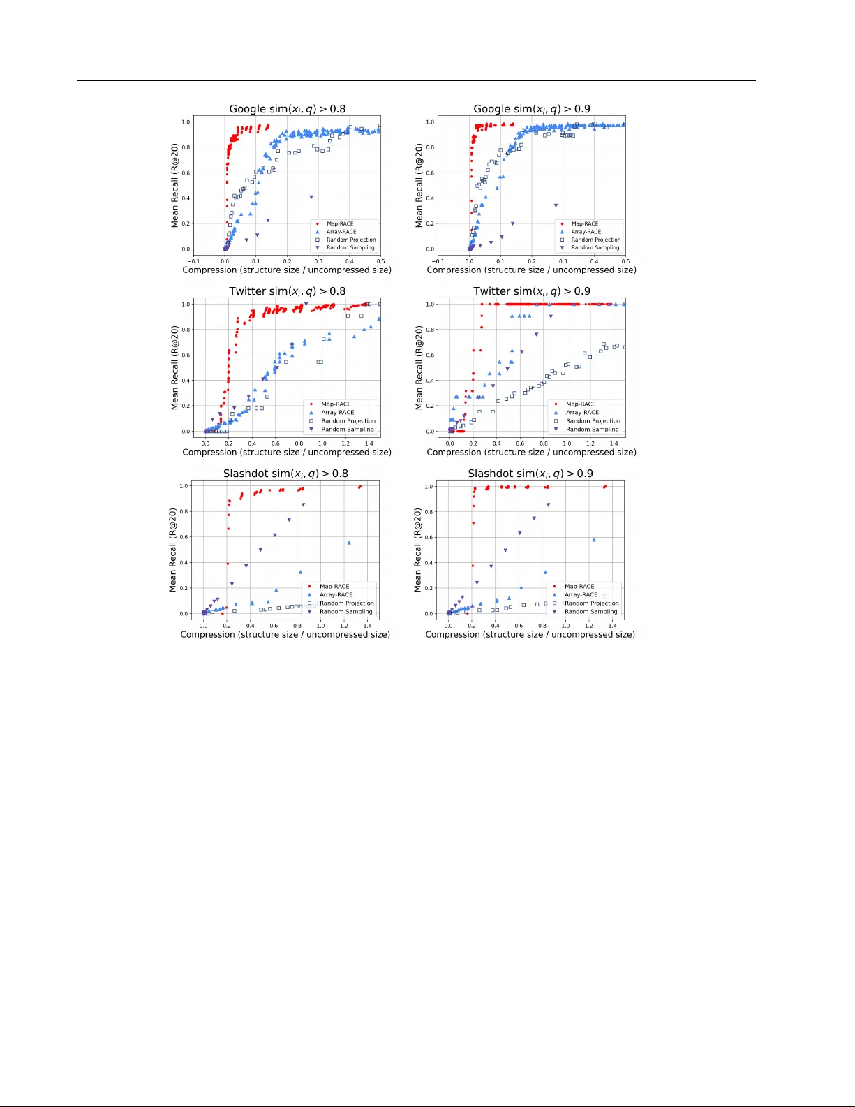
Sub-linear Memory Sketches f or Near Neighbor Sear ch on Streaming Data Benjamin Coleman 1 Richard G Baraniuk 1 2 Anshumali Shrivasta va 1 2 Abstract W e present the first sublinear memory sketch that can be queried to find the nearest neighbors in a dataset. Our online sketching algorithm com- presses an N element dataset to a sketch of size O ( N b log 3 N ) in O ( N ( b +1) log 3 N ) time, where b < 1 . This sketch can correctly report the near- est neighbors of any query that satisfies a sta- bility condition parameterized by b . W e achiev e sublinear memory performance on stable queries by combining recent advances in locality sensi- tiv e hash (LSH)-based estimators, online kernel density estimation, and compressed sensing. Our theoretical results shed ne w light on the memory- accuracy tradeoff for nearest neighbor search, and our sketch, which consists entirely of short integer arrays, has a v ariety of attractive features in practice. W e ev aluate the memory-recall trade- off of our method on a friend recommendation task in the Google Plus social media network. W e obtain orders of magnitude better compres- sion than the random projection based alternativ e while retaining the ability to report the nearest neighbors of practical queries. 1. Introduction Approximate near-neighbor search (ANNS) is a funda- mental problem with widespread applications in databases, learning, computer vision, and much more (Gionis et al., 1999). Furthermore, ANNS is the first stage of se veral data processing and machine learning pipelines and is a popular baseline data analysis method. Informally , the problem is as follows. Giv en a dataset D = x 1 , x 2 , ..., x N , observed in a one pass sequence, b uild a data structure S that can ef- ficiently identify a small number of data points x i ∈ D that 1 Department of Electrical and Computer Engineering, Rice Univ ersity , Houston, T exas, USA 2 Department of Computer Sci- ence, Rice University , Houston, T exas, USA. Correspondence to: Benjamin Coleman < ben.coleman@rice.edu > , Anshumali Shri- vasta va < anshumali@rice.edu > . Pr oceedings of the 37 th International Confer ence on Machine Learning , Online, PMLR 119, 2020. Copyright 2020 by the au- thor(s). hav e high similarity to any dynamically generated query q . In this paper , we focus on low-memory ANNS in settings where it is prohibitive to store the complete data in any form. Such restrictions naturally arise in extremely large databases, computer networks, and internet-of-things sys- tems (Johnson et al., 2019). W e want to compress the dataset D into a sketch S that is as small as possible while still retaining the ability to find near-neighbors for any query . Furthermore, the algorithm should be one pass as the second pass is prohibiti ve when we cannot store the full data in any form. It is common wisdom that the size of S must scale linearly ( ≥ Ω( N ) ), even if we allo w algorithms that only identify the locations of the nearest neighbors. In this work, we challenge that wisdom by constructing a sketch of size O ( N b log 3 N ) bits in O ( N b +1 log 3 N ) time. Our sketch can identify near-neighbors for stable queries with high probability in O ( N b +1 log 3 N ) time. The value of b depends on the dataset, but b can be significantly less than 1 for many applications of practical importance. It should be noted that our sketch does not return the near neighbors themselves, since we do not store the vectors in any form. Instead, we output the identity or the index of the nearest neighbor , which is sufficient for most appli- cations and does not fundamentally change the problem. Our sketch also does not attempt to correctly answer ev- ery possible near-neighbor query in sublinear memory , as this would violate information theoretic lower bounds. In- stead, we provide a graceful tradeof f between the stability of a near neighbor search query and the memory required to obtain a correct answer . 1.1. Our Contribution Our main contribution is a one-pass algorithm that pro- duces a sketch S that solves the exact v -nearest neighbor problem in sub-linear memory with high probability . A for- mal problem statement is av ailable in Section 2.3 and our theoretical results are formally stated in Section 4. Our al- gorithm requires O ( N b +1 log 3 N ) time to construct S and the same time to return the v nearest neighbors for a query . Here, b is a query-dependent v alue that describes the stabil- ity or difficulty of the query . Our guarantees are general and work for any query , but the sketch is only sub-linear when b < 1 . In practice, one commits to a giv en b value and obtains the guarantees for all queries satisfying our condi- Sub-linear Memory Sketches f or Near Neighbor Search on Streaming Data tions. W e obtain our sketch by merging compressed sensing tech- niques with recently-developed sketching algorithms. Sur- prisingly , we find that the hardness of a near-neighbor query is directly related to the notion of sparsity , or signal- to-noise ratio (SNR), in compressed sensing (Donoho, 2006; Tropp & Gilbert, 2007). This connection allows us to analyze geometric structure in the dataset using the v ery well-studied compressed sensing framework. The idea of exploiting structure to improve theoretical guarantees has recently gained traction because it can lead to stronger guarantees. For instance, the first improvements over the seminal near-neighbor search results of (Indyk & Motwani, 1998) were obtained using data-dependent hashing (An- doni et al., 2014). These methods use information about the data distrib ution to generate an optimal hash for a gi ven dataset. In this work, we assume that the dataset has a set of general properties that are common in practice and we con- struct a data structure that e xploits these properties. In gen- eral, the communication complexity of the near neighbor problem is O ( N ) . Our method requires sub-linear memory because our data assumptions limit the set of valid queries. W e support our theoretical findings with real experiments on large social-network datasets. Our theoretical tech- niques are sufficiently general to accommodate a variety of compressed sensing methods and KDE approximation algorithms. Howe ver , in practice we apply our theory us- ing the Count-Min Sketch (CMS) as the compressed sens- ing method and the recently-proposed RACE sketch for KDE (Coleman & Shri vasta va, 2020). Our RA CE-CMS sketch inherits a variety of desirable practical properties from the RA CE and CMS sketches that are used in its con- struction. When implemented this way , our near neighbor sketch consists entirely of a set of integer arrays. Further- more, RACE sketches are linear , parallel and mergeable, allowing us to realize many practical gains using RACE- CMS. For instance, despite a query time comple xity that is theoretically worse than linear search, RACE-CMS can be implemented in such a way that it is fast and practical to construct and query , processing thousands of vectors each second. As a result, we belie ve that our method will enable a v ariety of practical applications that need to perform near neighbor search in the distributed streaming setting with limited memory . 2. A pplications Here, we describe se veral applications for low-memory near neighbor sketches. Graph Compression for Recommendation: In recom- mendation systems, we represent relationships, such as friendship or co-purchases, as graphs. Gi ven N users, we represent each user as an N dimensional sparse vector , where non-zero entries correspond to edges or connections. T o perform recommendations, we often wish to find pairs of users that are mutually connected to a similar set of other users. The process of identifying these users is a similarity search problem ov er the N dimensional sparse vector rep- resentation of the graph (Hsu et al., 2006). Online graphs can be very large, with billions of nodes and trillions of edges (Ching et al., 2015). Since graphs at this scale are prohibitiv ely expensi ve to store and transmit, methods ca- pable of compressing the netw ork into a small and informa- tiv e sketch could be inv aluable for large-scale recommen- dations. Robust Caching: The process of caching previously- seen data is a central component of many latency-critical applications including search engines, computer networks, web browsers and databases. While there are many well- established methods, such as Bloom filters, to detect ex- act matches, caching systems cannot currently report the distance between a query element and the contents of the cache. Our sketches can be used to implement caching mechanisms that are robust to minor perturbations in the query . Such a capability naturally provides better anomaly detection, robust estimation and retriev al. Since similar data structures can fit into the cache of modern proces- sors (Luo & Shriv astav a, 2018), our sketches could be an effecti ve practical tool for online caching algorithms. Distributed Data Streaming: In application domains such as the internet-of-things (IoT) and computer networks, we often with to build classifiers and other machine learn- ing systems in the streaming setting (Ma et al., 2009). In practice, sketching is a critical component of distributed data collection pipelines. For instance, Apple uses a wide variety of sketches to enable mobile users to transmit valu- able information that can be used to train machine learning models while minimizing the data transmission cost (Apple Differential Pri vacy T eam, 2017). Similar challenges occur with distributed databases and IoT settings, where data gen- erators can be scattered across a network of connected de- vices. Such applications require sketching methods to min- imize the data communication cost while preserving utility for downstream learning applications. Since our sketches consist of integer arrays, they can easily be serialized and sent ov er a network. 2.1. Related W ork The problem of finding near-neighbors in sub-linear time is a very well-studied problem with sev eral solutions (In- dyk & Motwani, 1998). Howe ver , the memory r equirement for near-neighbor search has only recently started receiv- ing attention (Indyk & W agner, 2018; 2017). Although hueristic methods for sample compression are employed in Sub-linear Memory Sketches f or Near Neighbor Search on Streaming Data T able 1: Summary of related work. Results are shown for a d -dimensional dataset of N points. Existing methods (Johnson & Lindenstrauss, 1984; Indyk & W agner, 2018; Agarwal et al., 2005) can estimate distances to all points in the dataset with a 1 ±  multiplicati ve error (full  dependence not shown). Our method estimates the similarity with all points ha ving a ±  additi ve error , where b depends on the properties of the dataset. Method Sketch Size (bits) Sketch T ime Comments No compression dN log N N/A - Random projections (Johnson & Lindenstrauss, 1984) N log 2 N N log N W idely used in practice Compressed clustering tree (Indyk & W agner, 2018) N log N N d log O (1) N Multiple passes Coresets (Agarwal et al., 2005) d − ( d − 1) N +  − ( d − 1) Multiple Passes This work N b log 3 N N b +1 log 3 N b < 1 for stable queries practice, the best theoretical result in this direction requires O ( N log N ) memory and therefore does not break the lin- ear memory bound (Indyk & W agner, 2018). T able 1 con- tains a summary of e xisting work in the area. T o the best of our knowledge, the algorithm described in this paper is the first to perform near-neighbor search using asymptotically sub-linear memory . Coresets or Clustering Based Appr oaches: A reason- able compression approach is to construct a coreset or rep- resent the dataset as a set of clusters. For instance, the widely-used F AISS system compresses vectors using prod- uct quantization (Jegou et al., 2010). There are also sam- pling procedures to construct a subset P of D and guaran- tee the existence of a point p ∈ P such that d ( p, x ) <  for  > 0 . The cluster-based approach from (Har-Peled & Kumar, 2014) uses similar ideas to reduce the space for v -nearest-neighbor by a constant factor of 1 v . Ho w- ev er , our procedure is superior in the follo wing two regards. First, coresets and sample-based compression methods re- quire parallel access to the entire dataset at once to deter- mine which points to retain in the sketch. As an example, the sketch in (Har-Peled & Kumar, 2014) requires an of- fline clustering step. Therefore, it is impossible to stream queries to the sketch efficiently using existing methods. Second, cluster approximations of the data cannot solve the exact v -nearest neighbor problem because the sketch- ing process removes points from the dataset. Despite the guarantees that can be obtained using  coverings of the dataset, there may be any number of near -neighbors within  of the query that ha ve been discarded during sketching. Perhaps most importantly , our method requires weaker as- sumptions about the dataset. Cluster -based methods as- sume that the dataset has a clustered structure that can be approximated by a small collection of centroids. T o achiev e high compression ratios, coreset methods require similar assumptions. Howe ver , our method is valid ev en when there is no efficient cluster representation. Our weak assumptions are particularly applicable to recent problems in recommendation systems, graph compression and neural embedding models. In this context, we are given a dataset where each embedding or object representation is close to a relatively small number of other elements. Furthermore, we expect most of our queries to be issued in regions that contain only a few elements from the dataset. Although there may be no large-scale hierchical clustering structure, our method can exploit the weaker structure in the dataset to pro vide good compression without the need for complex clustering and sample compression algorithms. Finally , we note that our approach is much simpler to un- derstand and analyze than e xisting methods. While cluster - ing methods can achiev e good performance, they usually require complex distance-approximation methods at query time. Sketch construction consists of computationally- intensiv e clustering steps or coreset sampling routines that hav e many moving parts. In contrast, our data structure is a simple array of integer counters with a fixed size. There- fore, we expect that our method will be attracti ve to practi- tioners and system designers. 2.2. Background Our algorithm uses recent advances in locality-sensitiv e hashing (LSH)-based sketching with standard compressed sensing techniques. Before covering our method in detail and presenting theoretical results, we briefly revie w some useful results in sketching and compressed sensing. 2.3. Problem Statement In this paper, we solve the exact v -nearest neighbor prob- lem. The v -nearest neighbor problem is to identify all of the v closest points to a query with high probability . The difficulty of the v -nearest neighbor problem is data- dependent. T o capture the dif ficulty of a query , we use the notion of near-neighbor stability from the seminal pa- per (Beyer et al., 1999). Definition 1. Exact v -near est neighbor Given a set D of points in a d -dimensional space and a Sub-linear Memory Sketches f or Near Neighbor Search on Streaming Data parameter v , construct a data structure which, given any query point q , r eports a set of v points in D with the fol- lowing pr operty: Each of the v near est neighbors to q is in the set with pr obability 1 − δ . Definition 2. Unstable near-neighbor sear ch A near est neighbor query is unstable for a given  if the distance fr om the query point to most data points is ≤ (1 +  ) times the distance fr om the query point to its nearest neighbor . 2.4. Compressed Sensing and the Count Min Sk etch Compressed sensing is the area in signal processing that deals with the reco very of compressible signals from a sub- linear number of measurements. The task is to recover an N -length vector x from a vector y of M linear combina- tions, or measurements, of the N components of x . The problem is tractable when x is v -sparse and has only v nonzero elements. F or a more detailed description of the compressed sensing problem, see (Baraniuk, 2007). The fundamental result in compressed sensing is that we can exactly recover x from y using only M = O ( v log N /v ) measurements. In the streaming literature, the v nonzero elements are of- ten called heavy hitters . The Count-Min Sketch (CMS) is a classical data summary to identify heavy hitters in a data stream. The CMS is a d × w array of counts that are in- dex ed and incremented in a randomized fashion. Giv en a vector s , for ev ery element s i in s , we apply d univ er- sal hash functions h 1 ( · ) , ...h d ( · ) to i to obtain a set of d indices. Then, we increment the CMS cells at these in- dices. When all elements of s are non-negati ve, we ha ve a point-wise bound on the estimated s i values returned by the CMS (Cormode & Muthukrishnan, 2005). For the sake of simplicity , we only consider the CMS when presenting our results. Finding heavy hitters is equiv alent to compressed sensing (Indyk, 2013), and there are an enormous number of valid measurement matrices in the literature (Candes & Plan, 2011). Other compressed sensing methods can im- prov e our bounds, b ut we defer this discussion the supple- mentary materials. Theorem 1. Given a CMS sketch of the non-negative vec- tor s ∈ R N + with d = O  log  N δ  r ows and w = O  1   columns, we can r ecover a vector s CMS such that we have the following point-wise r ecovery guar antee with pr obabil- ity 1 − δ for each r ecover ed element s CMS i : s i ≤ s CMS i ≤ s i +  | s | 1 (1) 2.5. Locality-Sensitive Hashing LSH (Indyk & Motwani, 1998) is a popular technique for efficient approximate nearest-neighbor search. An LSH family is a f amily of functions with the following property: Under the hash mapping, similar points have a high proba- bility of having the same hash value. W e say that a collision occurs whenev er the hash values for two points are equal, i.e. h ( p ) = h ( q ) . The probability Pr H [ h ( p ) = h ( q )] is known as the collision probability of p and q . In this pa- per we will use the notation p ( p, q ) to denote the collision probability of p and q . For our ar guments, we will assume a slightly stronger notion of LSH than the one giv en by (In- dyk & Motwani, 1998). W e will suppose that the colli- sion probability is a monotonic function of the similarity between p and q . That is p ( p, q ) ∝ f (sim( p, q )) (2) where sim( p, q ) is a similarity function and f ( · ) is mono- tone increasing. LSH is a very well-studied topic with a number of well-kno wn LSH families in the literature (Gio- nis et al., 1999). Most LSH families satisfy this assump- tion. 2.6. Repeated Array-of-Counts Estimator (RA CE) Recent work has shown that LSH can be used for effi- cient unbiased statistical estimation (Spring & Shri vasta va, 2017; Charikar & Siminelakis, 2017; Luo & Shriv astav a, 2018). The RA CE algorithm (Coleman & Shriv astav a, 2020) replaces the uni versal hash function in the CMS with an LSH function. The result is a sketch that approximates the kernel density estimate (KDE) of a query . Here, we re-state the main theorem from (Luo & Shri vastav a, 2018) using simpler notation. Theorem 2. ACE Estimator (Luo & Shrivastava, 2018) Given a dataset D , an LSH function l ( · ) 7→ [1 , R ] and a parameter K , construct an LSH function h ( · ) 7→ [1 , R K ] by concatenating K independent l ( · ) hashes. Let A ∈ R R K be an array of O ( R K log N ) bits wher e the i th component is A [ i ] = X x ∈D 1 { h ( x )= i } Then for any query q , E [ A [ h ( q )]] = X x ∈D p ( x, q ) K W e will heavily leverage the observation that A [ h ( q )] is an unbiased estimator of the summation of collision prob- abilities. This sum is a kernel density estimate over the dataset (Coleman & Shriv astav a, 2020), where the kernel is defined by the LSH function. Sub-linear Memory Sketches f or Near Neighbor Search on Streaming Data Algorithm 1 One-Pass Online Sketching Algorithm Require: D Ensure: d × w RA CE arrays indexed as A i,j,o Initialize: k × d × w × R independent LSH family (denoted by L ( · ) ) and d independent 2-universal hash functions h i ( · ) , i ∈ [1 − d ] , each taking v alues in range [1 − w ] . while not at end of data D do read current x j ; for o in 1 to r do for i in 1 to d do A i,h i ( j ) ,o [ L [ x j ]] ++; end for end for end while Algorithm 2 Querying Algorithm Require: Sketch from Algorithm 1, query q Ensure: Identities of T op- v neighbors of q W e already hav e: k × d × w × R independent LSH family (denoted by L ( · ) ) and d independent 2-uni versal hash functions h i ( · ) , i ∈ [1 − d ] , each taking values in range [1 − w ] from Algorithm 1. for i in 1 to d do for j in 1 to w do CMS ^ ( i,j ) = MoM ( A i,j,o [ L ( q )]) end for end for for j in 1 to n do s ^ j = p ^ ( q , x j ) K = min i CMS ^ ( i,h i ( j )) end for Report top- v indices of s ^ as the neighbors. 3. Intuition W e propose Algorithm 1 as an online near -neighbor sketch- ing method and Algorithm 2 to query the sketch. The intu- ition behind our algorithm is as follo ws. Consider the nai ve method to perform near-neighbor search. W e begin by find- ing the pairwise distances between the query and each point in the dataset. Given a query q , this procedure results in a vector of N distances, where the i th position in the vector contains the distance d ( x i , q ) . If j is the index of the small- est element in the vector , then x j is the nearest neighbor to the query . Now suppose that we are giv en a vector s of N kernel ev aluations rather than explicit distances. Here, the i th component of s is s i = k ( x i , q ) , where k ( · , · ) is a radial kernel. Radial kernels are nearly 1 when d ( x i , q ) is small and decrease to 0 as d ( x i , q ) increases. Since k ( x i , q ) is a monotone decreasing function with respect to d ( x i , q ) , the vector of kernel values is also sufficient to perform near neighbor search. If s j is the largest component of s , then x j is the nearest neighbor to the query . The main idea of our algorithm is to apply compressed sensing techniques to s . The main result from compressed sensing is that a sparse vector s can be recovered from a sub-linear memory sketch of its components. If we assume that s is v -sparse (contains only v elements that are large), then we can recover s from O ( v log N /v ) random linear combinations of the entries of s . The key insight is that each measurement is a weighted kernel density estimate (KDE) over the dataset. Using a small collection of KDE sums, we can identify the near neighbors of the query . If we choose the coef ficients to be { 1 , 0 } , then each measurement is an unweighted KDE o ver a partition of the dataset. While it requires N memory to compute the exact KDE, recent results (Coleman & Shri- vasta va, 2020) show that the KDE may be approximated by an online sketch in space that is constant with respect to N . While larger sketches improve the quality of the ap- proximation, the memory does not gro w when elements are added to the dataset. Thus, each of the O ( v log N/v ) mea- surements can be approximated using constant memory in the streaming setting. 4. Theory Due to space constraints, we omit proofs and corner cases. For a thorough presentation that includes proofs, see the supplementary material. 4.1. Estimation of Compressed Sensing Measur ements T o bound the error of the approximation for our com- pressed sensing measurements, we bound the variance of the RA CE estimator using standard inequalities. Theorem 3. Given a dataset D , K independent LSH func- tions l ( · ) and any choice of constants r i ∈ R , RACE can estimate a linear combination of s i ( q ) = p ( x i , q ) K with the following variance bound. E [ A [ L ( q )]] = X x i ∈D r i p ( x i , q ) K (3) v ar( A [ l ( q )]) ≤ | ˜ s ( q ) | 2 1 (4) wher e L ( · ) is formed by concatenating the K copies of l ( · ) and ˜ s i ( q ) = p s i ( q ) . Let y ∈ R M be the M compressed sensing measurements of the KDE vector s ( q ) . A direct corollary of Theorem 3 is that by setting the coefficients correctly , we can obtain un- biased estimators of each measurement with bounded v ari- ance. Using the median-of-means (MoM) technique, we can obtain an arbitrarily close estimate of each compressed sensing measurement. T o ensure that all M measurements obey this bound with probability 1 − δ , we also apply the Sub-linear Memory Sketches f or Near Neighbor Search on Streaming Data probability union bound. Note that the multiplicativ e M factor comes from the fact that we are using A CE to esti- mate M different measurements. Theorem 4. Given any  > 0 and O  M | ˜ s ( q ) | 2 1  2 log  M δ  independent ACE repetitions, for any query q , we have the following bound for each of the M measurements with pr obability 1 − δ y i ( q ) −  ≤ ˆ y i ( q ) ≤ y i ( q ) +  (5) Therefore, by repeating A CE estimators (RA CE), we can obtain low-v ariance estimates of the compressed sensing measurements of s ( q ) . The exact number of measurements M depends on both Φ and the dataset, b ut M < O ( N ) . 4.2. Query-Dependent Sparsity Conditions For our compressed sensing measurements to be useful, s ( q ) needs to be sparse with a bound on | s ( q ) | 1 (Donoho, 2006). W e also require a bound on | ˜ s ( q ) | 1 to av oid a mem- ory blow-up in Theorem 4. If we simply assume a bound on | ˜ s ( q ) | 1 , it is straightforward to show that the sketch re- quires sub-linear memory . See the supplementary materials for details. T o characterize the type of queries that are ap- propriate for our algorithm, we connect sparsity with the idea of near -neighbor stability (Beyer et al., 1999), a well- established notion of query difficulty . Giv en any vector s ( q ) with elements between 0 and 1, we can tune K to make s ( q ) sparse and obtain the required bounds. Ho wever , increasing K also increases the mem- ory because we require increasingly more precise estimates to differentiate between s v and s v +1 . Therefore, we want K to be just large enough. The largest value of K is re- quired when all points in the dataset other than the v near- est neighbors are equidistant to the query ( | s | 1 = O ( N ) ). T o choose K appropriately , we begin by defining tw o data- dependent values ∆ and B to characterize this situation. Suppose that x v and x v +1 are the v th and ( v + 1) th nearest neighbors, respecti vely . Let ∆ be defined as ∆ = p ( x v +1 ,q ) p ( x v ,q ) and B = P N i = v +1 ˜ s i ˜ s v +1 . ∆ measures the stability (Defini- tion 2) of the query and is a measure of the gap between the near-neighbors and the rest of the dataset. If ∆ ≈ 1 , then x v and x v +1 are very dif ficult to separate and the query is unstable . B measures the sparsity of s . If B is O ( N ) , then ev ery element of s is nonzero (Figure 1). W e are now ready to present our results for K in terms of B and ∆ . Theorem 5. Given a query q and query-dependent pa- rameters B and ∆ , if K = l 2 log B log 1 ∆ m then p ( x v , q ) K ≥ P N i = v +1 p ( x i , q ) K and we have the bounds | s ( q ) | 1 ≤ v + 1 and | ˜ s ( q ) | 1 ≤ v + 1 In practice, this assumption is unrealistically pessimistic because s ( q ) is often sufficiently sparse without any inter - vention using K . Ho wever , Theorem 5 always allows us to choose K so that | s ( q ) | 1 is bounded by a constant. 4.3. Reduce Near -Neighbor to Compressed Recovery W e can apply Theorem 4 to estimate each of the M CMS measurements, which we call [ CMS . W e want to recover an estimate ˆ s of s from our approximate compressed sens- ing measurements [ CMS . Since the error  E in our approx- imation simply adds to the CMS recovery error  C from Theorem 1, we can recover the values of s ( q ) by choosing appropriate values for  C and  E . Theorem 6. W e requir e O  | ˜ s ( q ) | 2 1 | s ( q ) | 1  3 log  | s ( q ) | 1 δ log  N δ  log  N δ  A CE estimates to r ecover ˆ s ( q ) with probability 1 − δ such that s i ( q ) −  2 ≤ ˆ s i ( q ) ≤ s i ( q ) +  2 (6) If s is sparse, then this result can be used to identify the top v elements of s by setting  = s v − s v +1 = p K v − p K v +1 . These elements correspond to the largest kernel ev aluations and therefore the nearest neighbors. For the equidistant case, we substitute the value of K from Theorem 5 into the expression in Theorem 6 to obtain our final results. Our main theorem is a simplified result that relates the size of the RA CE sketch with the query-dependent parameters ∆ and p v . The full deriv ation, including the dependence on δ , is av ailable in the supplementary materials. Theorem 7. It is possible to construct a sketch that solves the exact v -near est neighbor pr oblem with pr obability 1 − δ using O  N b log 3 ( N )  bits, wher e b = 6 | log p v | +2 log r log 1 ∆ Her e, r is the range of the LSH function, and p v is the colli- sion pr obability of the v th near est neighbor with the query . 5. Experiments In this section, we rigorously ev aluate our RACE-CMS sketch on friend recommendation tasks on social network graphs, similar to the ones described in (Sharma et al., 2017). Our goal is to compare and contrast the practical compression-accuracy tradeoff of RA CE with streaming baselines. W e use the Google Plus social network dataset, obtained from (Leskovec & Mcauley, 2012), and the T wit- ter and Slashdot graphs from (Leskov ec & Kre vl, 2014) to ev aluate our algorithm. Google Plus is a directed graph of 107,614 Google Plus users, where each element in the dataset is an adjacency list of connections to other users. Sub-linear Memory Sketches f or Near Neighbor Search on Streaming Data Figure 1: Geometric interpretation of B and ∆ . ∆ characterizes the gap between the v nearest neighbors, while B characterizes whether s is sparse. The worst-case situation occurs when all points are equidistant to the query (center). Howe ver , if s is already sparse, then far fe wer points in the dataset are near the query (right). Figure 2: Implementation of sketching (Algorithm 1) and querying (Algorithm 2) using RACE data structures. During sketching, we compute d × w × R × k hash values for each x ∈ D and update the RACEs selected using h ( · ) . During querying, we compute the hash values of the query q and estimate the CMS measurements. T able 2: Dataset Statistics Dataset Nodes Nonzeros Mean Edges Mean Similarity Google+ 108k 13.6M 127 0.002 T witter 81.4k 1.8M 22 2.2e-4 Slashdot 82.2k 1.1M 13 1.4e-5 The uncompressed dataset size is 121 MB when stored in a sparse format as the smallest possible unsigned integral type. The other datasets are structured the same way , with similar sizes. Additional statistics are displayed in T able 2. These characteristics are typical for large scale graphs, where the data is high dimensional and sparse. Note that the low mean similarity between elements indirectly im- plies that s ( q ) is sparse. 5.1. Implementation W e use the RA CE-CMS sketch that was presented in Sec- tion 4. Howe ver , we slightly deviate from the algorithm described in Algorithm 1 in our implementation by rehash- ing the K LSH hash values to a range r using a universal hash function. Our algorithm is characterized by the hyper- parameters K , d, w, R and r and by the hash functions l ( · ) and h ( · ) . Here, l ( · ) is MinHash, an LSH function for the Jaccard distance. W e use MurmurHash for h ( · ) , the uni- versal hash function in the CMS. For all experiments, we vary K , d, w and R to trade off memory for performance. W e present the operating points on the Pareto frontier for all algorithms. T ypical v alues of d are between 2 and 5, w between 100 and 1000, and R between 2 and 8. W e varied the range r between 100 and 1000 and used K ∈ { 1 , 2 } . W e implemented RACE-CMS in C++ with the following considerations. First, we do not store the RA CE counters as full 32-bit integers. The count values tend to be small because the CMS only assigns each data point to d cells Sub-linear Memory Sketches f or Near Neighbor Search on Streaming Data Figure 3: A verage recall vs compressed dataset size. The dataset size is expressed as the inv erse compression ratio, or the ratio of the compressed size to the uncompressed size. Recall is reported as the av erage recall of neighbors with Jaccard similarity sim( x, q ) ≥ 0 . 8 (left) and 0 . 9 (right) ov er the set of queries. Higher is better . W e report the recall of nodes with similarity greater than or equal to 0 . 8 and 0 . 9 for the top 20 search results of the query . Results are av eraged ov er > 500 queries. out of dw total cells, and each each cell further divides the counts into the RA CE arrays. In our ev aluation, we used 16-bit short integers, although more aggressive memory optimizations are likely possible. For example, we found that all counts were less than 32 in our Google Plus exper- iments, suggesting that 8-bit integer arrays are sufficient. The second optimization comes from our observation that many count v alues are zero. By storing the RA CE sketches as sparse arrays or maps, we do not hav e to store the zero counts. W e present results for the situation where we store dense arrays of counts (Array-RACE) and where we store RA CE as a sparse array (Map-RA CE). An implementation diagram is shown in Figure 2. 5.2. Baselines W e compare our method with dimensionality reduction and random sampling followed by exact near-neighbor search. W e reduce the size of the dataset until a gi ven compression ratio is achiev ed and then find the nearest neighbors with the Euclidean distance. W e compare against all methods that can operate in the strict one-pass streaming en viron- ment (Fiat, 1998), which is required in many high-speed applications. W e considered a comparison with product quantization using F AISS (Johnson et al., 2019) but we encountered issues due to the dimensionality ( > 100 k ) of our graph data, which agrees with previous e valuations of F AISS on high-dimensional data (W ang et al., 2018). Sam- ples are represented using 32-bit integer node IDs and are Sub-linear Memory Sketches f or Near Neighbor Search on Streaming Data stored in sparse format, since the graph vectors tend to hav e many zeros. Projections are stored as dense arrays of single-precision (32-bit) floating point numbers. Random Projections: W e use sparse random projec- tions (Achlioptas, 2003) and the Johnson-Lindenstrauss lemma to reduce the dimensionality of the dataset. This is the best known streaming method that is also practical. Random Sampling: W ith random sampling, we reduce the original dataset to the desired size by selecting a random subset of elements of the dataset. Giv en a query , we per- form exact nearest neighbor search on the random samples. 5.3. Experimental Setup W e computed the ground truth Jaccard similarities and nearest neighbors for each v ector in the dataset. W e are pri- marily interested in queries for which high similarity neigh- bors exist in the dataset due to the constraints of the friend recommendation problem. This is also consistent with the near-neighbor problem stat ements in Section 2.3, which as- sume the existence of a near-neighbor . W e return the 20 nearest neighbors and report the recall of points with simi- larity greater than 0.8 and 0.9 to the query . T o confirm that the sketch is not simply memorizing our queries, we re- mov e the query from the dataset before creating the sketch. For random projections, we performed a sweep of the num- ber of random projections from 5 to 500. Random sampling was performed by decimating the dataset (without replace- ment) so that the sampled dataset had the desired size. 5.4. Results Figure 3 shows the mean recall of ground-truth neighbors for the RACE-CMS sketch. Array-RACE and Map-RACE are both implementations of our method, but with a differ - ent underlying data structure used to represent the RA CE sketch. W e obtained good recall ( > 0 . 85 ) on the set of queries with high-quality neighbors ( sim( x, q ) > 0 . 9 ) ev en for an extreme 20x compression ratio on Google Plus and 5x compression ratios on the other datasets. Since many entries in the array are zero, we find that Map-RACE out- performs Array-RA CE by a sizeable margin. It is evident that RA CE performs best for high similarity search. This is due to increased sparsity of s ( q ) (any two random users are unlikely to share a friend and hence have similarity zero) and higher p ( x v , q ) . In the recommender system setting, we usually wish to recommend nodes with very high similarity . If we require the algorithm to recover neighbors on the Google Plus graph with similarity mea- sure greater than 0.9 with an expected recall of 80% or higher , our algorithm requires only 5% of the space of the original dataset (6 MB) while random projections require 60 MB (50%) and random sampling requires nearly the en- tire dataset. For neighbors with lo wer similarity (0.8), our method requires roughly one quarter of the memory needed by random projections. 6. Conclusion W e ha ve presented RA CE-CMS, the first sub-linear mem- ory algorithm for near-neighbor search. Our analysis con- nects the stability of a near-neighbor search problem with the memory required to provide an accurate solution. Ad- ditionally , our core idea of using LSH to estimate com- pressed sensing measurements creates a sk etch that can en- code structural information and can process data not seen during the sketching process. W e supported our theoretical findings with experimental re- sults. In practical test settings, RA CE-CMS outperformed existing methods for lo w-memory near-neighbor search by a factor of 10. W e expect that RA CE-CMS will enable large-scale similarity search for a variety of applications and will find utility in situations where memory and com- munication are limiting factors. Acknowledgements This work was supported by National Science Foundation IIS-1652131, BIGDA T A-1838177, RI-1718478, AFOSR- YIP F A9550-18-1-0152, Amazon Research A ward, and the ONR BRC grant on Randomized Numerical Linear Alge- bra. References Achlioptas, D. Database-friendly random projections: Johnson-lindenstrauss with binary coins. Journal of computer and System Sciences , 66(4):671–687, 2003. Agarwal, P . K., Har-Peled, S., and V aradarajan, K. R. Ge- ometric approximation via coresets. Combinatorial and computational geometry , 52:1–30, 2005. Andoni, A., Indyk, P ., Nguyen, H. L., and Razenshteyn, I. Beyond locality-sensitive hashing. In Pr oceedings of the twenty-fifth annual A CM-SIAM symposium on Dis- cr ete algorithms , pp. 1018–1028. Society for Industrial and Applied Mathematics, 2014. Apple Differential Pri vac y T eam. Learning with priv acy at scale. Apple Machine Learning J ournal , 1(8), 2017. Baraniuk, R. G. Compressiv e sensing. IEEE signal pr o- cessing magazine , 24(4), 2007. Beyer , K., Goldstein, J., Ramakrishnan, R., and Shaft, U. When is “nearest neighbor” meaningful? In Inter- national confer ence on database theory , pp. 217–235. Springer , 1999. Sub-linear Memory Sketches f or Near Neighbor Search on Streaming Data Candes, E. J. and Plan, Y . A probabilistic and ripless theory of compressed sensing. IEEE transactions on informa- tion theory , 57(11):7235–7254, 2011. Charikar , M. and Siminelakis, P . Hashing-based-estimators for kernel density in high dimensions. In F oundations of Computer Science (FOCS), 2017 IEEE 58th Annual Symposium on , pp. 1032–1043. IEEE, 2017. Ching, A., Edunov , S., Kabiljo, M., Logothetis, D., and Muthukrishnan, S. One trillion edges: Graph process- ing at facebook-scale. Pr oceedings of the VLDB Endow- ment , 8(12):1804–1815, 2015. Coleman, B. and Shriv astav a, A. Sub-linear race sketches for approximate kernel density estimation on stream- ing data. In Pr oceedings of the 2020 W orld W ide W eb Confer ence . International W orld W ide W eb Conferences Steering Committee, 2020. Cormode, G. and Muthukrishnan, S. An improv ed data stream summary: the count-min sketch and its applica- tions. Journal of Algorithms , 55(1):58–75, 2005. Donoho, D. L. Compressed sensing. IEEE T ransactions on information theory , 52(4):1289–1306, 2006. Fiat, A. Online algorithms: The state of the art (lecture notes in computer science). 1998. Gionis, A., Indyk, P ., Motwani, R., et al. Similarity search in high dimensions via hashing. In Vldb , volume 99, pp. 518–529, 1999. Har-Peled, S. and Kumar , N. Down the rabbit hole: Ro- bust proximity search and density estimation in sublinear space. SIAM Journal on Computing , 43(4):1486–1511, 2014. Hsu, W . H., King, A. L., Paradesi, M. S., Pydimarri, T ., and W eninger , T . Collaborative and structural recom- mendation of friends using weblog-based social network analysis. In AAAI Spring Symposium: Computational Appr oaches to Analyzing W eblogs , v olume 6, pp. 55–60, 2006. Indyk, P . Sketching via hashing: from heavy hitters to com- pressed sensing to sparse fourier transform. In Pr oceed- ings of the 32nd ACM SIGMOD-SIGA CT -SIGAI sym- posium on Principles of database systems , pp. 87–90. A CM, 2013. Indyk, P . and Motwani, R. Approximate nearest neighbors: tow ards removing the curse of dimensionality . In Pr o- ceedings of the thirtieth annual ACM symposium on The- ory of computing , pp. 604–613. A CM, 1998. Indyk, P . and W agner , T . Near-optimal (euclidean) met- ric compression. In Pr oceedings of the T wenty-Eighth Annual ACM-SIAM Symposium on Discrete Algorithms , pp. 710–723. SIAM, 2017. Indyk, P . and W agner , T . Approximate nearest neighbors in limited space. arXiv pr eprint arXiv:1807.00112 , 2018. Jegou, H., Douze, M., and Schmid, C. Product quantization for nearest neighbor search. IEEE transactions on pat- tern analysis and machine intelligence , 33(1):117–128, 2010. Johnson, J., Douze, M., and J ´ egou, H. Billion-scale simi- larity search with gpus. IEEE T ransactions on Big Data , 2019. Johnson, W . B. and Lindenstrauss, J. Extensions of lips- chitz mappings into a hilbert space. Contemporary math- ematics , 26(189-206):1, 1984. Leskov ec, J. and Krevl, A. SN AP Datasets: Stanford large network dataset collection. http://snap. stanford.edu/data , June 2014. Leskov ec, J. and Mcauley , J. J. Learning to discov er social circles in ego networks. In Advances in neural informa- tion pr ocessing systems , pp. 539–547, 2012. Luo, C. and Shriv astava, A. Arrays of (locality-sensitiv e) count estimators (ace): Anomaly detection on the edge. In Pr oceedings of the 2018 W orld W ide W eb Confer ence on W orld W ide W eb , pp. 1439–1448. International W orld W ide W eb Conferences Steering Committee, 2018. Ma, J., Saul, L. K., Sav age, S., and V oelk er, G. M. Iden- tifying suspicious urls: an application of large-scale on- line learning. In Pr oceedings of the 26th annual inter- national confer ence on machine learning , pp. 681–688. A CM, 2009. Sharma, A., Seshadhri, C., and Goel, A. When hashes met wedges: A distributed algorithm for finding high simi- larity vectors. In Pr oceedings of the 26th International Confer ence on W orld W ide W eb , pp. 431–440. Interna- tional W orld Wide W eb Conferences Steering Commit- tee, 2017. Spring, R. and Shriv astav a, A. A new unbiased and effi- cient class of lsh-based samplers and estimators for par- tition function computation in log-linear models. arXiv pr eprint arXiv:1703.05160 , 2017. T ropp, J. A. and Gilbert, A. C. Signal recovery from random measurements via orthogonal matching pursuit. IEEE T ransactions on information theory , 53(12):4655– 4666, 2007. Sub-linear Memory Sketches f or Near Neighbor Search on Streaming Data W ang, Y ., Shriv astav a, A., W ang, J., and Ryu, J. Ran- domized algorithms accelerated over cpu-gpu for ultra- high dimensional similarity search. In Pr oceedings of the 2018 International Confer ence on Manag ement of Data , pp. 889–903, 2018. Sub-linear Memory Sketches f or Near Neighbor Search on Streaming Data 7. Supplementary Materials W e obtain our results by combining recent advances in locality-sensitiv e hashing (LSH)-based estimation with standard compressed sensing techniques. This section con- tains a high-lev el ov erview of our strategy to solve the nearest-neighbor problem. LSH-based ker nel estimators: The array-of-counts esti- mator (A CE) is an unbiased estimator for kernel functions. Our first step is to use ACE to estimate arbitrary linear combinations of kernels. W e get sharp estimates of these linear combinations by averaging ov er multiple ACEs. W e call this structure a RA CE because it consists of r epeated A CEs. The number of repetitions needed for a good es- timate does not depend on N , the dataset size. Once we hav e sharp estimates of the measurements, we apply stan- dard compressed sensing techniques. Compressed sensing: A central result of compressed sensing is that a v sparse vector of length N can be re- cov ered from O ( v log N /v ) linear combinations of its ele- ments. The coefficients of the linear combination are de- fined by the measurement matrix. In this conte xt, our mea- surements are of the vector s ( q ) ∈ R N , where the i th com- ponent of s ( q ) is the kernel ev aluation k ( x i , q ) . Since we are using LSH kernels, k ( x i , q ) is the LSH collision prob- ability of q and x i ∈ D . That is, s i ( q ) = p ( x i , q ) . W e will use the terms LSH kernel value and collision probability interchangeably . W e use one RACE structure to estimate each compressed sensing measurement. Each RA CE gets a different set of linear combination coefficients, and we choose the coeffi- cients so that they describe a valid measurement matrix. By applying sparse recovery to the set of estimated measure- ments, we can approximate the kernel ev aluations (LSH collision probabilities) between q and each element in the dataset. As explained in the “Intuition” section of the main text, these kernel ev aluations are sufficient to perform near neighbor search. Assuming sparsity , the sketch is sublinear because each RA CE requires a constant amount of memory and we only need to use O ( v log N /v ) RA CEs. Query-dependent guarantees: T o find neighbors for a query ( q ), we recover the kernel values ( s ( q ) ) and return the indices with the largest values as the identities of the near-neighbors. This process will not succeed if s ( q ) is not sparse . Sparsity is the reason for our query-dependent assumptions. T o find the nearest indices, we need s ( q ) to hav e few large elements. The geometric interpretation is that most elements in the dataset are not near -neighbors of q . W e show that well-established notions of near-neighbor stability (Beyer et al., 1999) are equiv alent to weak sparsity conditions on s ( q ) , allowing us to express our algorithm in terms of near neighbor stability . This result connects sparsity - a compressed sensing idea - with the dif ficulty of the near-neighbor search problem. W e can analyze a large class of geometric data assumptions by interpreting them as sparsity conditions. If the dataset already satisfies our sparsity condition, then we proceed directly to reco very . If not, we can force s ( q ) to be sparse by raising the kernel function k ( x i , q ) to a po wer K . This modification decreases the bandwidth of the ker - nel, letting us locate near-neighbors at a finer resolution. RA CE can accommodate this idea by using standard meth- ods for amplifying a LSH family . Specifically , we construct the LSH function from K independent realizations of an LSH family . The result is a ne w LSH function with the col- lision probability p ( x, q ) K . Howe ver , there is a price - the size of each A CE repetition grows lar ger . Reduce near -neighbor to compressed sensing recovery: Using compressed sensing, we can estimate the kernel v al- ues within an  additive tolerance. T o solve the near- neighbor problem, we make  small enough to distinguish between near-neighbors and the rest of the dataset. The value of  depends on K . Increasing K makes s ( q ) sparse but also increases the amount of storage required for the sketch. Therefore, we want K to be just large enough . By balancing the sparsity requirement with the memory , we in- troduce a query-dependent multiplicativ e O ( N b ) factor for the sketch size. This term is sub-linear ( b < 1 ) when s ( q ) is sufficiently sparse or , equiv alently , when q is a stable query . Our sketch requires O ( N b log 3 ( N )) bits, where b depends on the query stability . 8. Theory In this section, we provide a detailed explanation of the theory with complete proofs. 8.1. Estimation of Compressed Sensing Measur ements In this section, our goal is to prov e that the RA CE algo- rithm can estimate the compressed sensing measurements of s ( q ) , the vector of kernel ev aluations. W e begin by con- structing a modified version of A CE that can estimate any linear combination of s ( q ) components. Then, we derive a variance bound on this estimator and apply the median of means technique. W e can estimate the linear combination by incrementing the A CE array using the linear combination coefficients. Suppose we are giv en a sequence of linear combination co- efficients { r i } N i =1 . The original A CE estimator simply in- crements the array A at index L ( x i ) by 1. W e will use the notation 1 i to refer to the indicator function 1 L ( x i )= L ( q ) . That is, 1 i is 1 when the query collides with element Sub-linear Memory Sketches f or Near Neighbor Search on Streaming Data x i from the dataset. For the original A CE algorithm, A [ L ( q )] = P x i ∈D 1 i . In our case, we increment A [ L ( x i )] by r i and therefore we hav e A [ L ( q )] = P x i ∈D r i 1 i . The expectation of this estimator is the linear combination of LSH kernels (collision probabilities). Theorem 3. Given a dataset D , K independent LSH func- tions l ( · ) and any choice of constants r i ∈ R , RACE can estimate a linear combination of s i ( q ) = p ( x i , q ) K with the following variance bound. E [ A [ L ( q )]] = X x i ∈D r i p ( x i , q ) K (7) v ar( A [ l ( q )]) ≤ | ˜ s ( q ) | 2 1 (8) wher e L ( · ) is formed by concatenating the K copies of l ( · ) and ˜ s i ( q ) = p s i ( q ) . Pr oof. For the sak e of presentation, let Z = A [ L ( q )] . Expectation: The count in the array can be written as Z = X x i ∈D r i 1 i By linearity of the expectation operator E [ Z ] = X x i ∈D r i E [ 1 i ] E [ 1 i ] is simply the collision probability of L , thus E [ Z ] = X x i ∈D r i p ( x i , q ) K V ariance: The v ariance is bounded abov e by the second moment. The second moment of this estimator can be writ- ten as E [ Z 2 ] = X x i ∈D X x j ∈D r i r j E [ 1 i 1 j ] Use the Cauchy-Schwarz inequality to bound E [ 1 i 1 j ] ≤ p E [ 1 i ] p E [ 1 j ] . Thus E [ Z 2 ] ≤ X x i ∈D X x j ∈D r i r j q p ( x i , q ) K q p ( x j , q ) K = X x i ∈D r i q p ( x i , q ) K ) ! 2 For our analysis, we will assume that r i ∈ [ − 1 , 1] . This is valid because we can always scale the compressed sensing matrix so that it is true. Then the bound becomes v ar( Z ) ≤ X x i ∈D q p ( x i , q ) K ) ! 2 = | ˜ s ( q ) | 2 1 Using Theorem 3 and the median-of-means (MoM) tech- nique, we can obtain an arbitrarily close estimate of each compressed sensing measurement y i ( q ) . Suppose we inde- pendently repeat the A CE estimator and compute the MoM estimate from the repetitions. Let ˆ y i ( q ) be the MoM es- timate of y i ( q ) computed from a set of independent A CE repetitions of A [ l ( q )] . Then we have a pointwise bound on the error for each y i ( q ) . Lemma 1. F or any  > 0 and given O  | ˜ s ( q ) | 2 1  2 log  1 δ  independent A CE repetitions, we have the following bound for the MoM estimator y i ( q ) −  ≤ ˆ y i ( q ) ≤ y i ( q ) +  (9) with pr obability 1 − δ for any query q . Pr oof. For presentation, we will drop the index and write ˆ y i ( q ) as ˆ y where the context is clear . W e use a very com- mon proof technique with the median-of-means estimator ˆ y . With probability at least 1 − δ and n independent real- izations of the random v ariable, we can estimate the mean with MoM so that Pr " | ˆ y − y |≤ s 32 v ar( ˆ y ) n log  1 δ  # ≥ 1 − δ W e can substitute the variance bound from Theorem 3 in for v ar( ˆ y ) without changing the v alidity of the inequality . T o hav e the lemma, we need | ˆ y − y |≤  . W e will choose n to be large enough that s 32 | ˜ s ( q ) | 2 1 n log  1 δ  ≤  Therefore, we need n A CE repetitions, where n is n = 32 | ˜ s ( q ) | 2 1  2 log  1 δ  Lemma 1 only works for one of the compressed sensing measurements. T o ensure that all M of the measurements obey this bound with probability 1 − δ , we apply the prob- ability union bound to get Theorem 4. Note that the mul- tiplicativ e M factor comes from the fact that we are using A CE to estimate M different measurements. Theorem 4. F or any  > 0 and given O  M | ˜ s ( q ) | 2 1  2 log  M δ  independent A CE r epetitions, we have the following bound for each of the M measure- ments with pr obability 1 − δ for any query q y i ( q ) −  ≤ ˆ y i ( q ) ≤ y i ( q ) +  (10) Sub-linear Memory Sketches f or Near Neighbor Search on Streaming Data Pr oof. W e want all measurements to succeed with proba- bility 1 − δ . The probability union bound states that if δ i is the failure probability for measurement i , then the overall failure probability is smaller than P M i =1 δ i . W e would like this probability to be smaller than δ , so we put δ i = δ M for each RA CE estimator . By Lemma 1, we need 32 | ˜ s ( q ) | 2 1  2 log  M δ  repetitions for each measurement. There are M measure- ments, so we need 32 M | ˜ s ( q ) | 2 1  2 log  M δ  repetitions in total. 8.2. Query-Dependent Sparsity Conditions Before we can discuss compressed recovery of s ( q ) , we need to limit our analysis to v ectors s ( q ) that are sparse. In this section, we introduce a permissive way to bound the sparsity of s ( q ) for our analysis. Our bounds are forgiv- ing in the sense that we assume as little underlying sparsity as possible - with stronger assumptions, you can get better bounds. W e also connect sparsity with near-neighbor sta- bility . W e analyze these conditions in the context of com- pressed sensing and computational geometry . W e need bounds for | s ( q ) | 1 and | ˜ s ( q ) | 1 . Our vector s ( q ) has three properties that make these bounds possible. First, the collision probabilities are bounded: p ( x i , q ) ∈ [0 , 1] . Sec- ond, increasing K causes each element of s ( q ) to decrease, since s ( q ) i = p ( x i , q ) K . Third we may choose K to be as large as necessary . Therefore, we can force | s ( q ) | 1 to be ar - bitrarily small by choosing K sufficiently large. Howe ver , each ACE estimator requires O ( r K log N ) memory where r is the number of hash codes that L can return. There- fore, we want K to be just lar ge enough so that we do not increase the space too much. W e will analyze sparsity under the equidistant assumption. Under this assumption, all points other than the v nearest neighbors are equidistant to the query . This is a relativ ely weak way to describe sparsity , but we still get an accept- able dependence of K on N . Stronger assumptions require smaller K and therefore less space. T o choose K , we need a good way to characterize the sparsity of s ( q ) . W e begin by defining two query-dependent values ∆ and B . ∆ is related to the stability of the near-neighbor query and B is related to sparsity . ∆ -Stable Queries: W e want a parameter that measures the dif ficulty of the query . For the v -nearest neighbor prob- lem, let x v and x v +1 be the v th and ( v + 1) th nearest neigh- bors, respecti vely . Using the same notation as before, let ∆ be defined as ∆ = p ( x v +1 , q ) p ( x v , q ) (11) ∆ gov erns the stability of the nearest neighbor query . It is a measure of the gap between the near-neighbors and the rest of the dataset. If ∆ = 1 , then the v th and ( v + 1) th neighbors are the same distance away . In this case, it is impossible to tell the difference between them. If ∆ ≈ 0 , then it means that neighbors v + 1 , v + 2 , ... are all very f ar away . Our definition of ∆ is similar to the definition of an  -unstable query . In fact, we can express a ∆ -stable query as an  -unstable query by finding the distances that corre- spond to p ( x v +1 , q ) and p ( x v , q ) . This is possible because the collision probability is a monotone function of distance. B -Bounded Queries: W e want a flexible way to bound the sum: | s ( q ) | 1 = X x i ∈D p ( x i , q ) K For conv enience, we will suppose that the elements x i are sorted based on their distance from the query . This is not necessary - it just simplifies the presentation. When we write p ( x i , q ) , we mean that x i is the i th near neighbor of the query . W e will use the notation p i = p ( x i , q ) . Define a constant B as B = N X i = v +1 ˜ s i ˜ s v +1 = N X i = v +1 s p K i p K v +1 (12) B is a query-dependent value that measures the sparsity of s . It bounds the size of the tail entries of s . A bound on B implies a bound on | s | 1 and | ˜ s | 1 . Lemma 2. | s | 1 ≤ | ˜ s | 1 and | ˜ s | 1 ≤ v + B q p K v +1 Pr oof. It is easy to see that s i ≤ √ s i because 0 ≤ s i ≤ 1 . For the second inequality , break the summation for | ˜ s | 1 into two components: | ˜ s | 1 = v X i =1 q p K i + N X i = v +1 q p K i The first term corresponds to the nearest v points in the dataset. The second term corresponds to the rest of the dataset. For the first term, we will use the trivial bound that p p K i ≤ 1 . For the second term, N X i = v +1 q p K i = N X i = v +1 q p K i q p K v +1 q p K v +1 = q p K v +1 B Sub-linear Memory Sketches f or Near Neighbor Search on Streaming Data Using B and ∆ , we can find a value of K that bounds | s ( q ) | 1 and | ˜ s ( q ) | 1 . Theorem 5. Given a query q and query-dependent param- eters B and ∆ , if K = l 2 log B log 1 ∆ m then p ( x v , q ) K ≥ N X i = v +1 p ( x i , q ) K and we have the bounds | s ( q ) | 1 ≤ v + 1 | ˜ s ( q ) | 1 ≤ v + 1 Pr oof. Start with the inequality q p K v ≥ N X i = v +1 q p K i Now di vide both sides by q p K v +1 .  r p v p v +1  K ≥ N X i = v +1 p p K i q p K v +1 Observe that the left side is equal to ∆ − K/ 2 and the right side to B . Thus we hav e ∆ − K/ 2 ≥ B W e use the smallest integer K that satisfies this inequality K ≥ 2 log B log 1 ∆ T o bound the L1 norms, observe that p v ≤ 1 and that the summation ≤ p v . T o get the final inequality in the theorem, start with the inequality in terms of p i rather than √ p i and follow the same steps. The result will be K ≥ log B / − log ∆ . Our choice of K also satisfies this inequality (the | ˜ s | 1 bound is more restrictiv e). Equidistant Assumption: If we wanted to make the bound in Lemma 2 or K in Theorem 5 as large as possi- ble, we would set B = N − v . T o have B = N − v , we need p v +1 = p v +2 = ... = p N . Since the collision probability is a monotone function of distance, this condi- tion means that all non-neighbors are equidistant from the query . The rationale behind our equidistant assumption is that it represents the w orst possible ∆ -stable query . W e are also moti vated by (Beyer et al., 1999), who also identify the equidistant case as a particularly hard instance of the near- neighbor problem. When B = N , the vector is minimally sparse and we rely on K to do all of the work. Theorem 5 works for any distrib ution of points, so we could repeat the analysis with B < O ( N ) under stronger sparsity assump- tions. Howe ver , our sketch is sublinear for stable queries ev en under the equidistant assumption. In the next section, we will see that the memory required by our sketch depends on p v and ∆ . 8.3. Reduce Near -Neighbor to Compressed Recovery In this section, we will combine all of our results to create a near-neighbor sketch under the equidistant assumption. For simplicity , we restrict our attention to the CMS. The main challenge is to ensure that the kernel values recovered by our algorithm are within  of the true ones. There are two sources of error: the CMS recovery and the RA CE estimator . W e will use  C for the CMS error and  E for the estimator error . The value of  C is determined by the CMS recovery guarantee while  E is determined by Theorem 4. W e will use M = O  1  C log N δ  measure- ments for the CMS. Each measurement can differ from the true v alue by up to  E . This situation is known as measur e- ment noise . For the CMS, measurement noise propagates as-is to the recovered output values. This happens because the CMS recov ery procedure returns one of the cell v alues as its estimate for each component of ˆ s . If the cell values in [ CMS deviate from the true CMS values by ≤  E , then the output of [ CMS deviates from the true output by ≤  E . s i ( q ) −  E ≤ ˆ s i ( q ) ≤ s i ( q ) +  E +  C | s ( q ) | 1 (13) By choosing appropriate v alues for  C and  E , we obtain a concise statement for the pointwise recov ery guarantee of our estimated CMS. Theorem 6. W e requir e O  | ˜ s ( q ) | 2 1 | s ( q ) | 1  3 log  | s ( q ) | 1 δ log  N δ  log  N δ  A CE estimates to reco ver ˆ s ( q ) suc h that s i ( q ) −  2 ≤ ˆ s i ( q ) ≤ s i ( q ) +  2 (14) with pr obability 1 − δ . Pr oof. Put  E = / 4 and  C = / 4 | s ( q ) | 1 . Then the error is s i ( q ) −  4 ≤ ˆ s i ( q ) ≤ s i ( q ) +  2 T o have  C = / 4 | s ( q ) | 1 with probability 1 − δ C we must hav e M = O  | s | 1  log  N δ C  Sub-linear Memory Sketches f or Near Neighbor Search on Streaming Data CMS measurements. For all measurements to have  E = / 4 with probability 1 − δ E , we must hav e O  M | ˜ s ( q ) | 2 1  2 log  M δ E  A CE repetitions. The first requirement comes from the CMS guarantee. The second comes from Theorem 4.For both of these conditions to hold with probability 1 − δ , we use the union bound and put δ C = δ E = δ / 2 . T o obtain the result, substitute M into the second requirement. W e can safely ignore the constant factors inside the logarithm because they are constant additi ve terms. 8.4. Near -Neighbor Sketch Size T o dif ferentiate between the v and the ( v + 1) th elements of s , we need to have  < s v − s v +1 . This means that we can identify the v nearest neighbors by setting  < p K v − p K v +1 . Lemma 3. Put K = d 2 log N log 1 ∆ e . Then  = p K v − p K v +1 = O  N 2 log p v log 1 ∆  (15) Pr oof. p K v − p K v +1 = p K v (1 − ∆ K ) Substitute K : p 2 log N log 1 ∆ v (1 − ∆ 2 log N log 1 ∆ ) Recall the identity x log y/ log x = y First address the ∆ K term. Observe that ∆ 2 log N log 1 ∆ =  ∆ log N log ∆  − 2 = N − 2 Next address the p K v term. Observe that p 2 log N log 1 ∆ v =  p log N log p v v  log p v log 1 ∆ = N 2 log p v log 1 ∆ Put these together: p K v − p K v +1 = N 2 log p v log 1 ∆ (1 − N − 2 ) Since (1 − N − 2 ) → 1 with N , we ha ve that p K v − p K v +1 = O  N 2 log p v log 1 ∆  This result may seem strange, but remember that p v < 1 . Therefore,  = p K v − p K v +1 is a negati ve po wer of N . Also, we restrict ∆ to the range where 2 log N log 1 ∆ > 1 . Otherwise, K = 1 and the lemma is unnecessary . W e are finally ready to state our main result. W e assume the equidistant case and put K = d 2 log N log 1 ∆ e according to Theorem 5 and we plug the result into Theorem 6. Theorem 7. Given a query q , a dataset D and an LSH function that can output r differ ent values, we can construct a sketch to solve the v -nearest neighbor pr oblem with prob- ability 1 − δ in size O  v 3 N b 1 log  v δ N b 2 log N δ  log  N δ  log N  bits, wher e b 1 = 6 | log p v | +2 log r log 1 ∆ b 2 = 2 | log p v | log 1 ∆ x v is the v th near est neighbor of q in D , x v +1 is the ( v + 1) th near est neighbor of q in D , and ∆ = p v +1 p v . Pr oof. Assume the equidistant case and put K = d 2 log N log 1 ∆ e . Then Theorem 6 states that we require O  ( v + 1) 3  3 log  v + 1 δ log  N δ  log  N δ  A CE repetitions. The ( v + 1) 3 terms came from the bounds in Theorem 5. Put  = p K v − p K v +1 and use Lemma 3 to get that  − 1 = N b 2 . The requirement is now O  v 3 N 3 b 2 log  N b 2 v δ log  N δ  log  N δ  A CE repetitions. Each A CE repetition requires r K log N bits. Apply the same trick as in Lemma 3 to get that r K = r 2 log N log 1 ∆ = N 2 log r log 1 ∆ The total requirement is therefore O  v 3 N b 1 log  N b 2 v δ log  N δ  log  N δ  log( N )  bits. Our main theorem from the main text (Corollary 7.1) is a substantially simplified version of Theorem 7. Corollary 7.1. It is possible to construct a sketch that solves the exact v -nearest neighbor pr oblem with pr oba- bility 1 − δ using O  N b log 3 ( N )  bits, wher e b = 6 | log p v | +2 log r log 1 ∆ Her e, r is the range of the LSH function, and p v is the colli- sion pr obability of the v th near est neighbor with the query . Sub-linear Memory Sketches f or Near Neighbor Search on Streaming Data Pr oof. The proof in volv es expanding Theorem 7 and drop- ping terms. Observe that log  N b 1 v δ log  N δ  = b 1 log N + log v − log δ + log (log N − log δ ) This is multiplied by v 3 N b 2 , (log N − log δ ) and log N . The N b 2 term asymptotically dominates the expression. W e are left with O  v 3 N b log 3 N  9. Analysis Assuming Sparsity Here, we present results when we assume sparsity rather than near-neighbor stability . Suppose that with K = 1 , we hav e | ˜ s ( q ) | 1 ≤ C where C is a query-dependent bound. In this case, we can dispense with Section 8.2 as we no longer need to choose K so that we get a bound for | s ( q ) | 1 . This greatly simplifies the analysis. In particular , we can directly apply Theorem 6 with the new bound for | ˜ s ( q ) | 1 . Corollary 7.2. Given a query q with | ˜ s ( q ) | 1 ≤ C , a dataset D and an LSH function that can output r differ ent values, we can construct a sketch to solve the v -nearest neighbor pr oblem with pr obability 1 − δ in size O  r C 3  3 log  C δ log  N δ  log  N δ  log( N )  bits, wher e  = p v − p v +1 . Pr oof. Substitute the bound | s ( q ) | 1 ≤ | ˜ s ( q ) | 1 ≤ C into The- orem 6. W e require O  C 3  3 log  C δ log  N δ  log  N δ  A CE repetitions. T o prov e the corollary , put  = p v − p v +1 and multiply by r log N (the cost to store each ACE repetition).