Variational mean-field theory for training restricted Boltzmann machines with binary synapses

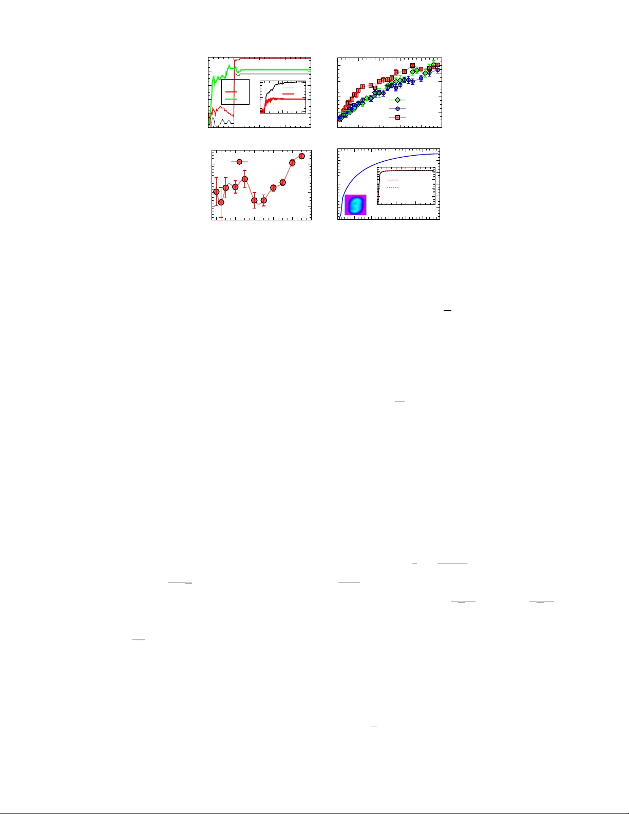
V ariational mean-field theory for training restricted Boltzmann mac hines with binary synapses Haiping Huang ∗ PMI L ab, Scho ol of Physics, Sun Y at-sen University, Guangzhou 510275, People’s R epublic of China (Dated: August 19, 2020) Unsup ervised learning requiring only ra w data is not only a fundamental function of the cerebral cortex, but also a foundation for a next generation of artificial neural net works. Ho wev er, a unified theoretical framew ork to treat sensory inputs, synapses and neural activity together is still lacking. The computational obstacle originates from the discrete nature of synapses, and complex interactions among these three essen tial elements of learning. Here, w e prop ose a v ariational mean-field theory in which the distribution of synaptic w eigh ts is considered. The unsup ervised learning can then be decomp osed in to tw o in tertwined steps: a maximization step is carried out as a gradien t ascen t of the lo wer-bound on the data log-likelihoo d, in which the synaptic w eight distribution is determined b y up dating v ariational parameters, and an exp ectation step is carried out as a message passing pro cedure on an equiv alen t or dual neural net work whose parameter is sp ecified b y the v ariational parameters of the weigh t distribution. Therefore, our framew ork provides insigh ts on how data (or sensory inputs), synapses and neural activities interact with each other to achiev e the goal of extracting statistical regularities in sensory inputs. This v ariational framew ork is verified in restricted Boltzmann mac hines with planted synaptic w eigh ts and handwritten-digits learning. Intr o duction. — Searching for hidden features in raw sensory inputs and thus a reasonable explanation of the inputs is a core function of natural intelligence [1, 2]. Sensory cortical circuits are able to extract useful information from noisy inputs because of unsup ervised synaptic plasticity shaping well-organized synaptic connections [3, 4]. F rom a neural netw ork p ersp ective, this kind of unsup ervised learning was mo deled by a simple tw o-la yer architecture, namely restricted Boltzmann mac hine (RBM) [5 – 7]. One lay er is used to receive the sensory inputs, thereb y b eing the visible lay er; while the other lay er serves as a hidden representation enco ding features in the inputs. No lateral connections exist within eac h lay er, whic h was designed to av oid costly sampling as in a fully-connected netw ork. Synaptic plasticity thus refers to the learning pro cess where the connection (weigh t) strengths b etw een these tw o la yers are adjusted to explain the sensory inputs. In the machine learning comm unity , this learning pro cess can be ac hieved b y the p opular truncated Gibbs sampling (also called contrast divergence algorithm [7]), which was particularly designed for con tinuous w eigh t v alues, and thus a gradien t ascen t of the data log-lik eliho o d is mathematically guaran teed [8]. Ho wev er, to model unsupervised learning with energy-efficient computation using low-precision synapses (weigh ts) [9, 10], the gradient-based metho d do es not apply due to the discreteness of synapses. An efficien t or v alid method of training RBM with lo w-precision w eigh ts w as th us thought to be out of reac h. Sev eral recent works studied computational principles of unsup ervised learning with lo w-precision synapses [11 – 19]. Due to the complexit y of analysis, these works fo cused on either of practical net work arc hitectures and the constraint of arbitrarily many data samples, thereb y failing to analyze the interaction among inputs, synaptic plasticity and neural activit y within a unified framework. Therefore, how this in teraction shap es the unsup ervised learning pro cess is still unkno wn, and moreov er, because a typical learning pro cedure in b oth biological neural netw orks and artificial ones must inv olve sensory inputs, synaptic plasticity and neural activity , understanding this in teraction b ecomes a k ey to unlo c k the blac k b ox of unsup ervised learning, which is not only a fundamental function of cerebral cortex [3, 4], but also a foundation for a next generation of artificial neural net w orks [2]. Here, we prop ose a v ariational principle that assumes a v ariational distribution of w eights. W e mo del the learning pro cess as a computation of the p osterior on the weigh t parameters given sensory inputs. The v ariational principle finds the b est approximation of the p osterior within a tractable parametric family . Remark ably , even though in the presence of b oth a generic RBM architecture and arbitrarily man y sensory data, the learning process improv es an appro ximate lo w er-b ound on the data log-lik eliho o d. Therefore, our v ariational principle ov ercomes the computational obstacle previously thought to b e c hallenging, op ening a new path tow ards understanding how sensory data, synapses and neurons interact with each other during unsup ervised learning. In particular, this principle can b e used to test h yp otheses or predictions drawn from theoretical studies of random models of unsupervised learning [11 – 19]. Mo del. — In this study , we use the RBM defined abov e with arbitrarily many hidden neurons (the left panel of Fig. 1) to learn hidden features in M input data samples, which are raw unlab eled data specified by { σ a } M a =1 . Each data sample is specified by an Ising-like spin configuration σ = { σ i = ± 1 } N i =1 where N is the size of an input sample ∗ Electronic address: huanghp7@gmail.sysu.edu.cn 2 i j k l { σ a } a = 1 M q λ i μ ( ξ i μ ) i j k l λ i μ / √ N Ξ μ z μ lea rni ng μ ν τ μ ν τ FIG. 1: (Color online) The schematic illustration of the v ariational mo del. N = 4 in this example (say , i, j, k and l ). The hidden la yer has P = 3 neurons. Note that ( N, P ) can be arbitr arily finite num b ers. (Left panel) The RBM arc hitecture receiv es data of M examples and encodes the hidden features of data in to synaptic connections (w eigh ts) in an unsupervised w a y . Here, w e tak e into account the weigh t uncertaint y captured by a v ariational distribution q λ iµ ( ξ µ i ) where ξ µ i refers to the connection b et ween sensory neuron i and hidden neuron µ , and λ iµ is the v ariational parameter. (Righ t panel) The equiv alen t RBM mo del where the connection b ecomes the v ariational parameter and the additional random field applied to a hidden neuron is determined b y the v ariance (Ξ 2 µ ) of the w eighted-sum input to that hidden neuron (see the main text). z µ is a standard normally distributed random v ariable. The equilibrium prop erties of the equiv alent RBM are used to adjust the v ariational parameter impro ving the low er-bound on the data log-lik eliho o d. (e.g., the n um b er of pixels in an image). The synaptic weigh ts are characterized by ξ , where each comp onent takes a binary v alue ( ± 1). The num b er of hidden neurons is defined b y P . The Boltzmann distribution of this RBM is given b y P ( σ ) = 1 Z ( ξ ) Q µ cosh( β X µ ) [20], where µ denotes the hidden neuron index, X µ ≡ 1 √ N ξ µ · σ , ξ µ is also called the receptiv e field of the µ -th hidden neuron, and Z ( ξ ) is the partition function dep ending on the joint set of all receptive fields ξ . Note that the hidden neurons’ activities ( ± 1) hav e b een marginalized out. The scaling factor 1 √ N ensures that the argumen t is of the order of unity . Supp osed that the data samples are generated from a RBM where the synaptic connections are randomly generated at first and then quenc hed. The inv erse-temp erature β th us tunes the noise level of generated data samples from the planted RBM. Then one standard test of any learning algorithm is to learn the planted synaptic connection matrix from the supplied data samples. T o further model the learning process , w e assume that the data samples are weakly-correlated [7, 12], e.g., sampled with a large in terv al. Therefore, we hav e the follo wing data probability: P ( { σ a } M a =1 | ξ ) = M Y a =1 1 Z ( ξ ) Y µ cosh( β X a µ ) , (1) where the sup erscript a in X a µ means that σ in X µ is replaced b y σ a . Finally , the learning process is mo deled by estimating the p osterior probability of the guessed synaptic w eights according to the Bay es’ rule [12, 18]: P ( ξ |{ σ a } M a =1 ) = Q a P ( σ a | ξ ) P ξ Q a P ( σ a | ξ ) = 1 Ω exp − M ln Z ( ξ ) + X a,µ ln cosh  β X a µ  ! , (2) where Ω is the partition function of the posterior, and a uniform prior for ξ is assumed, i.e., we hav e no prior kno wledge ab out the planted weigh ts. F or simplicity , w e use the same temp erature as that used to generate data. How ever, one obstacle to compute the p osterior probability is the nested partition function Z ( ξ ) ≡ P σ Q µ cosh( β X µ ) whic h in volv es an exponential computational complexit y . Except for a few sp ecial cases of one or t wo hidden neurons as studied in previous w orks [11 – 13, 15, 18, 19], the computation of the p osterior is impossible, let alone understanding the learning pro cess. This is the v ery motivation of this w ork that prop oses a new principled metho d to tackle this c hallenge for paving a wa y tow ards a scien tific understanding of a generic unsup ervised learning pro cess. A variational principle. — Rather than finding an approximate metho d to ev aluate the posterior, we use a v ariational distribution b elonging to the mean-field family [21 – 23], defined by q λ ( ξ ), and find the b est v ariational distribution to minimize the Kullback-Leibler (KL) divergence b etw een q λ ( ξ ) and P ( ξ |D ) where D denotes the data { σ a } , whic h is giv en b y KL( q λ ( ξ ) k P ( ξ |D )) = E ln q λ ( ξ ) − E ln P ( ξ |D ) = E ln q λ ( ξ ) − E ln P ( ξ , D ) + ln P ( D ) = − LB( q λ ) + ln P ( D ) , (3) 3 where KL( q k p ) ≡ D ln q p E q for tw o distributions— q and p , E denotes the exp ectation under the v ariational probability q λ where λ denotes the corresp onding v ariational parameter, and P ( ξ , D ) = P ( ξ |D ) P ( D ). Because of the non- negativit y of the KL div ergence, the low er-b ound on the data log-lik eliho o d is giv en b y LB( q λ ) ≡ E ln P ( ξ , D ) − E ln q λ ( ξ ) = E ln P ( D | ξ ) − KL( q λ ( ξ ) k P ( ξ )) , (4) where the argument of q λ is omitted when it is clear, and P ( ξ , D ) = P ( D | ξ ) P ( ξ ) where P ( ξ ) can b e treated as a prior probabilit y of weigh ts. The first term serv es as the exp ected log-likelihoo d of the data, while the second term is a regularization term. The first term encourages the v ariational distribution to explain the observ ed data (maximizing the exp ected log-likelihoo d of the data), while the second term encourages the approximate p osterior to match the prior. Therefore, the v ariational ob jectiv e in Eq. (4) tak es into account the balance b et ween likelihoo d and prior [23]. The learning pro cess is no w interpreted as finding the v ariational parameter λ that improv es the low er-b ound on the data log-lik eliho o d. The low er-b ound is tight once q λ matc hes P ( ξ |D ). T o proceed, we assume a factorized (across individual weigh ts) prior probabilit y parameterized by m ≡ { m iµ } : P ( ξ ) = Q i,µ h 1+ m iµ 2 δ ξ µ i , +1 + 1 − m iµ 2 δ ξ µ i , − 1 i where δ x,y denotes the Kronec ker delta function, and m iµ defines the mean of the synaptic strength from visible neuron i to hidden one µ (Fig. 1) [24, 25]. F or simplicity , w e also parameterize the v ariational distribution in the same form but with different means sp ecified by λ . The v ariational distribution is giv en by q λ ( ξ ) = Q i,µ h 1+ λ iµ 2 δ ξ µ i , +1 + 1 − λ iµ 2 δ ξ µ i , − 1 i . Hence the weigh t uncertain t y can be explicitly captured by the v ariational distribution, in contrast to the p oint-estimate in a usual contrast div ergence algorithm for contin uous w eights. This form w as also recently used in supervised learning of p erceptron mo dels [26, 27]. According to Eq. (1), w e can write ln P ( D | ξ ) explicitly and insert it into the low er-b ound, then w e get LB( q λ ) = − KL( q λ ( ξ ) k P ( ξ )) + E " X a,µ ln cosh( β X a µ ) − M ln Z ( ξ ) # . (5) The v ariational parameter λ is ac hieved by optimizing the low er-b ound through gradien t ascent, defined by ∆ λ = η ∇ λ LB( q λ ) where η is a learning rate. Before ev aluating the gradient, we need to calculate the regularization and log-lik eliho o d terms. Due to the factorization assumption, the regularization term can b e exactly computed as − KL( q λ ( ξ ) k P ( ξ )) = X x = ± 1 X i,µ [ S ( z , y ) − S ( z , z )] , (6) where z = 1+ λ iµ x 2 , y = 1+ m iµ x 2 , and S ( z , y ) ≡ z ln y . The exp ected log-lik eliho o d term is still difficult to estimate without any appro ximations. How ever, based on the fact that the v ariational distribution q λ is factorized, we assume that X a µ in volv es a sum of a large num b er of nearly indep enden t random v ariables and th us follo ws a Gaussian distribution N ( G a µ , Ξ 2 µ ), where the mean and v ariance can b e computed resp ectively by G a µ = 1 √ N P i ∈ ∂ µ λ iµ σ a i , and Ξ 2 µ = 1 N P i ∈ ∂ µ (1 − λ 2 iµ ), where i ∈ ∂ µ denotes all incoming neurons in to the µ -th hidden neuron. In this form, the uncertaint y of weigh ts on the pro vided data D has b een incorp orated in to this approximation given a large v alue of N . Giv en one sensory input, sa y σ a , the weigh ted-sum X a µ is conditionally indep endent [7]. It then follo ws that the exp ected log-lik eliho o d can b e approximated by a Mon te-Carlo estimation [28]: E " X a,µ ln cosh( β X a µ ) − M ln Z ( ξ ) # = 1 B 1 X a,µ,s ln cosh  β G a µ + β Ξ µ z s µ  − M B 2 X s ln X σ Y µ cosh  β G µ + β Ξ µ z s µ  , (7) where s denotes the index for a Monte-Carlo sample, z s µ is a standard normal random v ariable, B 1 and B 2 denote the n umber of Monte-Carlo samples, and G µ is defined by G a µ without the symbol a . In terestingly , the partition-function part of the exp ected log-lik eliho o d reduces to an equiv alen t RBM mo del (the right panel of Fig. 1) whose synaptic 4 KL 0 0.02 0.04 0.06 0.08 0.1 0.12 learning step 0 10 20 30 40 50 60 ( d ) ( d ) (d) (d) LB 0 1 2 3 4 0 20 40 60 test data training data 0 100 200 0 100 200 KL LB 0 0.2 0.4 0.6 0.8 1 0 50 100 150 200 Q 1 Q 2 Q 3 learning step overlap with ground truth (a) (a) overlap with ground truth 0.7 0.75 0.8 0.85 0.9 0.95 c 0 0.2 0.4 0.6 0.8 1 N=100, M=500 (c) (c) overlap with ground truth 0 0.2 0.4 0.6 0.8 data density α 0 1 2 3 4 5 c=0, P=2 c=0, P=3 c=0.3, P=2 (b) (b) FIG. 2: (Color online) Learning performance in planted RBM mo dels ( N = 100) and real datasets ( N = 784). The inv erse temp erature β = 1. Each learning step indicates all synapses are updated once. B 1 = B 2 = 1000. Here, the Kullback-Leibler div ergence refers to KL( q λ ( ξ ) k P ( ξ )), and the approximate low er-b ound of the data likelihoo d (Eqs. (5-7)) has been subtracted b y its starting v alue. (a) Learning tra jectories of RBM mo dels with P = 3 and orthogonal planted receptiv e field vectors of three hidden neurons ( M = 500). The inset shows evolution of the Kullback-Leibler divergence and appro ximate lo wer-bound. (b) Typical learning p erformance in planted RBM models as a function of data density α = M N . The learning p erformance is estimated at the 200-th step. Each mark er in the plot indicates the av erage ov er ten independent realizations of the mo del, with the error bar indicating the standard deviation. The theoretical threshold α thr = 1 for c = 0 [12, 13] and α thr = 0 . 596 for c = 0 . 3 [18]. (c) Learning p erformance versus correlation c with P = 2 and M = 500. The av erage is done o ver ten indep enden t realizations. (d) Learning tra jectories (KL and LB p er mo del-parameter) of RBM mo dels with P = 100 for structured (handwritten digits, th us N = 784) inputs of M = 1000 images (another 1000 images for test). B 1 = B 2 = 500. A lo calized v ariational parameter map (within the receptive field) is also shown. connections are no w replaced by the v ariational parameter λ scaled by √ N , and an additional quenched random field is introduced for each individual hidden neuron as Ξ µ z s µ due to the fluctuation of the weigh ted-sum input. This surprising transformation makes estimation of the original computational hard partition function in Eq. (5) tractable, as the cavit y metho d developed for a RBM [20] can be directly applied. In brief, a ca vit y probability or message P i → µ ( σ i ) without considering the µ -th hidden neuron can b e written into a closed-form iteration [29]. The fixed-p oint messages can b e used to estimate the partition function and other thermo dynamic quantities related to learning [29]. Another b enefit is that the resulting expression in Eq. (7) is amenable to the v ariational inference, i.e., gradient estimation. One can then deriv e the gradient ascent form ula to up date the v ariational parameter as λ t +1 iµ = λ t iµ + η ∆ iµ , where t denotes the learning step, and ∆ iµ is decomposed into three parts [29], given by ∆ iµ = ∆ Reg iµ + ∆ D iµ − ∆ Eq iµ , (8) where the first term stems from the regularization, namely ∆ Reg iµ ≡ P x = ± 1 x 2  ln 1+ xm iµ 1+ xλ iµ − 1  , the second data- dep enden t term ∆ D iµ ≡ β B 1 √ N P a,s σ a i tanh( β G a µ + β Ξ µ z s µ ) − β 2 λ iµ N B 1 P a,s  1 − tanh 2  β G a µ + β Ξ µ z s µ  , and the final mo del-dep endent term ∆ Eq iµ is estimated from the equiv alen t RBM mo del, giv en by M β √ N B 2 P s h C iµ − λ iµ z s µ √ N Ξ µ ˆ m µ i , where C iµ and ˆ m µ define the correlation b etw een visible and hidden neurons, and mean activities of hidden neurons, resp ectiv ely . These tw o thermo dynamic quantities are estimated under the Boltzmann measure of the equiv alent mo del P eq ( σ ) = 1 Z s eq Q µ cosh  β G µ + β Ξ µ z s µ  b y the message passing pro cedure. Note that | λ iµ | 6 1, and ξ µ i can b e deco ded as ξ µ i = sgn( λ iµ ), so-called maximizer of the p osterior marginals [30]. R esults. — W e first test our v ariational framework on plan ted RBM mo dels. More precisely , we first generate a RBM mo del whose synaptic weigh ts are randomly generated with a sp ecified correlation lev el c . The correlation-free case of c = 0 corresp onds to the orthogonal weigh t vectors of hidden neurons. Based on this RBM mo del with planted ground truth, a collection of data samples is prepared from Gibbs samplings of the mo del [7, 18]. These data samples are finally used as sensory inputs to our v ariational learning algorithm, with the goal of reconstructing the ground truth. The learning performance is measured by the ov erlap Q µ = 1 N P N i =1 ξ µ, prd i ξ µ, plt i , quan tifying the similarit y b et ween predicted and planted weigh ts. 5 T ypical b ehavior of the prop osed v ariational mean-field framework is shown in Fig. 2. The v ariational learning framew ork is able to recov er the ground truth, even in the case of three or more hidden neurons, which w as previously out of reac h, confirming that the v ariational mean-field theory is capable of capturing the complex interaction among sensory inputs, synaptic plasticity and neural activities. Most interestingly , there app ears a permutation-symmetry- brok en phenomenon in inferred synaptic weigh ts, whic h is shown by the observ ation that when we carry out a p erm utation op eration to receptiv e fields at an intermediate step (e.g., 50-th step), the o verlap with the ground truth can hav e a significant quan titative c hange (Fig. 2 (a)). The permutation-symmetry-brok en phase indeed exists as also theoretically prov ed in a t wo-hidden-neuron case [18]. The sim ulation results of our new v ariational framework add further evidences to this fundamental phenomenon, thereby making testing theoretical predictions of simple mo dels p ossible in more generic arc hitectures. Fig. 2 (a) shows that the KL divergence b etw een the v ariational p osterior and the prior gro ws with learning, demonstrating that our v ariational principle is able to search for a biased probabilit y of weigh ts. Note that in the algorithm w e do not assume an y prior knowledge ab out the w eight v ectors, or m iµ = 0 for all ( iµ ). How ever, the algorithm itself tak es the v ariability of the data samples into accoun t, driving the up date of the v ariational parameter to wards the ground truth, as indicated b y the saturation of the KL divergence. In addition, the appro ximate low er- b ound on the data log-lik eliho o d also gro ws with learning, suggesting that the v ariational mean-field framew ork indeed impro ves the appro ximate bound. It is clear that in the correlation-free case, the learning threshold do es not dep end on the n umber of hidden neurons ( P = 3 or P = 2), in accord with the recen t theoretical work [18] which explained that the underlying ph ysics is the partition function factorization. F urthermore, the correlation lev el decreases the threshold [18, 19], as also verified in curren t simulation results (Fig. 2 (b)). The threshold is rounded b y the finite size of the system. Below the threshold, a random-guess phase ( λ = 0) dominates the learning. Ab ov e the threshold, there app ears sp ontaneous symmetry breaking corresponding to concept-formation in unsup ervised learning [11, 12]. Although w e restrict the v ariational distribution to be in the mean-field family , the learning performance shows robustness to different planted correlation levels (Fig. 2(c)), consisten t with p opular c hoices of mean-field p osterior in deep learning [24 – 27, 31]. The v ariational principle searches for the b est approximate p osterior minimizing the KL div ergence in Eq. (3). It is thus reasonable that by adjusting the v ariational parameters, giv en enough data, the true w eights can be recov ered such that the probability distance is minimized. Finally , we apply the proposed framew ork to the MNIST dataset [32] (Fig. 2 (d)). W e clearly see that the original uniform prior is not preferred, th us the KL div ergence increases until a highly biased (non-uniform) probability of w eight configurations is reac hed. The learned highly-structured receptive fields can provide informative priors for fine-tuning deep neural netw orks [27, 33]. A detailed study is left for our future w orks. Meanwhile, the approximate lo wer-bound for b oth training and test (unseen) datasets increases un til saturation. Therefore, our framework is also promising in studying structured real dataset, esp ecially for extracting or verifying principles of unsup ervised learning [11 – 19]. Conclusion. — Although training and understanding of neural netw orks with low-precision weigh ts and activ ations b ecomes increasingly imp ortant [10, 26], a unified theoretical framework to treat sensory inputs, synapses and neural activit y together is still lac king, and thus the conceptual adv ance con tributed by our v ariational mean-field theory pro vides a route tow ards an in-depth understanding of unsup ervised learning in a principled probabilistic framework. In this framew ork, the synaptic w eight is no longer treated to be deterministic, but rather, it is sub ject to a v ariational distribution where the v ariational parameter, mean synaptic activit y level, is adjusted by an exp ectation-maximization- lik e mec hanism [34]. The gradien t ascen t of the appro ximate lo wer-bound behav es as an M-step at the synaptic activit y lev el, while the E-step at the neural activity level is carried out b y a fully-distributed message passing procedure on an e quiv alent neural net work whose netw ork parameters are determined in turn by the v ariational parameters. These t wo steps as a k ey to unsup ervised learning are unified into a single equation (Eq. (8)), providing insigh ts on how data (or sensory inputs), synapses and neurons shap e the unsupervised learning. In terestingly , this v ariational principle marrying gradien t ascent and message passing shares the similar spirit to the free-energy principle prop osed for explaining action, p erception and learning in the brain [35]. The prop osed v ariational mean-field theory for challenging discrete synapses in unsup ervised learning encourages dev eloping theory-grounded neuromorphic algorithms on neural net works with lo w-precision yet robust synapses and activ ations [9, 10]. Last but not the least, this framework op ens a new w ay to test the h yp othesis that unsupervised learning can be interpreted as breaking differen t t yp es of inheren t symmetry in a data-driv en sp ontaneous manner [18, 19], in a general setting, i.e., neural net work arc hitectures with arbitrarily many hidden neurons, and hidden la yers. 6 Ac knowledgmen ts This research was supp orted by the start-up budget 74130-18831109 of the 100-talent- program of Sun Y at-sen Univ ersity , and the NSFC (Grant No. 11805284). Supplemen tal Material App endix A: Mean-field estimation of the partition function of the equiv alent mo del for learning In this supplemen tal material, w e briefly summarize the mean-field estimation of the partition function of the equiv alent mo del as follo ws. T ec hnical details to derive these results based on the ca vity metho d hav e b een given in a series of works [12, 20]. This estimation provides a practical pro cedure called message passing w orking on single instances of the RBM, whic h is efficien t for a practical learning. W e first write the partition function for a Mon te-Carlo sample indexed by s as follo ws, Z s eq = X σ Y µ cosh  β G µ + β Ξ µ z s µ  , (S1) where G µ and Ξ µ are defined b y G µ = 1 √ N P i ∈ ∂ µ λ iµ σ i and Ξ 2 µ = 1 N P i ∈ ∂ µ (1 − λ 2 iµ ), resp ectively . Therefore, in the equiv alent RBM, λ iµ √ N acts as a contin uous w eight, and H µ ≡ Ξ µ z s µ acts a quenc hed random field applied to the µ -th hidden neuron in the equiv alen t RBM. First, the interaction b et ween visible and hidden neurons is of the order O ( 1 √ N ) and th us weak, then the cavit y appro ximation taking only correlations around a factor in the pro duct of Eq. (S1) leads to the following self-consisten t ca vity iteration: P i → ν ( σ i ) = 1 Z i → ν Y µ ∈ ∂ i \ ν ˆ P µ → i (S2a) ˆ P µ → i ( σ i ) = X { σ j | j ∈ ∂ µ \ i } cosh X j ∈ ∂ µ \ i β λ j µ σ j √ N + β λ iµ σ i √ N + β H µ ! Y j ∈ ∂ µ \ i P j → µ ( σ j ) , (S2b) where P i → ν ( σ i ) denotes the ca vity probability for σ i giv en that only the ν -th hidden neuron is remov ed (this is what the cavit y means), while ˆ P µ → i ( σ i ) summarizes all contributions around the factor µ when the v alue of σ i is given. Z i → ν is a normalization constan t for P i → ν ( σ i ). Note that the concept of cavit y is required for using the factorization of the join t probability of neural activities to write do wn the abov e closed-form iterativ e equation on the graphical mo del where the visible neuron acts as a v ariable no de, and the hidden neuron acts as a factor/function node in a factor-graph represen tation of the model [20, 36]. The resulting iterative equation is also named the b elief propagation in computer science communit y [37]. How ever, it is still not easy to ev aluate ˆ P µ → i ( σ i ) without further appro ximations, due to the intractable summation in Eq. (S2b). By noting that the term in Eq. (S2b)— P j ∈ ∂ µ \ i β λ j µ σ j √ N in volv es a sum of a large n umber of nearly-indep enden t random terms, one can apply the cen tral-limit-theorem as an appro ximation whose justification can b e made in practical learning exp erimen ts. Then the original intractable summation can b e replaced by an integral in volving Gaussian random v ariables. Therefore, the ca vity magnetization m i → ν = P σ i = ± 1 σ i P i → ν ( σ i ) under the measure of the cavit y probabilit y can b e readily obtained as m i → ν = tanh   X µ ∈ ∂ i \ ν u µ → i   , (S3a) u µ → i = tanh − 1  tanh( β χ µ → i + β H µ ) tanh( β λ iµ / √ N )  , (S3b) where µ ∈ ∂ i \ ν indicates all factors around the visible neuron i excluding the factor indexed by ν . m i → µ can b e in terpreted as the message passing from visible neuron to hidden neuron (Fig. 1), while u µ → i denotes the ca vity bias in terpreted as the message passing from hidden neuron to visible neuron. The mean of the Gaussian distribution appro ximation under the central-limit-theorem is given b y χ µ → i ≡ 1 √ N P j ∈ ∂ µ \ i λ j µ m j → µ collecting all messages 7 except those from i around the factor µ , weigh ted by their corresp onding v ariational parameters, and H µ denotes the quenc hed random field expressed as Ξ µ z s µ . Because of weak in teractions, this message passing equation is able to conv erge ev en in a few steps. Then the log-partition-function (so-called free energy) can b e readily constructed based on the visible neuron’s contribution F i and the factor’s contribution F µ , as ln Z = P i F i − ( N − 1) P µ F µ where the subtraction remov es the double counting of the contribution from the first term [38]. F i and F µ are giv en resp ectiv ely b y F i = ln X σ i Y µ ∈ ∂ i ˆ P µ → i ( σ i ) = X µ ∈ ∂ i h β 2 Λ 2 µ → i / 2 + ln cosh  β χ µ → i + β H µ + β λ iµ / √ N i + ln   1 + Y µ ∈ ∂ i e − 2 u µ → i   , (S4a) F µ = ln Z d% µ cosh ( β % µ + β H µ ) N ( % µ ; χ µ , Λ 2 µ ) = β 2 Λ 2 µ / 2 + ln cosh ( β χ µ + β H µ ) , (S4b) where Λ 2 µ → i ≡ 1 N P j ∈ ∂ µ \ i λ 2 j µ (1 − m 2 j → µ ), Λ 2 µ ≡ 1 N P j ∈ ∂ µ λ 2 j µ (1 − m 2 j → µ ), and χ µ ≡ 1 √ N P i ∈ ∂ µ λ iµ m i → µ . Note that χ µ and G µ are intrinsically different, b ecause the former describ es the equilibrium prop erties of the equiv alent RBM with fixed λ iµ (the right panel of Fig. 1 in the main text), while the latter captures the statistics under the v ariational distribution giv en the sensory input (the left panel of Fig. 1 in the main text). W e finally remark that the free energy is computed using the cavit y approximation, the lo w er-b ound of the data log-lik eliho o d is th us an approximate estimation of the original intractable lo wer-bound (Eq. (5) in the main text). App endix B: Deriv ations of gradients of the data log-likelihoo d low er-b ound Finally , let us ev aluate the gradien t of the low er-b ound. First, the gradien t of the regularization term with respect to the v ariational parameter is obtained as − ∂ ∂ λ iµ KL( q λ ( ξ ) k P ( ξ )) = X x = ± 1 x 2  ln 1 + xm iµ 1 + xλ iµ − 1  . (S1) It is clear that this term v anishes when the v ariational distribution is exactly matched to the prior. Second, the gradien t of the first term in the exp ected log-lik eliho o d (Eq. (7) in the main text) can be written as ∂ ∂ λ iµ E " X a,µ ln cosh( β X a µ ) # ' β B 1 √ N X a,s σ a i tanh( β G a µ + β Ξ µ z s µ ) − β 2 λ iµ N B 1 X a,s  1 − tanh 2  β G a µ + β Ξ µ z s µ  . (S2) Lastly , the gradien t of the second term in the exp ected log-lik eliho o d can b e derived as ∂ ∂ λ iµ E ln Z ( ξ ) ' β √ N B 2 X s  σ i tanh( β G µ + β Ξ µ z s µ )  − β λ iµ N B 2 X s  z s µ Ξ µ  tanh  β G µ + β Ξ µ z s µ   , = β √ N B 2 X s " C iµ − λ iµ z s µ √ N Ξ µ ˆ m µ # , (S3) where the expectation h·i means an a v erage under the Boltzmann measure of the equiv alent mo del P eq ( σ ) = 1 Z s eq Q µ cosh  β G µ + β Ξ µ z s µ  , C iµ and ˆ m µ th us define the correlation b etw een visible and hidden neurons, and mean activities of hidden neurons, resp ectiv ely . Interestingly , these tw o macroscopic thermo dynamic quantities can b e ev al- uated from the fixed p oint of the message passing equation (Eq. (S3)). In terested readers can find technical details 8 in our previous w ork [20]. Here we summarize the result as follows, m i = tanh   X µ ∈ ∂ i u µ → i   , (S4a) ˆ m µ = Z D z tanh( β ˜ χ µ + β H µ + β ˜ Λ µ z ) , (S4b) C iµ = ˆ m µ m i + β λ iµ √ N (1 − m 2 i ) A µ , (S4c) A µ = 1 − Z D z tanh 2 ( β ˜ χ µ + β H µ + β ˜ Λ µ z ) , (S4d) where D z ≡ e − z 2 / 2 / √ 2 π dz , ˜ χ µ ≡ 1 √ N P i ∈ ∂ µ λ iµ m i , and ˜ Λ 2 µ ≡ 1 N P i ∈ ∂ µ λ 2 iµ (1 − m 2 i ). m i is the magnetization (mean activity) of the visible neuron and can thus b e read off from the fixed p oint of the message passing equation. ˆ m µ ≡ * tanh P i ∈ ∂ µ β λ iµ σ i √ N + β H µ !+ whic h can b e easily estimated by using the central-limit theorem once again and then calculating a Gaussian integral. The computation of the correlation C iµ is a bit tricky . W e first define an auxiliary quantit y ˆ C iµ = C iµ − ˆ m µ m i , then compute the summation P i ∈ ∂ µ β λ iµ √ N ˆ C iµ as follo ws, X i ∈ ∂ µ β λ iµ √ N ˆ C iµ = h tanh( β % µ + β H µ ) β % µ i − ˆ m µ β ˜ χ µ , = Z d% µ N ( % µ ; ˜ χ µ , ˜ Λ 2 µ ) tanh( β % µ + β H µ )( β % µ ) − β ˆ m µ ˜ χ µ , = Z D z tanh( β ˜ χ µ + β H µ + β ˜ Λ µ z )( β ˜ χ µ + β ˜ Λ µ z ) − β ˆ m µ ˜ χ µ , = β 2 ˜ Λ 2 µ Z D z 1 − tanh 2  β ˜ χ µ + β H µ + β ˜ Λ µ z  ! , (S5) where we define % µ ≡ P i ∈ ∂ µ λ iµ √ N σ i , and C iµ ≡ h tanh( β % µ + β H µ ) σ i i by definition. F rom the last equality of Eq. (S5), w e can easily get ˆ C iµ = β λ iµ √ N (1 − m 2 i ) A µ , from which the correlation C iµ is obtained. Collecting all three parts of the gradient, we arrive at the gradient ascent form ula to update the v ariational parameter as λ t +1 iµ = λ t iµ + η ∆ iµ , where t denotes the learning step, and ∆ iµ is giv en by ∆ iµ = X x = ± 1 x 2  ln 1 + xm iµ 1 + xλ iµ − 1  + β B 1 √ N X a,s σ a i tanh( β G a µ + β Ξ µ z s µ ) − β 2 λ iµ N B 1 X a,s  1 − tanh 2  β G a µ + β Ξ µ z s µ  − M β √ N B 2 X s " C iµ − λ iµ z s µ √ N Ξ µ ˆ m µ # . (S6) Note that | λ iµ | 6 1, and ξ µ i can be deco ded as ξ µ i = sgn( λ iµ ). W e finally remark that although the message passing algorithm con verges fast to ev aluate the equilibrium properties of the dual RBM, there exist other methods, e.g., Gibbs sampling [7] or high-temperature expansion [39], for ac hieving the same goal. [1] D. Hassabis, D. Kumaran, C. Summerfield, and M. Botvinick, Neuron 95 , 245 (2017). [2] A. M. Zador, Nature Communications 10 , 3770 (2019). [3] D. Marr, Pro ceedings of the Roy al So ciety of London B: Biological Sciences 176 , 161 (1970). [4] H. Barlow, Neural Computation 1 , 295 (1989). [5] P . Smolensky (MIT Press, Cambridge, MA, USA, 1986), chap. Information Pro cessing in Dynamical Systems: F oundations of Harmon y Theory , pp. 194–281. 9 [6] Y. F reund and D. Haussler, T ech. Rep., Santa Cruz, CA, USA (1994). [7] G. Hinton, Neural Computation 14 , 1771 (2002). [8] Y. Bengio and O. Delalleau, Neural Comput. 21 , 1601 (2009). [9] S. K. Esser, R. Appuswam y , P . Merolla, J. V. Arthur, and D. S. Mo dha, in A dvanc es in Neur al Information Pr o c essing Systems 28 , edited by C. Cortes, N. D. La wrence, D. D. Lee, M. Sugiy ama, and R. Garnett (Curran Asso ciates, Inc., 2015), pp. 1117–1125. [10] I. Hubara, M. Courbariaux, D. Soudry , R. El-Y aniv, and Y. Bengio, J. Mach. Learn. Res. 18 , 6869 (2017). [11] H. Huang and T. T oy oizumi, Ph ys. Rev. E 94 , 062310 (2016). [12] H. Huang, Journal of Statistical Mechanics: Theory and Experiment 2017 , 053302 (2017). [13] A. Barra, G. Genov ese, P . Sollic h, and D. T an tari, Phys. Rev. E 96 , 042156 (2017). [14] J. T ubiana and R. Monasson, Phys. Rev. Lett. 118 , 138301 (2017). [15] H. Huang, Journal of Physics A: Mathematical and Theoretical 51 , 08L T01 (2018). [16] A. Barra, G. Genov ese, P . Sollic h, and D. T an tari, Phys. Rev. E 97 , 022310 (2018). [17] A. Decelle, S. Hwang, J. Rocchi, and D. T an tari, arXiv:1906.11988 (2019). [18] T. Hou, K. Y. M. W ong, and H. Huang, Journal of Physics A: Mathematical and Theoretical 52 , 414001 (2019). [19] T. Hou and H. Huang, arXiv:1911.02344 (2019). [20] H. Huang and T. T oy oizumi, Ph ys. Rev. E 91 , 050101 (2015). [21] L. K. Saul, T. Jaakkola, and M. I. Jordan, J. Artif. In t. Res. 4 , 61 (1996). [22] M. I. Jordan, Z. Ghahramani, T. S. Jaakkola, and L. K. Saul, Machine Learning 37 , 183 (1999). [23] D. M. Blei, A. Kucukelbir, and J. D. McAuliffe, Journal of the American Statistical Asso ciation 112 , 859 (2017). [24] C. Blundell, J. Cornebise, K. Kavuk cuoglu, and D. Wierstra, in Pr o c e e dings of the 32Nd International Confer enc e on International Conferenc e on Machine L e arning - V olume 37 (JMLR.org, 2015), ICML’15, pp. 1613–1622. [25] J. M. Hern´ andez-Lobato and R. P . Adams, in Pr o c e edings of the 32Nd International Confer enc e on International Conferenc e on Machine L e arning - V olume 37 (JMLR.org, 2015), ICML’15, pp. 1861–1869. [26] C. Baldassi, F. Gerace, H. J. Kapp en, C. Lucib ello, L. Saglietti, E. T artaglione, and R. Zecchina, Ph ys. Rev. Lett. 120 , 268103 (2018). [27] O. Shay er, D. Levi, and E. F eta ya, arXiv:1710.07739 (2017). [28] S. Mohamed, M. Rosca, M. Figurnov, and A. Mnih, arXiv:1906.10652 (2019). [29] See supplemen tal material at http://... for technical details of the mean-field estimation of the partition function of the equiv alent mo del and the deriv ations of gradients for learning. [30] H. Nishimori, Statistic al Physics of Spin Glasses and Information Pr o c essing: An Intr o duction (Oxford Universit y Press, Oxford, 2001). [31] S. F arquhar, L. Smith, and Y. Gal, arXiv:2002.03704 (2020). [32] Y. LeCun, The MNIST database of handwritten digits, retrieved from h ttp://yann.lecun.com/exdb/mnist. [33] G. Hinton, S. Osindero, and Y. T eh, Neural Computation 18 , 1527 (2006). [34] P . Mehta, M. Buko v, C.-H. W ang, A. G. Day , C. Richardson, C. K. Fisher, and D. J. Sch wab, Physics Reports 810 , 1 (2019). [35] K. F riston, Nature Reviews Neuroscience 11 , 127 (2010). [36] F. R. Kschisc hang, B. J. F rey , and H.-A. Lo eliger, IEEE T rans. Inf. Theory 47 , 498 (2001). [37] J. S. Y edidia, W. T. F reeman, and Y. W eiss, IEEE T rans Inf Theory 51 , 2282 (2005). [38] M. M´ ezard and G. Parisi, Eur. Phys. J. B 20 , 217 (2001). [39] E. W. T ramel, M. Gabri´ e, A. Mano el, F. Caltagirone, and F. Krzak ala, Phys. Rev. X 8 , 041006 (2018).