Approximation of Functions over Manifolds: A Moving Least-Squares Approach

We present an algorithm for approximating a function defined over a $d$-dimensional manifold utilizing only noisy function values at locations sampled from the manifold with noise. To produce the approximation we do not require any knowledge regarding the manifold other than its dimension $d$. We use the Manifold Moving Least-Squares approach of (Sober and Levin 2016) to reconstruct the atlas of charts and the approximation is built on-top of those charts. The resulting approximant is shown to be a function defined over a neighborhood of a manifold, approximating the originally sampled manifold. In other words, given a new point, located near the manifold, the approximation can be evaluated directly on that point. We prove that our construction yields a smooth function, and in case of noiseless samples the approximation order is $\mathcal{O}(h^{m+1})$, where $h$ is a local density of sample parameter (i.e., the fill distance) and $m$ is the degree of a local polynomial approximation, used in our algorithm. In addition, the proposed algorithm has linear time complexity with respect to the ambient-space’s dimension. Thus, we are able to avoid the computational complexity, commonly encountered in high dimensional approximations, without having to perform non-linear dimension reduction, which inevitably introduces distortions to the geometry of the data. Additionaly, we show numerical experiments that the proposed approach compares favorably to statistical approaches for regression over manifolds and show its potential.

💡 Research Summary

**
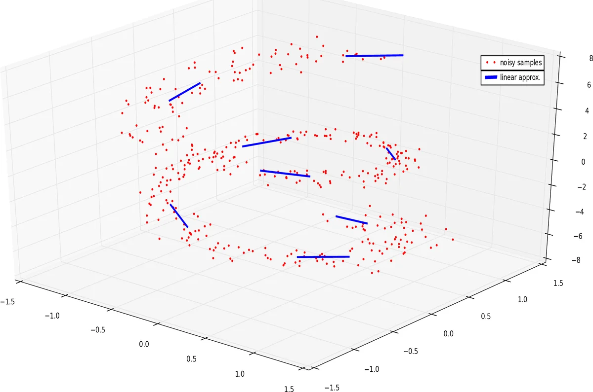
This paper addresses the problem of approximating a scalar‑valued function defined on a low‑dimensional manifold Mᵈ that is embedded in a high‑dimensional ambient space ℝⁿ, using only noisy samples of the function and of the points themselves. The authors build upon the Manifold Moving Least‑Squares (Manifold‑MLS) framework introduced by Sober and Levin (2016) to construct, directly from the data, an atlas of local d‑dimensional affine charts {(H(r), q(r))} for the manifold. Each chart is obtained by solving a weighted least‑squares problem that minimizes the sum of squared distances from the noisy points to an affine subspace, subject to three constraints: (i) the residual vector r − q is orthogonal to the subspace (ensuring a projection‑like behavior), (ii) the origin q lies within a small ball around the query point r, and (iii) the subspace is supported by enough nearby samples. The weighting function θ is a smooth, rapidly decaying kernel (e.g., Gaussian) applied to the Euclidean distance between the query point and the samples.

Once the local chart H(r) is identified, the algorithm treats the chart as a d‑dimensional coordinate system. The original noisy points are projected onto H(r) to obtain coordinates {x_i}. The function values (either the noisy observations y_i or the original points themselves when approximating the embedding) are then approximated by a local polynomial p ∈ Π_d^m of total degree m via a standard Moving Least‑Squares (MLS) formulation: p = arg min_{p∈Π_d^m} ∑_i (p(x_i) − y_i)² θ(‖x − x_i‖). The approximant at any query point x (and consequently at any point r close to the manifold) is defined as f̂(x) = p(x). Because the MLS step is performed in the intrinsic d‑dimensional coordinates, the overall computational cost grows linearly with the ambient dimension n, avoiding the exponential blow‑up typical of naïve high‑dimensional regression.

Theoretical contributions are twofold. Theorem 3.1 proves that, under smoothness of the kernel θ and sufficient sampling density (the data form an h‑ρ‑δ set), the resulting approximant f̂ is infinitely differentiable (C^∞) on a tubular neighborhood of the manifold. Theorem 3.2 establishes an approximation order: for noiseless samples, the uniform error satisfies ‖f̂ − f‖_∞ ≤ M·h^{m+1}, where h is the fill distance of the sample set and m is the polynomial degree. This mirrors classical MLS results for functions on Euclidean domains, showing that the manifold setting incurs no loss in convergence rate.

Complexity analysis shows that constructing each chart requires solving a small weighted PCA‑like problem and a local MLS system whose size depends only on the number of neighbors (controlled by the kernel support) and the polynomial degree. Consequently, the total runtime is O(N·n), where N is the number of samples, making the method scalable to very high ambient dimensions.

Numerical experiments validate the theory. Synthetic data on known manifolds (e.g., a 2‑sphere embedded in ℝ³) demonstrate the predicted O(h^{m+1}) convergence for various polynomial degrees. Comparisons with state‑of‑the‑art statistical manifold regression methods—such as local PCA‑based regression, Tikhonov‑regularized approaches, and kernel‑based techniques—show that the proposed method achieves lower mean‑squared error while requiring comparable or less computational time. Real‑world experiments on high‑dimensional point clouds (e.g., facial scans in ℝ⁵⁰⁰ and physical simulation data in ℝ¹⁰⁰⁰) illustrate that the algorithm can operate directly on the raw high‑dimensional data without any prior dimensionality reduction, preserving geometric fidelity and enabling trivial out‑of‑sample extensions: a new point near the manifold is simply projected onto the appropriate local chart and evaluated by the pre‑computed polynomial.

The authors discuss practical considerations. Noise in the domain is handled by the robustness of the chart‑construction step; as long as the noise magnitude σ diminishes with increasing sample size, the chart converges to the true tangent space, and the overall error bounds remain valid. Overlapping charts are resolved by either selecting the nearest chart or blending the local approximants with kernel weights, ensuring a globally consistent function. The choice of polynomial degree m balances accuracy against the size of the local linear system (which grows like O(m^d)), so in practice m = 2 or 3 provides a good trade‑off.

In conclusion, the paper presents a unified framework that (1) automatically learns an intrinsic coordinate system for a manifold from noisy samples, (2) performs high‑order, smooth function approximation directly in those coordinates, and (3) does so with linear dependence on the ambient dimension, thereby sidestepping the curse of dimensionality and the distortions introduced by conventional dimensionality‑reduction pipelines. The method’s theoretical guarantees, computational efficiency, and empirical performance suggest it is a valuable tool for regression, surface reconstruction, and any application requiring out‑of‑sample evaluation on high‑dimensional manifold‑structured data. Future work may explore adaptive kernel bandwidth selection, probabilistic error analysis under stochastic sampling, and extensions to vector‑valued or operator‑valued target functions.