Lyapunov Event-triggered Stabilization with a Known Convergence Rate

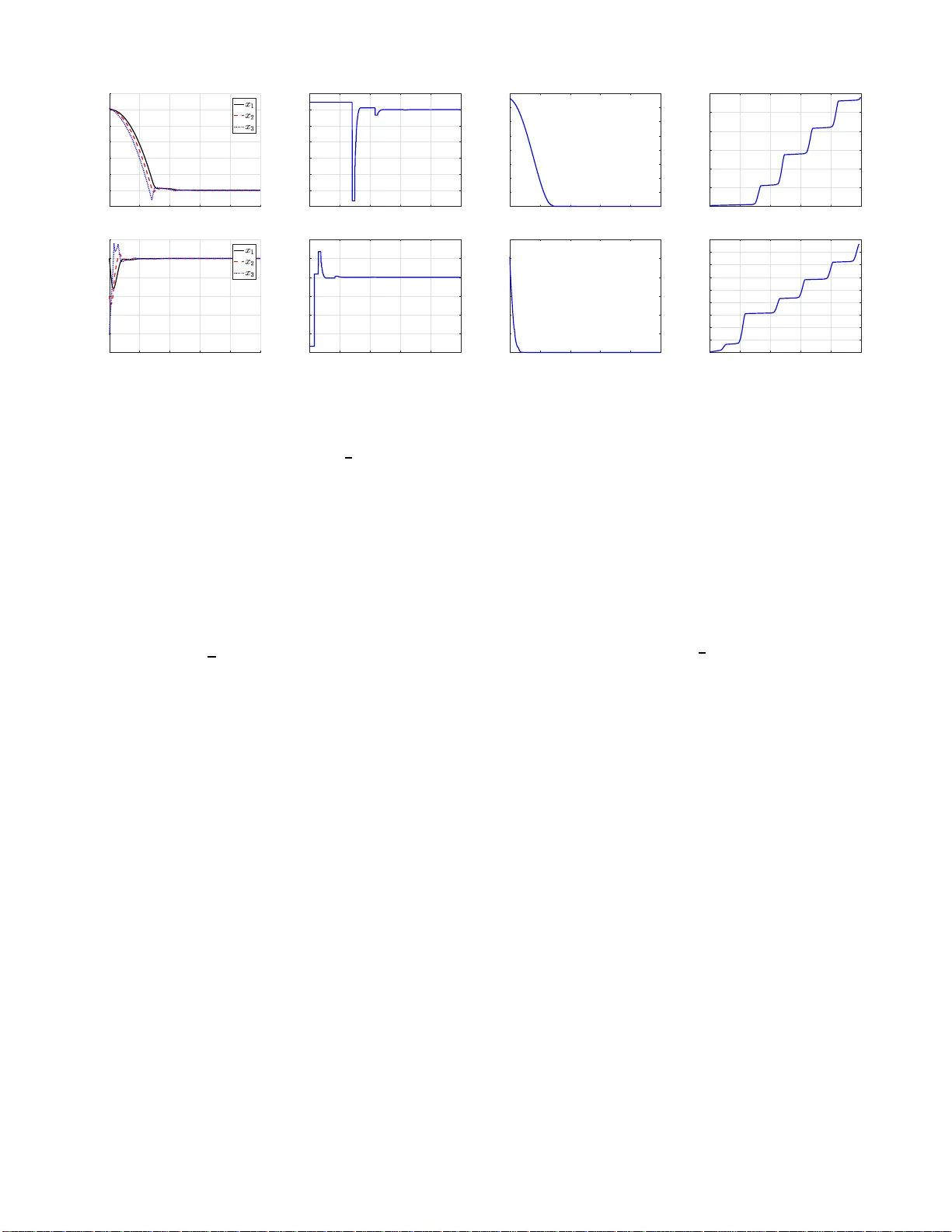
1 L yapunov Ev ent-triggere d Stabiliza tion with a Kno wn Con v er g ence Rate Anton V . Proskurnikov , Senior Member , IEEE a nd Manuel Mazo Jr ., Senior Membe r , IEEE Abstract —A constructive tool of nonlinear contro l systems de- sign, the method of Control L yapunov Functions (CLF) has f oun d numerous appl ications i n stab i lization problems for continuous- time, discrete-time and hybrid systems. In this paper , we address the fundamental question: given a CLF , corresponding to the continuous-time controller with some predeﬁned (e.g . exponential) con vergence rate, can t h e same conv ergence rate be provided by an ev ent-triggered controller? Under certain assumptions, we gi ve an afﬁrmative answer to this question and sh ow that the corresponding ev ent-based controllers pro vide positive dwell- times between the consecutive events. Furthermore, we prov e the existence of self- trigger ed and periodic ev ent-triggered con- trollers, providing stabilization with a known conv ergence rate. Key words — Control L yapunov Function, Event-triggered Control, Stabilization, Nonlin ear Systems I . I N T R O D U C T I O N The seminal idea to use th e seco nd L yapu nov method as a too l of control design [2] has naturally lead to the idea of control L yapunov Func tion (CLF). A CLF is a fu n ction that becomes a L yapun ov fun ction of the closed-loop system under an appr opriate ( usually , non- u nique) choice o f the co ntroller . The fu ndamen tal Artstein theor e m [3] states that the existence of a CLF is ne cessary an d sufﬁcient for stabilization of a general non lin ear sy stem by a “relaxed” controller, m apping the system’ s state in to a prob a bility measur e. For an afﬁne uncon stra in ed system, a usual static stabilizin g contr oller can always be found, as shown in the seminal work [4]. In g eneral, to ﬁnd a CLF for a giv en contr ol system is a non-tr ivial pr oblem since the set of CLFs may have a very sophisticated structur e , e.g. be d isconnected [5]. Howe ver , in some importan t situations a CLF can be explicitly found. Examples includ e some h omogen eous systems [6], feed back- linearizable, passive or feedb ack-passive systems [7], [8] an d cascaded sy stems [9], for which both CLFs and stabilizin g controller s can be delivered by the backstepping an d forwar d- ing pro cedures [ 10], [11]. The CLF method has recently been The authors are with Delft Center for Systems and Control, Delft Uni versi ty of T echnology , The Netherlands. E-mail: anton.p. 1982@ieee.org; m.mazo@tudelf t.nl The work is supported by NWO Domain TT W , Netherlands, under the project T TW#13712 “From Indivi dual Automated V ehicles to Cooperati ve Tra fﬁc Manage ment – predicting the beneﬁt s of automate d drivi ng through on-road human beha vior assessment and traf ﬁc ﬂow models” (IA V T RM). It is also partially funded by the project SENTIENT funded by the European Researc h Council (ERC) und er the EU’ s Horizon 2020 research and innov ation programme (ERC-StG 2017, #755953). A special ca se of Theore m 1 (dealin g with expone ntiall y stabilizing CLF) was pre sented [1] on the 21 st A CM Conference on Hybrid Syste ms Compu- tatio n and Cont rol (HSCC’2018), Porto, Portugal, April 11-13, 2018. empowered by the de velopment of algorith ms and software f or conv ex optimization [1 2], [1 3] an d gen e tic progr amming [14]. Now adays the meth od of CLF is r ecognized as a powerful tool in nonlinear control systems design [8], [10], [11]. A CLF giv es a solutio n to the Ham ilton-Jacobi- Bellman equatio n for an ap propr iate pe r forman c e index, giving a solu tion to the in verse optimality p roblem [15]. A n other num erical method to co m pute CLFs [16] emp loys the so-called Zu bov equation. The me thod of CLF h as been extended to uncertain [15], [1 7], discrete-time [18], time-d elay [1 9] an d hy brid systems [20], [21]. Combining CLFs an d Co n trol Barrier Function s (CBFs), correct-b y-design contr ollers for stabilization of constrained (“safety-critica l” ) systems h av e been pro posed [22]–[2 4 ]. For continuo us-time system s, CLF-based co ntrollers ar e also continuo us-time. Their implementa tio n o n digital platf orms requires to intro duce tim e samp ling. T he simplest appr oach is based o n emulation of the co ntinuou s-time fe edback by a discrete-time c o ntrol, sam p led at a hig h r a te. Rigor ous stability analysis of the resulting sampled -time systems is hig hly n on- trivial; we refer the r eader to [25] f o r a detailed sur vey o f the existing metho ds. A more gen eral framework to sample- time c o ntrol d esign, ba sed on a direct d iscretization of the nonlinear contr ol system and appr oximating it by a nonlin ear discrete-time inclusion, has been de veloped in [26]–[ 2 8]. T his method allows to d esign con trollers that cannot be directly redesigned from co ntinuous- tim e algorith m s, but th e relev a nt design procedu res and stability analy sis are sophisticated. The necessity to use comm unication, compu ta tio nal and power resources pa r simoniously has moti vated to study digital controller s tha t are based on event-trigger ed samp ling, wh ich has a number of adv antages over classical time- triggered control [29]–[33]. Event-trigg ered contro l stra tegies can be efﬁciently an a lyzed b y using the theories of hy brid sys- tems [33]–[35], switching systems [36], delayed systems [37], [38] and im pulsiv e systems [39]. It shou ld be noticed that the ev ent-trigge red samp ling is aperiodic and, unlike the cla ssical time-trigger ed designs, the inter-sampling inter val need not necessarily be sufﬁciently small: the contro l can be fro zen for a long time, provided that the b ehavior of the system is satisfactory an d req uires n o in tervention. On the other hand, with event-triggered samp lin g one has to p r ove th e existence of positive dwell time between consecutive ev ents: even thoug h mathematically any non -Zeno trajectory is admissible, in real- time control system s the samplin g rate is alw ays limited. A natural qu estion arises whether the existence of a CLF makes it possible to d esign an ev ent-trigge r ed contro ller . In a few situations, the answer is known to be afﬁrmativ e. T h e most studied is the case wher e the CLF ap pears to be a so called ISS Lyapunov function [30], [33] and allows to prove 2 the in put-to-state stab ility (ISS) o f the closed-loop sy stem with respect to measuremen t errors. A more rece nt result from [ 40] relaxes the ISS cond ition to a strong er version of usual asymptotic stability , howe ver the control algorithm from [40], in gener al, does n ot en sure the absence of Zeno solu tions. Another appro a c h, based o n So n tag’ s u niversal for mula [4] has been prop osed in [4 1], [4 2]. All of these results imp ose limitations, d iscussed in detail in Section II. In p articular, the estimation of the convergence rate fo r the meth ods pro posed in [40]–[42] is a non-trivial pro blem. In many situations a CLF can be designe d th at provid es some known conver gence rate (e.g. expon entially stabilizing CLFs [ 1], [21]) in co ntinuou s time. A natur al question arises wheth e r event-based controllers can p rovide the sam e (or an a r bitrarily close) con vergence rate. In this pap er , we give an afﬁrmative answer to this fundam ental que stion . Under natural a ssum ptions, we design an event-triggered con tr oller , pr oviding a k nown conver gence rate an d a positive dwell time b e twe en co nsecutive events. Furthermo re, w e design self-triggered an d period ic ev ent- triggered controllers th at simplify real-time task scheduling . The p aper is organ ized as follows. Section II giv es the deﬁnition of CLF and r e la te d concep ts and sets up the pro blem of event-trigger e d stab ilization with a predeﬁn e d con vergence rate. Th e solution to this problem , being the ma in result of the paper, is offered in Sectio n III, where ev ent-trigg ered, self- triggered and periodic ev ent-trigge red stabilizin g co ntrollers are designed. In Section IV, the main results are illustrated b y numerical examples. Section V conclu des the p aper . Appendix contains some techn ical pro ofs and discussion on the key assumption in th e main result. I I . P R E L I M I NA R I E S A N D P RO B L E M S E T U P Hencefor th R m × n stands for the set of m × n real matr ices, R n = R n × 1 . Given a fun ction G : R n → R m that m aps x ∈ R n into G ( x ) = ( G 1 ( x ) , . . . , G m ( x )) ⊤ ∈ R m , we use G ′ ( x ) =  ∂ G i ( x ) ∂ x j  ∈ R m × n to denote its Jaco b ian matrix. A. Contr ol Lyapunov functions in stab ilizatio n pr oblems T o simplify matters, henceforth we de al with the p r oblem of global asymp totic stabilization. Consider the following con trol system ˙ x ( t ) = F ( x ( t ) , u ( t )) , t ≥ 0 , (1) where x ( t ) ∈ R d stands f or the state vector and u ( t ) ∈ U ⊆ R m is the con trol input (the case U = R m correspo n ds to the absence o f input con straints). Our g oal is to ﬁnd a controller u ( · ) = U ( x ( · )) , where U : x ( · ) 7→ u ( · ) is some cau sal (non - anticipating) o perator, such that for any x (0) ∈ R d the so lu tion to the clo sed -loop system is for ward comp lete (exists up to t = + ∞ ) an d co n verges to the uniq u e equilibriu m x = 0 x ( t ) − − − → t →∞ 0 ∀ x (0) ∈ R d , F (0 , U (0)) = 0 . (2) W e now give the deﬁnition of CLF . Following [4], we hencefo rth assume CLFs to be smooth, radially unbo unded (or pr oper ) and p ositiv e deﬁnite. Deﬁnition 1 : [4] A C 1 -smooth function V : R d → R is called a contr ol Lyapunov function (CLF) V (0) = 0 , V ( x ) > 0 ∀ x 6 = 0 , lim | x |→∞ V ( x ) = ∞ ; (3) inf u ∈ U V ′ ( x ) F ( x, u ) < 0 ∀ x 6 = 0 . (4) The condition (4 ), o bviously , can be r eformulate d a s follows ∀ x 6 = 0 ∃ u ( x ) ∈ U such that V ′ ( x ) F ( x, u ( x )) < 0 . (5) If F ( x, u ) is Le besgue m easurable (e.g., contin uous), then the set { x 6 = 0 , u ∈ U : V ′ ( x ) F ( x, u ) < 0 } is also measurable and the Auman n me a surable selector theor em [43, The o rem 5.2] implies that the fun ction u ( x ) can be cho sen measur able; howe ver, it can be discon tinuous an d inf e asible (the closed- loop system has no solutio n for some initial condition ). Some systems (1) with co ntinuou s r ight-hand sides cann ot be stabi- lized by usual controller s in spite of the existence of a CLF , howe ver, they can b e stabilized by a “r e la xed” con trol [3] x 7→ v ( x ) , where v ( x ) is a pr obability distribution o n U . The situa tio n become s m uch simpler in the case o f afﬁne system (1) with F ( x, u ) = f ( x ) + g ( x ) u . Assuming that f : R d → R d and g : R d → R d × m are con tinuous an d U is conve x , the existence o f a CLF e n sures the p ossibility to design a co ntroller u = u ( x ) , where u : R d → U is continuo us ev erywhere except fo r, possibly , x = 0 [3]. While the orig inal proof f rom [3] was not fully constru cti ve, Sontag [4] has propo sed an explicit universal fo rmula, giving a br oad class of stabilizing controllers. Assuming that U = R m , let a ( x ) ∆ = V ′ ( x ) f ( x ) , b ( x ) ∆ = V ′ ( x ) g ( x ) . Then (4) mean s that a ( x ) < 0 whe nev er b ( x ) = 0 and x 6 = 0 . In the scalar ca se ( m = 1 ), Sontag’ s controller is u ( x ) = ( − a ( x )+ √ a ( x ) 2 + q ( b ( x ) ) b ( x ) b ( x ) , b ( x ) > 0 0 , otherwise. (6) Here q ( b ) is a continu ous fun c tio n, q (0) = 0 . It is shown [4 ] that th e control (6) is continu ous at any x 6 = 0 , m o reover , if a ( · ) , b ( · ) and q ( · ) ar e C k -smooth (respe c ti vely , re al analytic), the sam e holds fo r u ( · ) in the doma in R d \ { 0 } . Th e glo b al continuity requ ires an addition “small con trol” p roperty [4]. Similar c o ntrollers h av e be e n foun d for a more gener al case, where m > 1 and U is a closed ball in R m [44]. B. CLF and event-trigger ed contr ol Dealing with continu o us-time systems (1), the CLF-b ased controller u = U ( x ) is also continuous-time, an d its im plemen- tation o n digital platform s requ ires time-sampling . Formally , the contro l c ommand is com puted and sent to the plant at tim e instants t 0 = 0 < t 1 < . . . < t n < . . . a n d remain constant u ( t ) ≡ u n for t ∈ [ t n , t n +1 ) . The app roach broadly used in engin eering is to em u late the con tinuous-tim e feedback b y sufﬁciently fast perio dic o r aperiod ic sampling ( th e inter vals t n +1 − t n are small). W e refer the reader to [25] for the survey of existing results on stability under samp led-time con trol. 3 As an alternative to periodic sampling, meth ods of n on- unifor m event-b a sed samp ling hav e bee n prop o sed [29], [30]. W ith these methods, th e next sampling instant instan t t n +1 is triggered by some event, depend ing on the pr evious instant t n and the system’ s trajectory for t > t n . Special cases are self-trigger ed co ntrollers [45], [46], where t n +1 is determined by t n and x ( t n ) , and there is n o need to check tr ig gering condition s, and periodic even-triggered contro l [4 7], which requires to check the trig gering condition o nly period ica lly at times nτ . The advantages o f ev ent-trigge red c ontrol over traditional periodic contro l, in particular the economy o f com - munication an d e nergy resources, have been d iscussed in the recent papers [29]–[ 32]. Event-trigg ered con tr ol alg orithms are widespread in b iology , e.g. oscillator networks [48]. A natur al q uestion arises wh ether a co ntinuou s-tim e CLF can be employed to de sig n an event-trigger e d stabilizing controller . Up to no w , only a fe w results of th is type ha ve been reported in the literature. In [30], an event-triggere d contro ller requires the existence of a so-called I SS Lyapunov function V ( x ) and a contro ller u = k ( x ) , satisfy ing the cond itions α 1 ( | x | ) ≤ V ( x ) ≤ α 2 ( | x | ) ∀ x ∈ R d (7) V ′ ( x ) F ( x, k ( x + e )) ≤ − α 3 ( | x | ) + γ ( | e | ) ∀ x, e ∈ R d . ( 8) Here α i ( · ) ( i = 1 , 2 , 3 ) are K ∞ -functio n s 1 and the map pings k ( · ) : R d → R m , F ( · , · ) : R d × R m → R d , α − 1 3 ( · ) and γ ( · ) : R + → R + are assumed to be locally Lipschitz. Subsituting e = 0 into (8), one easily sh ows that the I SS L yapun ov f unction satisﬁes (4), b eing thus a spec ia l case of CLF; the cor respondin g f e e dback U ( x ) ∆ = k ( x ) no t o nly stabilizes the system, but in fact also provides its inp ut to state stability (I SS) with respe ct to the measurem ent er ror e . Th e ev ent-trigge red controller, offered in [3 0], is as fo llows u ( t ) = k ( x ( t n )) if t ∈ [ t n , t n +1 ) t 0 = 0 , t n +1 = inf { t > t n : γ ( | e ( t ) | ) = σα 3 ( | x ( t ) | ) } , e ( t ) = x ( t n ) − x ( t ) , σ = const ∈ (0 , 1) . (9) The co ntroller (9) guaran tees a positive dwell time between consecutive events τ = inf n ≥ 0 ( t n +1 − t n ) > 0 , wh ich is uniformly po siti ve fo r the solutions, starting in a compact set. Whereas the cond ition (8) holds for linear systems [30] and some polyn o mial systems [45], in genera l it is restrictive and not easy to verify . Another appr oach to CLF-based design of ev ent-trigge red co ntrollers h a s b een propo sed in [41], [ 42]. Discarding the I SS co n dition (8), this app roach is based on Sontag’ s theory [4] and inhe r its its basic assumptions: ﬁrst, th e system has to be afﬁne F ( x, u ) = f ( x ) + g ( x ) u , wh e re f , g ∈ C 1 , secon d, Sontag ’ s con troller is admissible ( u ( x ) ∈ U for any x ). The controllers from [41], [42] also provide p ositi vity of th e dwell time (“min imal inter-sampling interval”). An alternative event-trigger e d con tr ol algorith m, substan- tially relaxing the ISS con dition (8) an d app licable to non- afﬁne systems, h a s b een propo sed in [40] and requ ir es the existence of a CLF , satisfying ( 7) an d (8) with e = 0 V ′ ( x ) F ( x, k ( x )) ≤ − α 3 ( | x | ) . (10) 1 A funct ion α ( · ) belong s to the cl ass K ∞ if it is continu ous and strictl y increa sing wit h α (0) = 0 and li m s →∞ α ( s ) = ∞ . The events are tr ig gered in a way p roviding that V strictly decreases a lo ng any non - equilibriu m trajectory t n +1 = inf { t ≥ t n : V ′ ( x ( t )) F ( x ( t ) , u n ) = − µ ( | x ( t ) | ) } . (11) Here 0 < µ ( r ) < α 3 ( r ) for any r > 0 an d µ is K ∞ -functio n . As noticed in [40], this algo rithm in gener al does not p rovide dwell time positivity , an d may even lead to Zeno solution s. As will be discu ssed below , th e con ditions (7) and (10) entail an estimate fo r the CLF’ s conver gence rate . In this paper, we assume that the CLF satisﬁes a mo re general convergence rate con dition, and design an ev ent-trigg ered c ontroller that preserves the conv ergence rate and p rovides positive dwell time between consecu ti ve switchings. Also, we show th at f or each bound ed region o f th e state space, self-trigg ered and period ic ev ent-trigge red contro ller s exist th a t provide stability fo r any initial co n dition f rom this region. Our app roach substantially differs fr om th e previous works [30], [40]–[42], [45]. Un- like [30], [45], we do no t assume th at CLF satisﬁes the I SS condition (8). Un like [ 41], [42], the af ﬁn ity o f th e system is not needed, and the solu tion’ s c o n vergence rate can be explicitly estimated. Unlike [40], the dwell time positivity is e stab lished. C. CLF with kno wn conver gence rate Whereas the existence o f CLF typically allows to ﬁnd a stabilizing controller, it can p otentially b e un satisfactory du e to very slow convergence. Thro ughou t th e pap er , we assume that a CLF gives a controller with k n own conver gence rate. Deﬁnition 2 : Consider a continuo us f unction γ : [0; ∞ ) → [0; ∞ ) , suc h that γ ( v ) > 0 ∀ v > 0 (and he n ce γ (0) ≥ 0 ) . A function V ( x ) , satisfying (3), is said to b e a γ -stabilizin g CLF , if there exists a map U : R d → U , satisfying the conditio ns V ′ ( x ) F ( x, U ( x )) ≤ − γ ( V ( x )) ∀ x, F (0 , U (0)) = 0 . (12 ) Remark 1 : The condition (10), as well as the stro nger ISS condition (8), imply th at V is γ -stabilizing CLF with γ ( v ) = α 3 ◦ α − 1 2 ( v ) ( γ is co ntinuou s since α i are K ∞ -functio n s). In general, neither γ -CLF V ( x ) is a m onoton e fun ction of th e norm | x | , nor γ is mono tone. Hen ce (12) is mor e general than ( 1 0). No te that U ( · ) may be d iscontinuou s an d “infea sible” (the c lo sed-loop system m ay h ave no solutions). T o examine the b ehavior of solutions o f the closed-loop system, we introduce the fo llowing fu nction Γ : (0 , ∞ ) → R Γ( s ) ∆ = Z s 1 dv γ ( v ) , s > 0 . (13) The deﬁn itio n ( 13) imp lies that Γ( s ) is positive when s > 1 and negative fo r s < 1 . Since, Γ ′ ( s ) = 1 /γ ( s ) > 0 , Γ is increasing and hence the limits (possibly , inﬁnite) exist Γ ∆ = lim s → 0 Γ( s ) < 0 , Γ ∆ = lim s →∞ Γ( s ) > 0 . The inverse Γ − 1 : (Γ , Γ ) → (0 , ∞ ) is in creasing and C 1 - smooth. If Γ > −∞ , w e d e ﬁne Γ − 1 ( r ) ∆ = 0 f o r r ≤ Γ . T o und erstand the meaning of the fu nction Γ( s ) , consider now a special situation, where the equality in (1 2) is achieved V ′ ( x ) F ( x, U ( x )) = − γ ( V ( x )) ∀ x ∈ R d . (14) 4 The CLF V ( x ( t )) can b e treated as some “energy”, stored in the system at time t , whereas γ ( V ( x ( t ))) = − ˙ V ( x ( t )) ca n be treated as the energy dissipation rate or “power” con su med by th e clo sed-loop system (“ work” done by th e sy stem p er unit of time) with feedb ack u = U ( x ) . By noticing that d dt Γ( V ( x ( t )) = ˙ V ( x ( t )) /γ ( V ( x ( t )) = − 1 , th e functio n Γ may be con sidered as the “energy-time characteristics” of the system: it takes the system time t 1 = Γ( V 0 ) − Γ( V 1 ) to move from th e en ergy le vel V 0 = V ( x (0)) to the energy level V 1 . In g eneral, (1 2) im p lies an upp er boun d for a solu tio n. Proposition 1: Let the system (1) have a γ -stabilizing CLF V , correspon ding to the controller U . Let x ( t ) be a so lution to ˙ x ( t ) = F ( x ( t ) , u ( t )) , u ( t ) ∆ = U ( x ( t )) . (15) Then on the interval of the solu tion’ s existence the fun ction V ( t ) = V ( x ( t )) satisﬁes the fo llowing inequality 0 ≤ V ( t ) ≤ Γ − 1 (Γ( V (0)) − t ) . (16) Pr oof: If V ( t ) > 0 at any time when the solution exists, then ˙ V ( t ) = V ′ ( x ( t )) F ( x ( t ) , u ( t )) (12) ≤ − γ ( V ( t )) < 0 and d dt Γ( V ( t )) ≤ − 1 = ⇒ Γ( V ( t )) ≤ Γ( V (0)) − t, (17) which implies (16) since Γ − 1 is increasing. Suppose now that V ( t ) vanishes at some t ∈ [0 , δ ) , and let t 0 ≥ 0 be the ﬁrst such instant. By deﬁnition, fo r t ∈ [0 , t 0 ) one h as V ( t ) > 0 , which entails (17) an d (16). Since V is non -increasing , V ( t ) ≡ 0 for t ≥ t 0 , and th us (16) holds also for t ≥ t 0 . Corollary 1: If Γ > −∞ , then the solution of (15) co n- verges to 0 in ﬁnite time δ ∗ = Γ ( V ( x (0))) − Γ (provided th at it exists on [0 , δ ∗ ) . If Γ = −∞ and x ( t ) is a f orward complete solution to (1 5), then x ( t ) − − − → t →∞ 0 . Dependin g o n the ﬁnitene ss of Γ , Proposition (1) explicitly estimates e ither time or rate o f the CLF’ s conver gence to 0 . Example 1. Let γ ( v ) = κ v , wh ere κ > 0 is a con stant. In this case Γ( s ) = κ − 1 ln s , Γ = −∞ , Γ = ∞ , Γ − 1 ( r ) = e κ r . The γ -stabilizing CLF p rovides exponential stabilization (being a n E S-CLF [21]). The inequality (16) reduces to 0 ≤ V ( t ) ≤ exp  κ ( κ − 1 ln V (0) − t )  = V (0) e − κ t . (18) Example 2. Let γ ( v ) = κ v a with κ > 0 , a > 1 . W e have Γ( s ) = [ κ ( a − 1)] − 1 (1 − s 1 − a ) , Γ = −∞ , Γ = [ κ ( a − 1)] − 1 , Γ − 1 ( r ) = (1 − κ ( a − 1) r ) 1 / (1 − a ) , and (16) boils down to V ( t ) ≤  V (0) 1 − a + t κ ( a − 1)  1 1 − a . (19) Example 3. Let γ ( v ) = κ v a with κ > 0 , a < 1 . Similar to the case a > 1 , o ne h as Γ( s ) = [ κ ( a − 1)] − 1 (1 − s 1 − a ) and Γ − 1 ( r ) = (1 − κ ( a − 1 ) r ) 1 / (1 − a ) , h owe ver, Γ = [ κ ( a − 1)] − 1 > −∞ . The condition (16) again lead s to ( 19), howe ver, the righ t-hand side vanishes for t ≥ t 0 ∆ = κ (1 − a ) − 1 V (0) 1 − a , e.g. the solutio n converges in ﬁnite time t 0 . Example 3 shows that a CLF can g i ve a co ntroller, solving the pro b lem of ﬁnite-time stabilization. An event-triggered counterp art of such a co ntroller can be d esigned, using th e proced u re discussed in the n ext sectio n. Howe ver, the pro p erty of lo cal po siti vity of d well time does not hold for such a controller (see Rem ark 5), and thus the absen ce of Zen o trajectories does not follow fro m our main results. Fin ite-time ev ent-trigge red stabilization is thus beyond the sco pe of this paper, being a subject of ongoin g re sear ch. D. Pr oblem setup In this paper, we a ddress the following fun damental ques- tion: d o es the existence of a co ntinuou s-time γ -stabilizing CLF allo w to design an event-trigger e d m echanism, providing the same con vergence rate as the continuou s-time control u = U ( x ) ? Relax ing the latter req uirement, we seek for e vent- triggered controller s whose conver gence rates a re arbitrarily close to th e co nvergence rate of the continu ous-time contr oller . Problem. Assume that V is a γ -stabilizing CLF , wh ere γ ( v ) is a known fun ction, and σ ∈ (0 , 1) is a ﬁxed constant. Design an event-triggered contro ller , p roviding the follo wing co ndition ˙ V ( x ( t )) ≤ − σ γ ( V ( x ( t ))) ∀ t ≥ 0 . (20) Applying Propo sition 1 to ˜ γ ( s ) = σγ ( s ) (which co rrespond s to ˜ Γ( s ) = σ − 1 Γ( s ) ), it is shown that (20) entails that 0 ≤ V ( x ( t )) ≤ Γ − 1 (Γ( V ( x (0))) − σ t ) . (21) For instance, in the Ex ample 1 co nsidered above ( 21) imp lies exponential conver gence with expon e nt σ κ (that is, V ( t ) ≤ V (0) e − σ κ t ) (versus the rate κ in continu ous time). Remark 2 : In some situation s, the CLF serves not only as a L y apunov function , but also as a b a rrier certiﬁcate [22], ensuring that th e trajecto ries do not cross so m e “un safe” set D . For in stance, suppo se that fo r any poin t of th e bound ary ξ ∈ ∂ D one has V ( ξ ) ≥ v ∗ > 0 . Then for any initial condition beyond th e unsafe set’ s closure x (0) 6∈ D such that V ( x (0)) < v ∗ , th e solution of the co ntinuou s-time system (1 5) starting at x (0) can n ot cross the bo undary ∂ D and thu s cann ot enter the unsafe set. The event-triggered algorithm p roviding (20) preserves the latter property of the CLF and p r ovides thus safety for the afo remention ed class of initial conditio ns. I I I . E V E N T - T R I G G E R E D , S E L F - T R I G G E R E D A N D P E R I O D I C E V E N T - T R I G G E R E D C O N T RO L L E R D E S I G N S Hencefor th we supp ose that a con tin uous strictly positiv e function γ ( · ) , a γ -stabilizing CLF V ( x ) and the correspon d ing feedback map U : R d → U are ﬁxed. All algorith ms consider ed in this paper provide that u ( t ) ∈ U ( R d ) ; without lo ss of generality , we assume that U = U ( R d ) . W e are going to design an event-triggered algorithm that ensures (20). Th e input u ( t ) switches at sampling instants t 0 , t 1 , . . . , where t 0 = 0 and the next instants t n depend s o n th e solutio n , re m aining constan t u ( t ) ≡ u n = u ( t n ) on each samp ling in terval [ t n , t n +1 ) . A. The event-trigger ed con tr ol a lgorithm d esign The con dition (2 0) can be rewritten as W ( x ( t ) , u ( t )) ≤ − σ γ ( V ( x ( t )) , where the function W is deﬁn ed b y W ( x, u ) ∆ = V ′ ( x ) F ( x, u ) ∈ R , x ∈ R d , u ∈ U, (22) 5 At the initial instant t 0 = 0 , calculate the control inp ut u 0 ∆ = U ( x ( t 0 )) . If V ( x ( t 0 )) = 0 , then the system starts at the equ ilibrium point and stays there under the control input u ( t ) ≡ u 0 ∀ t ≥ t 0 . Otherwise, W ( x ( t 0 ) , u ( t 0 )) ≤ − γ ( V ( x ( t 0 ))) < − σ γ ( V ( x ( t 0 ))) due to (12), and hence for t sufﬁciently clo se to t 0 one has W ( x ( t ) , u 0 ) < − σ γ ( V ( x ( t ))) . The n ext sampling instant t 1 is the ﬁ rst time w h en W ( x ( t ) , u 0 ) = − σ γ ( V ( x ( t ))) , we fo rmally deﬁne t 1 = ∞ if such an in stant does n ot exist. If t 1 < ∞ , we r epeat th e procedu re, calculatin g the new control in p ut u 1 = U ( x ( t 1 )) . If V ( x ( t 1 )) = 0 , then the system has arrived at th e equilib rium, an d stays there un d er the contro l inp u t u ( t ) ≡ u 1 . Otherwise, W ( x ( t 1 ) , u ( t 1 )) (12) ≤ − γ ( V ( x ( t 1 ))) < − σ γ ( V ( x ( t 1 ))) . Hence for t close to t 1 one has W ( x ( t ) , u 1 ) < − σ γ ( V ( x ( t ))) . T h e next sampling instant t 2 is the ﬁrst time t > t 1 when W ( x ( t ) , u 1 ) = − σγ ( V ( x ( t ))) , we d eﬁne t 2 = ∞ if such an instant does not exist. Iterating this proced u re, the sequen ce of instants sampling t 0 < t 1 < . . . < t n < t n +1 < . . . is constru c ted in a way th at the contro l u ( t ) = u n ∆ = U ( x ( t n )) for t ∈ [ t n , t n +1 ) satisﬁes (12). If V ( x ( t n )) > 0 , t n +1 is th e ﬁrst time t > t n when W ( x ( t ) , u n ) = − σ γ ( V ( x ( t ))) . (23) The sequ ence of sampling instants termin ates if V ( x ( t n )) = 0 or (23) does not ho ld at any t > t n , in this case we formally deﬁne t n +1 = ∞ a n d the control is fro zen u ( t ) ≡ u n ∀ t > t n . The p rocedu r e just descr ib ed can be written as follows u ( t ) = U ( x ( t n )) ∀ t ∈ [ t n , t n +1 ) , t 0 = 0 , t n +1 =  inf { t > t n : (23) holds } , V ( x ( t n )) > 0 , ∞ , V ( x ( t n )) = 0 . (24) (where inf ∅ = + ∞ ), or in the following “pseu d ocode form ”. Algorithm (24) in the pseud ocode for m n ← 0 ; t n ← 0 ; u n ← U ( x (0)) ; while V ( x ( t n )) > 0 do repeat u ( t ) = u n ; ⊲ t is the curren t time until W ( x ( t ) , u n ) = − σ γ ( V ( x ( t ))) ; n ← n + 1 ; t n ← t ; u n ← U ( x ( t n ))) ; end while ; freeze u ( t ) ≡ U (0) ; ⊲ stay in the equilibriu m Remark 3 : I mplementatio n of Algorithm ( 2 4) d oes not r e - quire any closed-fo rm analytic e xpression for U ( x ) ; if suf ﬁces to h av e some numerical algorithm f or com p utation of the value u n = U ( x ( t n )) at a spe c iﬁc poin t x ( t n ) . Remark 4 : Triggering co ndition (23) is similar to the con - dition (11), em ployed by th e algor ithm fr om [4 0], howe ver, as explained in Remark 1, in gener a l the co nditions adop ted in [40] d o not hold. Further m ore, unlike [40], we giv e con di- tions fo r the positi v ity of dwell time (to be deﬁned below) and explicitly estimate the conv ergence r ate o f the algorith m. T o assure the practical applicability of the alg orithm (24), one has to p rove th at the solution of the closed-loop sys- tem is fo rward comp lete, addr essing th us two pr o blems. Th e ﬁrst prob lem, addressed in Su b section II I-B, is the solu tion existence betwee n two sampling instants: to sh ow that the ev ent (23) is detected earlier than th e solution to the following equation “explodes” (escapes from any compac t) ˙ x ( t ) = F ( x ( t ) , u n ) , u n = U ( x ( t n )) , t ≥ t n . (25) The second problem , addressed in Subsection III-C, is to sho w the impossibility of Ze n o solution s. Deﬁnition 3 : A solution to the clo sed-loop system (1),(2 4) is said to be Zeno , or exhibit Zeno b ehavior if the sequ ence of sampling in stants is inﬁnite and h as a limit t ∞ = lim n →∞ t n = sup n ≥ 0 t n < ∞ ; otherwise, the trajecto ry is said to b e non-Zeno . Although mathem a tically it can be p ossible to pr olong the solution beyond the time t ∞ [49], the practical implementation of algorithm (24) with Ze n o trajecto ries is problematic. Mo re- over , any real- tim e implemen tation of the algorith m im p oses an implicit restriction on the minimal time between two consecutive events, referred to as the solution’ s dwell-time . Since the contro l comm ands can not be com puted arbitrarily fast, in practice th e so lu tions with zero d well-time ar e also undesirab le, ev en if they ar e for ward complete. Deﬁnition 4 : The value T ( x 0 ) = inf n ≥ 0 ( t n +1 ( x 0 ) − t n ( x 0 )) is called the dwell-time or the minimal inter -sampling interval (MSI) [ 41] o f the solutio n. Algo rithm (24) provides locally uniformly po siti ve dwell-time if T is un iformly positive over all so lutions, star ting in a com pact set K : inf x 0 ∈K T ( x 0 ) > 0 . The p roof of locally u niform dwell-time p ositi vity a llows to design self-triggered and pe r iodic e vent- triggered mod iﬁca- tions of ( 24) that are discussed in Su bsections I II-D,E. Remark 5 : By deﬁnition of the dwell-time, t 1 − t 0 = t 1 ≥ T ( x (0)) . In particular, if U ( x (0)) 6 = U (0) , then x ( t ) 6 = 0 f or t ∈ [0 , T ( x (0)) (wh en x = 0 , the con trol h as to be switched to U (0) ). For instance, in the situation from Ex ample 3 from previous section , the solu tion ( if it exists) conv erges to 0 in time, p ropor tio nal to V ( x (0)) d ue to (2 1). Such a contro ller can pr ovid e the dwell-tim e positivity , but not lo cally unifor m positivity since T ( x 0 ) ≤ σ − 1 V ( x 0 ) → 0 as | x 0 | → 0 . Remark 5 may be illustrated by the simp le example of the system ˙ x = u an d a r e la y con trol U ( x ) = sgn x . Choosing V ( x ) = x 2 and γ ( v ) = 2 √ v , the event-triggere d algorithm (24) in fact coincid es with the co ntinuou s time control: the ﬁr st event is ﬁred at time t 0 and u 0 = sg n x 0 ; if x 0 6 = 0 , th e secon d event occurs a t t 1 = | x 0 | a nd u 1 = 0 . B. The inter-sampling beha v ior of solutions T o examine the solution s’ beh avior between two sampling instants, we introduce the aux iliary Cauchy problem ˙ ξ ( t ) = F ( ξ ( t ) , u ∗ ) , ξ (0 ) = ξ 0 , t ≥ 0 , (26) where u ∗ ∈ U . T o provide th e uniqu e solvability of (26), hencefo rth the following non- restrictiv e assumptio n is adopted . 6 Assumption 1 : For u ∗ ∈ U , the map F ( · , u ∗ ) is lo cally Lipschitz; in p articular, W ( · , u ∗ ) : R d → R is c o ntinuou s 2 . Proposition 2: Unde r Assumptio n 1, the Cauchy prob- lem (26) has the unique solution ξ ( t ) = ξ ( t | ξ 0 , u ∗ ) , which satisﬁes at least one of the following two cond itions holds 1) W ( ξ ( t ) , u ∗ ) > − σ γ ( V ( ξ ( t ))) for some t ≥ 0 ; 2) the solution is b ounded and for ward complete. Pr oof: The ﬁrst statement follows fr om the Picard- Lindel ¨ o f existence theo rem [8]. Assume tha t on the interval of th e solution ’ s existence we have ˙ V ( ξ ( t )) = W ( ξ ( t ) , u ∗ ) ≤ − σ γ ( V ( ξ ( t ))) (the ﬁrst cond ition d oes no t hold ). T hen V ( ξ ( t )) ≤ V ( ξ 0 ) , a nd hence ξ ( t ) also rem ains bou nded o n its interval of existence, and hence is fo rward complete. Corollary 2: Under Assumption 1, x ( t ) = ξ ( t − t + | x + , u ∗ ) is th e o n ly solu tion to the following Cauchy problem ˙ x ( t ) = F ( x ( t ) , u ∗ ) , x ( t + ) = x + , t ≥ t + , (27) where u ∗ ∈ U . If x + = 0 an d u ∗ = U (0) , then ξ ( t ) ≡ 0 . Corollary 2 allows to show th at the solution to th e closed- loop system (1),(24) exists and unique for any initial co n dition. One can show via indu ction o n n that the sequen ce { t n } is uniquely deﬁned by x (0) by noticing th at t 0 = 0 is u n iquely deﬁned an d if t n < ∞ , then the n ext in stant t n +1 ≤ ∞ depend s on ly on t n , x n , u n . If x n = 0 , then algorithm s stop s and t n +1 = ∞ . In view of Proposition 2, either ev ent (23) occurs a t some time t > t n (the ﬁrst suc h in stant is t n +1 < ∞ ), or the solution is well deﬁned on [ t n , ∞ ) and satisﬁes (20) (in which case t n +1 = ∞ ). In bo th situation s, the solution is well deﬁned o n th e n th samplin g interval [ t n , t n +1 ) . Corollary 3: Let Assump tion 1 h old. Then the sequ ence of samp ling instan ts { t n } in the algo rithm (24) is u niquely deﬁned by the in itial condition x (0) , and the solution between them is uniquely de ﬁn ed b y the formu la x ( t ) = ξ ( t − t n | x n , u n ) ∀ t ∈ [ t n , t n +1 ) . (28) where ξ ( t | ξ 0 , u ∗ ) stan d s for the solution to ( 26). Notice that th e solutio n is automatically fo rward c o mplete in the case where the sequence t n terminates (for some n , we have t n +1 = ∞ ). This however is not guaran teed for the case where inﬁnitely many e ven ts occur . T o exclude the possibility of Z eno b ehavior , add itional assumption s are required . C. Dwell time po sitivity In this subsection, we formu la te our ﬁrst main re su lt, namely , the criter io n of dwe ll time po sitivity in Algor ithm (2 4). This criterion re lies on several additional assum p tions. For any x ∗ ∈ R d and K ⊂ R d , denote B ( x ∗ ) ∆ = { x : V ( x ) ≤ V ( x ∗ ) } , B ( K ) ∆ = [ x ∗ ∈K B ( x ∗ ) . ( 29) Algorithm (24) implies that V ( x ( t )) is non-inc reasing due to (12), and h ence x ( t ) ∈ B ( x ( s )) for t ≥ s ≥ 0 . In 2 Recal l tha t V ∈ C 1 by deﬁnitio n of th e CLF particular, sets B ( x ∗ ) are forwar d in variant along the solutions of (1),(24). For any bou nded set K , B ( K ) is a lso boun ded since B ( K ) ⊆ { x : V ( x ) ≤ sup x ∗ ∈K V ( x ∗ ) } . According ly to Assumptio n 1, the following su premum is ﬁn ite κ ( x ∗ ) ∆ = sup x 1 ,x 2 ∈ B ( x ∗ ) x 1 6 = x 2 | F ( x 1 , U ( x ∗ )) − F ( x 2 , U ( x ∗ )) | | x 2 − x 1 | < ∞ (30) for any x ∗ (in the case where x ∗ = 0 and B ( x ∗ ) = { 0 } , let κ ( x ∗ ) ∆ = 0 ). W e adopt a stron ger version o f Assum ption 1. Assumption 2 : The L ip schitz constant κ ( x ∗ ) in (30) is a locally bounde d f unction of x ∗ . Assumption 2 holds, for instance, if the mapping U is locally bound ed and F ′ x ( x, u ) exists and is continuou s in x and u . Assumption 3 : The gradien t V ′ ( x ) is locally L ip schitz. Assumption 3 is a stronge r version of CLF’ s smoothness and ho ld s e.g. when V ∈ C 2 . Similar to (30), we intro duce the Lipschitz constant o f V ′ on th e compact set B ( x ∗ ) : ν ( x ∗ ) ∆ = sup x 1 ,x 2 ∈ B ( x ∗ ) x 1 6 = x 2 | V ′ ( x 1 ) − V ′ ( x 2 ) | | x 2 − x 1 | , ν (0) ∆ = 0 . (31) Assumption 3 im plies that ν is loca lly bou nded since f o r any com pact K th e set B ( K ) is b ounde d an d sup x ∗ ∈K ν ( x ∗ ) ≤ sup x 1 ,x 2 ∈ B ( K ) x 1 6 = x 2 | V ′ ( x 1 ) − V ′ ( x 2 ) | | x 2 − x 1 | < ∞ . Finally , we ad opt an assumption that allo ws to establish the relation betwe en the c on vergence rates of th e γ -CLF V ( x ( t )) under the co n tinuous-tim e control U = U ( x ) and the solution x ( t ) . Notice that (12) gives n o in formation about th e speed o f the solution’ s co n vergence since ˙ V ( x ) = V ′ ( x ) ˙ x ( t ) depend s only on the velocity’ s ˙ x ( t ) p rojection o n the gr adient vector V ′ ( x ) , whereas its transversal com ponent can be arbitrary . These transversal dyn amics can p otentially lead to very slow and “non- smooth” convergence, in the sense that | ˙ x ( t ) | ≫ | ˙ V ( x ( t )) | . As discussed in Ap pendix B, in such a situation the dwell-time positivity cannot b e proved. Denoting ¯ F ( x ) ∆ = F ( x, U ( x )) , and introducing the angle θ ( x ) between ¯ F ( x ) and V ′ ( x ) (Fig. 1), the de ﬁn ition of γ -CLF (1 2) imp lies that V ′ ( x ) = 0 = ⇒ x = 0 = ⇒ ¯ F ( x ) = 0 cos θ ( x ) < 0 ∀ x 6 = 0 . Our ﬁnal assumption req uires these con ditions to hold un i- formly in th e vicinity of x = 0 in the fo llowing sense. Assumption 4 : The γ -CLF V ( x ) and the corresp o nding controller U ( x ) satisfy th e following pr operties: | ¯ F ( x ) | ≤ M 1 ( x ) | V ′ ( x ) | ∀ x ∈ R d , cos θ ( x ) ≤ − M 2 ( x ) ∀ x ∈ R d \ { 0 } , (32) 7 Fig. 1: Illustration to Assump tion 4: the angle θ ( x ∗ ) where the f unctions M 1 , M 2 are, respectively , unifo r mly bound ed and u niformly strictly po siti ve o n any compact set. The inequ a lities (32) imply that the solution does no t oscillate n ear the equ ilibrium since | ¯ F ( x ) | → 0 as | x | → 0 , a n d the ang le b e twe en the vector s 3 ˙ x = ¯ F ( x ) and V ′ ( x ) re m ains strictly ob tuse as x → 0 , i.e. the ﬂow is not transversal to the CLF’ s gr a dient. Assumption 4 can be reformu lated as follows. Lemma 1: For a γ - CLF V , Assumption 4 holds if and only if a lo cally b o unded fun ction M ( x ) > 0 exists such that | V ′ ( x ) | | ¯ F ( x ) | + | ¯ F ( x ) | 2 ≤ M ( x ) | V ′ ( x ) ¯ F ( x ) | ∀ x ∈ R d . (33 ) Pr oof: For M ( x ) ∆ = (1 + M 1 ( x )) / M 2 ( x ) , (3 2) im p lies M ( x ) | V ′ ( x ) ¯ F ( x ) | = M ( x ) | co s θ ( x ) || V ′ ( x ) | | ¯ F ( x ) | (32) ≥ M ( x ) M 2 ( x ) | V ′ ( x ) | | ¯ F ( x ) | M M 2 =1+ M 1 ≥ ≥ | V ′ ( x ) | | ¯ F ( x ) | + M 1 ( x ) | V ′ ( x ) | | ¯ F ( x ) | (32) ≥ | V ′ ( x ) | | ¯ F ( x ) | + | ¯ F ( x ) | 2 , proving th us the “only if ” part. T o prove the “if ” par t, note that (33) an d (1 2) imply the inequa lities M ( x ) cos θ ( x ) = M ( x ) V ′ ( x ) ¯ F ( x ) | V ′ ( x ) | | ¯ F ( x ) | ≤ − 1 | ¯ F ( x ) | 2 ≤ M ( x ) | V ′ ( x ) ¯ F ( x ) | ≤ M ( x ) | V ′ ( x ) | | ¯ F ( x ) | , and hence ( 32) ho lds with M 1 = M and M 2 = 1 / M . W e n o t turn to the ke y problem of dwell time estimatio n for Algorithm (2 4). In v iew of ( 28), to estimate of th e time elapsed between con secutiv e e vents t n +1 − t n , it sufﬁces to stud y the behavior of the solutio n ξ ( t ) = ξ ( t | x ∗ , U ( x ∗ )) to the Cauchy problem ( 2 6) with ξ 0 = x ∗ 6 = 0 and u ∗ = U ( x ∗ ) , namely , to ﬁnd the ﬁrst in stant ¯ t suc h that W ( ξ ( ¯ t ) , u ∗ ) = − σ γ ( V ( ξ ( ¯ t ))) . The f ollowing lemma im plies that ¯ t ≥ τ ( x ∗ ) , wher e τ ( · ) is some fun c tion, uniformly strictly positive on any comp a ct set. Lemma 2: Let Assumptions 1-4 hold and γ ( · ) be either non-d ecreasing or C 1 . T hen a fun ction τ : R d → (0 , ∞ ) e xists, depend ing on σ, γ , κ , ν , M , that satisﬁes two con ditions: 1) τ ( · ) is u niformly strictly po siti ve o n any compact set; 2) for any x ∗ 6 = 0 , th e so lu tion ξ ( t ) = ξ ( t | x ∗ , U ( x ∗ )) is well-deﬁned o n the clo sed interval [0 , τ ( x ∗ )] an d W ( ξ ( t ) , U ( x ∗ )) < − σ γ ( V ( ξ ( t ))) ∀ t ∈ [0 , τ ( x ∗ )) . (34 ) 3 The inequali ty (12) implie s that both vectors are non-zero unless x 6 = 0 . Moreover , if the functions κ , ν , M are globally bo unded , γ ∈ C 1 and inf v ≥ 0 γ ′ ( v ) > −∞ , then inf x ∗ ∈ R d τ ( x ∗ ) > 0 . The p roof of Lemma 2 will be given in Append ix A; in this proo f th e exact expression f or τ ( · ) will be fo u nd, which in volves th e func tions γ , κ , ν, M . Note that Algorithm ( 2 4) does not employ τ ( · ) , wh ich is n eeded to estimate the d well time. Notice that for a ﬁxed x ∗ ∈ R d , th e value τ ( x ∗ ) = τ σ ( x ∗ ) m ay be considered as a fun ction of th e para m eter σ from (20). It can be shown that τ σ ( x ∗ ) → 0 as σ → 1 . In other word s, if the event-triggered alg orithm provide s the same conv ergence ra te as the co n tinuous-tim e c o ntrol, the d well time between con secu ti ve events vanishes. Le m ma 2 implies ou r main r esult. Theorem 1: Let the assumptio ns of Lemma 2 hold. Th en the following estimate fo r the dwe ll- time in (24) holds T ( x 0 ) ≥ τ min ( x 0 ) ∆ = inf x ∈ B ( x 0 ) τ ( x ) > 0 , (35) where τ ( x ) stan ds for the fun ction from Lemma 2. Th e dwell- time T is uniformly po sitive on any comp act. More over, if the functions κ , ν , M are glo bally bo unded , γ ∈ C 1 and inf v ≥ 0 γ ′ ( v ) > −∞ , then T is unifor mly strictly positiv e on R d . Pr oof: Notice ﬁrst that the f unction τ min from (35) is locally uniformly po siti ve on any com pact set K ⊆ R d since inf x 0 ∈K τ min ( x 0 ) = inf x ∈ B ( K ) τ ( x ) > 0 due to the bou ndedn ess o f the set B ( K ) an d local unifo rm positivity o f τ . Applying Lemma 2 to x ∗ = x n and using (28), one shows that if the n th ev ent is raised at the instant t n < ∞ , the next e vent cannot be ﬁred earlier than at time t n + τ ( x n ) . Since x n ∈ B ( x 0 ) , o ne has t n +1 ≥ t n + τ min ( x 0 ) , wh ich implies (35) b y deﬁn ition o f the dwell time T ( x 0 ) . D. Self-trigger ed a nd time- trigger ed stab ilizing con tr ol As has be e n already men tioned, Algo r ithm (24) requ ires neither fu ll knowledge of th e fun c tions κ , ν, M , nor even upper e stima te s fo r them . If such estimates are k nown, τ ( · ) from Lemma 2 can b e f o und explicitly (see Appen dix A), and algorithm (24) can be replaced by the self-trigger ed con troller: u ( t ) = U ( x ( t n )) , t ∈ [ t n , t n +1 ) , t 0 = 0 , t n +1 =  t n + τ ( x ( t n )) , V ( x ( t n )) > 0 ∞ , V ( x ( t n )) = 0 . (36) The a lg orithm (36) req uires to com p ute the value of τ ( x n ) at each step. Alterna ti vely , if a lower bound τ ∗ for th e value of τ min ( x 0 ) from (35) is known τ min ( x 0 ) ≥ τ ∗ > 0 , one may consider period ic or ap e r iodic time-trigger ed sampling u ( t ) = U ( x ( t n )) , t ∈ [ t n , t n +1 ) , t 0 = 0 , 0 < t n +1 − t n ≤ τ ∗ , lim n →∞ t n = ∞ . (37) Here the seq uence { t n } is in depend e nt of the trajecto r y; often t n = nτ 0 with some p eriod τ 0 ≤ τ ∗ . Remark 6 : Notice that to ﬁnd a lower estimate f or τ min ( x 0 ) , there is no n eed to k now the initial cond itio n x 0 8 (which can b e u ncertain); it sufﬁces to k now an up per bo und for the value of V ( x 0 ) , which d etermines th e set B ( x 0 ) . Lemma 2 and (28) yield in the following result. Theorem 2: Under the assump tions of Lemma 2, any solu- tion to the closed-loo p sy stem ( 1), (36) is forward complete and satisﬁes (20). T h e same ho lds f o r solutions to (1), (37), whose initial conditions satisfy the inequ a lity τ min ( x (0)) ≥ τ ∗ . Pr oof: Theorem 2 is proved very similar to Theorem 1, with th e on ly technical difference that (20) is not a u tomatically guaran tee d along the trajectories, and thus forward in variance of th e set B ( x 0 ) still h as to be proved. Using induc tio n on n = 0 , 1 . . . , we a re going to prove th at x ( t n ) ∈ B ( x (0)) for each n . The indu ction base n = 0 is obviou s. Assuming that x ( t n ) ∈ B ( x (0)) , we kn ow that t n +1 − t n ≤ τ ( x ( t n )) (in th e ca se o f (37) th is holds since τ min ( x 0 ) ≤ τ ( x ( t n )) ). Substituting x ∗ = x n to (34) an d using (28), one shows that (2 0) holds on each sampling interval [ t n , t n +1 ] , and thus x ( t n +1 ) ∈ B ( x ( t n )) . This proves the indu c tio n step, entailing also th a t b oth algorithms ensure (20). The solution thus re mains bo unded and is forward com plete ( t n → ∞ ). Remark 7 : As follows fro m Lemma 2, if the fu nctions κ , ν , M ar e globally bou nded, γ ∈ C 1 and inf v ≥ 0 γ ′ ( v ) > −∞ , then for 0 < τ ∗ < inf x 0 ∈ R d τ min ( x 0 ) the pe r iodic control (37) provides (2 0) for a ny initial co ndition. In other words, the sampled-time emulation of the co ntinuous feed back at a suf- ﬁciently high sampling rate ensures global stability of the closed-loo p system with a known convergence rate. Remark 8 : T he existing results on stability of non lin ear systems with sampled-tim e contro l (37) typically ad opt some continuity a ssum ptions o n the continuou s-time controller . One of the stand ard assump tions [5 0], [5 1] is the Lipschitz con tinu- ity of U ( · ) and uniform bounded ness of F ′ u ( x, u ) . Th e weakest assumption o f this type [ 5 2] req u ires 4 the m ap ( x, x ∗ ) 7→ F ( x, U ( x ∗ )) to be con tinuous (usu a lly , U h as to be continu ous). Theorem 2 does not rely on any of these condition s, howe ver , | F ( x, U ( x ) | = O ( | x | ) as | x | → 0 du e to Assum p tions 3 and 4. The latter co n dition fails to h old when the con tinuous-time control u = U ( x ) p rovides ﬁn ite- time stabilization [53], [ 5 4]. This agrees with Remark 5, explaining th at o ur procedu re of ev ent-trigg ered controller design canno t g uarantee loc a l unifor m dwell-time po siti v ity in the latter case. The strong advantage of the self-trigger ed and the period ic sampling algorith ms is th e possibility to schedule commun i- cation an d control tasks. Such algo r ithms are more convenient for real-tim e em bedded systems engin eering tha n the event- triggered contro ller (2 4), which req uires constan t mon itoring of the solu tio n x ( t ) an d p otentially can use the communic a tio n channel at any time. The d ownside of this is the necessity to estimate the in te r-sampling time τ ( · ) . The con servatism of such estimate s lead s to m ore data tran sm issions and contro l switchings th an the event-triggered contro ller (24) needs. 4 Notice that in [52], the continuous-t ime s ystem is exponent ially stable with quadrat ic L yapuno v function V ( x ) , whereas the sampled-ti me system is only asymptotic ally stable (without an y explic it estimate for the con verge nce rate). E. P erio d ic event-trigger ed stabilization A combination of the event-triggered and pe r iodic samplin g, inheriting th e advantages of both app roaches, is referr e d to as p eriodic event-triggered co n trol [47], [55]. Unlike usual ev ent-trigge red contr ol, the tr iggering condition is checked periodically with some ﬁxed pe r iod h > 0 , i.e. the co ntrol input can b e r ecalculated o nly at time k h , where k = 0 , 1 , . . . . This automatica lly exclud es the p ossibility o f Zen o behavior (obviously , t n +1 − t n ≥ h > 0 ) and simpliﬁes scheduling of the computa tio nal and co mmunicatio n task s. The main d ifﬁculty in design ing the period ic event-triggered controller is to ﬁnd such a triggerin g condition that its v alidity at time k h auto matically implies the desired contro l goal (20) on the interval [ kh, ( k + 1 ) h ] , even if the con tr ol inpu t at time t = k h remain s unch anged. Fixin g two constants ˜ σ ∈ ( σ, 1) and K > 1 , we intro duce the boolea n function (p redicate) P ( x, u ) = W ( x, u ) < − ˜ σγ ( V ( x )) ∧ | V ′ ( x ) | | F ( x, u ) | + | F ( x, u ) | 2 M ( x ) | W ( x, u ) | ≤ K (38) Here M ( x ) is the fu nction from ( 33). T he cond itions (12) and (33) imply that P ( x ∗ , U ( x ∗ )) is tr ue for any x ∗ 6 = 0 since W ( x ∗ , U ( x ∗ )) ≤ − γ ( V ( x ∗ )) < − ˜ σγ ( V ( x ∗ )) . (39) Choosing the sampling perio d h > 0 in a way speciﬁed later (Lemma 3), the fo llowing key proper ty can be gu aranteed: if P ( x ( t ∗ ) , u ∗ ) h olds fo r some t ∗ then th e static contr o l input u ( t ) ≡ u ∗ provides the validity o f (2 0) for t ∈ [ t ∗ , t ∗ + h ) (notice tha t P ( x ( t ) , u ∗ ) n eed not be tr ue on th is interval). This suggests the following per iodic event-triggered algorith m. At the initial instant t 0 = 0 , calculate the contro l inp ut u 0 ∆ = U ( x ( t 0 )) . I f x ( t 0 ) = 0 , we may freeze the con trol input u ( t ) ≡ u 0 ∀ t ≥ 0 . At any time t = k h , where k = 1 , 2 , . . . , , the condition P ( x ( k h ) , u 0 ) is ch e cked, until one ﬁnds th e ﬁrst k 1 ≥ 1 such that P ( x ( k 1 h ) , u 0 ) is false. At th e instant t 1 = k 1 h , the control input is switch e d to u 1 = U ( x ( t 1 )) , and th e pro cedure is repeated again: if x ( t 1 ) = 0 , o ne can freeze u ( t ) ≡ u 1 , oth erwise, u ( t ) = u 1 until the ﬁr st instant k 2 h (with k 2 > k 1 ), where P ( x ( k 2 h ) , u 1 ) is false, and so o n. Mathematically , th e algo rithm is as follows u ( t ) = u n ∆ = U ( x ( k n h )) ∀ t ∈ [ k n h, k n +1 h ); k 0 = 0 , k n +1 =  min { k > k n : ¬ P ( x ( k h ) , u n ) } , x ( k n h ) 6 = 0 , ∞ , x ( k n h ) = 0 . (40) (by deﬁnition, min ∅ = + ∞ ). Notice th at the algorithm (4 0) implicitly depend s on three parameters: σ ∈ (0 , 1) , ˜ σ ∈ ( σ , 1) an d K > 1 . Th e role of the ﬁrst par a m eter is the sam e as in Algor ithm (24) (it regulates the conver ges rate). The parameter s ˜ σ an d K d etermine the maximal samp ling period h : the less restrictiv e conditio n P ( x ( k h ) , u n ) is, th e more of ten it has to be che cked in order to guaran tee th e d esired inter-sampling behavior , a s will b e explained in mor e detail in Remar k 9. The choice of h > 0 is based o n the following lem ma, simi- lar to L emma 2 and dealing with the solution ξ ( t ) = ξ ( t | ¯ x, u ∗ ) to the Cauch y pr oblem (2 6). Unlike Lemma 2, u ∗ 6 = U ( ¯ x ) . 9 Lemma 3: Let Assumptio ns 2-4 be valid, γ ( · ) be either non-d ecreasing or C 1 -smooth, ˜ σ ∈ ( σ, 1) and K > 1 . T hen there exists a function τ 0 : R d → (0 , ∞ ) such that 1) τ 0 is u niformly positiv e on any comp act set; 2) if x ∗ 6 = 0 , ¯ x ∈ B ( x ∗ ) and P ( ¯ x, U ( x ∗ )) is valid, then the so lution ξ ( t ) = ξ ( t | ¯ x , U ( x ∗ )) is well-deﬁn ed for t ∈ [0 , τ 0 ( x ∗ )] and the fo llowing inequality ho lds W ( ξ ( t ) , U ( x ∗ )) < − σ γ ( V ( ξ ( t ))) ∀ t < τ 0 ( x ∗ ) . ( 41) If the fun ctions κ , ν, M ar e glob ally bo unded , γ ∈ C 1 and inf v ≥ 0 γ ′ ( v ) > −∞ , then τ 0 is g lobally uniform ly po siti ve. Lemma 3 is proved in Append ix A, wher e an explicit formu la for τ 0 ( · ) is foun d. This lemma entails th e fo llowing result. Theorem 3: Let the assumptions of L e mma 3 be valid. For any comp act set K ⊂ R d , cho ose the sampling interval h ∈  0 , inf x ∈ B ( K ) τ 0 ( x )  . Then the perio dic e vent-triggered controller (4 0) provides the inequality (2 0) for any x (0) ∈ K . If the fun ctions κ , ν, M ar e glob ally bo unded , γ ∈ C 1 and inf v ≥ 0 γ ′ ( v ) > − ∞ , then the con troller (40) p rovides (20) for any x (0) ∈ R d whenever h < inf R d τ 0 . Pr oof: V ia in duction on k = 0 , 1 , . . . , , we are g oing to p rove that (20) holds on [ k h, ( k + 1) h ) ( in particular, the solution r emains bou nded between two sampling instants). The induction base k = 0 is imm ediate f r om L emma 3 and the deﬁnition of h . Since h ≤ τ 0 ( x (0)) and P ( x (0) , U ( x (0))) holds th a n ks to ( 39), the solution x ( t ) = ξ ( t | x 0 , u 0 ) satis- ﬁes (2 0) due to (41). T o prove the induction step, suppo se that the statemen t has been proved for k ≤ ¯ k − 1 , in par ticu lar , V ( x ( t )) is non- increasing for t ∈ [0 , ¯ kh ) . By constru ction of the algorith m , the cond ition P ( x ( k h ) , u ( k h )) is true, where u ( k h ) = U ( x ( k n h )) and k n ≤ k (no matter if the control is recalculated at t = k h or not). Applyin g Lemma 3 to x ∗ = x ( k n h ) and ¯ x = x ( ¯ k h ) ∈ B ( x ∗ ) , one obtains that the solution x ( t ) = ξ ( t − k h | ¯ x, U ( x ∗ )) satisﬁes (20) for t ∈ [ ¯ kh, ( ¯ k + 1) h ) since x ∗ ∈ B ( x (0)) and theref ore h ≤ τ 0 ( x ∗ ) . This p roves the in duction step. Remark 9 : Obvio usly , th e condition P ( x, u ) is the less restrictiv e, the smaller is ( ˜ σ − σ ) and the g reater is K > 1 . It can be seen, howe ver (see Appen dix A) th at when ˜ σ → σ or K → ∞ , one has τ 0 ( x ∗ ) → 0 , i.e. th e perio dic event-triggere d algorithm red uces to th e usual event-triggere d algorithm (24), continuo usly mon itoring the state. The case where K → 1 and ˜ σ → 1 c orrespon ds to th e most restrictive con dition P ( x, u ) . In this case, as can b e shown, τ 0 ( x ∗ ) → τ ( x ∗ ) from Lemma 2, and h ence τ ( K ) → min x 0 ∈K τ min ( x 0 ) . In the worst-case choice of x 0 ∈ K , the algo rithm ( 40) behaves as the spec ia l case of time-trigger ed control (3 7) with t n +1 − t n = τ min ( x 0 ) . I V . N U M E R I C A L E X A M P L E S In this section, two examples illustrating the application s of algorithm (24) are co n sidered. A. Even t-trigger ed ba ckstepping for cruise contr o l Our ﬁrst example illustrates the pro cedure of e vent-tr ig gered backsteppin g with guar a nteed dwell-time positivity in the following problem, regarding the design o f full-ran ge, or stop and go, adaptiv e cru ise con trol ( A CC) systems [24], [56], [ 5 7]. The main p urpose of ACC system s is to a djust automatically the vehicle speed to m aintain a safe distance from vehicles ahead (the distance to the pr edecessor vehicle, as well a s its velocity , is measured by on board r adars, laser sensors o r cameras). W e consider, howev er , a more gener al problem that can be solved by A CC, namely , keeping the predeﬁned distance to the pre d ecessor vehicle. Su ch a problem is natur al e.g . when the vehicle has to safely me rge a platoon of vehicles (Fig. 2), move in a platoon or leave it [5 8]. In th e simplest situation the platoon travels at constant speed v 0 > 0 . Den oting and the the desired d istan ce f r om the vehicle to th e plato on by d 0 , the control goal is fo rmulated as follows d ( t ) − d 0 − − − → t →∞ 0 , v ( t ) − v 0 − − − → t →∞ 0 . (42) W e c o nsider the standard thir d-order m o del of a vehicle’ s longitud inal dynam ics [35], [5 9] τ ( v ) ˙ a ( t ) + a ( t ) = u ( t ) , a ( t ) = ˙ v ( t ) . (43) Here a ( t ) is the controller vehicle’ s actual accelera tio n, whereas u ( t ) can be treated as the com manded (de sire d ) acceleration. The function τ ( v ) depends on the dyn amics o f the servo-loop and characterizes the d riv eline constant, or tim e lag between the commanded and actual accelera tio ns. W e suppo se the fu nction τ ( v ) to be known, th e vehicle bein g able to measure d ( t ) , v ( t ) , a ( t ) and aware of the platoon’ s speed v 0 . Fig. 2: Merging to a plato o n T o design a n exponen tially stabilizing CLF in this problem, we use the well-known b ackstepping procedu re [8], [1 0]. W e introdu c e the fu nctions x 1 , x 2 , x 3 as follows x 1 ( t ) ∆ = d ( t ) − d 0 = ⇒ x 2 ( t ) ∆ = ˙ x 1 ( t ) + k x 1 ( t ) = ( v 0 − v ( t )) + k x 1 ( t ) x 3 ( t ) ∆ = ˙ x 2 ( t ) + k x 2 ( t ) = − a ( t ) + 2 k ( v 0 − v ( t )) + k 2 x 1 ( t ) . By noticing that v 0 − v ( t ) = x 2 − kx 1 and a ( t ) = 2 k x 2 ( t ) − k 2 x 1 ( t ) − ξ 3 ( t ) , th e equations (4 3) are rewritten as follows ˙ x 1 = x 2 − k x 1 ˙ x 2 = x 3 − k x 2 ˙ x 3 = k 2 [ x 2 − k x 1 ]+ + [ τ ( v ) − 1 − 2 k ](2 kx 2 − k 2 x 1 − x 3 ) − τ ( v ) − 1 u v = v 0 − ( x 2 − k x 1 ) . (44) 10 0 10 20 30 40 50 Time t -2 0 2 4 6 8 10 12 State x(t) 0 10 20 30 40 50 Time t -1.2 -1 -0.8 -0.6 -0.4 -0.2 0 0.2 Control u(t) 0 10 20 30 40 50 Time t 0 20 40 60 80 100 120 140 160 CLF V(x(t)) 0 10 20 30 40 50 Time t 0 20 40 60 80 100 120 Number of Events 0 10 20 30 40 50 Time t -5 -4 -3 -2 -1 0 1 State x(t) 0 10 20 30 40 50 Time t -2 -1.5 -1 -0.5 0 0.5 1 Control u(t) 0 10 20 30 40 50 Time t 0 2 4 6 8 10 12 CLF V(x(t)) 0 10 20 30 40 50 Time t 0 20 40 60 80 100 120 140 160 180 Number of Events Fig. 3: Event-trigger ed stabilization of system (4 4) It can be easily shown n ow that V ( x ) = 1 2 ( x 2 1 + x 2 2 + x 2 3 ) is the CLF for the system ( 44) wh e n ev er k > 1 , co rrespond ing to the fee d back con troller U ( x ) as follows U ( x ) ∆ = τ ( v ) k 2 [ x 2 − k x 1 ]+ + [1 − 2 k τ ( v )](2 k x 2 − k 2 x 1 − x 3 ) − τ ( v )( x 1 − k x 3 ) . Indeed , a straig htforward comp utation shows that F ( x, U ( x )) = ( x 2 − k x 1 , x 3 − k x 2 , x 1 − k x 3 ) ⊤ , V ′ ( x ) F ( x, U ( x )) = − 2( k − 1) V ( x ) − − 1 2 [( x 1 − x 2 ) 2 + ( x 1 − x 3 ) 2 + ( x 2 − x 3 ) 2 ] , entailing (18) with κ = 2( k − 1 ) . I t ca n be easily shown that all assumption s of Theorem 1 hold. The algo rithm (24) gives an event-triggered A CC algorithm. In Fig . 3, we simu late the b ehavior o f the a lgorithm ( 2 4) with σ = 0 . 9 , choosing k = 1 . 01 and τ = 0 . 3 s fo r two situations. In the ﬁrst situation (plots on top) the ve- hicle in itially travels with the same speed a s the p latoon ( v (0) − v 0 = 0 ), but need s to decrease the distance by 10 m, i.e. x 1 (0) = d (0) − d 0 = 1 0 , x 2 (0) = k x 1 (0) , x 3 (0) = k 2 x 1 (0) . I n the second case (plots at the bo ttom), the vehicle needs to decrease its speed by 2 m/s, keeping the in itial distance to the platoon : d 0 = d (0 ) , v (0) − v 0 = 2 , and th us x 1 (0) = 0 , x 2 (0) = v 0 − v (0) = − 2 , x 3 (0) = − 4 k . One may notice that the vehicle’ s trajecto ries p e riods of “harsh” b raking, which cause discomfo rt of the hum an occup ants (as well as large v alues of the jer k, caused by rapid switch of the co ntrol input). In th is simple example, inten ded for demon stration o f the design pr ocedure, we do not consider the se co nstraints. One may notice th a t in bo th situations the algorith m pr o- duces “pa cks” o f 15-3 0 close events. In the ﬁrst case, events are ﬁred starting fro m t 1 = 14 . 1 s, the maximal time e la p sed between consecu ti ve ev ents is 6 . 38 s and the minimal time is 0 . 05 s. The av erage frequency of ev ents is 3.2Hz. In th e second case, the ﬁrst event occu rs at t 1 = 1 . 5 s , th e maxim al time between ev ents is 8 . 6 s, the minimal time is 0 . 04 s. The a verage frequen cy of events is 3 . 6 Hz. B. An example of non -exponential stab ilization Our second example is borr owed from [ 60] and deals with a two-dimensional h o mogen e o us sy stem ˙ x 1 = − x 3 1 + x 1 x 2 2 , ˙ x 2 = x 1 x 2 2 + u − x 2 1 x 2 (45) The qu adratic fo r m V ( x ) = 1 2 [ x 2 1 + x 2 2 ] satisﬁes (12) with γ ( v ) = v 2 and U ( x ) = − x 3 2 − x 1 x 2 2 since V ′ ( x ) F ( x, U ( x )) = − x 4 1 − x 4 2 ≤ − V 2 / 2 . Therefo re, the ev ent-trigge r ed algor ithm (24) provid es stab i- lization with co n vergence r ate V ( x ( t )) ≤ [ V ( x (0)) + σ t/ 2] − 1 . T o co mpare ou r algorithm with the o ne reported in [41] and based on the Sontag con troller, w e simulate the beh avior o f th e system f or x 1 (0) = 0 . 1 , x 2 (0) = 0 . 4 , cho osing σ = 0 . 9 . The results of n umerical simulation (Fig. 4) are similar to those presented in [41]. Although the convergence o f the solu tion is slow ( V ( x ( t )) = O ( t − 1 ) and | x ( t ) | = O ( t − 1 / 2 ) ), its second compon ent and th e contro l input con verge very fast. Du r ing the ﬁrst 200 s, only two events are detected a t tim es t 0 = 0 and t 1 ≈ 5 . 26 , after which the co n trol is ﬁxed at u ( t ) ≈ − 6 · 10 − 7 . V . C O N C L U S I O N In this paper, we a ddress the following fun damental ques- tion: let a nonlinear system admit a con trol L yapun ov functio n (CLF), correspon ding to a continuo u s-time stabilizing con- troller with a cer tain (e.g. exponential or polyn omial) conv er- gence rate. Do es this imply the existence of an event-triggered 11 0 50 100 150 200 Time t -0.05 0 0.05 0.1 0.15 0.2 0.25 0.3 0.35 0.4 State x(t) 0 50 100 150 200 Time t -0.1 -0.08 -0.06 -0.04 -0.02 0 0.02 0.04 0.06 0.08 0.1 Control u(t) 0 50 100 150 200 Time t 0 0.02 0.04 0.06 0.08 0.1 0.12 0.14 0.16 0.18 CLF V(x(t)) Fig. 4: Event-trigger ed stabilization of system (4 5) controller, providing the same convergence rate? Under certain natural assumptions, we give an afﬁrmati ve an swer and show that su c h a controller in fact also provides the positive dwell time b etween co nsecutive ev ents. Mo reover , we show that if the in itial conditio n is c o nﬁned to a kn own comp act set, this problem can b e also solved by self-trig gered and period ic ev ent-trigge red controller s. O u r resu lts can also be extended to robust control L yapu nov func tions (RCLF), exten d ing the concept o f CLF to systems with disturbance s. Analysis o f the proofs reveals th at the m ain r e sults of the pap er retain their validity in th e case where the CLF is pr oper yet no t positive deﬁnite, an d its compa ct zero set X 0 = { x ∈ R d : V ( x ) = 0 } consists of the eq uilibria of the system (1 5). If our stan ding assum ptions hold, then algorithm s (2 4),(36),(37),(40) provide that V ( x ( t )) − − − → t →∞ 0 (with a known co n vergence rate) and any solution co n verges to X 0 in the sense th a t dist( x ( t ) , X 0 ) − − − → t →∞ 0 . At the same time, L y apunov stabilization of un b ounde d sets (e.g. hyperp lanes [21]) requ ires additio nal assumptio ns on CLFs; the relev an t extensions are beyond the scope of this paper . Although the existence of CLFs ca n be derived from th e in verse L ya punov th eorems, to ﬁnd a CLF satisfying As- sumptions 2 -4 ca n in general b e non-tr i vial; comp u tational approa c h es to cope with it ar e subject of ong oing research. Especially c hallenging are p roblems of safety-critical co n- trol, req uiring to design a co n trol L yapun ov-barier functio n (CLBF). Other im portant prob lems are event-triggered an d self-trigger e d redesign of dyn amic continu ous-time controllers (needed e.g. when th e state vector canno t be fu lly measured) and stabilization with n o n-smooth CLFs [61]. R E F E R E N C E S [1] A. Proskurnik ov and M. Mazo Jr ., “L yapunov design for ev ent-triggered expo nential stabil izati on, ” in HSCC’18 : 21st International Confer ence on Hybrid Systems: Computation and Contr ol (part of CPSW eek) , 2018. [2] R. Kal man and J. Bertram, “Control s ystem analysis an d design via the “Second Meth od” of Lyapunov . I. Conti nuous-time systems, ” Jo urnal of Basic Engineering , v ol. 32, pp. 371–393, 1960. [3] Z . Artstein, “Stabili zatio n with relax ed control, ” Nonline ar Analysis. Theory , Metho ds & Applicat ions , vol. 7, no. 11, pp. 1163–1173, 1983. [4] E . Sontag, “ A “uni versal” construct ion of Artstein’ s theorem on non- linea r stabi lizat ion, ” Syst. Contr ol Lett. , vol. 13, pp. 117–123, 1989. [5] A. Rantzer , “ A dual to Lyapunov’ s stabili ty theorem, ” Syst. Contr ol Lett. , vol. 42, pp. 161–1 68, 2001. [6] L. Faubourg and J.-B. Pomet, “Control L yapunov functions for homo- geneous Jurdje vic-Quinn systems, ” ESAIM: Contr ol, Optim., Cal culus V ariations , vol. 5, pp. 293– 311, 2000. [7] P . V . Kok otovi´ c and M. Arcak, “Construct i ve nonlinear control: A historic al perspe cti ve, ” Automat ica , vol. 37, no. 5, pp. 637–662 , 2001 . [8] H. Khalil, Nonlin ear systems . E ngle wood Cliff s, NJ: Prentice -Hall, 1996. [9] L. Praly , B. d’Andr ´ ea Novel, and J.-M. Coron, “Ly apuno v design of stabilizi ng controller s for cascaded systems, ” IEEE T rans. Autom. Contr ol , v ol. 36, no. 10, pp. 1177–1 181, 1991. [10] M. Krsti ´ c, I. Kanell akop oulos, and P . K okotovi´ c, Nonlinear and adap- tive contr ol desi gn . W ile y , 1995. [11] R. Sepulchre , M. J ankovi ´ c, and P . Kok otov i ´ c, Robust Nonlinear Contr ol Design. State-Space and Lyapuno v T ech niques . Springer London, 1997. [12] Z . W ang, X. Liu, K. Liu, S. L i, and H. W ang, “Backstepping -based L ya- punov functi on con struction using app roximate dynamic progra mming and sum of square tec hniques, ” IEEE T rans. Cybe rn. , v ol. 47, no. 10, pp. 3393–3403, 2017. [13] R. Furqon, Y .-J. Chen, M. T anaka, K. T anaka, and H. W ang, “ An SOS- based control lyapunov functio n desi gn for polynomial fuzzy control of nonline ar systems, ” IEEE T rans. Fuzzy Syst. , vol. 25, no. 4, pp. 775– 787, 2017. [14] C. V erdier and M. Mazo Jr , “Forma l controll er synthesis via geneti c programming, ” IF AC -P apersOnLin e , vol. 50, no. 1, pp. 7205–7210, 2017. [15] R. Freeman and P . Koko tovi´ c, “In verse optimal ity in rob ust stabiliz a- tion, ” SIAM J . Cont r ol Optim. , vol. 34, pp. 1365–1 391, 1996. [16] F . Camilli, L. Gr ¨ une, and F . W irth, “Control Lyapunov functi ons and Zubov’ s method, ” SIAM J. Contr ol Opti m. , vol. 47, no. 1, pp. 301–326, 2008. [17] R. Free man and P . Kokot ovi´ c, R obust Nonlinear Contr ol Design. State- Space and Ly apunov T echnique s . Birkh ¨ auser , 1996. [18] C. Ke llett and A. T eel, “Discrete-ti me asymptotic controllabi lity implies smooth control Lyapunov function, ” Syst. Contr ol Lett. , vol. 52, pp. 349–59, 2004. [19] M. Janco vi ´ c, “Control L yapunov-Raz umikhin functi ons and robust stabili zatio n of time delay systems, ” IEE E Tr ans. Autom. Contr ol , vol. 46, no. 7, pp. 1048–106 0, 2001. [20] R. Sanfelice, “On the existe nce of control Lyapunov functions and state- feedbac k laws for hybrid systems, ” IEEE T rans. Autom. Contro l , vol. 58, no. 12, pp. 3242–3248, 2013. [21] A. Ames, K. Gallow ay , K. Sreenath, and J. Grizzle, “Ra pidly exponen- tiall y stabilizing control L yapunov functions and hybrid zero dynamics, ” IEEE T rans. Autom. Contr ol , vol. 59, no. 4, pp. 876–89 1, 201 4. 12 [22] M. Romdlony and B. Jayaward hana, “Stabiliz ation with guarante ed safety using control Lyapuno v–barrie r function , ” Automati ca , vol. 66, pp. 39–47, 2016. [23] P . Nilsson, O. Hussien, A. Balkan, Y . Chen, A. Ames, J . Grizzle, N. Ozay , H. Peng, and P . T abuada , “Correct-by-c onstructi on adapti ve cruise control : T wo approaches, ” IEEE T rans. Contr ol Syst. T ech. , vol. 24, no. 4, pp. 1294–1307, 2016 . [24] A. Am es, X. Xu, J. Grizzle, and P . T abua da, “Control barrier function based quadratic programs for safety critical systems, ” IEEE T rans. Autom. Cont r ol , vol . 62, no. 8, pp. 3861–3876, 2017. [25] L . Hetel, C. Fiter , H. Omran, A. Seuret , E. Fridman, J.-P . Ri chard, and S. I. Niculescu, “Recent de vel opments on the stabil ity of systems with aperiod ic sampling: An overv ie w, ” Automatic a , vol. 76, pp. 309 – 335, 2017. [26] D. Neˇ si ´ c, A. T eel, and P . K okot ovi ´ c, “Sufﬁc ient conditions for stabi- lizat ion of sampled-data nonline ar systems via discret e-time approxi- mations, ” Syst . Contr ol Lett. , vol . 38, no. 4-5, pp. 259–270, 1999. [27] D. Neˇ si ´ c and A. T eel, “ A frame work for stabilizat ion of nonlinear sampled-da ta systems based on their approximate discrete-ti me models, ” IEEE T rans. Autom. Con tr ol , vol . 49, no. 7, pp. 1103–1122, 2004. [28] M. Arcak and D. Ne ˇ si ´ c, “ A framewo rk for nonlinear sampled-dat a observe r desi gn via approximate discre te-ti me models and emula tion, ” Automat ica , vol. 40, no. 11, pp. 1931–193 8, 2004. [29] K. Astr ¨ om and B. Bernhard sson, “Compari son of Riemann and Lebesgue sampling for ﬁrst order stocha stic syste ms, ” in Proc. of IEEE Conf . Decision and Contr ol , Las V ega s, 2002, pp. 2011–2016. [30] P . T abuada, “Event-tri ggered real-ti me schedul ing of stabilizi ng control tasks, ” IEEE Tr ans. Autom. Contr ol , vol. 52, no. 9, pp. 1680–1685, 2007. [31] D. Borgers and W . Heemels, “Event -separat ion properties of ev ent- triggere d control systems, ” IEEE T rans. Autom. Contro l , vol. 59, no. 10, pp. 2644–2656 , 2014 . [32] J. Araujo, M. Mazo, A. Anta, P . T abuada, and K. Joha nsson, “Sy stem archit ecture s, protocols and algorithms for aperiodic wireless control systems, ” IEEE T rans. Ind. Inform. , vol. 10, no. 1, pp. 175–184, 2014. [33] R. Postoyan, P . T abuada, D. Neˇ si ´ c, and A. Anta, “ A frame work for the e vent -trigge red stabili zatio n of nonli near systems, ” IEEE T ransacti ons on Automati c Contr ol , vol. 60, no. 4, pp. 982–996, 2015. [34] R. Goebel, R. Sanfeli ce, and A. T eel, “Hybrid dynamical systems, ” IEEE Contr . Syst. Mag . , vol. 29, no. 2, pp. 28–93 , 2009. [35] V . Dolk, D . Borgers, and W . Heemels, “Output-ba sed and decentral ized dynamic e vent -triggere d control with guaranteed l p -gain performanc e and Zeno-free ness, ” IE EE T rans. Autom. Contr ol , vol. 62, no. 1, pp. 34–39, 2017. [36] A. Seli va nov and E . Fridman, “Event-t riggere d H ∞ -control : A switch- ing approach, ” IEEE T rans. Aut om. Cont r ol , vol. 61, no. 10, pp. 3221– 3226, 2016. [37] D. Y ue, E. T ian, and Q.-L. Han, “ A delay system method for designing e vent -trigge red contro llers of networke d control systems, ” IEE E T rans. Autom. Cont r ol , vol . 58, no. 2, pp. 475–481, 2013. [38] A. Seli v anov and E. Fridman, “Distrib uted ev ent-triggered control of dif fusion semili near PDEs , ” Aut omatica , vol. 68, pp. 344–35 1, 2016. [39] B. Liu, D.-N. L iu, and C.-X. Dou, “Exponential stabilit y via e vent - triggere d impulsi ve control for conti nuous-time dynamica l systems, ” in Pr oc. Chine se Contr ol Conf. , 2014, pp. 4346–4350. [40] A. Seuret, C. Prieur , and N. Marcha nd, “Stabi lity of nonline ar systems by means of ev ent-tri ggered s ampling algorithms, ” IMA Journal of Mathemat ical Con tr ol and Informat ion , vol. 31, pp. 415–433, 2014. [41] N. Marchand, S. Durand, and J. Castell anos, “ A general formula for e vent -based stabiliz ation of nonline ar systems, ” IEEE T rans. Autom. Contr ol , v ol. 58, no. 5, pp. 1332–13 37, 2013. [42] N. Marchand, J. Martinez, S. Durand, and J. Guerrero-Caste llanos, “L yapunov e vent-tri ggered control : a ne w e vent strate gy based on the control , ” IF AC Pr oceed. V olum. , vol . 46, no. 23, pp. 324–328, 2013. [43] C. Himm elberg, “Measurabl e relations, ” Fundamenta Mathematicae , vol. 87, no. 1, pp. 53–72, 1975. [44] Y . Lin and E. Sontag, “ A univ ersal formula for stabilizat ion with bounded control s, ” Syst. Contr ol Lett. , vol. 16, pp. 393–397, 1991. [45] A. Anta and P . T abu ada, “T o sample or not to sample: Self-triggere d control for nonline ar systems, ” IEEE T rans. Autom. Contr ol , vol . 55, no. 9, pp. 2030–2042, 2010. [46] M. Mazo, A. Anta , and P . T abuada, “ An iss sel f-triggere d implementa- tion of linear cont rollers, ” Automat ica , v ol. 46, no. 8, pp. 1310–1314, 2010. [47] W . Heemels and M. Donker s, “Model-b ased periodic e vent -triggere d control for linear systems, ” Automatica , vol. 49, no. 3, pp. 698–711, 2013. [48] A. Proskurnik ov and M. Cao, “Syn chroniza tion of pul se-couple d oscil- lators and clocks under minimal connect i vity assumptions, ” IEEE T rans. Autom. Cont r ol , vol . 62, no. 11, pp. 5873 – 5879, 2017. [49] A. Ames, H. Zheng, R. Gregg, and S. Sastry , “Is th ere li fe afte r Zeno? Taking exec utions past the bre aking (Zeno) point, ” in Pr oc. American Contr ol Confere nce (ACC) , 2006, pp. 2652–2657. [50] P . Hsu and S. Sastry , “The ef fect of discreti zed feedback in a closed loop system, ” in IEEE Confer ence on Decision and Contr ol , vol. 26, 1987, pp. 1518–1523. [51] L . Burlion, T . Ahmed-Ali, and F . Lamnabhi-Lagar rigue, “On the stabil- ity of a class of nonline ar hybrid systems, ” Nonlinear Analysis: Theory , Methods & Applicati ons , v ol. 65, no. 12, pp. 2236 – 2247, 2006. [52] D. Owens, Y . Zheng, and S. Bi llings, “Fast sampli ng and stabili ty of nonline ar sampled-data systems: Part 1. existe nce theorems, ” IMA J. Math. Contr ol Inform. , v ol. 7, pp. 1–11, 1990. [53] S. Bhat and D. Bernstein, “Finite -time stabili ty of contin uous au- tonomous systems, ” SIAM Jo urnal on Contro l and Optimizat ion , vol. 38, no. 3, pp. 751–766, 2000. [54] E . Moulay and W . Perruquetti, “Finite time stability and stabiliza tion of a class of con tinuous syste ms, ” Journal of Mathematica l Analysis and Applicat ions , v ol. 323, no. 2, pp. 1430 – 1443, 2006. [55] W . Heemels, M. Donkers, and A. T eel, “Periodic eve nt-trigg ered control for linear systems, ” IEEE T rans. Autom. Contr ol , vol. 58, no. 4, pp. 847–861, 2013. [56] F . Mulakkal-B abu, M. W ang, B. van Arem, and R. Happee, “Design and analysi s of full range ada pti ve cruise control with integrat ed collisi on a void ance stra tegy , ” in Proc . Int. Conf. Intellig ent T ransp. Syst. (ITSC) , 2016, pp. 308–315. [57] M. W ang, S. Hoogendoorn, W . Daamen, B. va n Arem, B. Shyrokau, and R. Happee, “Delay-compen sating strate gy to enhance string stability of adapti ve cruise control led v ehicl es, ” T ransportmetrica B: T ransport Dynamics , publ. online under DOI 10.1080/2168056 6.2016.1266973. [58] C.-C. Chi en, Y . Zhang, and M. Lai, “Regula tion layer controll er design for automate d highway s ystems, ” Math. Comput. Modeli ng , vol. 22, no. 4-7, pp. 305–327, 1995. [59] V . Dolk, J. Ploeg , and W . H eemels, “Even t-trigge red control for string- stable vehicle platooni ng, ” IEE E T rans. Intellige nt T ransportatio n Syst. , vol. 18, no. 12, pp. 3486–3 500, 2017. [60] A. Anta and P . T abuada, “Self-trigge red stabili zatio n of homogeneous control systems, ” in Proc . American Contr ol Conf. , 2008, pp. 4129– 4134. [61] M. McConley , M. Dahle h, and E . Feron, “Polytopic control Lyapunov functio ns for rob ust s tabilizati on of a cla ss of nonlinear systems, ” Syst. Contr ol Lett. , vol. 34, pp. 77–83, 1998. A P P E N D I X A P R O O F S O F L E M M A S 2 A N D 3 Hencefor th Assumptions 2- 4 are supposed to ho ld. For u ∗ = U ( x ∗ ) and ξ 0 ∈ B ( x ∗ ) , consider the solution ξ ( t ) = ξ ( t | ξ 0 , u ∗ ) to the Cauchy problem (2 6). Let t ∗ = 13 t ∗ ( ξ 0 , u ∗ ) > 0 stand for the ﬁrst instant t when W ( ξ ( t ) , u ∗ ) = − σ γ ( V ( ξ ( t )) and ∆ ∗ = ∆ ∗ ( ξ 0 , u ∗ ) = [0 , t ∗ ] . If su ch an instant doe s no t exist, we p ut t ∗ = ∞ and ∆ ∗ = [0 , ∞ ) . Due to Proposition 2, the solution ξ ( t ) e xists on ∆ ∗ and ξ ( t ) ∈ B ( ξ 0 ) . Proposition 3: For any x ∗ ∈ R d , ξ 0 ∈ B ( x ∗ ) an d u ∗ = U ( x ∗ ) , the solution ξ ( t ) = ξ ( t | ξ 0 , u ∗ ) satisﬁes the inequalities: | ξ ( t ) − ξ 0 | ≤ c ( t, x ∗ ) | F ( ξ 0 , u ∗ ) | , | F ( ξ ( t ) , u ∗ ) | ≤ (1 + κ ( x ∗ ) c ( t, x ∗ )) | F ( ξ 0 , u ∗ ) | , c ( t, x ∗ ) ∆ =  e (2 κ ( x ∗ )+1) t − 1 2 κ ( x ∗ ) + 1  1 / 2 . (46) Here κ ( x ∗ ) is the L ip schitz c onstant (30) and t ∈ ∆ ∗ ( ξ 0 , u ∗ ) . Pr oof: Le t α ( t ) ∆ = | ξ ( t ) − ξ 0 | 2 / 2 . By n oticing that ˙ α ( t ) = ( ξ ( t ) − ξ 0 ) ⊤ F ( ξ ( t ) , u ∗ ) , one ar riv es at the in equality ˙ α ( t ) = ( ξ ( t ) − ξ 0 ) ⊤ [ F ( ξ ( t ) , u ∗ ) − F ( ξ 0 , u ∗ )]+ + ( ξ ( t ) − ξ 0 ) ⊤ F ( ξ 0 , u ∗ ) ≤ 2 κ ( x ∗ ) α ( t ) + α ( t ) + | F ( ξ 0 , u ∗ ) | 2 2 (by assumption , ξ 0 ∈ B ( x ∗ ) and thu s ξ ( t ) ∈ B ( x ∗ ) ∀ t ∈ ∆ ∗ ( ξ 0 , u ∗ ) ). Th e usual comp arison lemma [8] imp lies that α ( t ) ≤ β ( t ) , wh ere β ( t ) is the solution to the Cauchy problem ˙ β ( t ) = [2 κ ( x ∗ ) + 1 ] β ( t ) + | F ( ξ 0 , u ∗ ) | 2 2 , β (0) = α (0) = 0 . A straightforward computatio n shows that β ( t ) = c ( t, x ∗ ) 2 | F ( ξ 0 , u ∗ ) | 2 / 2 , which entails the the ﬁrst in equality in (46). The secon d ine quality is im mediate from (30) since | F ( ξ ( t ) , u ∗ ) | ≤ | F ( ξ 0 , u ∗ ) | + κ ( x ∗ ) | ξ ( t ) − ξ 0 | . T o simplify the estimates for the minimal dwell time, we will use the fo llowing simple in equality fo r the function c ( t, x ∗ ) . Proposition 4: If 0 ≤ t ≤ (1 + 2 κ ( x ∗ )) − 1 < 1 , th en c ( t, x ∗ ) ≤ √ te ≤ √ e. (47) Pr oof: De noting f or brevity κ = κ ( x ∗ ) , the statemen t follows from th e me an value th e orem, app lied to e (2 κ +1) t : ∃ t 0 ∈ (0 , t ) : e (2 κ +1) t − 1 = t (2 κ + 1) e (2 κ +1) t 0 ≤ (2 κ + 1) e, c ( t, x ∗ ) 2 = e (2 κ +1) t − 1 2 κ + 1 = te (2 κ +1) t 0 ≤ e. Corollary 4: Let ξ 0 ∈ B ( x ∗ ) , u ∗ = U ( x ∗ ) and ξ ( t ) = ξ ( t | ξ 0 , u ∗ ) , where t ∈ ∆ ∗ ( ξ 0 , u ∗ ) ∩  0 , (1 + 2 κ ( x ∗ )) − 1  . Then | W ( ξ ( t ) , u ∗ ) − W ( ξ 0 , u ∗ ) | ≤ ≤ √ tµ ( x ∗ )  | V ′ ( ξ 0 ) | | F ( ξ 0 , u ∗ ) | + | F ( ξ 0 , u ∗ ) | 2  , (48) µ ( x ∗ ) ∆ = √ e max  κ ( x ∗ ) , ν ( x ∗ )(1 + κ ( x ∗ ) √ e )  . (49) Here ν ( x ∗ ) is the Lipschitz constant from ( 31). Pr oof: Recalling that ξ = ξ ( t ) ∈ B ( ξ ∗ ) , one h as | W ( ξ ,u ∗ ) − W ( ξ 0 , u ∗ ) | ≤ | ( V ′ ( ξ ) − V ′ ( ξ 0 )) F ( ξ , u ∗ ) | + + | V ′ ( ξ 0 ) ( F ( ξ , u ∗ ) − F ( ξ 0 , u ∗ )) | (30) , (31) ≤ ≤ ν ( x ∗ ) | ξ − ξ 0 || F ( ξ , u ∗ ) | + κ ( x ∗ ) | V ′ ( ξ 0 ) || ξ − ξ 0 | (46) ≤ ≤ ν ( x ∗ ) c ( t, x ∗ )(1 + κ ( x ∗ ) c ( t, x ∗ )) | F ( ξ 0 , u ∗ ) | 2 + + κ ( x ∗ ) c ( t, x ∗ ) | V ′ ( ξ 0 ) | | F ( ξ 0 , u ∗ ) | (47) ≤ ≤ √ teν ( x ∗ )(1 + κ ( x ∗ ) √ e ) | F ( ξ 0 , u ∗ ) | 2 + + √ te κ ( x ∗ ) | V ′ ( ξ 0 ) | | F ( ξ 0 , u ∗ ) | (49) ≤ ≤ √ tµ ( x ∗ )  | V ′ ( ξ 0 ) | | F ( ξ 0 , u ∗ ) | + | F ( ξ 0 , u ∗ ) | 2  . A. The pr oo f of Lemma 2 In this subsection , ξ ( t ) = ξ ( t | x ∗ , U ( x ∗ )) stands for the solution of th e special Cauchy pr o blem ( 26) with ξ 0 = x ∗ . For brevity , le t t ∗ ( x ∗ ) ∆ = t ∗ ( x ∗ , u ∗ ) and ∆( x ∗ ) ∆ = ∆( x ∗ , u ∗ ) . T o construc t τ ( · ) , introdu ce an a u xiliary fu nction ˜ τ σ ( x ∗ ) ∆ = min  (1 − σ ) 2 µ ( x ∗ ) 2 M ( x ∗ ) 2 , 1 1 + 2 κ ( x ∗ )  > 0 . (50) Besides this, in the case where γ ∈ C 1 (and the monoto nicity of γ is n ot supp osed) we consider an ad ditional fu nction ˆ τ σ ( x ∗ ) ∆ = min  ˜ τ σ 0 ( x ∗ ) , σ 0 − σ σ (2 − σ 0 ) ρ ( x ∗ )  , ρ ( x ∗ ) ∆ = max 0 ≤ v ≤ V ( x ∗ ) min { 0 , − γ ′ ( v ) } , σ 0 ∆ = 1 + σ 2 . (51) W e now introd uce τ ( x ) as follows τ ( x ∗ ) ∆ =  ˜ τ σ ( x ∗ ) , γ is non- decreasing ˆ τ σ ( x ∗ ) , oth erwise . (52) It can be easily shown th a t τ ( · ) is unifor mly p ositi ve o n any compact set. I f the fun ctions κ , ν , M , ρ are g lobally bounded , the same ho lds for µ , and thus τ ( · ) is un iformly positive. T o prove Lem ma 2, it sufﬁces to show that t ∗ ( x ∗ ) ≥ τ ( x ∗ ) . For x ∗ = 0 , t ∗ ( x ∗ ) = ∞ and the statement is o bvio us, otherwise for a ny t ∈ ∆ ∗ ( x ∗ ) ∩ [0 , (1 + 2 κ ( x ∗ )) − 1 ) one has | W ( ξ ( t ) , u ∗ ) − W ( x ∗ , u ∗ ) | (33) , (48) ≤ √ tµ ( x ∗ ) M ( x ∗ ) | W ( x ∗ , u ∗ ) | (recall that W ( x ∗ , u ∗ ) = V ′ ( x ∗ ) ¯ F ( x ∗ ) ). For t < ˜ τ σ ( x ∗ ) , one has √ tµ ( x ∗ ) M ( x ∗ ) < 1 − σ . Hence, on the interval t ∈ ∆ ∗ ( x ∗ ) ∩ [0 , ˜ τ σ ( x ∗ )) the fo llowing inequalities h old W ( ξ ( t ) , u ∗ ) < W ( x ∗ , u ∗ ) + (1 − σ ) | W ( x ∗ , u ∗ ) | = | W ( x ∗ , u ∗ ) | ( − 1 + 1 − σ ) = − σ | W ( x ∗ , u ∗ ) | = = σ W ( x ∗ , u ∗ ) (12) ≤ − σ γ ( V ( x ∗ )) (53) W ( ξ ( t ) , u ∗ ) > W ( x ∗ , u ∗ ) − (1 − σ ) | W ( x ∗ , u ∗ ) | = | W ( x ∗ , u ∗ ) | ( − 1 − 1 + σ ) = ( σ − 2 ) | W ( x ∗ , u ∗ ) | = = (2 − σ ) W ( x ∗ , u ∗ ) . (54) 14 Consider ﬁrst the case wh ere γ is n on-decr easing. Since V ( ξ ( t )) (53) ≤ V ( x ∗ ) an d γ ( V ( x ∗ )) ≥ γ ( V ( ξ ( t ))) , o ne h as W ( ξ ( t ) , u ∗ ) (53) < − σ γ ( V ( ξ ( t ))) ∀ t ∈ ∆ ∗ ( x ∗ ) ∩ [0 , ˜ τ σ ( x ∗ )) . By d eﬁnition o f t ∗ , we h ave ∆ ∗ ( x ∗ ) ∩ [0 , ˜ τ σ ( x ∗ )) ⊆ [0 , t ∗ ( x ∗ )) , that is, t ∗ ( x ∗ ) ≥ ˜ τ σ ( x ∗ ) = τ ( x ∗ ) , which ﬁnish e s the pr oof. In the case o f γ ∈ C 1 , choose any t ∈ ∆( x ∗ ) ∩ [0 , τ ( x ∗ )) . Due to the m e a n-value theorem, δ t ∈ (0 , t ) exists su ch that γ ( V ( ξ ( t ))) − γ ( V ( x ∗ )) = tγ ′ ( V ( ξ ( δ t ))) W ( ξ ( δ t ) , u ∗ ) = = t | W ( ξ ( δ t ) , u ∗ ) | ( − γ ′ ( V ( ξ ( δ t )))) (51) ≤ tρ ( x ∗ ) | W ( ξ ( δ t ) , u ∗ ) | . The latter ineq u ality ho lds due to th e d eﬁnition o f ρ ( · ) in (51) since V ( ξ ( δ t )) ≤ V ( x ∗ ) . Applyin g n ow (54) to σ = σ 0 and recalling th at t < ˜ τ σ 0 ( x ∗ ) , one shows that | W ( ξ ( δ t ) , u ∗ ) | ≤ (2 − σ 0 ) | W ( x ∗ , u ∗ ) | . Since γ ( V ( x ∗ )) (12) ≤ | W ( x ∗ , u ∗ ) | , γ ( V ( ξ ( t ))) ≤ | W ( x ∗ , u ∗ ) | (1 + tρ ( x ∗ )(2 − σ 0 )) ≤ ≤ | W ( x ∗ , u ∗ ) | ( 1 + ˆ τ σ ( x ∗ ) ρ ( x ∗ )(2 − σ 0 )) (51) ≤ ≤ σ − 1 σ 0 | W ( x ∗ , u ∗ ) | . Using th e in e q uality (53) with σ 0 instead o f σ , one arr ives at W ( ξ ( t ) , u ∗ ) < σ 0 W ( x ∗ , u ∗ ) ≤ − σ γ ( V ( ξ ( t ))) . Therefo re, ∆ ∗ ( x ∗ ) ∩ [0 , τ ( x ∗ )) ⊆ [0 , t ∗ ( x ∗ )) , a n d h ence t ∗ ( x ∗ ) ≥ τ ( x ∗ ) , which ﬁnish e s the proo f of Lemma 2.  B. Pr oo f of Lemma 3 In this subsection, we d e al with a more gen e ral Cauc h y problem (26), wh ere u ∗ = U ( x ∗ ) , but ξ 0 = ¯ x 6 = x ∗ ; it is o nly assumed th at tha t ¯ x ∈ B ( x ∗ ) . The pro o f follows the same line as th e proof o f Lemm a 2 and employs the functio n ¯ τ σ, ˜ σ ,K ( x ∗ ) ∆ = min  ( ˜ σ − σ ) 2 K 2 µ ( x ∗ ) 2 M ( x ∗ ) 2 ˜ σ 2 , 1 1 + 2 κ ( x ∗ )  (55) and, in the case where γ ∈ C 1 , the function ˘ τ σ, ˜ σ ,K ( x ∗ ) ∆ = min  ¯ τ σ 1 , ˜ σ ,K ( x ∗ ) , σ 1 − σ σ (2 ˜ σ − σ 1 ) ρ ( x ∗ )  σ 1 ∆ = ˜ σ + σ 2 . (56) Similar to (5 2), we deﬁne the functio n τ σ, ˜ σ ,K as f ollows τ 0 ( x ∗ ) ∆ =  ¯ τ σ, ˜ σ ,K ( x ∗ ) , γ is non-dec r easing ˘ τ σ, ˜ σ ,K ( x ∗ ) , γ ∈ C 1 . W e are g o ing to show that t ∗ ( ¯ x, u ∗ ) ≥ τ 0 ( x ∗ ) when ¯ x ∈ B ( x ∗ ) an d P ( ¯ x , u ∗ ) is tr ue. Using th e ineq u ality | V ′ ( ¯ x ) | | F ( ¯ x , u ∗ ) | + | F ( ¯ x, u ∗ ) | 2 P ( ¯ x, u ∗ ) ≤ K | W ( ¯ x, u ∗ ) | , (57) one shows that fo r any t ∈ ∆ ∗ ( ¯ x, u ∗ ) ∩ [0 , (1 + 2 κ ( x ∗ )) − 1 ) | W ( ξ ( t ) , u ∗ ) − W ( ¯ x, u ∗ ) | (48) , (57) ≤ √ tK µ ( x ∗ ) M ( x ∗ ) | W ( ¯ x , u ∗ ) | . For any t ∈ ∆ ∗ ( ¯ x, u ∗ ) ∩ [0 , ¯ τ σ, ˜ σ ,K ( x ∗ )) one has √ tK µ ( x ∗ ) M ( x ∗ ) < 1 − σ ˜ σ − 1 , which allows to prove the following counter parts of the ineq ualities (53) and (54) W ( ξ ( t ) , u ∗ ) < W ( ¯ x, u ∗ ) + (1 − σ ˜ σ − 1 ) | W ( ¯ x , u ∗ ) | = = σ ˜ σ − 1 W ( ¯ x, u ∗ ) P ( ¯ x, u ∗ ) ≤ − σ γ ( V ( ¯ x )) , (58) W ( ξ ( t ) , u ∗ ) > W ( ¯ x, u ∗ ) − (1 − σ ˜ σ − 1 ) | W ( ¯ x , u ∗ ) | = = (2 − σ ˜ σ − 1 ) W ( ¯ x , u ∗ ) . (59) In the ﬁrst case, where γ is non -decreasing , the inequal- ity (58) implies that W ( ξ ( t ) , u ∗ ) < − σ γ ( V ( ξ ( t ))) when e ver t ∈ ∆ ∗ ( ¯ x, u ∗ ) ∩ [0 , ¯ τ σ, ˜ σ ,K ( x ∗ )) sinc e V ( ξ ( t )) ≤ V ( ¯ x ) . This implies that t ∗ ( ¯ x, u ∗ ) ≥ ¯ τ σ, ˜ σ ,K ( x ∗ ) = τ 0 ( x ∗ ) . In the case of γ ∈ C 1 , the me an v alue theorem imp lies that γ ( V ( ξ ( t ))) − γ ( V ( ¯ x )) = tγ ′ ( V ( ξ ( δ t ))) W ( ξ ( δ t ) , u ∗ ) = = t | W ( ξ ( δ t ) , u ∗ ) | ( − γ ′ ( V ( ξ ( δ t )))) ≤ tρ ( x ∗ ) | W ( ξ ( δ t ) , u ∗ ) | . The latter ineq uality ho lds d ue to th e deﬁnition of ρ ( x ∗ ) in (51) since V ( ξ ( δ t )) ≤ V ( ¯ x ) ≤ V ( x ∗ ) . App lying (59) to σ = σ 1 , one shows that | W ( ξ ( δ t ) , u ∗ ) | ≤ (2 − σ 1 ˜ σ − 1 ) | W ( ¯ x , u ∗ ) | whenever t ≤ ˘ τ σ 1 , ˜ σ ,K ( x ∗ ) . Th e cond ition P ( ¯ x, u ∗ ) im- plies that γ ( V ( ¯ x )) ≤ ˜ σ − 1 | W ( ¯ x, u ∗ ) | . Hence for any t ∈ ∆ ∗ ( ¯ x, u ∗ ) ∩ [0 , τ 0 ( x ∗ )) o n e ob tains that γ ( V ( ξ ( t ))) ≤ | W ( ¯ x, u ∗ ) | ( ˜ σ − 1 + tρ ( x ∗ )(2 − σ 1 ˜ σ − 1 )) < < | W ( ¯ x, u ∗ ) |  ˜ σ − 1 + ˘ τ σ 1 , ˜ σ ,K ( x ∗ ) ρ ( x ∗ )(2 − σ 1 ˜ σ − 1 )  (56) ≤ ≤ ˜ σ − 1 σ − 1 σ 1 | W ( ¯ x, u ∗ ) | . Using the in equality (5 8) fo r σ 1 , one ar riv es at W ( ξ ( t ) , u ∗ ) < σ 1 ˜ σ − 1 W ( ¯ x, u ∗ ) ≤ − σ γ ( V ( ξ ( t ))) . This implies that t ∗ ( ¯ x, u ∗ ) ≥ ˘ τ σ, ˜ σ ,K ( x ∗ ) = τ 0 ( x ∗ ) , which ﬁnishes the proof of Lem ma 3 in the seco nd c a se. A P P E N D I X B D I S C U S S I O N O N A S S U M P T I O N 4 Assumption 4 complem ents the L yap unov inequ ality (12) in the following sense. Decomp ose the righ t-hand side of the continuo us-time system ¯ F ( x ) = F ( x, U ( x )) into th e sum o f two vector s, one par allel to the CLF’ s gradient ∇ V ( x ) = V ′ ( x ) ⊤ and the oth e r orth ogonal to it ¯ F ( x ) = − α ( x ) ∇ V ( x ) + v ⊥ ( x ) , where α ( x ) ∈ R an d ∇ V ( x ) ⊥ v ⊥ ( x ) ∈ R d ∀ x 6 = 0 . Th e L yapun ov ineq u ality (12) gives a lower b ound for α ( x ) : α ( x ) ≥ γ ( V ( x )) | V ′ ( x ) | 2 , (60) but neith er spe ciﬁes any upper boun d o n α , no r re stric ts the transverse comp onent v ⊥ ( x ) in any way . The deﬁn itio n does not exclude fast-oscillating solu tions, chan ging m uch faster than the CLF is dec a y ing | ˙ x ( t ) | = | ¯ F ( x ( t )) | ≫ | ˙ V ( x ( t )) | . This ha p pens e.g. when the ortho gonal componen t v ⊥ (which inﬂuence ˙ x , but d oes not affect ˙ V ( x ) ) dominates over the par- allel component ( α ∇ V ) or when α ( x ) grows u nboun ded when 15 | x | → 0 . If the con tin uous-time contro l u ( t ) = U ( x ( t )) is also fast-changing , it is intuiti vely clear that no ﬁnite sampling rate can appea r sufﬁcient to maintain the prescr ib ed convergence rate (an explicit example is given b elow). Th e restrictions of Assumption 4 pro hibit th ese p athologica l beh aviors and require, ﬁrst, that the transverse compon ent of the velocity v ⊥ is propo rtional to th e gradien t compo nent ( − α ∇ V ) , and , second, both compo nents decay as O ( | V ′ ( x ) | ) as | x | → 0 . Mathematically , th is can be formu late d as f ollows. Proposition 5: Assumptio n 4 holds if an d only if α ( x ) is locally bo unded an d ¯ F ( x ) ≤ ˜ M ( x ) α ( x ) | V ′ ( x ) | , wh ere ˜ M is a locally b ounded fu nction. Pr oof: Notice that | V ′ ( x ) ¯ F ( x ) | = α ( x ) | V ′ ( x ) | 2 and max( α ( x ) | V ′ ( x ) | , | v ⊥ ( x ) | ) ≤ | ¯ F ( x ) | ≤ α ( x ) | V ′ ( x ) | + | v ⊥ ( x ) | . The statem ent now fo llows from Le m ma 1. W e now p roceed with an examp le , de monstrating tha t As- sumption 4 can n ot be fully discard ed even in th e situation of exponential conver gence. Consider a linear planar system ˙ x 1 = x 2 + u 1 , ˙ x 2 = − x 1 + u 2 , u 1 , u 2 ∈ R . (61) Consider now the expon entially stabilizing controller  u 1 u 2  = U ( x ) = −  x 1 x 2  + 1 p x 2 1 + x 2 2  x 2 − x 1  , x 6 = 0 , and U (0) = 0 . Obvio usly , for V ( x ) = 1 2 | x | 2 and γ ( v ) = 2 v one has V ′ ( x ) F ( x, ¯ U ( x )) = x ⊤ u = −| x | 2 = − γ ( V ( x )) , so the continuo us-time c o ntrol exponen tially stabilizes the system. Assump tion 4 is violate d since | ¯ F ( x ) | 2 = 2 | x | 2 + 2 | x | + 1 − − − − → | x |→ 0 1 . W e ar e going to show that algor ithm (24) cannot provide locally u niformly positive dwell-time. T o p rove this, we in- troduce the polar coor d inates x 1 = r cos ϕ, x 2 = r sin ϕ , rewriting the dynamics (6 1) in the area R 2 \ { 0 } as ˙ r cos ϕ − r ˙ ϕ sin ϕ = r sin ϕ + u 1 ˙ r sin ϕ + r ˙ ϕ cos ϕ = − r cos ϕ + u 2 m ˙ r = u 1 cos ϕ + u 2 sin ϕ ˙ ϕ = − 1 + r − 1 ( u 2 cos ϕ − u 1 sin ϕ ) (62) Suppose that the alg o rithm starts at some p oint x ∗ = r ∗ (cos ϕ ∗ , s in ϕ ∗ ) ⊤ with r ∗ = | x ∗ | ∈ (0 , 1 ) , and the in itial control in put is u ∗ = U ( x ∗ ) . On the interval (0 , t 1 ) , where t 1 stands for the instant of ﬁrst ev ent, one has ˙ r = − r ∗ cos( ϕ ∗ − ϕ ) + sin( ϕ ∗ − ϕ ) ˙ ϕ = − 1 + r − 1 r ∗ sin( ϕ ∗ − ϕ ) − r − 1 cos( ϕ ∗ − ϕ ) (63) By deﬁnitio n of t 1 , the CLF V ( x ) = | x | 2 = r 2 decays on [0 , t 1 ) , an d thus ˙ r ( t ) ≤ 0 an d r ( t ) ≤ r ∗ . When ϕ ( t ) is close to ϕ ∗ , o ne obviously has ˙ ϕ ≤ − 1 since r ∗ sin( ϕ ∗ − ϕ ) < cos( ϕ ∗ − ϕ ) . Therefo re, ϕ ( t ) < ϕ ∗ for any t ∈ (0 , t 1 ] . Sinc e ˙ r ≤ 0 , one has sin( ϕ ∗ − ϕ ) ≤ r ∗ cos( ϕ ∗ − ϕ ) , thus 0 < ϕ ∗ − ϕ ( t ) ≤ arctan r ∗ (64) sin( ϕ ∗ − ϕ ( t )) ≤ r ∗ p 1 + r 2 ∗ ≤ r ∗ cos( ϕ ∗ − ϕ ( t )) , (65) on (0 , t 1 ] (inequalities (6 5) are based on ( 64) and the decreas- ing/increasin g of co s / sin r espectiv ely on [0 , π ) ). Hence ˙ ϕ (62) ≤ − 1 + r 2 ∗ − 1 r p 1 + r 2 ∗ r ≤ r ∗ < 1 ≤ − 1 − 1 − r 2 ∗ r ∗ p 1 + r 2 ∗ on (0 , t 1 ] , which en tails, a c cording ly to (64), that t 1 ≤ r ∗ p 1 + r 2 ∗ arctan r ∗ r ∗ p 1 + r 2 ∗ + 1 − r 2 ∗ − − − → r ∗ → 0 0 . Therefo re, the algorith m does not provide local unif orm pos- iti vity of the dwell-time ( this algo rithm in fact exhibits Zeno behavior , but the proof is om itted du e to the page limit). PLA CE PHO TO HERE Anton Proskurni kov (M’13, SM’18) was born in St. Petersb urg, Russia, in 198 2. He rece i ved the M.Sc. (“Speci alist”) and Ph.D. (“Candidat e of Sciences”) degre es in applied mathe matics from St. Petersb urg State Uni versity in 200 3 and 2005, respecti vely . Anton Proskurniko v is currentl y a Researcher at Delft Center for Systems and Control, Delft Uni- versi ty of T echnology (TU Delft ), T he Netherl ands. Before joining TU Del ft, he stayed with St. Peters- bur g State Univ ersity (2003-2010) as an Assistant Professor and the Univ ersity of Groningen (2014- 2016) as a postdoct oral rese archer . He also occupies part-time research positions at Institu te for Problems of Mechanical Engineering of the Russian Academy of Scienc es and IT MO Uni versit y . His research interests include dynamics of complex networks, robust and nonline ar control, opti mal control and cont rol applicat ions to social and bio logica l sciences. He is a member of Editorial Board of the Journal of Mathemati cal Soci ology . PLA CE PHO TO HERE Manuel Mazo Jr . (S’99, M’11, SM’18) is an associat e professor at the Delft Center for Sys- tems and Control , Delft Uni versity of T echnol- ogy (The Netherla nds). He recei ved the M.Sc. and Ph.D.degree s in Electrical Engineerin g from the Uni- versi ty of Californ ia, Los Angeles, in 2007 and 2010 respect i vely . He also holds a T elecommunica tions Engineeri ng ”Ingeniero” degree from the Polytechni c Uni versi ty of Madri d (Spain), and a ”Ci vilinge nj ¨ or” degre e in Electrical Engineeri ng from the Royal Institut e of T echnol ogy (Sweden), both awarded in 2003. Between 2010 and 2012 he held a joint post-doc toral position at the Uni versi ty of Groningen and the (now defunct) inno v ation centre INCAS3, The Netherlands. His main research inte rest is the formal study of problems emergi ng in modern control syste m implementations, in particul ar , the study of netw orked control systems and the appli cation of formal veriﬁca tion and synthesis technique s to control. He has been the recipient of a Univ ersity of Newca stle Research Fello wship (2005), the Spanish Ministry of Educa- tion/UCLA Fellowshi p (2005-2009 ), the Henry Samueli Scholarshi p from the UCLA School of Engineering and Applied Sciences (2007/2008) and ERC Startin g Grant (201 7).

Lyapunov Event-triggered Stabilization with a Known Convergence Rate

Original Paper

Comments & Academic Discussion

Leave a Comment

Original Paper

Related Papers

Comments & Academic Discussion

Leave a Comment