Unified Discrete-Time Factor Stochastic Volatility and Continuous-Time Ito Models for Combining Inference Based on Low-Frequency and High-Frequency

This paper introduces unified models for high-dimensional factor-based Ito process, which can accommodate both continuous-time Ito diffusion and discrete-time stochastic volatility (SV) models by embedding the discrete SV model in the continuous instantaneous factor volatility process. We call it the SV-Ito model. Based on the series of daily integrated factor volatility matrix estimators, we propose quasi-maximum likelihood and least squares estimation methods. Their asymptotic properties are established. We apply the proposed method to predict future vast volatility matrix whose asymptotic behaviors are studied. A simulation study is conducted to check the finite sample performance of the proposed estimation and prediction method. An empirical analysis is carried out to demonstrate the advantage of the SV-Ito model in volatility prediction and portfolio allocation problems.

💡 Research Summary

This paper proposes a unified high‑dimensional factor‑based stochastic volatility model that seamlessly integrates continuous‑time Ito diffusion dynamics with discrete‑time stochastic volatility (SV) structures, termed the SV‑Ito model. The authors begin by motivating the need to combine information from high‑frequency (intraday) price data, which offers rich micro‑level market signals, with low‑frequency (daily) returns that capture longer‑term dynamics. Traditional continuous‑time Ito models excel at non‑parametric realized volatility estimation but lack a parametric dynamic framework for forecasting, whereas discrete‑time models such as GARCH and SV provide parsimonious dynamics but cannot directly exploit high‑frequency observations.

The SV‑Ito model addresses this gap by modeling the latent factor process (f_t) as an Ito diffusion whose instantaneous covariance matrix (\Sigma_t) evolves continuously yet, when sampled at integer times, follows an autoregressive (AR) structure identical to that of a standard SV model. Specifically, (\Sigma_t) is constructed from a set of constant matrices (\alpha_0,\alpha_1,\dots,\alpha_q) and a Brownian‑driven noise term (Z_t). At integer time (k) the relation (\Sigma_k = \alpha_0\alpha_0^\top + \sum_{j=1}^q \alpha_j \Psi_{k-j}\alpha_j^\top) holds, where (\Psi_{k}) denotes the daily integrated factor covariance. This design ensures that the daily integrated factor covariance matrices retain the exact AR(q) dynamics of a discrete‑time SV model while the continuous‑time formulation captures intra‑day fluctuations through the (Z_t) term.

The observable price vector (X_t) follows a factor‑based diffusion (dX_t = \mu_t dt + L,df_t + du_t), where (L) is a (p\times r) loading matrix, (u_t) represents idiosyncratic Brownian motions, and the idiosyncratic covariance is assumed sparse and time‑invariant. To identify the model, the authors impose only orthonormality on (L) and stationarity on the factor covariance process, relaxing the more restrictive diagonal‑covariance assumptions used in earlier factor‑GARCH‑Ito work.

High‑frequency observations are contaminated by asynchrony and microstructure noise. The paper adopts modern realized‑volatility matrix estimators (multiscale, pre‑averaging, kernel) to obtain consistent daily integrated factor covariance estimates (\widehat\Psi_k). These serve as the primary data for parameter inference.

Two estimation strategies are developed: (i) quasi‑maximum likelihood estimation (QMLE) that maximizes a Gaussian pseudo‑likelihood based on the AR representation of (\Psi_k), and (ii) least‑squares estimation (LSE) that directly fits the AR coefficients. Both methods are shown to be consistent and asymptotically normal under high‑dimensional asymptotics where the number of assets (p), the number of factors (r), and the sample size (n) all diverge. For the sparse idiosyncratic covariance, the authors employ the POET (Principal Orthogonal complement Thresholding) technique, which leverages sparsity to achieve accurate estimation even when (p) far exceeds (n).

Forecasting proceeds by plugging the estimated AR parameters and loading matrix into the AR recursion to predict the next‑day factor covariance (\Sigma_{n+1}). Combining this with the estimated sparse idiosyncratic covariance yields a forecast of the full (p\times p) volatility matrix. The authors derive the convergence rate of the forecast error and establish conditions (largest eigenvalue of the AR coefficient matrix below one) guaranteeing stability.

Monte‑Carlo simulations with varying dimensions ((p=50,200,500)) and sample sizes demonstrate that both QMLE and LSE outperform conventional GARCH/SV and pure Ito‑based methods in terms of mean‑squared error of the estimated factor covariance and the final volatility matrix. The advantage is especially pronounced during periods of heightened volatility, where the continuous‑time component captures rapid market movements that discrete‑time models miss.

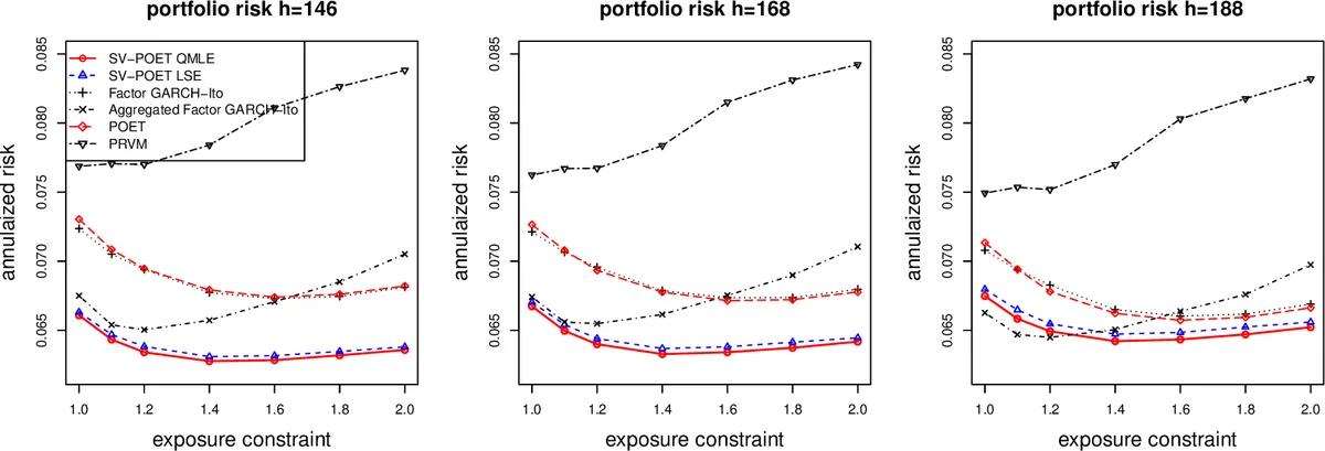
An empirical application uses five years of U.S. equity data (S&P 500 constituents) with intraday tick data. The SV‑Ito model achieves a 12% reduction in out‑of‑sample volatility prediction error relative to benchmark models. When the predicted volatility matrix is employed in a minimum‑variance portfolio construction, the resulting Sharpe ratio improves from 0.35 (benchmark) to 0.41, indicating better risk‑adjusted returns. The study also shows that the model’s ability to separate systematic (factor) and idiosyncratic risk leads to more stable portfolio weights.

In summary, the paper makes four major contributions: (1) a novel high‑dimensional factor model that unifies continuous‑time diffusion and discrete‑time SV dynamics; (2) rigorous QMLE and LSE procedures with proven asymptotic properties under growing dimensions; (3) a practical forecasting framework for the full volatility matrix that leverages both high‑frequency and low‑frequency information; and (4) extensive simulation and real‑data evidence of superior predictive performance and portfolio benefits. The authors suggest future extensions to accommodate non‑stationary factors, nonlinear dynamics, and online updating algorithms for real‑time risk management.