On exact solutions, conservation laws and invariant analysis of the generalized Rosenau-Hyman equation

In this paper, the nonlinear Rosenau-Hyman equation with time dependent variable coefficients is considered for investigating its invariant properties, exact solutions and conservation laws. Using Lie classical method, we derive symmetries admitted by considered equation. Symmetry reductions are performed for each components of optimal set. Also nonclassical approach is employed on considered equation to find some additional supplementary symmetries and corresponding symmetry reductions are performed. Later three kinds of exact solutions of considered equation are presented graphically for different parameters. In addition, local conservation laws are constructed for considered equation by multiplier approach.

💡 Research Summary

The paper investigates a generalized Rosenau‑Hyman (RH) equation with time‑dependent coefficients:
u_t + α(t) u u_{xxx} + δ(t) u_x u_{xx} + β(t) u u_x = 0.
Here α(t), β(t) and δ(t) are non‑zero integrable functions of time. The authors apply both the classical Lie symmetry method and the non‑classical (conditional) symmetry approach to uncover the full symmetry structure of the equation, then use these symmetries to reduce the partial differential equation (PDE) to ordinary differential equations (ODEs) and to construct exact solutions. Finally, they derive several families of local conservation laws via the multiplier method, without requiring a Lagrangian formulation.

Classical Lie symmetries.
Starting from the infinitesimal point transformation (x, t, u) → (x + εξ, t + ετ, u + εη), the authors compute the prolonged infinitesimals η^{(t)}, η^{(x)}, … and impose the invariance condition on (1.1). By separating coefficients of linearly independent monomials they obtain a determining system (2.5). Solving it yields τ, ξ and η expressed through α(t) and its antiderivative Rα(t)=∫α^{-1}(t)dt (equations (2.6)–(2.7)). The resulting Lie algebra is spanned by three generators:
V₁ = x∂_x − Rα(t)∂_t + 4u∂_u, V₂ = ∂_x, V₃ = α^{-1}(t)∂_t.
To avoid equivalent reductions the authors construct an optimal system, selecting V₁ and the combination V₂ + λV₃. For each generator they derive similarity variables (ζ) and similarity transformations for u, reducing the PDE to ODEs (2.9) and (2.10). The first reduction leads to a third‑order nonlinear ODE in ζ, while the second yields a second‑order ODE containing the parameter λ.

Non‑classical symmetries.
The conditional symmetry ansatz u_t = ξ(x,t,u) u_x + η(x,t,u) is substituted into (1.1). By eliminating u_t and the highest derivative u_{xxx} using the ansatz, a set of nonlinear determining equations (3.4) is obtained. Solving these gives ξ = f(t)(x + c₁), η = c₂ f(t) u, where f(t) is an arbitrary integrable function and c₁, c₂ are constants. The associated infinitesimal generator is X = f(t)(x + c₁)∂_x + ∂_t + c₂ u f(t)∂_u. Integrating the characteristic system yields the similarity variable z = (x + c₁) exp(−∫f(t)dt) and the reduced dependent variable u = exp(c₂∫f(t)dt) g(z). Substitution reduces the original PDE to the ODE (3.9), a third‑order nonlinear equation in g(z).

Exact solutions.
For the ODE (2.9) the authors assume a quadratic polynomial f(ζ)=a+bζ+cζ². Coefficient comparison forces a = 0, b = −3c₅, c = 0, giving the explicit solution
u(x,t) = −3c₅ x exp(−∫α(t)dt).
They present three‑dimensional and contour plots for several choices of α(t) (e^{-t}, sinh t, ln t) and different values of c₅, illustrating how the solution profile changes with the time‑dependent coefficient.

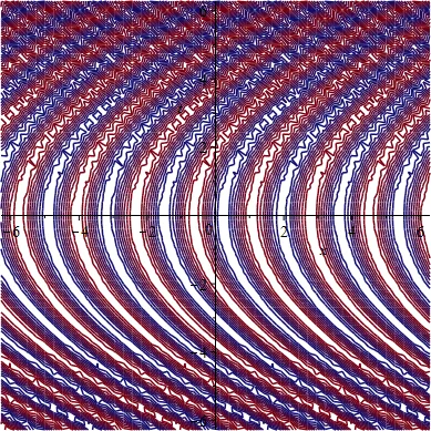
For the ODE (2.10) they set λ = 1 (the general case is left for future work) and integrate once to obtain a second‑order equation. Using Maple they find a trigonometric solution:
f(ζ) = c₁ sin(ζ/(√2 λ √c₅)) + c₂ cos(ζ/(√2 λ √c₅)) + 2c₅ λ³.
Consequently the original PDE admits the wave‑like solution (4.7), which is again visualized for various parameter sets (α(t)=1, α(t)=t, different λ and c₅).

For the non‑classical reduction (3.9) a quadratic ansatz g(z)=a+bz+cz² leads to a simple solution
u(x,t) = 1 − (c₂/c₄)(x + c₁) exp(∫(c₂−1)f(t)dt).
Again, a series of 3‑D and contour plots are provided for exponential, sinusoidal and tangent choices of f(t).

Conservation laws via multipliers.
The multiplier method assumes a scalar multiplier Λ(x,t,u) such that Λ·(PDE) becomes a total divergence D_t C^t + D_x C^x. Applying the Euler operator yields the determining equations (5.5). The authors split the analysis according to algebraic relations among α, β and δ, leading to four main cases (a)–(d) and several sub‑cases. For each they present explicit multipliers (e.g., constant Λ, Λ=c₁+c₂ u^{c₃−1}, Λ=c₂ ln u + c₁, etc.) and the corresponding conserved densities C^t and fluxes C^x. Notably, when α=β=1 and δ=3 (the original RH equation) the derived conservation laws coincide with those known in the literature, confirming the correctness of the approach. In other parameter regimes the paper uncovers new families of conserved vectors, some involving sinusoidal or exponential spatial dependence.

Conclusions.
The study demonstrates that the generalized RH equation with time‑dependent coefficients possesses a rich symmetry structure. Classical Lie symmetries provide a systematic reduction to ODEs and yield explicit polynomial and trigonometric solutions. The non‑classical (conditional) symmetry analysis uncovers additional reductions not accessible by the classical method, leading to further exact solutions. The multiplier technique furnishes several local conservation laws without requiring a variational formulation, and the results specialize correctly to the constant‑coefficient RH equation. The authors argue that the flexibility introduced by variable coefficients makes the model more suitable for describing physical phenomena where material properties or external forces change in time (e.g., pattern formation in liquid drops). They suggest future work on higher‑dimensional extensions, more general coefficient functions, and numerical validation of the analytical solutions.