Temporal mixture ensemble models for intraday volume forecasting in cryptocurrency exchange markets

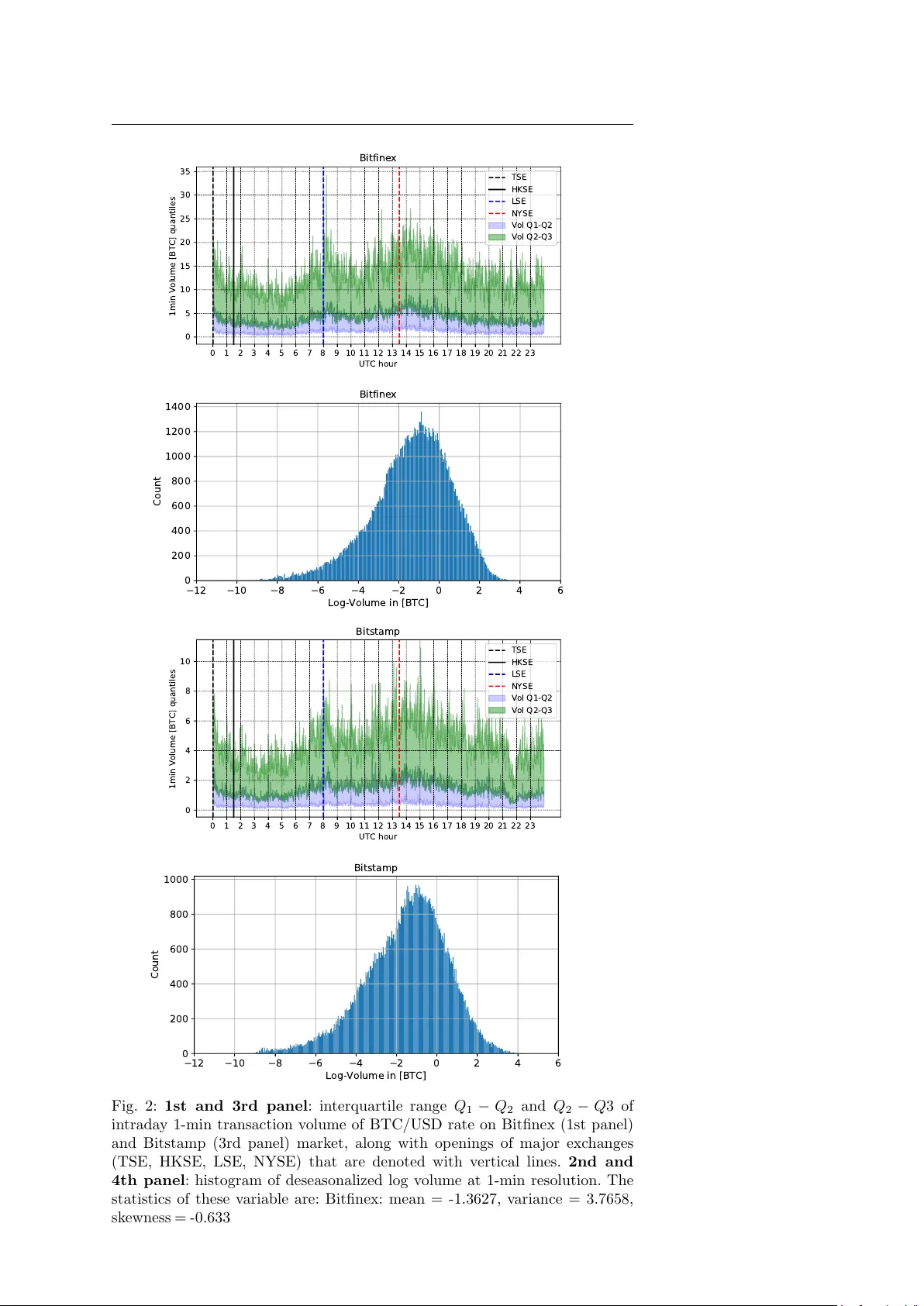
Noname man uscript No. (will b e inserted b y the editor) T emp oral mixture ensem ble for probabilistic forecasting of intrada y volume in crypto currency exchange mark ets Nino Antulo v-F an tulin* · Tian Guo* · F abrizio Lillo Received: date / Accepted: date Abstract W e study the problem of the in traday short-term volume forecast- ing in crypto currency exc hange mark ets. The predictions are built by using transaction and order b o ok data from different mark ets where the exchange tak es place. Metho dologically , w e prop ose a temp oral mixture ensemble, ca- pable of adaptively exploiting, for the forecasting, different sources of data and providing a v olume p oint estimate, as w ell as its uncertaint y . W e provide evidence of the outp erformance of our mo del b y comparing its outcomes with those obtained with different time series and machine learning metho ds. Fi- nally , we discuss the predictions conditional to v olume and we find that also in this case mac hine learning metho ds outp erform econometric mo dels. 1 In tro duction Crypto currencies recently attracted massiv e attention from public and re- searc her communit y in sev eral disciplines such as finance and economics [1 – 6], computer science [7 – 11] or complex systems [12 – 17]. It originated from a de- cen tralized peer-to-p eer paymen t netw ork [18], relying on cryptographic meth- o ds [19, 20] like elliptical curve cryptography and the SHA-256 hash function. *Shared first authorship. N. An tulov-F an tulin ETH Zuric h Aisot Gm bH, Zuric h, Switzerland T. Guo RAM Activ e In vestmen ts, Switzerland W ork done when at ETH Zurich F. Lillo Department of Mathematics,Universit y of Bologna Scuola Normale Sup eriore, Pisa, Italy E-mail: fabrizio.lillo@unib o.it 2 Nino Antulo v-F antulin* et al. When new transactions are announced on this net work, they ha ve to be v er- ified b y net w ork nodes and recorded in a public distributed ledger called the blo c kc hain [18]. Crypto currencies are created as a reward in the verification comp etition (see Pro of of w ork [21]), in which users offer their computing p o wer to v erify and record transactions in to the block chain. Bitcoin is one of the most prominen t decen tralized digital cryptocurrencies and it is the fo cus of this pap er, although the model developed b elow can be adapted to other cryp- to currencies with ease, as w ell as to other ”ordinary” assets (equities, futures, FX rates, etc.). The exc hange of Bitcoins with other fiat or crypto currencies takes place on exc hange markets, which share some similarities with the foreign exchange mark ets [22]. These markets typically work through a contin uous double auc- tion, which is implemen ted with a limit order b o ok mec hanism, where no designated dealer or market maker is presen t and limit and market orders to buy and sell arrive contin uously . Moreov er, as observed for traditional assets, the market is fr agmente d , i.e. there are several exchanges where the trading of the same asset, in our case the exchange of a crypto currency with a fiat currency , can simultaneously take place. Fig. 1: Illustration of the probabilistic volume predicting in the m ulti-source data setting of Bitfinex and Bitstamp markets. The left and right panel re- sp ectiv ely depict the order b o ok and transaction data of eac h market. The arro ws represent the data used to mo del the volume of eac h market. Note that the volume information is implicitly con tained in the transaction data of one mark et and thus there is no arrow linking the volumes from the tw o markets. The automation of the (crypto currency) exchanges lead to the increase of the use of automated trading [23, 24] via different trading algorithms. An im- p ortan t input for these algos is the prediction of future trading volume. This is imp ortant for several reasons. First, trading volume is a proxy for liquidit y whic h in turn is important to quan tify transaction costs. T rading algorithms aim at minimizing these costs by splitting orders in order to find a b etter exe- cution price [25, 26] and the crucial part is the decision of when to execute the orders in such a wa y to minimize market impact or to achiev e certain trading b enc hmarks (e.g. VW AP) [27 – 32]. Second, when differen t market ven ues are a v ailable, the algorithm must decide where to p ost the order and the c hoice is likely the market where more volume is predicted to b e av ailable. Third, T emporal mixture ensemble for cryptocurrency intrada y volume forecasting 3 v olume is also used to mo del the time-v arying price v olatilit y process, whose relation is also kno wn as “Mixture of Distribution Hyp othesis” [33]. In this pap er, w e study the problem of in trada y short-term volume pre- diction on multi-mark et of crypto currency , as is shown in Fig. 1, intending to obtain not only point estimate but also the uncertain ty on the p oint predic- tion [1, 4, 34, 35]. Moreo ver, conv entional volume predictions focuses on using data or features from the same mark et. Since crypto currency markets are traded on several markets simultaneously , it is reasonable to use cross-market data not only to enhance the predictiv e p ow er, but also to help understanding the interaction b etw een markets. In particular, we inv estigate the exc hange rate of Bitcoin (BTC) with a fiat currency (USD) on tw o liquid mark ets: Bitfinex and Bitstamp. The first market is more liquid than the second, since its traded v olume in the in vestigated perio d from June 2018 to No vem b er 2018 is 2 . 5 times larger 1 . Thus one expects an asymmetric role of the past v olume (or other mark et v ariables) of one market on the prediction of v olume in the other mark et. Sp ecifically , the contribution of this pap er can b e summarized as follows: – W e formulate the cross-market volume prediction as a sup ervised m ulti- source learning problem. W e use m ulti-source data, i.e. transactions and limit order bo oks from differen t mark ets, to predict the v olume of the target mark et. – W e prop ose the T emp oral M ixture E nsemble (TME), which mo dels indi- vidual source’s relation to the target and adaptively adjusts the contribu- tion of the individual source to the target prediction. – By equipping with mo dern ensemble techniques, the prop osed mo del can further quantify the predictive uncertaint y consisting of the epistemic and aleatoric comp onen ts, on the predicted volume. – As main benchmarks for v olume dynamics, we use differen t time-series and mac hine learning models (clearly with the same regressors/features used in our model). W e observ e that our dynamic mixture ensem ble is often ha ving sup erior out-of-sample performance on con ven tional prediction error met- rics e.g. ro ot mean square error (RMSE) and mean absolute error (MAE). More imp ortantly , it presents m uc h b etter calibrated results, ev aluated by metrics taking in to accoun t predictiv e uncertain ty , i.e. normalized negativ e log-lik eliho o d (NNLL), uncertaint y interv al width (IW). – W e discuss the prediction p erformance conditional to v olume. Since our c hoice of modeling log-volume is tan tamount to considering a multiplica- tiv e noise mo del for volumes, when using relative RMSE and MAE machine learning metho ds outp erforms econometric mo dels in providing more ac- curate forecasts. 1 Recently , there hav e been few rep orts that are showing fake reported volume for certain Bitcoin exchange markets. In this pap er, we inv estigate Bitcoin exchange markets that hav e regulatory status [36] either with the Money Services Business (MSB) license or BitLicense from the New Y ork State Department of Financial Services, and hav e b een indep endently verified to report true v alues. 4 Nino Antulo v-F antulin* et al. The paper is organized as follows: in Sec. 2 w e presen t the in vestigated mark ets, the data, and the v ariables used in the modeling. In Sec. 3 w e present our b enchmark mo dels. In Sec. 4 we present our empirical in vestigations on the crypto currency markets for the prediction of intrada y market v olume. Finally , Sec. 5 presen ts some conclusions and outlo ok for future work. Most of the tec hnical description of mo dels and algorithms, as well as some additional empirical results, are presen ted in an app endix. 2 Multiple mark et crypto currency data Our empirical analyses are p erformed on a sample of data o v er the perio d from May 31, 2018 9:55pm (UTC) until Sp etember 30 2018 9:59pm (UTC) from t wo exchange markets, Bitfinex 2 and Bitstamp 3 , where Bitcoins can b e exc hanged with US dollars. These mark ets w ork through a limit order b o ok, as many conv en tional exchanges. F or each of the tw o markets we consider tw o t yp es of data: transaction data and limit order b o ok data. F rom transaction data w e extract the following features on each 1-min in terv al: – Buy volume - num b er of BTCs traded in buy er initiated transactions – Sel l volume - num b er of BTCs traded in seller initiated transactions – V olume imb alanc e - absolute difference b etw een buy and sell volume – Buy tr ansactions - num b er of executed transactions on buy side – Sel l tr ansactions - num b er of executed tr ansactions on sell side – T r ansaction imb alanc e - absolute difference betw een buy and sell num b er of transactions W e remind that a buyer (seller) initiated transaction in a limit order b o ok mark et is a trade where the initiator is a buy (sell) market order or a buy (sell) limit order crossing the spread. F rom limit order b o ok data we extract the following features eac h min ute [37, 38]: – Spr e ad is the difference b etw een the highest price that a buyer is willing to pa y for a BTC (bid) and the lo west price that a seller is willing to accept (ask). – Ask volume is the n umber of BTCs on the ask side of order b o ok. – Bid volume is the n umber of BTCs on the bid side of order b o ok. – Imb alanc e is the absolute difference b etw een ask and bid v olume. – Ask/bid Slop e is estimated as the volume until δ price offset from the b est ask/bid price. δ is estimated by the bid price at the order that has at least 1%, 5% and 10 % of orders with the highest bid price. 2 https://www.bitfinex.com 3 https://www.bitstamp.net T emporal mixture ensemble for cryptocurrency intrada y volume forecasting 5 – Slop e imb alanc e is the absolute difference b etw een ask and bid slop e at differen t v alues of price associated to δ . δ is estimated b y the bid price at the order that has at least 1%, 5% and 10 % of orders with the highest bid price. The target v ariable that w e aim at forecasting is the trading volume of a given target market including b oth buy and sell v olume. In the prop osed mo deling approac hes (describ ed in Sec. 3) we consider different data sources at eac h time can affect the probabilit y distribution of trading volume in the next time interv al in a giv en market. As is illustrated in Fig. 1, giv en the setting presented ab ov e, there are four sources, namely one for transaction data and one for limit order b o ok data for the tw o markets. Before going in to the details of models, in order to c ho ose the appropriated v ariable to inv estigate, we visualize some characteristics of the data in Fig. 2. In the 1st and 3rd panel, we sho w the quan tiles of in trada y 1-min trading v olume of BTC/USD rates, for the t w o differen t mark ets. W e also show as v ertical lines the op ening times of four ma jor sto c k exchanges. Although w e do not observe abrupt changes in volume distribution (p ossibly b ecause cryp- to currency exchanges are weakly related with sto ck exchanges), some small but significan t intrada y pattern [39] is observed. F or this reason, we pre-pro cess the raw v olume data to remov e intrada y patterns as follows. Let us denote v t the volume traded at the time t , in units of Bitcoins. I ( t ) is a mapping function of the time t , whic h returns the in traday time in terv al index of t . W e use a I ( t ) to represen t the a v erage of v olumes at the same in traday index I ( t ) across da ys. Next, to remov e intrada y patterns, w e pro cess the ra w v olume by taking as modeled v ariable y t , v t a I ( t ) . In practise, in order to a void leaking information to the training phase, a I ( t ) is calculated only based on the training data, and shared to b oth v alidating and testing data. The histogram of log y t for the tw o markets 4 is shown in the 2nd and 4th panel of Fig. 2 along with first four cumulan ts of empirical distribution of log-v olumes. W e observ e that the distribution is approximately normal, ev en if a small negativ e skew is presen t. F or this reason, as done in the literature (see for example [40], our mo deling choice is to consider y t as log-normally distributed. 3 Mo dels Econometric mo deling of in tra-daily trading volume relies on a set of em- pirical regularities [27 – 29] of volume dynamics. These include fat tails, strong p ersistence and an in tra-daily clustering around the ”U”-shaped p erio dic com- p onen t. Brownlees et al. [27] proposed Comp onent Multiplicativ e Error Mo del (CMEM), whic h is the extension of Multiplicativ e Error Model (MEM) [41]. 4 The frequency of time interv als with zero volume and how we handle them is detailed in Section 2. 6 Nino Antulo v-F antulin* et al. 0 1 2 3 4 5 6 7 8 9 10 11 12 13 14 15 16 17 18 19 20 21 22 23 UTC hour 0 5 10 15 20 25 30 35 1min Volume [BTC] quantiles Bitfinex TSE HKSE LSE NYSE Vol Q1-Q2 Vol Q2-Q3 12 10 8 6 4 2 0 2 4 6 Log-Volume in [BTC] 0 200 400 600 800 1000 1200 1400 Count Bitfinex 0 1 2 3 4 5 6 7 8 9 10 11 12 13 14 15 16 17 18 19 20 21 22 23 UTC hour 0 2 4 6 8 10 1min Volume [BTC] quantiles Bitstamp TSE HKSE LSE NYSE Vol Q1-Q2 Vol Q2-Q3 12 10 8 6 4 2 0 2 4 6 Log-Volume in [BTC] 0 200 400 600 800 1000 Count Bitstamp Fig. 2: 1st and 3rd panel : interquartile range Q 1 − Q 2 and Q 2 − Q 3 of in traday 1-min transaction v olume of BTC/USD rate on Bitfinex (1st panel) and Bitstamp (3rd panel) market, along with op enings of ma jor exchanges (TSE, HKSE, LSE, NYSE) that are denoted with vertical lines. 2nd and 4th panel : histogram of deseasonalized log volume at 1-min resolution. The statistics of these v ariable are: Bitfinex: mean = -1.3627, v ariance = 3.7658, sk ewness = -0.6336, and kurtosis = 0.6886; Bitstamp: mean = -2.4224, v ariance = 3.9894, sk ewness = -0.5307, kurtosis = 0.4114. T emporal mixture ensemble for cryptocurrency intrada y volume forecasting 7 The CMEM v olume mo del has a connection to the component-GAR CH [42] and the perio dic P-GAR CH [43]. Satish et al. [28], proposed four-component v olume forecast model composed of: (i) rolling historical volume av erage, (ii) daily ARMA for serial correlation across daily volumes, (iii) deseasonalized in tra-day ARMA v olume mo del and (iv) a dynamic w eigh ted combination of previous mo dels. Chen et al. [29], simplify the multiplicativ e v olume model [27] in to an additiv e one b y mo deling the logarithm of in traday v olume with the Kalman filter. 3.1 Problem setting In this pap er, we focus on the probabilistic forecasting including b oth mean and v ariance of the intrada y v olume in the multi-source data setting. W e pro- p ose the use of TME, presented b elow, and we b enchmark its p erformance against tw o econometric baseline mo dels (ARMA-GARCH and ARMAX-GAR CH) and one Mac hine Learning baseline mo del (Gradient Bo osting Machine). As men tioned ab o ve, we assume y t follo ws the log-normal distribution [40] and thus all the mo dels used in the exp eriments will b e developed to learn the log-normal distribution of y t . How ever, our prop osed TME is flexible to b e equipped with differen t distributions for the target, and the study in this direction will b e the future w ork. When ev aluating the p erformance of the forecasting pro cedure with real data exp eriments, we c ho ose to use ev aluation metrics defined on the original v olume v t , since in real world application the interest is in forecasting volume rather than log-volume. Finally , for understanding the p erformance of TME and Mac hine Learning and econometric baselines in different setups, w e will ev aluate them using three different time interv als of volumes, namely 1min, 5min and 10min. Regarding the multi-source data setting, on one hand, it includes the fea- tures from the target mark et. This data is b elieved to be directly correlated with the target v ariable. On the other hand, there is an alternative market, whic h could interact with the target market. T ogether with the target market, the features from this alternativ e market constitute the multi-source data. In this pap er, we mainly fo cus on Bitfinex and Bitstamp markets. F or eac h market, w e ha ve the features from b oth transaction and order b o ok data, thereb y leading to S = 4 data sources. In particular, we indicate with x s,t ∈ R d s the features from source s at time step t , and d s the dimensionality of source data s . Giv en the list of features presen ted in Sec. 2, we ha ve d s = 6 when the source is transaction data in any market, while d s = 13 for order b o ok data. Then, these multi-source data will b e used to mo del the volume of eac h market, as is shown in Fig. 1. 8 Nino Antulo v-F antulin* et al. 3.2 Ov erview of TME In this pap er, we construct a T emp oral Mixture Ensemble (TME), belonging to the class of of mixture mo dels [44 – 48], which takes previous transactions and limit order b o ok data [37, 38] from m ultiple markets simultaneously into accoun t. Though mixture mo dels ha ve b een widely used in mac hine learning and deep learning [11, 49, 50], they hav e b een hardly explored for prediction tasks in crypto currency markets. Moreov er, our proposed ensemble of temp oral mixtures can provide predictiv e uncertaint y of the target volume b y the use of the Stochastic Gradient Descent (SGD) based ensemble technique [51 – 53]. Predictiv e uncertaint y reflects the confidence of the mo del o ver the prediction. It is v aluable extra information for mo del interpretabilit y and reliability . The mo del developed b elow is flexible to consume multi-source data of arbitrary n umber of sources and dimensionalities of individual source data. In principle, TME exploits latent v ariables to capture the contributions of differen t sources of data to the future evolution of the target v ariable. The source contributing at a certain time dep ends on the history of all the sources. F or simplicity , w e will use one data sample of the target y t to present the prop osed model. In realit y , the training, v alidation, and testing data con tain the samples collected in a time perio d. More quantitativ ely , the generativ e pro- cess of the target v ariable y t conditional on multi-source data { x 1 ,t , · · · , x S,t } is form ulated as the following probabilistic mixture pro cess: p ( y t |{ x 1 , µ,s · x s, ( − h,t ) · R µ,s + b µ,s (4) σ 2 t,s , exp( L > σ,s · x s, ( − h,t ) · R σ,s + b σ,s ) , (5) where L µ,s , L σ,s ∈ R d s and R µ,s , R σ,s ∈ R h . b µ,s , while b σ,s ∈ R are bias terms. Note that the abov e parameters are data source specific and then the trainable set of parameters is denoted b y θ s , { L µ,s , L σ,s , R µ,s , R σ,s , b µ,s , b σ,s } . Based on the prop erties of log-normal distribution [54, 55], the mean and v ariance of the volume target on the original scale mo deled by individual data sources can b e deriv ed from the mean and v ariance of log transformed volume as: E [ y t | z t = s, x s, ( − h,t ) , θ s ] = exp { µ t,s + 1 2 · σ 2 t,s } (6) and V [ y t | z t = s, x s, ( − h,t ) , θ s ] = exp { σ 2 t,s − 1 } · exp { 2 · µ t,s + σ 2 t,s } (7) Then, we define the probability distribution of the latent v ariable z t using a softmax function as follo ws: P ω ( z t = s | x 1 , ( − h,t ) , · · · , x S, ( − h,t ) ) , exp( f s ( x s, ( − h,t ) ) ) exp( P S k =1 f k ( x k, ( − h,t ) ) ) , (8) where f s ( x s, ( − h,t ) ) , L > z ,s · x s, ( − h,t ) · R z ,s + b z ,s (9) 10 Nino Antulo v-F antulin* et al. ω , { L z ,s , R z ,s , b z ,s } S s =1 denotes the set of trainable parameters regarding the laten t v ariable z t , i.e. L z ,s , R z ,s ∈ R d s and b z ,s ∈ R is a bias term. In the following, we will present how the distributions mo deled b y individ- ual data sources and the laten t v ariable will be used to learn the parameters in the training phase and to predict the mean and v ariance of the target v olume in the predicting phase. 3.4 Learning The learning pro cess of TME is based on SGD optimization [56, 57]. It is able to giv e rise to a set of parameter realizations for building the ensemble whic h has b een pro v en to be an effective tec hnique for enhancing the prediction accuracy as w ell as enabling uncertaint y estimation in previous works [51, 52]. W e first briefly describ e the training pro cess of SGD optimization. Denote the set of the parameters by Θ , { θ 1 , · · · , θ S , ω } . The whole training dataset denoted by D is consisted of data instances, eac h of whic h is a pair of y t and { x s, ( − h,t ) } S 1 . t is a time instan t in the p erio d { 1 , · · · , T } . Starting from a random initialized v alue of Θ , in each iteration SGD sam- ples a batc h of training instances to up date the mo del parameters as follows: Θ ( i ) = Θ ( i − 1) − η ∇L ( Θ ( i − 1); D i ) , (10) where i is the iteration step, Θ ( i ) represen ts the v alues of Θ at step i , i.e. a snapshot of Θ . η is the learning rate, a tunable hyperparameter to con trol the magnitude of gradient up date. ∇L ( Θ ( i − 1); D i ) is the gradient of the loss function w.r.t. the model parameters given data batc h D i at iteration i . The iteration stops when the loss conv erges with negligible v ariation. The mo del parameter snapshot at the last step or with the best v alidation p erformance will b e tak en as one realization of the mo del parameters. The learning pro cess of TME is to minimize the loss function defined b y the negativ e log likelihoo d of the target volume as: L ( Θ ; D ) , − T X t =1 ln S X z t =1 p θ s ( y t | z t = s, x s, ( − h,t ) ) · P ω ( z t = s |{ x s, ( − h,t ) } S 1 ) − log p ( Θ ) , (11) where the prior p ( Θ ) is view ed as a regularisation term. By plugging the probability density function of log-normal distribution and Gaussian prior of Θ as a L2 regularisation, Eq. 11 is further expressed as: − T X t =1 ln S X z t =1 1 y t σ t,s √ 2 π exp  − (ln y t − µ t,s ) 2 2 σ 2 t,s  · P ω ( z t = s |{ x s, ( − h,t ) } S 1 ) − λ k Θ k 2 2 , (12) T emporal mixture ensemble for cryptocurrency intrada y volume forecasting 11 where λ is the h yp er-parameter of regularization strength. In the SGD optimization pro cess, different initialization of Θ leads to dis- tinct parameter iterate tra jectories. Recent studies sho w that the ensemble of indep endently initialized and trained mo del parameters empirically often pro vide comparable p erformance on uncertain ty quantification w.r.t. sam- pling and v ariational inference based metho ds [51 – 53]. Our ensem ble construc- tion follows this idea b y taking a set of model parameter realizations from differen t training tra jectories, and each parameter realization is denoted by Θ m = { θ m, 1 , · · · , θ m,S , ω m } . F or more algorithmic details ab out the collecting pro cedure of these parameter realizations, please refer to the app endix. 3.5 Prediction In this part, we present the predicting pro cess given mo del parameter realiza- tions { Θ m } M 1 . W e fo cus on t wo t yp es of prediction quan tities, i.e. mean and v ariance. Sp ecifically , the predictiv e mean of the target in the original scale is defined as: E [ y t |{ x s, ( − h,t ) } S s =1 , D ] ≈ 1 M M X m =1 E [ y t | { x s, ( − h,t ) } S s =1 , Θ m ] , (13) where E [ y t |{ x s, ( − h,t ) } S s =1 , Θ m ] is the conditional mean given one realization Θ m . In TME, it is a weigh ted sum of the predictions by individual data sources as: E [ y t |{ x s, ( − h,t ) } S s =1 , Θ m ] = S X s =1 P ω m ( z t = s |{ x s, ( − h,t ) } S s =1 ) · E [ y t | z t = s, x s, ( − h,t ) , θ m,s ] (14) Apart from the predictive mean, the predictive v ariance is of great interest as well, since it helps to quantify the uncertain ty on the prediction, thereby facilitating the downstream decision making based on the volume predictions. Giv en the predictive mean, eac h data source’s mean and v ariance defined in Eq. 6, 7 and 13, the predictiv e v ariance of the target volume is derived as: V ( y t |{ x s, ( − h,t ) } S s =1 , D ) ≈ Z y y 2 p ( y |{ x s, ( − h,t ) } s , D ) dy − E 2 [ y t |{ x s, ( − h,t ) } S s =1 , D ] = 1 M M X m =1 S X s =1 P ω m ( z t = s |· ) V ( y t | z t = s, x s, ( − h,t ) , θ m,s ) | {z } Aleatoric Uncertain ty + 1 M M X m =1 S X s =1 P ω m ( z t = s |· ) E 2 [ y t | z t = s, x s, ( − h,t ) , θ m,s ) − E 2 [ y t |{ x s, ( − h,t ) } S s =1 , D ] , | {z } Epistemic Uncertain ty (15) 12 Nino Antulo v-F antulin* et al. where for clarity of the formula P ω m ( z t = s |{ x s, ( − h,t ) } S s =1 ) is simplified to P ω m ( z t = s |· ). Eq. 15 sho ws that the predictive v ariance is comp osed of tw o types of un- certain ties, aleatoric and epistemic uncertaint y . The aleatoric part in Eq. 15 stems from v ariance induced from multi-source data. It captures the noise inheren t to the target which could depend on x s, ( − h,t ) . As a comparison, the classical aleatoric uncertain t y (or v olatility) estimation model is typically used to estimate the uncertaint y solely with the target time series or external fea- tures as a whole. It has no mec hanism to capture the evolving relev ance of m ulti-source data to the aleatoric uncertaint y of the target. The epistemic un- certain ty part in Eq. 15 accounts for uncertaint y in the mo del parameters i.e. uncertain ty whic h captures our ignorance ab out which mo del generated our collected data. It is also referred to as the mo del uncertaint y . 4 Exp erimen ts In this section, w e report the ov erall exp erimental ev aluation. More detailed results are in the app endix section. 4.1 Data and metrics Data : W e collected the limit order b o ok and transaction data resp ectively from tw o exchanges, Bitfinex and Bitstamp and extracted features defined in Sec. 2 from the order bo ok and transactions of each exchange for the perio d from Ma y 31, 2018 9:55pm (UTC) until Septem b er 30, 2018 9:59pm (UTC). Then, for eac h exchange, we build three datasets of differen t prediction hori- zons, i.e. 1min, 5min, 10min, for training and ev aluating models. Dep ending on the prediction horizon, eac h instance in the dataset contains a target vol- ume and the time-lagged features from order b o ok and transactions of tw o exc hanges. In particular, for Bitfinex, the sizes of datasets for 1min, 5min, 10min are resp ectively 171727, 34346 and 17171. F or Bitstamp, the sizes of datasets are respectively 168743, 33749 and 16873. In all the exp erimen ts, data instances are time ordered and we use the first 70% of p oints for training, the next 10% for v alidation, and the last 20% of p oints for out-of-sample testing. Note that all the metrics are ev aluated on the out of sample testing data. F or modeling the log-normal distribution, the baseline mo dels and TME need to p erform the log-transformation on y t and thus in the data pre-pro cessing step, we ha v e filtered out the data instances with zero trading volume. Em- pirically , we found out that these zero-v olume data instances account for less than 2 . 25% and 3 . 98% of the entire dataset for Bitfinex and Bitstamp mark ets resp ectiv ely . F or the baseline metho ds not differentiating the data source of features, eac h target v olume has a feature v ector built b y concatenating all features from order b o ok and transactions of tw o markets into one v ector. F or our TME, T emporal mixture ensemble for cryptocurrency intrada y volume forecasting 13 eac h target v olume has four groups of features resp ectively corresp onding to the order b o ok and transaction data of t wo markets. Metrics : Note that baseline mo dels and TME are trained to learn the log- normal distribution of the deseasonalized volume, how ever, the following met- rics are ev aluated on the original scale of the volume, b ecause our aim is to quan tify the p erformance on the real volume scale, that is of more interest for practical purp oses. In the following definitions, ˆ v t corresp onds to the predictive mean of the ra w volume. T is the num b er of data instances in the testing dataset. ˆ v t is deriv ed from the predictive mean of y t m ultiplied by a I ( t ) , according to the definition of y t in Sec. 3. F or baseline mo dels, the predictive mean of y t is deriv ed from the mean of logarithmic transformed y t via Eq. 6 used by indi- vidual sources in TME. The predictiv e mean of y t b y TME is shown in Eq.13. The considered p erformance metrics are: RMSE: is the ro ot mean square error as RMSE = q 1 T P T t =1 ( v t − ˆ v t ) 2 . MAE: is mean absolute error as MAE = 1 T P T t =1 | v t − ˆ v t | . NNLL: is the predictive Negative Log-Likelihoo d of testing instances nor- malized b y the total n umber of testing p oints. F or the target v ariable volume, the likelihoo d of the real v t is that of the corresp onding intrada y-pattern free y t scaled b y 1 a I ( t ) , according to the definition in Sec.3. F or TME, the lik eliho o d of y t is calculated, as shown in Eq. 12, based on the mixture of log-normal dis- tributions taking in to account b oth predictiv e mean and v ariance. F or baseline mo dels, the likelihoo d of y t can b e straightforw ardly derived from the predic- tiv e mean and v ariance of ln y t [54, 55]. IW: interv al width is meant to ev aluate the uncertaint y around the p oint prediction, i.e. predictive mean, in probabilistic forecasting. The ideal mo del is exp ected to provide tigh t interv als, which imply the model is confiden t in the prediction. In this pap er, our baseline mo dels and TME inv olve unimo dal and multimodal distributions, i.e. log-normal and mixture of log-normal. As a result, we c ho ose to measure the interv al width simply using the v ariance [58]. Sp ecifically , IW is defined as the a veraged standard deviation of the testing instances. Note that similar to the scaling op eration for getting ˆ v t , the standard deviation is obtained via firstly scaling the predictiv e v ariance of y t b y a 2 I ( t ) . 4.2 Baseline mo dels and TME setup As mentioned abov e, we benchmark the p erformance of TME against t wo econometric and one Mac hine Learning mo dels. W e present them b elow. ARMA-GAR CH is the autoregressive moving av erage mo del (ARMA) plus generalized autoregressive conditional heterosk edasticity (GAR CH) mo del [27– 29]. It is aimed to resp ectively capture the conditional mean and conditional v ariance of the logarithmic volume. Then, the predictive mean and v ariance of the logarithmic volume are transformed to the original scale of the v olume for ev aluation. 14 Nino Antulo v-F antulin* et al. The n um b er of autoregressiv e and moving av erage lags in ARMA are se- lected in the range from 1 to 10, by minimization of Ak aik e Information Cri- terion, while the orders of lag v ariances and lag residual errors in GARCH are found to affect the p erformance negligibly and thus are b oth fixed to one [59]. The residual diagnostics for ARMA-GARCH mo dels is given in the app endix Figure 5 and Figure 6. In T able 1 we rep ort the estimated GAR CH parameters in the ARMA- GAR CH mo del on the log-volume, together with the standard errors and the p-v alue. All parameters are statistically differen t from zero at all time scales, indicating the significan t existence of heteroskedasticit y . T able 1: Statistics of GARCH(1,1) parameters ( ω , α , β ) on log-volume resid- uals, trained with ARMA( p, q )-GARCH(1,1) mo del for differen t markets and prediction horizons. (*) indicate p-v alues < 10 − 5 for estimated parameters. P arameters p, q , w ere selected b y minimizing AIC and are rep orted in T ables 2-4. BITFINEX ω Std.Err( ω ) α Std.Err( α ) β Std.Err( β ) 1 min 0.0177* 0.0011 0.0259* 0.0008 0.9677* 0.0000 5 min 0.0119* 0.0015 0.0218* 0.0017 0.9663* 0.0000 10 min 0.0062* 0.0011 0.0152* 0.0018 0.9762* 0.0000 BITST AMP ω Std.Err( ω ) α Std.Err( α ) β Std.Err( β ) 1 min 0.0112* 0.0007 0.0203* 0.0006 0.9759* 0.0000 5 min 0.0175* 0.0023 0.0277* 0.0022 0.9561* 0.0000 10 min 0.0262* 0.0056 0.0291* 0.0042 0.9387* 0.0000 ARMAX-GAR CH is the v ariant of ARMA-GARCH b y adding external feature terms. In our scenario, external features are obtained by concatenating all features from order b o ok and transaction data of t w o exc hanges in to one feature vector. The hyper-parameters in ARMAX-GAR CH are selected in the same w ay as for ARMA-GARCH. GBM is the gradient bo osting machine [60]. It has been empirically prov en to b e highly effectiv e in predictiv e tasks across different machine learning c hal- lenges [61, 62] and more recently in finance [63, 64]. The feature v ector fed into GBM is also the concatenation of features from order b o ok and transaction data of tw o markets. The h yp er-parameters [65] of GBM are selected by ran- dom search in the ranges: n umber of trees in [100 , · · · , 1000], max num b er of features used b y individual trees in [1 . 0 , · · · , 0 . 1], minim um n umber of samples of the leaf no des in [2 , · · · , 9], maximum depth of individual trees in [4 , · · · , 9], and the learning rate in [0 . 05 , · · · , 0 . 005]. TME is implemented by T ensorFlo w 6 . The hyper-parameters tuned by ran- dom searc h are mainly the learning rate in the range [0 . 0001 , · · · , 0 . 001], batc h size in [10 , · · · , 300], and the l2 regularization term in [0 . 1 , · · · , 5 . 0]. The num- b er of model parameter realizations for building the ensem ble is set to 20. Bey ond this num b er, we found no significant p erformance improv ement. 6 https://gith ub.com/tensorflow/tensorflo w T emporal mixture ensemble for cryptocurrency intrada y volume forecasting 15 4.3 Results In this section, we present the results on the predictions of v olume in b oth mark ets at different time scales. T ables 2, 3, and 4 show the error metrics on the testing data for the tw o markets and the four mo dels. W e observe that in all cases the smallest RMSE is ac hieved b y TME while the smallest MAE is ac hieved b y GBM. Concerning NNLL, in Bitfinex TME outp erforms the other mo dels for 1-min and 5-min cases, while for Bitstamp markets econometirc mo del hav e (slightly) low er v alues. Finally , the smallest IW is alwa ys ac hieved b y TME. The fact that GBM has sup erior p erformance on MAE is somewhat ex- p ected since GBM has b een trained to minimize p oint prediction, while ARMA- GAR CH, ARMAX-GARCH and TME were trained with a maximum likeli- ho o d ob jectiv e. By comparing RMSE and MAE in b oth mark ets, we observ e that for ARMA-GAR CH mo del in Bitfinex, external features and extra information from Bitstamp are low ering MAE and RMSE errors (except on 1min in ter- v al on Bitfinex mark et). In Bitstamp mark et, for ARMAX-GAR CH mo del external features only help on 1-min in terv al prediction. This phenomenon could indicate the one-directional information relev ance across tw o markets. Ho wev er, due to the data source sp ecific comp onents and temp oral adaptiv e w eighting schema, our TME is able to yield more accurate prediction consis- ten tly , compared to ARMA-GARCH. As for NNLL, similar pattern is observed in ARMA-GARCH family , i.e. additional features impair the NNLL p erformance instead, while TME retains comparable p erformance. More imp ortantly , TME has muc h lo w er IW. T o- gether with the low er RMSE, it implies that when TME predicts the mean closer to the observ ation, the predictiv e uncertain t y is also lo w er. Remind that GBM do es not provide probabilistic predictions. Overall w e find that TME outp erforms quite often the baseline b enchmarks, b y providing smaller RMSE and tigh ter interv als. In order to disen tangle the differen t con tributions to TME predictions and, at the same time, understanding wh y choosing different predicting features at eac h time step is imp ortan t, we present in Fig. 3 and Fig. 4 the predictive v olume and uncertaint y of 5-min volume prediction in a sample time p erio d of the testing data for the t wo markets. P anel (a) sho ws how well the TME (p oin twise and in terv al) predictions follo ws the actual data. The TME is able to quantify at each time step the con tribution of each source to the target forecasting. In Panel(b) we show the dynamical contribution scores of the four sources. These scores are simply the a verage of the probabilit y of the latent v ariable v alue corresp onding to each data source, i.e. z t = s . W e notice that the relativ e con tributions v aries with time and w e observ e that the external order bo ok source from the less liquid mark et (Bitstamp) do es not contribute muc h to predictions. On the contrary , in Panel (b) of Fig. 4, where the data for Bitstamp are shown, external order b o ok and external transaction features from the more liquid mark et (Bitfinex) 16 Nino Antulo v-F antulin* et al. T able 2: Results of 1-min volume prediction. The arro w sym b ols indicate the direction of the metrics for b etter mo dels. GBM mo del is not providing un- certain ty and NNLL and IW results are not a v ailable (NA). Results in bold, indicate the minim um errors among mo dels. BITFINEX MARKET RMSE ↓ MAE ↓ NNLL ↓ IW ↓ ARMA(5,5)-GARCH(1,1) 24.547 14.227 2.660 117.348 ARMAX(5,5)-GARCH(1,1) 24.629 14.189 2.664 117.084 GBM 21.026 7.978 NA NA TME 20.142 10.204 2.654 44.344 BITST AMP MARKET RMSE ↓ MAE ↓ NNLL ↓ IW ↓ ARMA(3,3)-GARCH(1,1) 14.587 7.688 1.719 97.618 ARMAX(3,3)-GARCH(1,1) 14.292 7.487 1.719 93.943 GBM 11.740 3.515 NA NA TME 11.378 4.299 1.720 10.295 T able 3: Results of 5-min volume prediction. The arro w sym b ols indicate the direction of the metrics for b etter mo dels. GBM mo del is not providing un- certain ty and NNLL and IW results are not a v ailable (NA). Results in bold, indicate the minim um errors among mo dels. BITFINEX MARKET RMSE ↓ MAE ↓ NNLL ↓ IW ↓ ARMA(3,3)-GARCH(1,1) 64.999 39.909 4.642 82.158 ARMAX(3,3)-GARCH(1,1) 64.456 39.150 4.641 79.852 GBM 64.964 32.888 NA NA TME 63.855 39.527 4.636 68.748 BITST AMP MARKET RMSE ↓ MAE ↓ NNLL ↓ IW ↓ ARMA(5,4)-GARCH(1,1) 38.300 17.606 3.732 34.797 ARMAX(5,4)-GARCH(1,1) 40.273 18.887 3.766 38.250 GBM 39.196 14.714 NA NA TME 38.223 17.287 3.765 29.148 T able 4: Results of 10-min v olume prediction. The arrow symbols in the first line indicate the direction of the metrics for b etter mo dels. GBM mo del is not pro viding uncertaint y and NNLL and IW results are not av ailable (NA) BITFINEX MARKET RMSE ↓ MAE ↓ NNLL ↓ IW ↓ ARMA(3,2)-GARCH(1,1) 112.872 72.505 5.409 124.890 ARMAX(3,2)-GARCH(1,1) 111.987 71.149 5.373 121.346 GBM 110.197 61.506 NA NA TME 109.878 68.382 5.386 114.195 BITST AMP MARKET RMSE ↓ MAE ↓ NNLL ↓ IW ↓ ARMA(3,2)-GARCH(1,1) 66.486 31.942 4.452 51.228 ARMAX(3,2)-GARCH(1,1) 68.067 32.795 4.457 52.780 GBM 67.128 27.719 NA NA TME 66.234 31.460 4.507 49.972 T emporal mixture ensemble for cryptocurrency intrada y volume forecasting 17 pla y a more dominant role. Then, when we further lo ok at the predictions by individual data sources in TME, see Panel(c)-(f ), what w e observe is in line with the pattern of con tribution scores in Panel(b). F or instance, the comp o- nen t mo del in TME resp onsible for the data source from more liquid Bitfinex captures more uncertaint y , thereb y b eing given high con tribution scores in the v olatile p erio d. The addition of the fea tures from the other markets allo ws to shrink the uncertaint y interv als. W e hav e also rep eated these exp eriments for 1-min and 10-min v olume prediction. The results are collected in the figures and tables in the app endix section. Finally , we discuss how well the differen t predictors p erform conditionally to the volume size. T o this end, we compute for eac h model, market, and time in terv al the RMSE and MAE conditional to the v olume quartile. How ev er, finding the suitable metrics to compare forecasting p erformance of a mo del across differen t quartiles is a subtle issue. T ak e for example a linear mo del for the log-v olume. When considering it as a model for (linear) v olume, it is clear that the additiv e noise in the log-volume b ecomes m ultiplicative in linear v olume. Thus the RMSE conditional to v olume b ecomes prop ortional to (or increasing as a p o wer-la w of ) the volume and therefore one exp ects to see RMSE for high quartiles to b e larger than the one for b ottom quartiles. This is exactly what w e observ e in T able 5 for 5 min horizons (for 1 and 10 min, see the app endix) when lo oking at RMSE and MAE. In order to take into account this statistical effect, essentially caused by the choice of mo deling log-volume and presenting ero or metrics for linear vol- ume, in T able 5 we show also r elative error metrics, namely relative ro ot mean squared error (RelRMSE) and mean absolute percentage error (MAPE) con- ditioned to volume quartile. (RelRMSE is defined as q 1 T P T t =1 ( v t − ˆ v t v t ) 2 ), and MAPE is defined as 1 T P T t =1 | v t − ˆ v t v t | .) In this case the scenario changes com- pletely . First, across all models the relativ e error is smaller for top volume quartiles and larger for b ottom quartiles. Esp ecially relative errors for the lo west quartile are large, likely b ecause small v olumes at the denominator cre- ate large fluctuations. Second, and more imp ortant, TME outp erforms mostly in Q4, while GBM is superior in Q1, Q2, and Q £ frequently . The difference b e- t ween models in Q4 is somewhat smaller, while in Q1-Q3 the out-p erformance of mac hine learning methods is up to a factor 2 with respect to econometric metho ds. Th us also when considering large v olumes and considering relative errors, TME and GBM pro vide more accurate predictions. 18 Nino Antulo v-F antulin* et al. Fig. 3: Visualization of TME in a sample p erio d of Bitfinex for 5-min vol- ume predicting. Panel(a): Predictive mean ± tw o times standard deviation (left-truncated at zero) and the volume observ ations. Panel(b): Data source con tribution scores (i.e. av erage of laten t v ariable probabilities) ov er time. P anel(c)-(f ): Eac h data source’s predictiv e mean ± t wo times standard devi- ation (left-truncated at zero). The color of each source’s plot corresp onds to that of the con tribution score in Panel(b). (b est viewed in colors) T emporal mixture ensemble for cryptocurrency intrada y volume forecasting 19 Fig. 4: Visualization of TME in a sample p erio d of Bitstamp for 5-min v ol- ume predicting. Panel(a): Predictive mean ± tw o times standard deviation (left-truncated at zero) and the volume observ ations. Panel(b): Data source con tribution scores (i.e. av erage of laten t v ariable probabilities) ov er time. P anel(c)-(f ): Eac h data source’s predictiv e mean ± t wo times standard devi- ation (left-truncated at zero). The color of each source’s plot corresp onds to that of the con tribution score in Panel(b). (b est viewed in colors) 20 Nino Antulo v-F antulin* et al. T able 5: 5-min volume prediction errors conditional on the quartile of the true v olume v alues. Measures: RMSE Qx – ro ot mean squared error conditioned on x-th quantile, RelRMSE Qx – relativ e ro ot mean squared error conditioned on x-th quantile, MAE Qx – mean av erage error conditioned on x-th quantile, MAPE Qx – mean absolute p ercen tage error conditioned on x-th quantile. BITFINEX MARKET RMSE Q1 RMSE Q2 RMSE Q3 RMSE Q4 ARMA-GARCH 32.862 38.594 43.073 111.660 ARMAX-GARCH 31.939 36.887 41.005 112.020 GBM 17.632 17.332 22.056 125.604 TME 32.200 32.976 35.928 112.280 RelRMSE Q1 RelRMSE Q2 RelRMSE Q3 RelRMSE Q4 ARMA-GARCH 19.417 2.769 1.299 0.609 ARMAX-GARCH 18.845 2.657 1.243 0.594 GBM 12.672 1.268 0.615 0.623 TME 26.235 2.378 1.098 0.578 MAE Q1 MAE Q2 MAE Q3 MAE Q4 ARMA-GARCH 26.781 28.635 29.622 74.576 ARMAX-GARCH 26.145 27.625 28.190 74.612 GBM 14.719 11.985 16.674 88.122 TME 26.317 28.784 23.338 74.484 MAPE Q1 MAPE Q2 MAPE Q3 MAPE Q4 ARMA-GARCH 9.506 2.003 0.871 0.497 ARMAX-GARCH 9.272 1.935 0.831 0.493 GBM 5.717 0.846 0.460 0.570 TME 11.424 1.823 0.690 0.503 BITST AMP MARKET RMSE Q1 RMSE Q2 RMSE Q3 RMSE Q4 ARMA-GARCH 13.465 15.304 16.199 72.046 ARMAX-GARCH 14.2 16.835 20.0009 74.8532 GBM 6.432 6.679 8.732 77.317 TME 13.617 14.492 14.583 73.778 RelRMSE Q1 RelRMSE Q2 RelRMSE Q3 RelRMSE Q4 ARMA-GARCH 22.171 2.563 1.175 0.671 ARMAX-GARCH 24.259 2.784 1.429 0.889 GBM 12.578 1.154 0.596 0.658 TME 29.289 2.429 1.084 0.586 MAE Q1 MAE Q2 MAE Q3 MAE Q4 ARMA-GARCH 10.668 11.648 11.020 37.094 ARMAX-GARCH 11.0917 12.275 12.1831 39.9903 GBM 5.037 4.575 6.705 42.506 TME 11.778 11.342 10.138 36.827 MAPE Q1 MAPE Q2 MAPE Q3 MAPE Q4 ARMA-GARCH 11.049 1.910 0.792 0.523 ARMA-GARCH 11.656 2.007 0.873 0.603 GBM 5.838 0.755 0.456 0.599 TME 14.117 1.871 0.720 0.493 5 Conclusion and discussion In this paper, w e analyzed the problem of predicting trading v olume and its uncertain ty in cryptocurrency exchange mark ets. The main innov ations pro- p osed in this pap er are (i) the use of transaction and order b o ok data from T emporal mixture ensemble for cryptocurrency intrada y volume forecasting 21 differen t mark ets and (ii) the use of TME, a class of models able to identify at eac h time step the set of data lo cally more useful in predictions. By inv estigating data from BTC/USD exc hange markets, we found that time series mo dels of the ARMA-GARCH family do provide fair basic pre- dictions for volume and its uncertain t y , but when external data (e.g. from order b o ok and/or from other markets) are added, the prediction p erformance do es not improv e significantly . Our analysis suggests that this might be due to the fact that the contribution of this data to the prediction could b e not constan t ov er time, but dep ending on the ”market state”. The temp oral mix- ture ensem ble mo del is designed precisely to account for such a v ariability . Indeed we find that this metho d outp erforms time series mo dels b oth in p oin t and in interv al predictions of trading volume. Moreov er, esp ecially when com- pared to other machine learning methods, the temporal mixture approac h is significan tly more interpretable, allowing the inference of the dynamical con- tributions from differen t data sources as a core part of the learning proce dure. This has imp ortant p oten tial implications for decision making in economics and finance. Also when conditioning to volume quartile, TME and GBM outp erform econometric metho ds esp ecially in the first three quartiles. F or large volumes, lik ely due to the presence of unexp ected bursts of volume which are very c hallenging to forecast, the p erformances of the metho ds are more comparable. Ho wev er b y using relativ e RMSE and MAPE the forecasting errors for large v olumes are small. Finally , although the metho d has b een prop osed and tested for crypto cur- rency v olume in tw o sp ecific exchanges, w e argue that it can b e successfully applied (in future work) to other cryptocurrencies and to more traditional financial assets. Ac kno wledgemen ts This work has been funded b y the Europ ean Program sc heme ’INFRAIA-01- 2018-2019: Researc h and Inno v ation action’, gran t agreemen t #871042 ’SoBig- Data++: Europ ean Integrated Infrastructure for So cial Mining and Big Data Analytics’. W e would like also to thank tw o anonymous referees for their very detailed rep orts. Their suggestions contributed significantly to the improv e- men t of the pap er. References 1. A. Urquhart, “The inefficiency of bitcoin,” Ec onomics L etters , vol. 148, pp. 80–82, 2016. 2. W. Bolt, “On the v alue of virtual currencies,” SSRN Ele ctr onic Journal , 2016. 3. E.-T. Cheah and J. F ry , “Sp eculative bubbles in bitcoin markets? an empirical inv esti- gation in to the fundamen tal v alue of bitcoin,” Ec onomics L etters , v ol. 130, pp. 32–36, 2015. 4. J. Ch u, S. Nadara jah, and S. Chan, “Statistical analysis of the exchange rate of bitcoin,” PLOS ONE , vol. 10, no. 7, pp. 1–27, 2015. 22 Nino Antulo v-F antulin* et al. 5. J. Donier and J.-P . Bouchaud, “Why do markets crash? bitcoin data offers unprece- dented insights,” PLOS ONE , vol. 10, pp. 1–11, 2015. 6. P . Ciaian, M. Ra jcanio v a, and d. Kancs, “The economics of bitcoin price formation,” Applie d Ec onomics , vol. 48, pp. 1799–1815, 2016. 7. D. Ron and A. Shamir, “Quantitativ e analysis of the full bitcoin transaction graph,” in International Confer ence on Financial Crypto graphy and Data Se curity . Springer, 2013, pp. 6–24. 8. H. Jang and J. Lee, “An empiric al study on modeling and prediction of bitcoin prices with bay esian neural netw orks based on blo ck chain information,” IEEE A cc ess , vol. 6, pp. 5427–5437, 2018. 9. M. Amjad and D. Shah, “T rading bitcoin and online time series prediction,” in NIPS 2016 Time Series Workshop , 2017, pp. 1–15. 10. L. Alessandretti, A. ElBahrawy , L. M. Aiello, and A. Baronc helli, “Machine learning the crypto currency market,” arXiv pr eprint arXiv:1805.08550 , 2018. 11. T. Guo, A. Bifet, and N. An tulov-F an tulin, “Bitcoin v olatility forecasting with a glimpse into buy and sell orders,” in 2018 IEEE International Confer enc e on Data Mining (ICDM) . IEEE, 2018, pp. 989–994. 12. D. Garcia and F. Sch weitzer, “So cial signals and algorithmic trading of bitcoin,” R oyal So ciety Op en Scienc e , vol. 2, no. 9, p. 150288, 2015. 13. S. Wheatley , D. Sornette, T. Hub er, M. Reppen, and R. N. Gantner, “Are bitcoin bubbles predictable? com bining a generalized metcalfe’s law and the log-perio dic pow er law singularity mo del,” R oyal So ciety op en scienc e , vol. 6, no. 6, p. 180538, 2019. 14. J.-C. Gerlach, G. Demos, and D. Sornette, “Dissection of bitcoin’s multiscale bubble history from january 2012 to february 2018,” R oyal So ciety op en science , vol. 6, no. 7, p. 180643, 2019. 15. N. Antulo v-F antulin, D. T olic, M. Piskorec, Z. Ce, and I. V o densk a, “Inferring short- term volatilit y indicators from the bitcoin blo c kc hain,” in International Conferenc e on Complex Networks and their Applic ations . Springer, 2018, pp. 508–520. 16. D. Kondor, I. Csabai, J. Szule, M. P osfai, and G. V attay , “Inferring the interplay b etw een netw ork structure and market effects in bitcoin,” New Journal of Physics , vol. 16, p. 125003, 2014. 17. A. E lBahrawy , L. Alessandretti, A. Kandler, R. Pastor-Satorras, and A. Baronc helli, “Evolutionary dynamics of the cryptocurrency market,” Royal So ciety Open Scienc e , vol. 4, no. 11, p. 170623, 2017. 18. S. Nak amoto, “Bitcoin: A peer-to-p eer electronic cash system,” 2008. [Online]. Av ailable: http://bitcoin.org/bitcoin.pdf 19. J. W. Bos, J. A. Halderman, N. Heninger, J. Mo ore, M. Naehrig, and E. W ustrow, “Elliptic curve cryptography in practice,” in International Confer enc e on Financial Crypto gr aphy and Data Se curity . Springer, 2014, pp. 157–175. 20. H. May er, “Ecdsa security in bitcoin and ethereum: a research survey ,” CoinF aabrik, June , vol. 28, p. 126, 2016. 21. M. Jakobsson and A. Juels, “Pro ofs of work and bread pudding proto cols,” in Se cur e information networks . Springer, 1999, pp. 258–272. 22. E. Baum¨ ohl, “Are crypto currencies connected to forex? a quan tile cross-spectral ap- proach,” Finance R ese ar ch L etters , vol. 29, pp. 363 – 372, 2019. 23. A. P . Chab oud, B. Chiquoine, H. E., and C. V ega, “Rise of the machines: Algorithmic trading in the foreign exc hange mark et,” The Journal of Financ e , vol. 69, no. 5, pp. 2045–2084, 2014. 24. T. Hendershott, C. Jones, and A. Menkveld, “Do es algorithmic trading impro ve liquid- ity?” The Journal of Finance , vol. 66, no. 1, pp. 1–33, 2011. 25. C. F rei and N. W estray , “Optimal execution of a vwap order: a sto chastic control ap- proach,” Mathematical Financ e , vol. 25, no. 3, pp. 612–639, 2015. 26. A. Barzykin and F. Lillo, “Optimal vwap execution under transien t price impact,” arXiv pr eprint arXiv:1901.02327 , 2019. 27. C. T. Brownlees, F. Cipollini, and G. M. Gallo, “Intra-daily volume modeling and prediction for algorithmic trading,” Journal of Financial Ec onometrics , vol. 9, no. 3, pp. 489–518, 2010. 28. V. Satish, A. Saxena, and M. P almer, “Predicting in traday trading volumeand volume percentages,” The journal of tr ading , vol. 9, no. 3, pp. 15–25, 2014. T emporal mixture ensemble for cryptocurrency intrada y volume forecasting 23 29. R. Chen, Y. F eng, and D. Palomar, “F orecasting intrada y trading volume: A k alman filter approach,” Available at SSRN 3101695 , 2016. 30. J. Bialkowski, S. Darolles, and G. Le F ol, “Impro ving vw ap strategies: A dynamic volume approach,” Journal of Banking & Finance , vol. 32, no. 9, pp. 1709–1722, 2008. 31. F. Calvori, F. Cipollini, and G. M. Gallo, “Go with the flow: A gas mo del for predicting intra-daily volume shares,” Available at SSRN 2363483 , 2013. 32. H. Kaw ak atsu, “Direct multiperio d forecasting for algorithmic trading,” Journal of F or e c asting , vol. 37, no. 1, pp. 83–101, 2018. 33. T. G. Andersen, “Return volatility and trading volume: An information flow interpre- tation of stochastic v olatility ,” The Journal of Finance , vol. 51, no. 1, pp. 169–204, 1996. 34. P . Katsiampa, “V olatility estimation for bitcoin: A comparison of GAR CH mo dels,” Ec onomics L etters , vol. 158, pp. 3–6, 2017. 35. M. Balcilar, E. Bouri, R. Gupta, and D. Roubaud, “Can v olume predict bitcoin returns and volatilit y? a quan tiles-based approach,” Ec onomic Mo del ling , v ol. 64, pp. 74–81, 2017. 36. M. Hougan, H. Kim, M. Lerner, and B. A. Management, “Economic and non-economic trading in bitcoin: Exploring the real sp ot market for the world’s first digital commod- ity ,” Bitwise Asset Management , 2019. 37. M. D. Gould, M. A. Porter, S. Williams, M. McDonald, D. J. F enn, and S. D. Howison, “Limit order b o oks,” Quantitative Financ e , vol. 13, no. 11, pp. 1709–1742, 2013. 38. M. Rambaldi, E. Bacry , and F. Lillo, “The role of volume in order b ook dynamics: a multiv ariate hawk es pro cess analysis,” Quantitative Financ e , v ol. 17, no. 7, pp. 999– 1020, 2016. 39. T. G. Andersen and T. Bollerslev, “Intrada y perio dicity and v olatility persistence in financial markets,” Journal of empirical financ e , vol. 4, no. 2-3, pp. 115–158, 1997. 40. L. Bauw ens, F. Galli, and P . Giot, “Moments of the log-acd mo del,” Quantitative and Qualitative Analysis in So cial Scienc es , vol. 2, pp. 1–28, 2008. 41. R. Engle, “New frontiers for arch mo dels,” Journal of Applie d Ec onometrics , vol. 17, no. 5, pp. 425–446, 2002. 42. R. F. Engle and M. E. Sok alsk a, “F orecasting in traday v olatility in the us equit y market. multiplicativ e comp onent garc h,” Journal of Financial Ec onometrics , vol. 10, no. 1, pp. 54–83, 2012. 43. T. Bollerslev and E. Ghysels, “Periodic autoregressive conditional heteroscedasticity ,” Journal of Business & Ec onomic Statistics , v ol. 14, no. 2, pp. 139–151, 1996. 44. S. R. W aterhouse, D. MacKay , and A. J. Robinson, “Ba yesian metho ds for mixtures of experts,” in A dvanc es in neur al information pr oc essing systems , 1996, pp. 351–357. 45. S. E. Y uksel, J. N. Wilson, and P . D. Gader, “Twen ty years of mixture of experts,” IEEE tr ansactions on neur al networks and le arning systems , vol. 23, pp. 1177–1193, 2012. 46. X. W ei, J. Sun, and X. W ang, “Dynamic mixture mo dels for multiple time-series.” in IJCAI , vol. 7, 2007, pp. 2909–2914. 47. L. Bazzani, H. Laro chelle, and L. T orresani, “Recurren t mixture density netw ork for spatiotemporal visual attention,” arXiv preprint , 2016. 48. T. Guo, T. Lin, and N. An tulov-F an tulin, “Exploring in terpretable lstm neural net works ov er multi-v ariable data,” in International Confer enc e on Machine L e arning , 2019, pp. 2494–2504. 49. P . Sch wab, D. Miladinovic, and W. Karlen, “Granger-causal attentiv e mixtures of ex- perts: Learning imp ortant features with neural netw orks,” in Pr o c e edings of the AAAI Confer enc e on Artificial Intel ligenc e , vol. 33, 2019, pp. 4846–4853. 50. R. Kurle, S. G ¨ unnemann, and P . v an der Smagt, “Multi-source neural v ariational infer- ence,” in Pr oc e e dings of the AAAI Confer enc e on Artificial Intel ligenc e , vol. 33, 2019, pp. 4114–4121. 51. B. Lakshminaray anan, A. Pritzel, and C. Blundell, “Simple and scalable predictive uncertaint y estimation using deep ensembles,” in A dvanc es in neur al information pr o- c essing systems , 2017, pp. 6402–6413. 52. W. J. Maddo x, P . Izmailo v, T. Garip ov, D. P . V etro v, and A. G. Wilson, “A simple baseline for bay esian uncertainty in deep learning,” in A dvances in Neur al Information Pr o c essing Systems , 2019, pp. 13 132–13 143. 24 Nino Antulo v-F antulin* et al. 53. J. Sno ek, Y. Ov adia, E. F ertig, B. Lakshminaray anan, S. Now ozin, D. Sculley , J. Dillon, J. Ren, and Z. Nado, “Can you trust y our model’s uncertain ty? ev aluating predictiv e un- certaint y under dataset shift,” in A dvances in Neural Information Pro c essing Systems , 2019, pp. 13 969–13 980. 54. D. J. MacKay and D. J. Mac Kay , Information the ory, inferen c e and le arning algo- rithms . Cam bridge universit y press, 2003. 55. A. C. Cohen and B. J. Whitten, “Estimation in the three-parameter lognormal distri- bution,” Journal of the Americ an Statistic al Asso ciation , vol. 75, no. 370, pp. 399–404, 1980. 56. S. Ruder, “An o verview of gradient descent optimization algorithms,” arXiv pr eprint arXiv:1609.04747 , 2016. 57. D. P . Kingma and J. Ba, “Adam: A metho d for sto chastic optimization,” International Confer enc e on L e arning R epr esentations , 2015. 58. V. Kuleshov, N. F enner, and S. Ermon, “Accurate uncertainties for deep learning using calibrated regression,” arXiv pr eprint arXiv:1807.00263 , 2018. 59. P . R. Hansen and A. Lunde, “A forecast comparison of volatilit y mo dels: do es anything beat a GARCH(1, 1)?” Journal of Applie d Econometrics , vol. 20, pp. 873–889, 2005. 60. J. H. F riedman, “Greedy function appro ximation: a gradien t bo osting mac hine,” A nnals of statistics , pp. 1189–1232, 2001. 61. A. Gulin, I. Kuralenok, and D. Pa vlov, “Winning the transfer learning track of ya- hoo!’s learning to rank challenge with y etirank,” in Pr oc e eding s of the L earning to R ank Chal lenge , 2011, pp. 63–76. 62. S. B. T aieb and R. J. Hyndman, “A gradient bo osting approach to the k aggle load forecasting comp etition,” International journal of for e casting , vol. 30, no. 2, pp. 382– 394, 2014. 63. N. Zhou, W. Cheng, Y. Qin, and Z. Yin, “Ev olution of high-frequency systematic trad- ing: a p erformance-driven gradient b o osting model,” Quantitative Financ e , vol. 15, no. 8, pp. 1387–1403, 2015. 64. X. Sun, M. Liu, and Z. Sima, “A novel crypto currency price trend forecasting model based on lightgbm,” Financ e R ese ar ch L etters , 2018. 65. F. P edregosa, G. V aro quaux, A. Gramfort, V. Michel, B. Thirion, O. Grisel, M. Blon- del, P . Prettenhofer, R. W eiss, V. Dub ourg, J. V anderplas, A. Passos, D. Cournapeau, M. Bruc her, M. Perrot, and E. Duchesna y , “Scikit-learn: Machine learning in Python,” Journal of Machine L earning R ese ar ch , vol. 12, pp. 2825–2830, 2011. 66. T. Bollerslev, “Generalized autoregressiv e conditional heteroskedasticit y ,” Journal of e c onometrics , vol. 31, no. 3, pp. 307–327, 1986. 67. C. Bent ´ ejac, A. Cs¨ org˝ o, and G. Martinez-Munoz, “A comparative analysis of gradient bo osting algorithms,” Artificial Intel ligenc e R eview , pp. 1–31, 2020. 68. T. Chen and C. Guestrin, “Xgbo ost: A scalable tree bo osting system,” in Pr o ce e dings of the 22nd acm sigkdd international c onfer enc e on know le dge discovery and data mining , 2016, pp. 785–794. 69. H. Lu and R. Mazumder, “Randomized gradient bo osting machine,” SIAM Journal on Optimization , vol. 30, no. 4, pp. 2780–2808, 2020. 70. S. Mandt, M. D. Hoffman, and D. M. Blei, “Sto chastic gradien t descent as approximate bay esian inference,” The Journal of Machine L earning R esear ch , vol. 18, no. 1, pp. 4873–4907, 2017. 71. G. Gur-Ari, D. A. Roberts, and E. Dyer, “Gradien t descen t happens in a tiny subspace,” arXiv pr eprint arXiv:1812.04754 , 2018. T emporal mixture ensemble for cryptocurrency intrada y volume forecasting 25 6 App endix 6.1 ARMAX-GAR CH As mentioned, our benchmarks b elong to the ARMAX-GARCH class with ex- ternal regressors. More sp ecifically , the volume pro cess is mo delled with the follo wing: Φ ( L )(ln( y t ) − µ t ) = Θ ( L )  t , (16) where Φ ( L ), Θ ( L ) denote p olynomials of the lag op erator L . The time v arying mean µ t is mo deled as µ t = µ + S X s =1 d s X j =1 ψ s,j x s,t − 1 ( j ) (17) where x s,t − 1 ( j ) denotes the j -th feature from external feature v ector x s,t − 1 at time t − 1 from source s . The total n umber of sources S = 4, whic h includes transactions and limit order b o ok data of the t w o mark ets. Since v ariance of v olume migh t exhibit time clustering, w e assume that the residuals  t are mo delled b y a GARCH pro cess [27 – 29, 66]:  t = σ t e t e t ∼ N (0 , 1) (18) σ 2 t = ω + α 2 t − 1 + β σ 2 t − 1 (19) 6.2 Gradien t b o osting In the following, w e summarize how GBM is the used in the con text of volume predicting. F or more details of GBM, we suggest referring to [60]. A t time t , the target lab el is u t = ln y t +1 , is the logarithm of deseasonal- ized volume at next time segment. Gradien t b o osting approximates the target v ariable u t with a function F ( x t ) that has the following additive expansion (similar to other functional approximation methods like radial basis functions, neural net works, w av elets, etc.): ˆ u t = F ( x t ) = M X m =0 β m h ( x t ; a m ) , (20) where x t denotes the feature vector, that is constructed as a concatenation from differen t sources 7 x t = ( x s =1 , ( − h,t ) , x s =2 , ( − h,t ) , x s =3 , ( − h,t ) , x s =4 , ( − h,t ) ). 7 Note, that we ha v e omitted the transp ose operators in the next line, as the concatenation is simple op eration and to av oid confusion with index of time. 26 Nino Antulo v-F antulin* et al. F or a giv en training sample { u t , x t } T t =1 , our goal is to find a function F ∗ ( x ) suc h that the exp ected v alue of loss function 1 2 ( u − F ( x )) 2 (squared loss) is minimized o ver the joint distribution of { u, x } F ∗ ( x ) = arg min F ( x ) E u, x ( u − F ( x )) 2 . (21) Under the additive e xpansion F ( x ) = P M m =0 β m h ( x ; a m ) with parameter- ized functions h ( x ; a m ), w e pro ceed b y making the initial guess F 0 ( x ) = arg min c P T t =1 ( u t − c ) 2 and then parameters are jointly fit in a forw ard in- cremen tal wa y m = 1 , ..., M : ( β m , a m ) = arg min β , a T X t =1 ( u t − ( F m − 1 ( x t ) + β h ( x t ; a ))) 2 (22) and F m ( x t ) = F m − 1 ( x t ) + β m h ( x t ; a m ) . (23) First, the function h ( x t ; a ) is fit by least-squares to the pseudo-residuals e u t,m a m = arg min a ,ρ T X t =1 [ e u t,m − ρh ( x t ; a )] 2 , (24) whic h at stage m is a residual e u t,m = ( u t − F m − 1 ( x t )). Pseudo-residual at arbitrary stage is defined as e u t,m = −  ∂ 1 2 ( u t − F ( x t )) 2 ∂ F ( x t )  F ( x )= F m − 1 ( x ) . (25) The parameter ρ acts as the optimal learning rate in the steep est-descen t step, for more details chec k [60]. Now, we just find the coefficient β m for the expansion as β m = arg min β T X t =1 1 2 ( u t − ( F m − 1 + β h ( x t ; a m ))) 2 . (26) Eac h base learner h ( x t ; a m ), parameterized with a m partitions the fea- ture space x t ∈ X into L m -disjoin t regions { R l,m } L m 1 and predicts a separate constan t v alue in each: h ( x t ; { R l,m } L m 1 ) = L m X l =1 ¯ u l,m 1 ( x t ∈ R l,m ) , (27) where ¯ u l,m is the mean v alue of pseudo-residual (eq. 25) in each region R l,m ¯ u l,m = P T t =1 e u t,m 1 [ x t ∈ R l,m ] P T t =1 1 [ x t ∈ R l,m ] . (28) W e hav e used the GBM implemen tation from Scikit-learn library [65] for all our exp eriments. F urthermore, note that differen t v arian ts of tree b o osting ha ve b een empirically pro ven to be state-of-the-art metho ds in predictive tasks across differen t machine learning challenges [61, 62, 67 – 69] and more recen tly in finance [63, 64]. T emporal mixture ensemble for cryptocurrency intrada y volume forecasting 27 6.3 SGD-based mo del ensem ble In sto chastic gradient descent (SGD) based optimization, sto chasticit y comes from t wo places: – SGD tra jectory . The iterates { Θ (0) , · · · , Θ ( i ) } forms a exploratory tra jec- tory , as Θ ( i ) is up dated b y randomly data sample D i . Recen t w orks [70, 71] studied the connection of tra jectory iterates to an approximate Marko v c hain Monte Carlo sampler by analyzing the dynamics of SGD. – Mo del initialization. Different initialization of mo del parameters, i.e. Θ (0), leads to distinct tra jectories. It has b een shown that ensem bles of indep en- den tly initialized and trained mo dels empirically often provide comparable p erformance in prediction and uncertaint y quantification w.r.t. sampling and v ariational inference based metho ds, ev en though it do es not apply con ven tional Bay esian grounding [51, 53]. In this pap er, we mak e a hybrid approac h, that uses b oth sources of sto chas- ticit y to obtain parameter realizations { Θ m } as follo ws: { Θ m } , [ j { Θ j ( i ) , · · · , Θ j ( I ) } (29) Eq. 29 indicates that from each independently trained SGD tra jectory (indexed b y j ), w e skip the b eginning few ep o chs as a ”burn-in” step. W e choose the remaining as samples from this tra jectory . Then, we further take the union of samples from indep endent tra jectories as the samples used by the inference in Sec. 3.5. In our exp eriments, we use Adam optimization, a v ariant of SGD, which has b een widely used in machine learning [57]. W e found that 5 to 25 indep endent training processes can give rise to decen tly accurate and calibrated forecasting. Moreo ver, b y parallel computing on GPU, we perform each training process in parallel without loss of efficiency . 6.4 Residual diagnostics of ARMA-GAR CH mo dels In Figure 5 and Figure 6, we sho w auto-correlation function of the residuals for Bitfinex and Bitstamp market, resp ectively . In all cases of ARMA( p, q )- GAR CH(1,1) mo dels, parameters p, q w ere fitted to Ak aik e Information Cri- terion. F or 1min, 5min and 10min target the ma jorit y of residuals ACF are within significance area and only a small num b er falls very close to the sig- nificance area, which implies that the residuals are almost uncorrelated and mo dels w ell sp ecified. 28 Nino Antulo v-F antulin* et al. 0 5 10 15 20 25 30 35 lag 0.04 0.02 0.00 0.02 0.04 ACF residuals market1_tar10,ARMA(3,2)-GARCH(1,1)[LOG-Vol][DailyDeseasonalized] 0 5 10 15 20 25 30 35 lag 0.04 0.02 0.00 0.02 0.04 ACF residuals market1_tar5_,ARMA(3,3)-GARCH(1,1)[LOG-Vol][DailyDeseasonalized] 0 5 10 15 20 25 30 35 lag 0.04 0.02 0.00 0.02 0.04 ACF residuals market1_tar1_,ARMA(5,5)-GARCH(1,1)[LOG-Vol][DailyDeseasonalized] Fig. 5: Residual diagnostics for Bitfinex market: First row ACF of ARMA(3,2)-GAR CH(1,1) mo del res iduals on log-v olume 10 min. Second ro w A CF of ARMA(3,3)-GAR CH(1,1) mo del residuals on log-v olume 5 min. Third ro w ACF of ARMA(5,5)-GARCH(1,1) mo del residuals on log-volume 1 min. T emporal mixture ensemble for cryptocurrency intrada y volume forecasting 29 0 5 10 15 20 25 30 35 lag 0.04 0.02 0.00 0.02 0.04 ACF residuals market2_tar10,ARMA(3,2)-GARCH(1,1)[LOG-Vol][DailyDeseasonalized] 0 5 10 15 20 25 30 35 lag 0.04 0.02 0.00 0.02 0.04 ACF residuals market2_tar5_,ARMA(5,4)-GARCH(1,1)[LOG-Vol][DailyDeseasonalized] 0 5 10 15 20 25 30 35 lag 0.04 0.02 0.00 0.02 0.04 ACF residuals market2_tar1_,ARMA(3,3)-GARCH(1,1)[LOG-Vol][DailyDeseasonalized] Fig. 6: Residual diagnostics for Bitstamp mark et: First row ACF of ARMA(3,2)-GAR CH(1,1) mo del res iduals on log-v olume 10 min. Second ro w A CF of ARMA(5,4)-GAR CH(1,1) mo del residuals on log-v olume 5 min. Third ro w ACF of ARMA(3,3)-GARCH(1,1) mo del residuals on log-volume 1 min. 30 Nino Antulo v-F antulin* et al. 6.5 Disen tangling TME contributions on 1- and 10-min interv als W e rep ort in Figs. 7 and 8 the contributions to TME prediction in the t wo mark ets when the sampling in terv al is 1 min ute, while in Figs. 9 and 10 the same figures for 10 min in terv als. T emporal mixture ensemble for cryptocurrency intrada y volume forecasting 31 Fig. 7: Visualization of TME in a sample p erio d of Bitfinex for 1-min vol- ume predicting. Panel(a): Predictive mean ± tw o times standard deviation (left-truncated at zero) and the volume observ ations. Panel(b): Data source con tribution scores (i.e. av erage of laten t v ariable probabilities) ov er time. P anel(c)-(f ): Eac h data source’s predictiv e mean ± t wo times standard devi- ation (left-truncated at zero). The color of each source’s plot corresp onds to that of the con tribution score in Panel(b). (b est viewed in colors) 32 Nino Antulo v-F antulin* et al. Fig. 8: Visualization of TME in a sample p erio d of Bitstamp for 1-min v ol- ume predicting. Panel(a): Predictive mean ± tw o times standard deviation (left-truncated at zero) and the volume observ ations. Panel(b): Data source con tribution scores (i.e. av erage of laten t v ariable probabilities) ov er time. P anel(c)-(f ): Eac h data source’s predictiv e mean ± t wo times standard devi- ation (left-truncated at zero). The color of each source’s plot corresp onds to that of the con tribution score in Panel(b). (b est viewed in colors) T emporal mixture ensemble for cryptocurrency intrada y volume forecasting 33 Fig. 9: Visualization of TME in a sample p erio d of Bitfinex for 10-min vol- ume predicting. Panel(a): Predictive mean ± tw o times standard deviation (left-truncated at zero) and the volume observ ations. Panel(b): Data source con tribution scores (i.e. av erage of laten t v ariable probabilities) ov er time. P anel(c)-(f ): Eac h data source’s predictiv e mean ± t wo times standard devi- ation (left-truncated at zero). The color of each source’s plot corresp onds to that of the con tribution score in Panel(b). (b est viewed in colors) 34 Nino Antulo v-F antulin* et al. Fig. 10: Visualization of TME in a sample p erio d of Bitstamp for 10-min vol- ume predicting. Panel(a): Predictive mean ± tw o times standard deviation (left-truncated at zero) and the volume observ ations. Panel(b): Data source con tribution scores (i.e. av erage of laten t v ariable probabilities) ov er time. P anel(c)-(f ): Eac h data source’s predictiv e mean ± t wo times standard devi- ation (left-truncated at zero). The color of each source’s plot corresp onds to that of the con tribution score in Panel(b). (b est viewed in colors) T emporal mixture ensemble for cryptocurrency intrada y volume forecasting 35 6.6 V olume predictions conditional to volume quartile T able 6 and 7 sho w the p erformance of the forecast conditioned to volume quartile for the four models and the tw o mark ets. As in T able 5 in the main text, we presen t b oth absolute metrics (RMSE and MAE) and relative ones (relativ e MSE and MAPE). T able 6: 1-min v olume prediction errors conditional on the quantile of the true v olume v alues. Measures: RMSE Qx – ro ot mean squared error conditioned on x-th quantile, RelRMSE Qx – relativ e ro ot mean squared error conditioned on x-th quantile, MAE Qx – mean av erage error conditioned on x-th quantile, MAPE Qx – mean absolute p ercen tage error conditioned on x-th quantile. BITFINEX MARKET RMSE Q1 RMSE Q2 RMSE Q3 RMSE Q4 ARMA-GARCH 13.618 17.314 20.287 38.903 ARMAX-GARCH 13.601 17.350 20.206 39.141 GBM 2.159 2.907 4.323 41.671 TME 8.700 10.032 10.154 36.916 RelRMSE Q1 RelRMSE Q2 RelRMSE Q3 RelRMSE Q4 ARMA-GARCH 93998.678 16.755 4.992 1.427 ARMAX-GARCH 96451.132 16.508 4.973 1.425 GBM 22735.646 2.764 0.968 0.754 TME 26968.219 9.269 2.539 0.737 MAE Q1 MAE Q2 MAE Q3 MAE Q4 ARMA-GARCH 9.173 11.300 12.659 23.777 ARMAX-GARCH 9.158 11.249 12.556 23.791 GBM 1.540 1.665 3.054 25.652 TME 8.225 8.620 7.252 20.629 MAPE Q1 MAPE Q2 MAPE Q3 MAPE Q4 ARMA-GARCH 1319.606 10.151 2.989 0.858 ARMAX-GARCH 1344.985 10.097 2.966 0.855 GBM 296.446 1.502 0.646 0.707 TME 318.682 7.372 1.692 0.568 BITST AMP MARKET RMSE Q1 RMSE Q2 RMSE Q3 RMSE Q4 ARMA-GARCH 8.2704 8.9885 11.0034 24.1002 ARMAX-GARCH 7.9412 8.6546 10.5348 23.8335 GBM 0.929 1.085 1.721 23.373 TME 3.047 3.426 3.540 22.005 RelRMSE Q1 RelRMSE Q2 RelRMSE Q3 RelRMSE Q4 ARMA-GARCH 16842.969 27.709 6.423 1.974 ARMAX-GARCH 16501.630 26.679 6.135 1.923 GBM 2082.545 3.190 0.845 0.786 TME 7279.497 10.951 2.107 0.696 MAE Q1 MAE Q2 MAE Q3 MAE Q4 ARMA-GARCH 5.400 6.125 7.003 12.223 ARMAX-GARCH 5.239 5.944 6.778 11.985 GBM 0.599 0.605 1.316 11.540 TME 2.664 2.780 2.259 9.615 MAPE Q1 MAPE Q2 MAPE Q3 MAPE Q4 ARMA-GARCH 1043.922 17.211 3.891 1.097 ARMAX-GARCH 1018.872 16.694 3.767 1.066 GBM 118.256 1.720 0.632 0.741 TME 500.100 8.035 1.301 0.571 36 Nino Antulo v-F antulin* et al. T able 7: 10-min volume prediction errors conditional on the quartile of the true v olume v alues. Measures: RMSE Qx – ro ot mean squared error conditioned on x-th quantile, RelRMSE Qx – relativ e ro ot mean squared error conditioned on x-th quantile, MAE Qx – mean av erage error conditioned on x-th quantile, MAPE Qx – mean absolute p ercen tage error conditioned on x-th quantile. BITFINEX MARKET RMSE Q1 RMSE Q2 RMSE Q3 RMSE Q4 ARMA-GARCH 61.494 70.540 74.188 191.332 ARMAX-GARCH 59.438 67.474 71.237 192.155 GBM 39.380 39.576 46.774 207.957 TME 57.252 64.705 67.354 185.136 RelRMSE Q1 RelRMSE Q2 RelRMSE Q3 RelRMSE Q4 ARMA-GARCH 9.262 1.998 1.037 0.544 ARMAX-GARCH 8.822 1.911 0.990 0.538 GBM 6.154 1.136 0.587 0.571 TME 11.434 1.878 0.945 0.543 MAE Q1 MAE Q2 MAE Q3 MAE Q4 ARMA-GARCH 50.542 54.148 53.169 131.891 ARMAX-GARCH 48.985 52.116 51.257 132.081 GBM 33.788 28.760 34.892 148.550 TME 46.680 48.797 43.890 128.578 MAPE Q1 MAPE Q2 MAPE Q3 MAPE Q4 ARMA-GARCH 5.109 1.503 0.705 0.462 ARMAX-GARCH 4.938 1.448 0.678 0.461 GBM 3.561 0.804 0.434 0.518 TME 6.739 1.499 0.590 0.465 BITST AMP MARKET RMSE Q1 RMSE Q2 RMSE Q3 RMSE Q4 ARMA-GARCH 25.000 27.672 27.541 124.527 ARMAX-GARCH 24.963 29.748 29.545 126.985 GBM 14.355 14.700 16.749 131.497 TME 25.469 27.221 24.905 123.804 RelRMSE Q1 RelRMSE Q2 RelRMSE Q3 RelRMSE Q4 ARMA-GARCH 7.210 1.860 0.949 0.619 ARMAX-GARCH 6.926 1.974 0.984 0.739 GBM 5.638 0.993 0.541 0.625 TME 12.308 1.838 0.858 0.574 MAE Q1 MAE Q2 MAE Q3 MAE Q4 ARMA-GARCH 20.014 21.343 19.398 66.899 ARMAX-GARCH 19.633 21.685 19.718 70.021 GBM 11.622 10.490 12.965 75.674 TME 21.233 20.034 17.787 64.918 MAPE Q1 MAPE Q2 MAPE Q3 MAPE Q4 ARMA-GARCH 4.866 1.410 0.646 0.487 ARMAX-GARCH 4.716 1.429 0.653 0.528 GBM 3.341 0.695 0.414 0.555 TME 7.205 1.457 0.550 0.478