Improving Reverse k Nearest Neighbors Queries

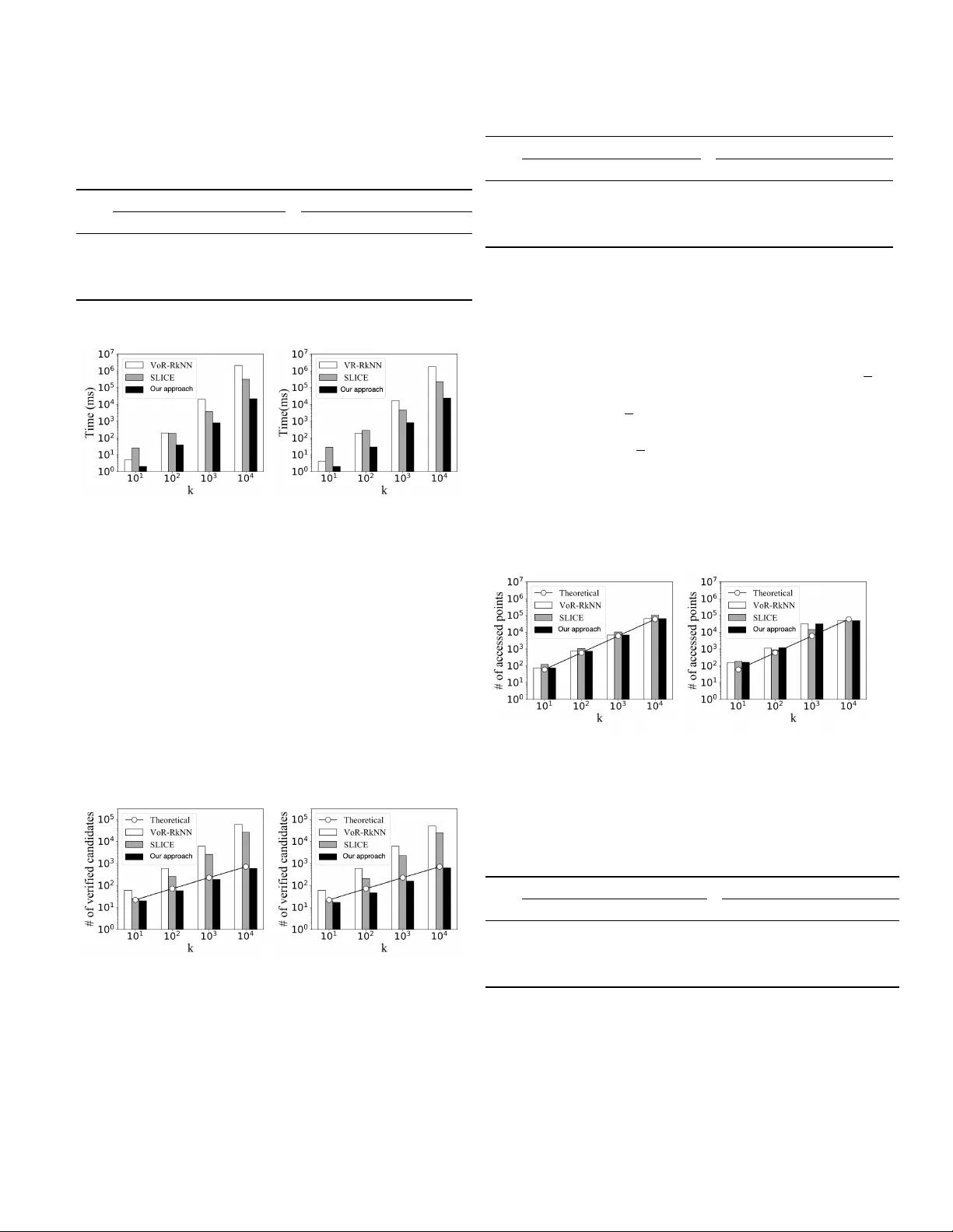
Impro ving Re v erse k Nearest Neighbors Queries Lixin Y e School of Computer Science , China University of Geosciences Abstract —The re verse k nearest neighbor query finds all points that have the query point as one of their k nearest neighbors, where the k NN query finds the k closest points to its query point. Based on conics, we propose an efficent R k NN verification method. By using the proposed verification method, we imple- ment an efficient R k NN algorithm on V oR-tree, which has a computational complexity of O ( k 1 . 5 · log k ) . The comparative experiments are conducted between our algorithm and other two state-of-the-art R k NN algorithms. The experimental r esults indicate that the efficiency of our algorithm is significantly higher than its competitors. Index T erms —R k NN, conic section, V oronoi, Delaunay I . I N T R O D U C T I O N As a v ariant of nearest neighbor (NN) query , RNN query is first introduced by Korn and Muthukrishnan [1]. A direct generalization of NN query is the rev erse k nearest neighbors (R k NN) query , where all points having the query point as one of their k closest points are required to be found. Since its appearance, R k NN has receiv ed extensi ve attention [2], [3], [4], [5], [6], [7] and been prominent in v arious scientific fields including machine learning, decision support, intelligent computation and geographic information systems, etc. At first glance, R k NN and k NN queries appear to be equiv alent, meaning that the results for R k NN and k NN may be the same for the same query point. Howe ver , R k NN is not as simple as it seems to be. It is a very different kind of query from k NN, although their results are similar in many cases. So far , R k NN is still an expensi ve query for its computational complexity at O ( k 2 ) [6], whereas the computational complexity of k NN queries has been reduced to O ( k · log k ) [7]. In order to solve the RNN/R k NN problem, a large number of approaches have been proposed. Some early methods [8], [1], [9] speed up RNN/R k NN queries by pre-computation. Their disadv antage is that it is dif ficult to support queries on dynamic data sets. Therefore, many R k NN algorithms without pre-computation are proposed. Most existing non-pre-computation R k NN algorithms have two phases: the filtering phase and the refining phase (also known as the pruning phase and the verification phase). In the pruning phase, the majority of points that do not belong to R k NN should be filtered out. The main goal of this phase is to generate a candidate set as small as possible. In the verification phase, each candidate point should be verified whether it belongs to the R k NN set or not. For most algorithms, the candidate points are verified by issuing k NN queries or range queries, which are very computational expensi ve. The state- of-the-art R k NN technique SLICE, pro vides a more ef ficient verification method with a computational complexity of O ( k ) for one candidate. The size of the candidate set of SLICE varies form 2 k to 3 . 1 k . Howe ver , it is still time consuming to perform such a verification for each candidate point. There seems to be a consensus in the past studies that for an R k NN technique, the number of verification points cannot be smaller than the size of the result set. Such an idea, howe ver , limits our understanding of the R k NN problem. Hence we amend our thought and come up with a conjecture that whether a point could be directly determined as belonging to the R k NN set according to its location. Gi ven the query point q , our intuition tells us that if a point p is closer to q than a point p + belonging to the R k NNs of q , then p is highly likely to also belong to the R k NN of q . Conv ersely , if p is further away from q than a point p − that does not belong to the R k NN set of q , then p is probably not a member of the R k NN set. Along with this idea, we further study and obtain a set of verification methods for R k NN queries. Based V oR-tree, we use this veirification method implement an efficient R k NN algorithm, which out performs most mainstream algorithms. T ABLE I C O MPA R IS O N O F C O M P U TA T I O NA L C O M P L EX I T Y Operation VR-R k NN SLICE Our approach Generate candidates O ( k · log k ) O ( k · log k ) O ( k · log k ) V erify a candidate O ( k · log k ) O ( k ) O ( k · log k ) | V erified candidates | O ( k ) (=6 k ) O ( k ) (2 k ∼ 3.1 k ) O ( √ k ) ( ≤ 7 . 1 √ k ) Overall O ( k 2 · log k ) O ( k 2 ) O ( k 1 . 5 · log k ) T able I shows the comparison of computational complexity among VR-R k NN , SLICE and our approach. It can be seen that the bottleneck of both VR-R k NN and SLICE is the verification phase. The computational complexity of verifying a candidate of our approach is O ( k · l og k ) , which is higher than that of SLICE. Howe ver , the number of candidates verified by our approach is only about 7 . 1 √ k , which is much less than that of SLICE. In addition, the overall computational complexity of our approach is much lower than that of SLICE. The rest of the paper is organized as follows. In Section 2, we introduce the major related work of R k NN since its appearance. In Section 3, we formally define the R k NN problem and introduce the concepts and knowledge related to our approach. Our approach and its principles are described in section 4. Section 5 provides a detailed theoretical analysis. Experimental ev aluation is demonstrated in Section 6. The last two sections are conclusions and acknowledgements. I I . R E L A T E D W O R K A. RNN-tr ee Rev erse nearest neighbor (RNN) queries are first introduced by K orn and Muthukrishnan where RNN queries are imple- mented by preprocessing the data [1]. For each point p in the database, a circle with p as the center and the distance from p to its nearest neighbor as the radius is pre-calculated and these circles are indexed by an R-tree. The RNN set of a query point q includes all the points whose circle contains q . W ith the R-tree, the RNN set of any query point can be found efficiently . Soon after, sev eral techniques [10], [11] are proposed to impro ve their work. B. Six-r e gions Six-regions [2] algorithm, proposed by Stanoi et al., is the first approach that does not need any pre-computation. They divide the space into six equal segments using six rays starting at the query point, so that the angle between the two boundary rays of each segment is 60 ◦ . They suggest that only the nearest neighbor (NN) of the query point in each of the six segments may belong to the RNN set. It firstly performs six NN queries to find the closest point of the query point q in each segments. Then it launches an NN query for each of the six points to verify q as their NN. Finally the RNN of q is obtained. Generalizing this theory to R k NN queries leads to a corol- lary that, only the members of k NN of the query point in each se gment ha ve the possibility of belonging to the R k NN set. This corollary is widely adopted in the pruning phase of sev eral R k NN techniques. C. TPL TPL [3], proposed by T ao et al., is one of the prestigious algorithms for RkNN queries. This technique prunes the space using the bisectors between the query point and other points. The perpendicular bisector is denoted by B p : q . B p : q is between a point p and the query point q . B p : q divides the space into tw o half-spaces. The half-space that contains p is denoted as H p : q . Another one is denoted as H q : p . If a point p 0 lies in H p : q , p 0 must be closer to p than to q . Then p 0 cannot be the RNN of q and we can say that p prunes p 0 . If a point is pruned by at least k other points, then it cannot belong to the R k NN of q . An area that is the intersection of any combination of k half- spaces can be pruned. The total pruned area corresponds to the union of pruned regions by all such possible combinations of k bisectors (total  m k  combinations). TPL also uses an alternativ e computational cheaper pruning method which has a less pruning power . All the points are sorted by their Hilbert values. Only the combinations of k consecutive points are used to prune the space (total m combinations). D. FINCH FINCH is another famous R k NN algorithm proposed by W u et al. [4]. The authors of FINCH think that it is too computational costly to use m combinations of k bisectors to prune the points. They utilize a con ve x polygon that ap- proximates the unpruned region to prune the points instead of using bisectors. All points lying outside the polygon should be pruned. Since the containment can be achiev ed in logarithmic time for conv ex polygons, the pruning of FINCH has a higher efficienc y than TPL. Ho wev er , the computational complexity of computing the approximately unpruned con ve x polygon is O ( m 3 ) , where m is the number of points considered for pruning. E. InfZone Previous techniques can reduce the candidate set to an extent by different pruning methods. Howe ver , their verifica- tion methods for candidates are very inefficient. It is quite computational costly to issue an inef ficient verification for each point in a candidate set with a size of O( k ). In order to ov ercome this issue, a nov el R k NN technique which is named as InfZone is proposed by Cheema et al. [5]. The authors of InfZone introduce the concept of influence zone (denoted as Z k ), which also can be called R k NN region. The influence zone of a query point q is a region that, a point p belongs to the R k NN set of q , if and only if it lies in the Z k of q . The influence zone is always a star-shaped polygon and the query point is its kernel point. A number of properties are detailed. These properties are aimed to shrink the number of points which are crucial to compute the influence zone. They propose an influence zone computing algorithm with a computational complexity of O ( k · m 2 ) , where m is the number of points accessed during the construction of the influence zone. Every points that lies inside the influence zone are accessed in the pruning phase, since they cannot be ignored during the construction of the influence zone. Namely , all the potential members of the R k NN are accessed during the pruning phase. Hence, for monochromatic R k NN queries, InfZone does not require to verify the candidates. It is indicated that the expected size of R k NN set is k . Evidently , the size of R k NN must not be greater than m , i.e., k ≤ m . Therefore, the computational complexity of InfZone must be no less than O ( k 3 ) . F . SLICE SLICE [6] is the state-of-the-art approach for R k NN queries. In recent years, sev eral well-known techniques [2] hav e been proposed to address the limitations of half-space pruning[3] (e.g., FINCH [4], InfZone [5]). While few re- searcher carries out further research based on the idea of Six- regions. Y ang et al. suggests that the regions-based pruning approach of Six-regions has great potential and proposed an efficient R k NN algorithm SLICE [6]. SLICE uses a more powerful and flexible pruning approach that prunes a much larger area as compared to Six-regions with almost similar computational complexity . Furthermore, it significantly im- prov es the verification phase by computing a list of significant points for each segment. These lists are named as sig List s. Each candidate can be verified by accessing sig List instead of issuing a range query . Therefore, SLICE is significantly more efficient than the other e xisting algorithms. G. VR-R k NN For most R k NN algorithms, data points are inde xed by R- tree [12]. Ho wev er , R-tree is originally designed primarily for range queries. Although some approaches [13], [3], [14], [15] are proposed afterw ards to make it also suitable for NN queries and their variants: the NN derived queries are still disadvantageous. When answering an NN deriv ed query , all nodes in the R-tree intersecting with the local neighborhood (Search Region) of the query point need to be accessed to find all the members of the result set. Once the candidate set of the query is large, the cost of accessing the nodes can also become very large. In order to improve the performance of R- tree on NN deriv ed queries, Sharifzadeh and Shahabi proposes a composite index structure composed of an R-tree and a V oronoi diagram, and named it as V oR-T ree [7]. V oR-T ree benefits from both the neighborhood e xploration capability of V oronoi diagrams and the hierarchical structure of R-tree. By utilizing V oR-tree, they propose VR-R k NN to answer the R k NN query . Similar to the filter phase of Six-regions [2], V or- R k NN di vides the space into 6 equal segments and selects k candidate points from each segment to form a candidate set of size 6 k . During the refining phase, each candidate point is verified to be a member of the R k NN through issuing a k NN query (VR- k NN). The e xpected computational complexity of VR-R k NN is O ( k 2 · l og k ) I I I . P R E L I M I N A R I E S A. Pr oblem definition Definition 1. Euclidean Distance: Gi ven two points A = { a 1 , a 2 , ..., a d } and B = { b 1 , b 2 , ..., b d } in R d , the Euclidean distance between A and B , dist ( A, B ) , is defined as follo ws: dist ( A, B ) = v u u t d X i =1 ( a i − b i ) 2 . (1) Definition 2. k NN Queries: A k NN query is to find the k closest points to the query point from a certain point set. Mathematically , this query in Euclidean space can be stated as follo ws. Giv en a set P of points in R d and a query point q ∈ R d , k NN( q ) = { p ∈ P | dist ( p, q ) ≤ dist ( p k , q ) } where p k is the k th closest point to q in P . (2) Definition 3. R k NN Queries: A R k NN query retriev es all the points that have the query point as one of their k nearest neighbors from a certain point set. Formally , giv en a set P of points in R d and a query point q ∈ P , the R k NN of q in P can be defined as R k NN( q ) = { p ∈ P | q ∈ k NN( p ) } . (3) B. V or onoi diagr am & Delaunay gr aph V oronoi diagram [16], proposed by Rene Descartes in 1644, is a spatial partition structure widely applied in many science domains, especially spatial database and computational geom- etry . In a V oronoi diagram of n points, the space is divided Fig. 1. a) V oronoi Diagram, b) Delaunay Graph into n regions corresponding to these points, which are called V oronoi cells. For each of these n points, the corresponding V oronoi cell consists of all locations closer to that point than to any other . In other words, each point is the nearest neighbor of all the locations in its corresponding V oronoi cell. Formally , the above description can be stated as follows. Definition 4. V oronoi cell & V oronoi diagram: Giv en a set P of n points, the V oronoi cell of a point p ∈ P , denoted as V ( P , p ) or V ( p ) for short, is defined as Equation (4) V ( P , p ) = { q | ∀ p 0 ∈ P \ { p } : dist ( p, q ) ≤ dist ( p 0 , q ) } (4) and the V oronoi diagram of P , denoted as V D ( P ) , is defined as Equation (5). V D ( P ) = { V ( P, p ) | p ∈ P } (5) The V oronoi diagram of a certain set P of points, V D ( P ), is unique. Definition 5. V oronoi neighbor: Given the V oronoi diagram of P , for a point p , its V oronoi neighbors are the points in P whose V oronoi cells share an edge with V ( P, q ) . It is denoted as V N ( P , q ) or V N ( q ) for short. Note that the nearest point in P to p is among V N ( q ) . Lemma 1. Let p k be the k -th nearest neighbor of q , then p k is a V or onoi neighbor of at least one point of the k − 1 near est neighbors of q (where k > 1 ). Pr oof. See [7]. Lemma 2. F or a V or onoi diagram, the expected number of V or onoi neighbors of a gener ator point does not e xceed 6. Pr oof. Let n , n e and n v be the number of generator points, V oronoi edges and V oronoi v ertices of a V oronoi diagram in R 2 , respectiv ely , and assume n ≥ 3 . According to Euler’ s formula, n + n v − n e = 1 (6) Every V oronoi vertex has at least 3 V oronoi edges and each V oronoi edge belongs to two V oronoi vertices. Hence the number of V oronoi edges is not less than 3( n v + 1) / 2 , i.e., n e ≥ 3 2 ( n v + 1) (7) According to Equation (6) and Equation (7), the following relationships holds: n e ≤ 3 n − 6 (8) When the number of generator points is large enough, the av erage number of V oronoi edges per V oronoi cell of a V oronoi diagram in R d is a constant value depending only on d . When d = 2, every V oronoi edge is shared by two V oronoi Cells. Hence the av erage number of V oronoi edges per V oronoi cell does not exceed 6, i.e., 2 · n e /n ≤ 2(3 n − 6) /n = 6 − 12 /n ≤ 6 . For set of points P , a dual graph of its V oronoi Diagram is the Delaunay graph (denoted as D G ( P ) ) [17] of it. For P , its nearest neighbor graph is a subgraph of its Delaunay graph. Definition 6. Delaunay graph distance: Giv en the Delaunay graph D G ( P ) , the Delaunay graph distance between two vertices p and p 0 of D G ( P ) is the minimum number of edges connecting p and p 0 in D G ( P ) . It is denoted as dist DG ( p, p 0 ) . Lemma 3. Given the query point q , if a point p belongs to R k NN( q ), then we have dist DG ( p, q ) ≤ k in Delaunay gr aph D G ( p ) . Pr oof. See [7]. C. Conic section Definition 7. Ellipse: An ellipse is a closed curve on a plane, such that the sum of the distances from any point on the curve to two fix ed points p 1 and p 2 is a constant C . F ormally , it is denoted as E c p 1 : p 2 defined as follo ws: E c p 1 : p 2 = { p | dist ( p, p 1 ) + dist ( p, p 2 ) = C } (9) Definition 8. Hyperbola: A h yperbola is a geometric figure such that the difference between the distances from any point on the figure to two fixed points p 1 and p 2 is a constant C . Formally , it is denoted as H c p 1 : p 2 defined as follo ws: H c p 1 : p 2 = { p | | dist ( p, p 1 ) − dist ( p, p 2 ) | = C } (10) I V . M E T H O D O L O G I E S A. V erification appr oach Fig. 2. k NN region Definition 9. k NN region: Gi ven a query point q , the k NN region of q is the inner region of C q : dist ( q ,p k ) , i.e., the circle with q as center and dist ( q , p k ) as the length of radius, where p k represents the k th closest point to q . This region is denoted as RG k NN ( q ) . The radius of RG k NN ( q ) is called the k NN radius of q and is denoted as r q . Note that a point p must be one k NN( q ) if it lies in RG k NN ( q ) , i.e., the k NN region of q . Con versely , if a point p 0 lies out of RG k NN ( q ) , it cannot be any one of k NN( q ). In Figure 2, q is the query point and the gray re gion within the circle centered on q represents RG k NN ( q ) . As we can see, p 1 , p 2 and p 3 lie inside RG k NN ( q ) , then we can determine that they belong to k NN( q ). while p 4 and p 5 lie outside. So they are not the members of k NN( q ). Lemma 4. Given a query point q , a point p must be one of R k NN( q ) if it satisfies dist ( p, q ) ≤ r p . (11) Con versely , a point p 0 cannot be any one of R k NN( q ) if it satisfies dist ( p 0 , q ) > r p 0 . (12) Simply , for a point p , if the query point q lies in its k NN r e gion, p must be one of R k NN( q ), otherwise it must not belong to R k NN( q ). Pr oof. The lemma is easily prov ed by the definition of k NN and R k NN, see Equation (2) and Equation (3). According to Lemma 4, we can determine whether a point p belongs to the R k NN of the query point q by calculating the k NN region of p . Obviously , q lying in RG k NN ( p ) is a necessary and sufficient condition for p to be one of R k NN( q ). In the refining phase of some R k NN algorithms, the candidates are verified by this condition. In this verification method, k NN re gion is required, so a k NN query must be conducted. The computational complexity of the state-of-the-art k NN algorithm is O ( k · log k ) . Thus, the computational complexity of the verification method based on Lemma 4 is O ( k · l og k ) . For most R k NN algorithms, the size of candidate set is often sev eral times much as that of the result set. Therefore, issuing a R k NN verification of which the computational complexity is O ( k · l og k ) for each candidate is obviously expensi v e. In order to reduce the computational cost of the refining phase of R k NN queries, we introduce sev eral more ef ficient verification approaches in the following. Lemma 5. Given a query point q and a point p + ∈ R k NN( q ), a point p must be one of R k NN( q ) if it satisfies dist ( p, q ) + dist ( p, p + ) ≤ r p + . (13) Pr oof. As sho wn in Figure 3, the larger circle takes p + as the center and r p + as the radius, which represents the k NN region of p + . L p × ,p + is a line segment passing through the point p with a length of r p + . The smaller circle takes p as the center and dist ( p, p × ) as the radius. Let p 0 be an arbitrary point inside C p : dist ( p,p × ) , then it must satisfy that dist ( p, p 0 ) ≤ dist ( p, p × ) . (14) Fig. 3. Lemma 5 According to the triangle inequality , we can obtain dist ( p 0 , p + ) ≤ dist ( p, p 0 ) + dist ( p, p + ) . (15) Combining Inequality (14) and Inequality (15), we can obtain dist ( p 0 , p + ) ≤ dist ( p, p × ) + dist ( p, p + ) = dist ( p × , p + ) = r p + . (16) From abov e, we can construct a corollary that any point lying in C p : dist ( p,p × ) must belong to k NN( p + ). Specifically , the number of points lying in C p : dist ( p,p × ) must not be greater than k , i.e., the size of k NN( p + ). Equiv alently , there is no more than k points closer to p than p × . Thus, p k (the k th closest point to p ) cannot be closer than p × to p . Then dist ( p, p × ) ≤ dist ( p, p k ) = r p . Suppose Inequality (13) holds, dist ( p, q ) ≤ r p + − dist ( p, p + ) = dist ( p × , p + ) − dist ( p, p + ) = dist ( p, p × ) ≤ r p . (17) From Lemma 4 and Inequality (17), we can deduce that p ∈ R k NN( q ). Therefore Lemma 5 prov ed to be true. Lemma 5 provides a sufficient but unnecessary condition for determining that a point belongs to R k NN( q ), where q represents the query point. That means if a point p satisfies the condition of Inequality (13), it can be determined as one of R k NN( q ) without issuing a k NN query . In the case that r p + is known, we can verify whether Inequality (13) holds by only calculating the Euclidean distance from p to q and p + respectiv ely . Calculating the Euclidean distance between two points can be regarded as an atomic operation. Hence the computational complexity of the verification method corresponding to Lemma 5 is O (1) . Definition 10. Positive determine region: Giv en the query point q and a point p , the positiv e determine region of p is the internal region of E r p p : q . Formally , it is denoted as R G + det ( p ) and is defined as follo ws: RG + disc ( p ) = { p 0 | dist ( p 0 , q ) + dist ( p 0 , p ) ≤ r p } . (18) Fig. 4. Positive determine region From the triangle inequality , it can be shown that dist ( p 0 , q ) + dist ( p 0 , p ) ≥ dist ( p, q ) . (19) If p / ∈ R k NN( q ), i.e., dist ( p, q ) > r p , dist ( p 0 , q ) + dist ( p 0 , p ) > r p (20) then R G + det ( p ) = ∅ . Therefore, if RG + det ( p ) 6 = ∅ , p must belong to R k NN( q ). In consequence, from Lemma 5, we can construct a corollary that, for any point p , if R G + det ( p ) is not empty , all the points lying inside of RG + det ( p ) must belong to R k NN( q ). As shown in Figure 4, q represents the query point, the internal region of the circle C p : r p indicates RG k NN ( p ) , and the gray region within the ellipse E r p p : q is for RG + det ( p ) . As p 1 and p 2 lies in RG + det ( p ) , we can know p 1 , p 2 ∈ R k NN( q ). Whereas p 3 , p 4 and p 5 lie out of RG + det ( p ) , so we cannot directly determine whether or not they belong to R k NN( q ) by Lemma 5. Lemma 6. Given a query point q and a point p − / ∈ R k NN( q ), a point p cannot be any one of R k NN( q ) if it satisfies dist ( p, q ) − dist ( p, p − ) > r p − . (21) Fig. 5. Lemma 6 Pr oof. As sho wn in Figure 5, the smaller circle takes p − as the center and r p − as the radius, which represents the k NN region of p − . The point p × is the intersection of an extension of L p,p − (a line segment between p and p − ) with C p − : r p − . The lar ger circle takes p as the center and dist ( p, p × ) as the radius. Let p 0 be an arbitrary point inside of C p − : r p − , then it must satisfy that dist ( p − , p 0 ) ≤ dist ( p − , p × ) = dist ( p − , p × ) . (22) According to the triangle inequality , we can obtain dist ( p, p 0 ) ≤ dist ( p, p − ) + dist ( p − , p 0 ) . (23) From Inequality .(22) and Inequality .(23), we can get that dist ( p, p 0 ) ≤ dist ( p, p − ) + dist ( p − , p × ) = dist ( p, p × ) = r p . (24) Then we realize that all the points lying in RG k NN ( p − ) must lie inside C p : dist ( p,p × ) , namely the number of points lying inside of C p : dist ( p,p × ) must be no less than k , i.e., the number of points lying in R G k NN ( p − ) . That is to say , there exist at least k points no further than p × away from p . Equi v alently , dist ( p, p × ) ≥ dist ( p, p k ) = r p (where p k represents the k th closest point to p ). If the condition of Inequality (21) is satisfied, dist ( p, q ) > dist ( p, p − ) + r p − = dist ( p, p − ) + dist ( p − , p × ) = dist ( p, p × ) ≥ r p . (25) From Lemma 4 and Inequality (25), we can deduce that p / ∈ R k NN( q ). Therefore, Lemma 6 prov ed to be true. From Lemma 6, we can know that, if a point is determined not to be one of R k NN( q ) and its k NN radius is known, then there may exist some other points that can be sufficiently determined to belong to R k NN( q ) without performing a k NN query but by performing two times of simple Euclidean distance calculation. That means the computational complexity of the v erification method based on Lemma 6 is O (1) . Fig. 6. Negativ e determine region Definition 11. Negative determine r egion: Gi ven the query point q and a point p , H r p p : q divides the space into three regions of which the one contains p is the negati ve determine region of p . Formally , this region is denoted as RG − det ( p ) and is defined as follows: RG − det ( p ) = { p 0 | dist ( p 0 , q ) − dist ( p 0 , p ) > r p } . (26) For an arbitrary point p 0 ,from the triangle inequality in 4 pq p 0 , it can be kno wn that dist ( p 0 , p ) + dist ( p, q ) ≥ dist ( p 0 , q ) . (27) If p ∈ R k NN( q ), i.e., dist ( p, q ) ≤ r p , dist ( p 0 , q ) − dist ( p 0 , p ) ≤ dist ( p, q ) ≤ r p (28) then R G − det ( p ) = ∅ . Therefore, if R G − det ( p ) is not empty , p must belong to R k NN( q ). Hence from Lemma 6, we can draw such a corollary that, for an arbitrary point p , if RG − det ( p ) is not empty , any point lying inside RG − det ( p ) cannot belong to R k NN( q ). As shown in Figure 6, q represents the query point, the region within the circle centered on p represents RG k NN ( p ) , and the gray region separated by the hyperbola H r p p : q on the right represents R G − det ( p ) . As in the figure, p 1 and p 2 lie inside RG − det ( p ) , while p 3 and p 4 do not. Then we can determine that p 1 and p 2 must not belong to R k NN( q ), whereas we cannot tell by Lemma 6 whether p 3 or p 4 belongs to R k NN( q ) or not. Definition 12. Positi ve/Negative determine point: Giv en the query point q and two other points p and p 0 , if p 0 lies in RG + det ( p ) , we claim that p is a positive determine point of p 0 and p can positiv e determine p 0 . It is denoted as p + det − − − → p 0 . Similarity , if p 0 lies in RG − det ( p ) , we name that p is a negativ e determine point of p 0 and p can negati ve determine p 0 . It is denoted as p − det − − − → p 0 . If not specified, both of these two types of points may be collecti v ely referred to as determine points and we can use p det − − → p 0 to express that p can dedermine p 0 . Whether a point belongs to the R k NN set of the query point or not, the corresponding v erification method with lo w com- putational complexity is provided. Howe ver , when performing the verification of Lemma 5 or Lemma 6, the distance from the point to be determined to the query point and the posi- tiv e/negati v e determine point should be calculated respecti vely . In order to further improv e the verification efficiency of some points, we propose Lemma 7. Lemma 7. Given a query point q , a point p must be one of R k NN( q ) if it satisfies dist ( p, q ) ≤ r q / 2 . Fig. 7. Lemma 7 Pr oof. In Figure 7, there are three circles, two of which are centered on q and take r q and r q / 2 as the length of their radii, respecti vely . The other circle takes p as the center and dist ( p, q ) as the length of the radius, where p lies in c q : r q / 2 , i.e., dist ( q , p ) ≤ r q / 2 . Let p 0 be an arbitrary point inside of C p : dist ( p,q ) , then it must satisfy that dist ( p, p 0 ) ≤ dist ( q , p ) . (29) From the triangle inequality of 4 pq p 0 , it can be obtained that dist ( q , p 0 ) ≤ dist ( q , p ) + dist ( p, p 0 ) . (30) Then we can get that, dist ( q , p 0 ) ≤ 2 · dist ( q , p ) . (31) Because dist ( q , p ) ≤ r q / 2 , dist ( q , p 0 ) ≤ 2 · r q / 2 = r q (32) That means, any point lying in C p : dist ( p,q ) must belong to k NN( q ). Therefore, the number of points lying in C p : dist ( p,q ) must not be greater than k , i.e., the size of k NN( q ), which means there is no more than k points closer to p than q . Hence p k ( k th closest point to p ) cannot be closer than q to p . Then dist ( p, q ) ≤ dist ( p, p k ) = r p . (33) According to Lemma 4, p ∈ R k NN( q ), then Lemma 7 is prov ed. Fig. 8. Semi- k NN region Definition 13. Semi- k NN region: Given the query point q , the semi- k NN region of q is the internal region of C q : r q / 2 . Formally , it is denoted as S RG k NN ( q ) and is defined as Equation (34). S RG k NN ( q ) = { p | dist ( p, q ) ≤ r q / 2 } (34) As shown in Figure 8, q represents the query point, the region within the larger circle represents RG k NN ( q ) , and the gray region within the smaller circle represents S RG k NN ( q ) . It can be observed from the figure, p 1 and p 2 lie in the gray region, while p 3 , p 4 and p 5 do not. Then p 1 and p 2 can be determined as members of R k NN( q ). Nev ertheless, we cannot determine whether p 3 , p 4 or p 5 belongs to R k NN( q ) or not by Lemma 7 W ith Lemma 4, 5, 6 and 7, we can find all the points in the R k NNs of the query point by verifying only a small portion of points in the candidates. B. Selection of determine points Theoretically , when using Lemma 4, 5, 6 and 7 to verify the candidates, any R k NN point can be considered as a positiv e determine point. Similarly , if a point is not a member of R k NNs, then it can be considered as a negati ve determine point. In other words, all points in the candidate set are eligible to be selected as determine points. Our aim is to issue as few k NN queries as possible in the process of R k NN queries, that is, to use as few determine points as possible to determine all the other points in the candidate set. Therefore, the selection of determine points is very important for impro ving the efficienc y of R k NN queries. Which points should be selected as determine points is what we will scrutinize next. Definition 14. Determine point set: F or a R k NN query , giv en a set S cnd of candidates and denoted as S dist , a determine set is such a set that the following condition is satisfied: ∀ p ∈ S cnd \ S dist , ∃ p 0 ∈ S dist : p 0 det − − → p. (35) Because it is not certain how many points and which points need to be selected as determine points, the total number of schemes for selecting determine points can be as large as | S cnd | P i =1  | S cnd | i  , where | S cnd | means the number of candidates. Hence the computational complexity of finding the absolute optimal one out of all the schemes is as much as O ( k !) . Howe ver , it is not dif ficult to come up with a relatively good determine points selecting scheme, of which the size of the determine set | S dist | is just about O ( √ k ) . For a positive determine point, most of the points in its determine region are closer to the query point than itself. Furthermore, any negati v e determine point is closer to the query point than most of the points in its own determine region. Therefore, a point belonging to R k NNs can rarely be determined by a point closer to the query point than itself, and the probability that a point not belonging to R k NNs can be determined by a point further than itself away from the query point is also very lo w . Therefore, the points which are extremely close to the boundary of the R k NN region (i.e., influence zone [5]) are rarely able to be determined by other points. Thus, these points should be selected as determine points in preference. Ho wev er , it is impossible to directly find these points near the boundary without pre-calculating the R k NN region. Calculating the R k NN region is a very computational costly process for its computational complexity of O ( k 3 ) . While the k NN region of the query point is easy to obtained by issuing a k NN query . Assuming that the points are uniformly distributed, the k NN re gion and the R k NN region of a query point are extremely approximate and the difference between them is negligible. Hence it is a good strategy to preferentially select the points near the boundary of k NN region as the determine points to some extent. As shown in Figure 9, there are some points distributed. The region inside the circle with q as the center represents the k NN region of q . In general, only the points near the boundary of RG k NN ( q ) need to be selected as the determine Fig. 9. Determine point set points and all the other candidate points can be determined by these determine points. In other words, if the points are ev enly distributed, the points near the boundary of RG k NN ( q ) are enough to form a v alid determine set of q . Because the distribution of points is not guaranteed to be absolute uniform, it is not al ways reliable if only the points near the boundary of the kNN region of the query point are taken as determine points for a R k NN query . In order to ensure the reliability of the selection, we propose a strategy to dynamically construct the determine set while verifying the candidate points. First, the candidate points belonging to k NN( q ) are accessed in descending order of distance to q . Then the other candidate points are accessed in ascending order of distance to q . During the process of accessing candidates, once the currently accessed point cannot be determined by any point in the determine point set, this point should be selected as a determine point and put into the determine point set. Otherwise, we can use a corresponding point in the determine point set to determine whether it belongs to R k NNs or not. C. Matching candidate points with determine points Under the above strategy , it is sufficient to ensure that any point not belonging to S dist can be determined by at least one point in S dist . Since the e xpected size of S dist is O ( √ k ) (see Section 5), the computational complexity of finding a determine point for a point by exhaustiv e searching the determine set is O ( √ k ) . Obviously , it is not a good idea to match candidate points with their determine point in this way . Therefore, we propose a method based on V oronoi diagrams to improve the efficiency of this process. Giv en a V oronoi diagram V D ( P ) of a point set P and a continuous region RG , the vast majority of points in R G hav e at least one V oronoi neighbor lying in RG [18]. For any determine point, its determine region is a continuous region (ellipse region or hyperbola region). So for a non-determine point, there is high probability that at least one of its V oronoi neighbors can determine it or shares a determine point with it. Therefore, when accessing a candidate point, if the point can be determined by one of its V oronoi neighbors or the determine point of one of its V oronoi neighbors, this point can be determined whether belongs to the R k NNs. Otherwise, we say that this point is almost impossible to be determined by any known determine point and it should be marked as a determine point. Recall Lemma 2, in two dimensions, the expected number of V oronoi neighbors per point is 6, which is a constant. By using the above approach we can find the determine point for a non-determine point with a computational complexity of O (1) . D. Algorithm In this subsection, we will introduce the implementation of the R k NN algorithm based the abo ve approaches. The pseudocode for the verification methood is shown in Algorithm 1. When verifying a point, we first try to determine whether the point belongs to R k NNs by Lemma 4 (line 2). If this fails, we visit the V oronoi neigbors of the point and try to use Lemma 2 or Lemma3 to determine it (line 10 and line 13). If none of the three lemmas abov e apply to this point, then we issue a k NN query for it and use Lemma 4 to verify it (line 18). Algorithm 1: verify( p, q , k , r q , S v , S det , D det ) Input: the point p to be verified, the query point q , the parameter k , the k NN radius r q of q , the set S v of points that have been visited , the determine point set S det and the dictionary D det that records the corresponding determine points for non-determine points Output: whether p ∈ R k NN ( q ) . 1 S v .add( p ); 2 if dist ( p, q ) ≤ r q / 2 then / * Lemma 7 * / 3 retur n true ; 4 f oreach p n ∈ VN( p ) do 5 if p n ∈ S v then 6 if p n ∈ S det then 7 p det ← − p n ; 8 else 9 p det ← − D det [ p n ] ; 10 if p det ∈ R k NN ( q ) and dist ( p, q ) + dist ( p, p det ) ≤ r p det then / * Lemma 5 * / 11 D det [ p ] ← − p det ; 12 retur n true ; 13 if p det / ∈ R k NN ( q ) and dist ( p, q ) − dist ( p, p det ) > r p det then / * Lemma 6 * / 14 D det [ p ] ← − p det ; 15 retur n false ; 16 r p ← − calculate the k NN radius of p ; 17 S det .add( p ); 18 if r p ≥ dist ( p, q ) then / * Lemma 4 * / 19 retur n true ; 20 else 21 retur n false ; Algorithm 2: R k NN( q ) Input: the query point q Output: R k NN( q 1 S cnd ← − generateCandidates ( q , k ); 2 Sort S cnd in ascending order by the distance to q ; 3 r q ← − calculate the k NN radius of q ; 4 S v ← − ∅ ; 5 S det ← − ∅ ; 6 D det ← − generate an empty dictionary; 7 S R k NN ← − ∅ ; 8 f or i ← − k to 1 do 9 if verify ( S cnd [ i ] , q , k , r q , S v , S det , D det ) then 10 S R k NN .add ( S cnd [ i ]) ; 11 f or i ← − k + 1 to 6 k do 12 if verify ( S cnd [ i ] , q , k , r q , S v , S det , D det ) then 13 S R k NN .add ( S cnd [ i ]) ; 14 retur n S R k NN ; Using the verification approach in Algorithm 1, we imple- ment an efficient R k NN algorithm, as sho wn in Algorithm 2. First we generate the candidate set in the same way as VR- R k NN [7], where the size of candidate is 6 k (line 1). Next, the candidate set is sorted in ascending order by the distance to the query point (line 2). Then the first k elements of the candidate set and the rest of the elements are divided into two groups. The elements in the two groups are verified one by one in the order from back to front and from front to back, respectiv ely (line 8 and line 11). After all candidate points are verified, the R k NNs of the query point is obtained. W e used the same algorithm as VR-R k NN to generate the candidate set, and we do not improve it. The core of this algorithm is still from the Six-regions [2]. In addition, it uses a V oronoi diagram to find the candidate points incrementally according to Lemma 1. By Lemma 3, only the points whose Delaunay distance to the query point is not lar ger than k are eligible to be selected as candidate points. Hence the number of points accessed for finding candidates in the algorithm is guaranteed to be no more than O ( k 2 ) . The pseudocode of the algorithm for generating candidates is presented in Algorithm 3. V . T H E O R E T I C A L A NA L Y S I S In this section, we analyze the expected size of determine point set, the expected number of accessed points and the computational complexity of our algorithm. A. Expected size of determine point set The query point is q , the number of points in R k NN( q ) is | R k NN | , and the number of points near the boundary of RG k NN ( q ) is | S b | . The area and circumference (total length of the boundary) of R G k NN ( q ) are denoted as A R k NN ( q ) and C R k NN ( q ) , respectiv ely . The expected size of the determine point set of q is | S det | . Algorithm 3: pruning( q , k ) Input: the query point q and the parameter k Output: the candidates of R k NN( q ) 1 H ← − M inH eap () ; 2 V isited ← − ∅ ; 3 f or i ← − 1 to 6 do 4 S cnd [ i ] ← − M inH eap () ; 5 f oreach p ∈ VN( q ) do 6 H .push ([1 , p ]) ; 7 V isited.add ( p ) ; 8 while | H | > 0 do 9 [ dist DG ( p ) , p ] ← − H .pop () ; 10 for i ← − 1 to 6 do 11 if S eg ment i contains p then 12 if | S cnd [ i ] | > 0 then 13 p n ← − the last point in S cnd [ i ] ; 14 else 15 p n ← − a point infinitely away from q ; 16 if dist DG ( p ) ≤ k and dist ( q , p ) ≤ dist ( q , p n ) then 17 S cnd [ i ] .push ([ dist ( p, q ) , p ]) ; 18 for each p 0 ∈ VN( p ) do 19 if p 0 / ∈ V isited then 20 dist DG ( p 0 ) ← − dist DG ( p ) + 1 ; 21 H .push ([ dist DG ( p 0 ) , p 0 ]) ; 22 V isited.add ( p 0 ) ; 23 C andidates ← − ∅ ; 24 f or i ← − 1 to 6 do 25 for j ← − 1 to k do 26 C andidates .add( S cnd [ i ] .pop()); 27 retur n C andidates ; It is shown that the expected value of | R k NN | is k [5]. Thus, the radius of the approximate circle of RG k NN ( q ) is equal to r q . Then A R k NN ( q ) = π · r q 2 (36) C R k NN ( q ) = 2 π · r q . (37) The following equation can be obtained from Equation (36) and Equation (37). C R k NN ( q ) = 2 p π · A R k NN ( q ) (38) As the points around the boundary of RG k NN ( q ) consists of two sets of points where one is inside R G k NN ( q ) and the other is outside, | S b | is to | R k NN | what 2 · C R k NN ( q ) is to A R k NN ( q ) , i.e., | S b | = 2 · 2 p π · | R k NN | = 4 √ π · k ≈ 7 . 1 √ k . (39) If all the points near the boundary are selected as the determine points, there must be some redundancy , i.e., the determine region of some points will overlap. Hence the size of the determine point set generated under our strategy is less than the number of the points near the boundary of the R k NN region, i.e, | S det | ≤ 7 . 1 √ k . B. Expected number of accessed points For an R k NN query of q , the candidate points are distributed in an approximately circular region RG cnd ( q ) centered around q , which has an area A cnd ( q ) and a circumference C cnd ( q ) . The expected number of accessed points is | S ac | . In the filtering phase of our approach, the points accessed include all the the candidate points and their V oronoi neighbors. Except for the points in the candidate set, the other accessed points are distributed outside RG cnd ( q ) and adjacent to the boundary of R G cnd ( q ) . Hence | S ac | − | S cnd | is to | S cnd | what C cnd ( q ) is to A cnd ( q ) , i.e., | S ac | − | S cnd | = 2 p π · | S cnd | (40) | S ac | = | S cnd | + 2 p π · | S cnd | = 6 k + 2 √ π · 6 k ≈ 6 k + 8 . 7 √ k (41) Therefore, if the points are distributed uniformly , the expected number of accessed points is approximately 6 k + 8 . 7 √ k . When the points are distributed unevenly , | S ac | becomes larger . Howe v er , it has an upper bound. Recall Lemma 3, we can make deduce that only the points whose Delaunay graph distance to q is not larger than k are eligible to be selected as candidate points. Then | S ac | ≤ k X i =1 2 π · i = ( k 2 + k ) π. (42) C. Computational complexity The expected computational complexity of the filtering phase of our approach is O ( k · log k ) [7]. In the refining phase, we hav e to issue a k NN query with O ( k · l og k ) computational complexity for each determine point, and the size of the determine point set is about 7 . 1 √ k . The other candidates only need to be verified by our ef ficient v erification method. Thus, the computational complexity of the refining phase is O ( k 1 . 5 · log k ) . Hence the overall computational complexity of our R k NN algorithm is O ( k 1 . 5 · l og k ) . V I . E X P E R I M E N T S In the previous section, we discussed the theoretical perfor- mance of our algorithm. In this section, we intend to ev aluate the performance of aspects through comparison experiments. A. Experimental settings In the experiments, we let VR-R k NN [7] and the state-of- the-art R k NN approach SLICE [6] to be the competitors of our method. The settings of our experiment environment are as follows. The experiment is conducted on a personal computer with Python 2.7. The CPU is Intel Core i5-4308U 2.80GHz and the RAM is DDR3 8G. T o be fair , all three methods in the experiment are imple- mented in Python, with six partitions in the pruning phase. W e use two types of experimental data sets: simulated data set and real data set 1 . T o decrease the error of the experiments, we repeat each experiment for 30 times and calculate the average of the results. The query point for each time of the experiment is randomly generated. Our experiments are designed into four sets. The first set of experiments is used to ev aluate the ef fect of the data size on the time cost of the R k NN algorithms. The data size is from 10 3 to 10 6 and the v alue of k is fix ed at 200. The rest of sets are used to ev aluate the effect of the value of k on the time cost, the number of verified points and the number of the accessed points of the R k NN algorithms, respectiv ely . For these three sets of experiments, the size of the simulated data is fixed at 10 6 , the size of the real data is 49,601 and the value of k v aries from 10 1 to 10 4 . B. Experimental r esults T ABLE II T OTA L T I M E CO S T ( IN M S ) OF D I FF E R EN T R k N N A L G O RI T H M S W IT H V A R I OU S SI ZE S OF DAT A S E TS . Algorithm Data size 10 3 10 4 10 5 10 6 VR-R k NN 510 725 728 732 SLICE 232 397 438 441 Our approach 59 65 69 72 Fig. 10. Effect of data size on efficienc y of R k NN queries Figure 10 shows the time cost of the three R k NN algorithms with v arious data sizes. As we can see, when the number of points in the database is significantly much lager than k , the impact of the data size on the time cost of R k NN queries is very limited. If the number of points in the database is small enough to be on the same order of magnitude as k , all points in the database become candidate points. Then the smaller the database size, the less time cost of the R k NN query . When the number of points in the database is abov e 10,000 and the value of k is fix ed at 200, the time cost of our approach is always around 84% and 90% less than that of SLICE and VR-R k NN, 1 49,601 non-duplicative data points on the geographic coordinates of the National Register of Historic Places (http://www .math.uwaterloo.ca/tsp/us/ files/us50000 latlong.txt) respectiv ely . The detailed experimental results are presented in T able II. T ABLE III T OTA L T I M E CO S T ( I N M S ) OF R k N N Q UE R I E S W I T H V A R I OU S V A LU E S O F k . k Simulated data Real data VR-R k NN SLICE Our approach VR-R k NN SLICE Our approach 10 1 5 26 2 4 28 2 10 2 199 193 39 194 283 29 10 3 20576 3759 801 17212 4610 813 10 4 2118391 321233 22077 1829742 226959 23911 (a) Simulated data (b) Real data Fig. 11. Effect of k on efficiency of R k NN queries Figure 11 shows the influence of k on the efficienc y of these three R k NN algorithms, where sub-figure (a) and (b) sho ws the time cost of R k NN queries from simulated data and real data, respectiv ely . As k varies from 10 to 10,000, the time cost of these three algorithms increases. W ith both synthetic data and real data, the query efficiency of our approach is significantly higher than that of the other tw o competitors. W ith the increase of k , this advantage becomes more and more obvious. When k is 10,000, the time cost of our approach is only about 1/10 of that of the state-of-the-art algorithm SLICE. The detailed experimental results are presented in T able III. (a) Simulated data (b) Real data Fig. 12. Effect of k on the number of candidates verified Figure 12 reflects the relationship between k and the number of candidate points verified of the three algorithms in the experiments. Sub-figure (a) and (b) show the experimental results on simulated data and real data, respectiv ely . These two sub-figures also show the theoretical number of candidate T ABLE IV N U MB E R O F C A N D I D A T E S V E R I FIE D B Y R k N N A L G O RI T H M S W IT H V A R I OU S V A L U E S O F k . k Simulated data Real data VR-R k NN SLICE Our approach VR-R k NN SLICE Our approach 10 1 60 25 20 60 20 17 10 2 600 257 57 600 203 46 10 3 6000 2572 186 6000 2257 156 10 4 60000 25675 599 49601 23874 627 points verified with different values of k . During the execution of our algorithm, only the points in the determine point set are verified by issuing k NN queries. Therefore, the number of candidates verified is equal to the size of the determine point set. As we discussed in section V -A, the size of the determine point set is theoretically not larger than 7 . 1 √ k . In consequence, the theoretical number of verified candidates in Figure 12 is 7 . 1 √ k . It can be seen from the figure that the actual number of points verified is slightly less than the theoretical value, 7 . 1 √ k . It indicates that the experimental results are consistent with our analysis. It is also obvious from the figure that the number of verified candidate points of our approach is much smaller than that of the other two algorithms. The detailed e xperimental results are presented in T able IV. (a) Simulated data (b) Real data Fig. 13. Effect of k on the number of points accessed T ABLE V N U MB E R O F AC C E S S ED P O I N T S O F R k NN Q U E R I ES W I T H V AR I O U S V A L U ES O F k . k Simulated data Real data VR-R k NN SLICE Our approach VR-R k NN SLICE Our approach 10 1 76 119 75 153 181 162 10 2 725 1052 728 1108 876 1193 10 3 6721 10211 6731 32031 14359 31717 10 4 63782 102206 63721 49601 49601 49601 Figure 13 shows the number of accessed points of the three algorithms in the experiments and the theoretical number of accessed points of our approach with various values of k , which indirectly reflects their IO cost. It can be seen from sub-figure (a), the number of accessed points of the three algorithms is almost equal in terms of magnitude, and so is the theoretical v alue of our approach. Specifically , the number of accessed points of our approach is slightly smaller than that of SLICE. As shown in sub-figure (b), our approach needs to access more points than SLICE. The reason is that the distribution of real data is very unev en, and our algorithm is more sensitiv e to the distribution of data than SLICE. Note that our approach and VR-R k NN use the same candidate set generation method, so they have almost the same number of accessed points. The detailed experimental results are presented in T able V. From the abov e three experiments, it can be seen that R k NN query efficiency is little affected by the data size, but greatly affected by the value of k . Our approach is significantly more efficient than other algorithms because it requires less verification of candidate points. For data sets with very uneven distribution of points, the candidate set of our approach is relativ ely large, which will affect the IO cost to some extent. Howe v er , the main time cost of the R k NN query is caused by a large number of verification operations rather than IO. Therefore, the distribution of points has little impact on the ov erall performance of our approach. V I I . C O N C L U S I O N S A N D F U T U R E W O R K S In this paper , we propose an efficient approach to verify potential R k NN points without issuing any queries with non- constant computational complexity . W ith the proposed v erifi- cation approach, an ef ficient R k NN algorithm is implemented. The comparative experiments are conducted between the pro- posed R k NN and other two R k NN algorithms of the state- of-the-art. The experimental results show that our algorithm significantly outperforms its competitors in various aspects, except that our algorithm needs to access more points to generate the candidate set when the distribution of points is very uneven. Howe ver , our algorithm does not require costly validation of each candidate point. Hence the distribution of data has v ery limited impact on its ov erall performance. R E F E R E N C E S [1] Flip K orn and S. Muthukrishnan. Influence sets based on rev erse nearest neighbor queries. In Pr oceedings of the 2000 ACM SIGMOD International Conference on Management of Data, May 16-18, 2000, Dallas, T exas, USA , pages 201–212, 2000. [2] Ioana Stanoi, Divyakant Agrawal, and Amr El Abbadi. Reverse nearest neighbor queries for dynamic databases. In 2000 ACM SIGMOD W orkshop on Resear ch Issues in Data Mining and Knowledge Disco very , Dallas, T exas, USA, May 14, 2000 , pages 44–53, 2000. [3] Y ufei T ao, Dimitris Papadias, and Xiang Lian. Reverse knn search in arbitrary dimensionality . In Proceedings of the Thirtieth International Confer ence on V ery Large Data Bases - V olume 30 , VLDB ’04, page 744–755. VLDB Endowment, 2004. [4] W ei W u, Fei Y ang, Chee Y ong Chan, and Kian-Lee T an. FINCH: ev aluating rev erse k-nearest-neighbor queries on location data. PVLDB , 1(1):1056–1067, 2008. [5] Muhammad Aamir Cheema, Xuemin Lin, W enjie Zhang, and Y ing Zhang. Influence zone: Efficiently processing reverse k nearest neighbors queries. In Proceedings of the 27th International Conference on Data Engineering, ICDE 2011, April 11-16, 2011, Hannover , Germany , pages 577–588, 2011. [6] Shiyu Y ang, Muhammad Aamir Cheema, Xuemin Lin, and Y ing Zhang. SLICE: revi ving regions-based pruning for reverse k nearest neighbors queries. In IEEE 30th International Conference on Data Engineering, Chicago, ICDE 2014, IL, USA, Marc h 31 - April 4, 2014 , pages 760– 771, 2014. [7] Mehdi Sharifzadeh and Cyrus Shahabi. V or-tree: R-trees with voronoi diagrams for efficient processing of spatial nearest neighbor queries. Pr oc. VLDB Endow . , 3(1-2):1231–1242, September 2010. [8] Anil Maheshwari, Jan V ahrenhold, and Norbert Zeh. On rev erse nearest neighbor queries. In Proceedings of the 14th Canadian Conference on Computational Geometry , Univer sity of Lethbridge, Alberta, Canada, August 12-14, 2002 , pages 128–132, 2002. [9] Congjun Y ang and King-Ip Lin. An index structure for efficient re verse nearest neighbor queries. In Pr oceedings of the 17th International Confer ence on Data Engineering, April 2-6, 2001, Heidelber g, Germany , pages 485–492, 2001. [10] Congjun Y ang and King-Ip Lin. An index structure for efficient re verse nearest neighbor queries. In Pr oceedings of the 17th International Confer ence on Data Engineering, April 2-6, 2001, Heidelber g, Germany , pages 485–492, 2001. [11] King-Ip Lin, Michael Nolen, and Congjun Y ang. Applying bulk insertion techniques for dynamic reverse nearest neighbor problems. In 7th International Database Engineering and Applications Symposium (IDEAS 2003), 16-18 July 2003, Hong K ong, China , pages 290–297, 2003. [12] Antonin Guttman. R-trees: A dynamic index structure for spatial searching. In Beatrice Y ormark, editor , SIGMOD’84, Pr oceedings of Annual Meeting, Boston, Massachusetts, USA, June 18-21, 1984 , pages 47–57. A CM Press, 1984. [13] G ´ ısli R. Hjaltason and Hanan Samet. Distance browsing in spatial databases. A CM T rans. Database Syst. , 24(2):265–318, 1999. [14] Dimitris Papadias, Y ufei T ao, K yriakos Mouratidis, and Chun Kit Hui. Aggregate nearest neighbor queries in spatial databases. ACM T rans. Database Syst. , 30(2):529–576, 2005. [15] Dimitris Papadias, Y ufei T ao, Greg Fu, and Bernhard Seeger . Progressiv e skyline computation in database systems. A CM T rans. Database Syst. , 30(1):41–82, 2005. [16] Cyrus Shahabi and Mehdi Sharifzadeh. V oronoi diagrams for query processing. In Encyclopedia of GIS. , pages 2446–2452. Springer , 2017. [17] B. Delaunay . Sur la sph ` ere vide. a la m ´ emoire de georges vorono ¨ ı. Bulletin de I’Acad ´ emie des Sciences de I’URSS. Classe des Sciences Math ´ ematiques et Natur elles , 6:793–800, 1934. [18] Y ang Li. Area queries based on voronoi diagrams. CoRR , abs/1912.00426, 2019.